
Introducing Improved Transformer to Land Cover Classification Using Multispectral LiDAR Point Clouds

1
The State Key Laboratory of High-Performance Computing, College of Computer, National University of Defense Technology, Changsha 410073, China
2
Beijing Institute for Advanced Study, National University of Defense Technology, Beijing 100020, China
3
College of Advanced Interdisciplinary Studies, National University of Defense Technology, Changsha 410073, China
4
School of Remote Sensing and Geomatics Engineering, Nanjing University of Information Science and Technology, Nanjing 210044, China
*
Author to whom correspondence should be addressed.
Remote Sens. 2022, 14(15), 3808; https://doi.org/10.3390/rs14153808
Submission received: 21 June 2022
/
Revised: 3 August 2022
/
Accepted: 4 August 2022
/
Published: 7 August 2022
(This article belongs to the Special Issue Advances in Deep Learning Based 3D Scene Understanding from LiDAR)
Abstract
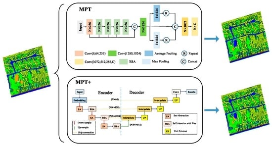
:The use of Transformer-based networks has been proposed for the processing of general point clouds. However, there has been little research related to multispectral LiDAR point clouds that contain both spatial coordinate information and multi-wavelength intensity information. In this paper, we propose networks for multispectral LiDAR point cloud point-by-point classification based on an improved Transformer. Specifically, considering the sparseness of different regions of multispectral LiDAR point clouds, we add a bias to the Transformer to improve its ability to capture local information and construct an easy-to-implement multispectral LiDAR point cloud Transformer (MPT) classification network. The MPT network achieves 78.49% , 94.55% , 84.46% , and 0.92 on the multispectral LiDAR point cloud testing dataset. To further extract the topological relationships between points, we present a standardization set abstraction (SSA) module, which includes the global point information while considering the relationships among the local points. Based on the SSA module, we propose an advanced version called MPT+ for the point-by-point classification of multispectral LiDAR point clouds. The MPT+ network achieves 82.94% , 95.62% , 88.42% , and 0.94 on the same testing dataset. Compared with seven point-based deep learning algorithms, our proposed MPT+ achieves state-of-the-art results for several evaluation metrics.
1. Introduction
Land use and cover change, which are closely related to human development and ecological changes, have long been core areas of global environmental change. A large number of land use research projects have provided knowledge and service support for global and regional land resource surveys [1,2], territorial spatial planning [3], ecological and environmental assessments [4,5], and other governmental decision-making processes and scientific research. Accurate classification is the basis for conducting land cover change research. With the development of industrialization, traditional classification methods based on two-dimensional images can no longer meet the needs of researchers. There is an urgent need for more spatial information to allow for the development of detailed strategies. Therefore, Light Detection and Ranging (LiDAR) data, which can efficiently sense surface and terrain information, are widely used for land cover classification. LiDAR point clouds are a form of data storage.
Compared with two-dimensional images, airborne single-wavelength LiDAR systems can acquire surface information, but they cannot obtain fine classification results. Numerous studies have shown that the performance of single-wavelength LiDAR point clouds can be further improved by combining image information [6,7]. However, determining how to achieve the full fusion of information remains an important issue.
With the development of remote sensing technology, researchers have invented multispectral LiDAR systems that can collect multi-wavelength intensity information simultaneously, provide rich feature information about the target object, and avoid problems associated with data fusion. In 2014, Teledyne Optech developed the first multispectral three-wavelength airborne LiDAR system available for industrial and scientific use. In 2015, Wuhan University developed a four-wavelength LiDAR system. In recent years, multispectral point clouds have been widely used for land cover classification. Wichmann et al. [8] explored the possibility of using multispectral LiDAR point clouds for land cover classification. Bakula et al. [9] further evaluated the performance of multispectral LiDAR point clouds in classification tasks.
Determining how to make full use of multispectral LiDAR point clouds is an important issue. Classical machine learning algorithms are widely used as classifiers for land cover classification [10], for example, through the maximum likelihood method [9,11,12], support vector machine [13,14,15], and random forest [16,17,18] method. With the development of deep learning techniques, convolutional neural network-based algorithms [19,20,21,22,23] have also been successfully applied to multispectral LiDAR point cloud classification. However, due to the disorder of point clouds, the original point clouds need to be transformed into structured data by voxelization or projection. This process inevitably increases the computational burden and leads to a loss of spatial information in some categories, which causes problems of large time consumption and inaccuracy. In 2017, Qi et al. proposed PointNet [24] for the direct processing of conventional point clouds. Inspired by PointNet, researchers have proposed point-based deep learning methods for multispectral LiDAR point clouds. To obtain different channel weights, Jing et al. added the Squeeze-and-Excitation block to PointNet++ [25], and SE-Pointnet++ [26] was developed for the classification of multispectral LiDAR point clouds.
The successful application of Transformer [27] in natural language processing and image processing has attracted researchers to explore its application in 3D point cloud analysis and its ability to achieve state-of-the-art performances in shape classification, part segmentation, semantic segmentation, and normal estimation. Although Transformer-based models can perform well with general point cloud datasets, optimal results are not always achieved with multispectral LiDAR data due to domain gaps [28]. Therefore, we designed Transformer-based networks for multispectral LiDAR point cloud analysis. Our contributions are summarized as follows:
- (1)
- We designed a new Transformer structure to adapt to the sparseness of local regions of the LiDAR point cloud. Specifically, we added a bias to the Transformer, which is named BiasFormer, and changed the normalization methods of the feature maps. Based on BiasFormer, we propose a new multispectral LiDAR point cloud (MPT) classification network, which cascades BiasFormer to capture the deep information in multispectral LiDAR point clouds and uses multilayer perceptrons (MLPs) to accomplish the point-by-point prediction task.
- (2)
- To further capture the topological relationships between points, we propose the SSA module. Specifically, the local contextual information is captured at different scales by iterative farthest point sampling (FPS) and K-nearest neighbor (KNN) algorithms. In each iteration, the point cloud distributions are transformed into normal distributions using the global information from the point clouds and the neighboring information of the centroid points in KNN algorithms to emphasize the influence of neighbor points at different distances to the centroid points. An improved version named MPT+ is proposed for multispectral LiDAR point cloud classification by combining the BiasFormer and SSA modules.
- (3)
- We adopted a weighted cross-entropy loss function to deal with the imbalance among classes and compare the performance of the proposed MPT and MPT+ with seven classical models, thereby confirming the superiority of the proposed networks.
The remainder of this paper is organized as follows: Section 2 introduces the processing methods for general point clouds and the applications of Transformer. Section 3 describes the multispectral LiDAR point clouds and the proposed BiasFormer-based point-by-point classification networks. Section 4 qualitatively and quantitatively analyzes the performance of the MPT and MPT+ networks and compares them with other classical models. Section 5 surveys the effects of different parameters and the weighted cross-entropy loss function on the experimental results. Section 6 concludes the whole paper and presents ideas for further work.
2. Related Work
2.1. Three-Dimensional Point Cloud Processing
Multispectral LiDAR point clouds play an important role in land cover classification. However, the number of multispectral LiDAR datasets is quite small due to the difficulty with data acquisition. Most of the existing methods deal with general point clouds. Given the disorder and irregularity of point clouds, traditional deep-learning-based methods transform point clouds into regularized data by voxelization or projection [29,30,31,32,33,34]. However, the number of voxels generated by the voxel-based network cube increases as the resolution increases, which increases the computational burden. The projection-based networks cause the information inside the point clouds to become folded, which reduces the accuracy. PointNet [24] is a pioneer in the direct processing of 3D point clouds. Subsequently, PointNet++ [25], which captures local point cloud information through a set abstraction module, was proposed. Since then, point-based deep learning networks [20,35,36,37,38], which are dedicated to point cloud analysis, have been influenced by PointNet and PointNet++.
Inspired by PointNet++, researchers were able to deal with local information by grouping. Xiang et al. [37] generated sequences of consecutive point segments to obtain remote point features without expanding the receptive field. Xu et al. [39] proposed a geometric similarity connectivity module to aggregate distant points with similar features and geometric correlations. With this method, the network aggregates neighbor points in Euclidean space and feature space and enhances the robustness of geometric transformations.
Other researchers utilized the graph structures to explore the local features of point clouds. Wang et al. [19] proposed a new neural network module, EdgeConv, to obtain enough local information and extract the global information by stacking EdgeConv modules in DGCNN. Wang et al. [21] proposed a graph attention convolution model that uses attention weights to distinguish different classes of attributes, which allows for the more purposeful learning of matching features. Xu et al. [40] proposed a new sampling approach to construct local graphs and achieved information aggregation on center points.
2.2. Transformer
Bahdanhu et al. [41] applied the attention mechanism to translation work by computing weights through the recurrent neural network. Lin et al. [42] proposed the use of self-attention and used it for the visualization and statement explanation. Based on the self-attention mechanism, Vaswani et al. [27] proposed the Transformer model. Then, researchers [43,44,45,46] further explored the application of Transformers in the field of natural language processing In 2020, Dosovitskiy et al. [47] successfully introduced Transformer to the field of computer vision by proposing Vision Transformer (ViT). Drawing on the success of ViT, researchers have conducted more fruitful work [48,49,50]. Due to the intrinsic structure of Transformer, even a small input can take up a huge amount of storage space. Some useful improvements have been made and are presented in the literature. For example, Lambda attention [51] reconfigures the attention mechanism to achieve linear computation, and SwinTransformer [52] reduces the computational cost by computing over a small window.
Recently, researchers have noticed that the self-attention mechanism of Transformer is essentially a set operator. The successful application of Transformer to 3D point cloud [28,53,54,55,56,57,58,59] analysis suggests that the order invariance is inherently suitable for handling disordered and irregular point clouds. In other words, each point in a point cloud has to perceive information from other points. For example, Point Transformer [53] aggregates the information from K neighbor points to recode points; point cloud Transformer [55] learns features through a self-attention mechanism, and the weight distributions of the proposed model in the paper do not decay with an increasing spatial distance.
3. Dataset and Methods
3.1. Introduction:Dataset
In this study, the experimental dataset was collected by the airborne Titan Multispectral LiDAR system, which contains three wavelengths, the details of which are listed in Table 1.
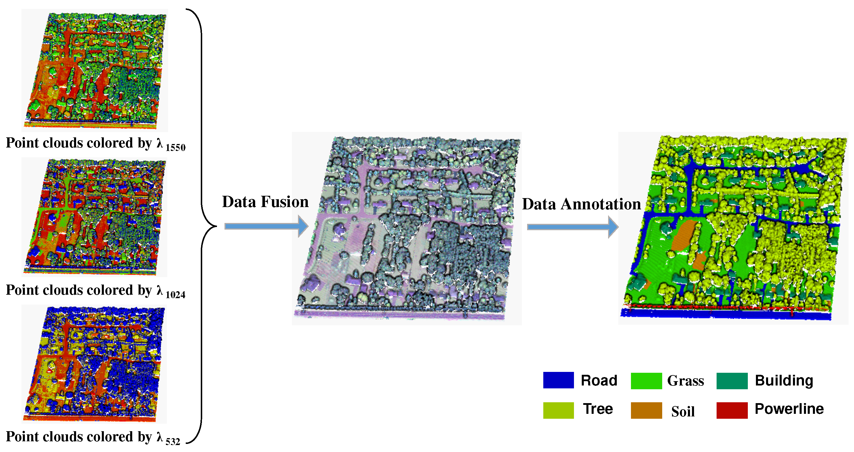
The study area was located in a small town in Ontario, Canada. The longitude and latitude of its central location were 43°58′00″ and 79°15′00″, respectively. The raw data contained the spatial coordinates and intensity values of each wavelength. First, we used the inverse distance-weighted interpolation method to merge the three independent point clouds into one point cloud (Figure 1). The new data contained six dimensions (3D spatial coordinates, and intensity values for the three wavelengths). We divided the area and selected thirteen regions for study. These areas contained six classes, namely roads, buildings, grass, trees, soil, and powerlines. Then, we used CloudCompare software to label the six classes in thirteen regions in a point-by-point manner. We selected the first ten regions for training and the last three regions for testing. The numbers of classes in the training and testing sets are shown in Table 2, where the total numbers in each class in the training and testing sets are presented in bold.
3.2. BiasFormer
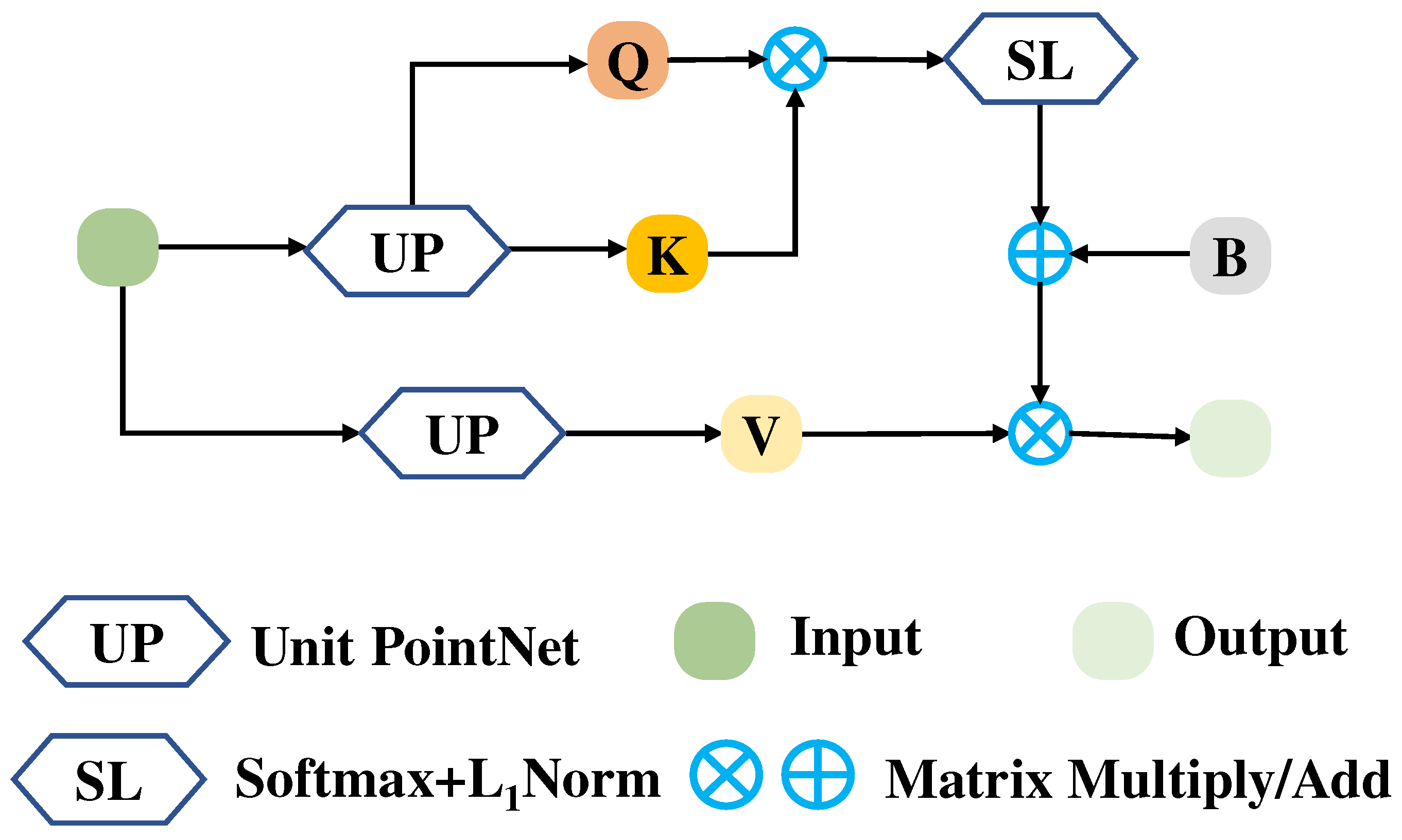
The Transformer maps the input to the query matrix (), key matrix ), and value matrix () through different transformation matrices. The formulas are as follows:
where , and are the learnable weights.
In the original paper [27], the formula for the self-attention operation is as follows:
In this paper, we replace the transformation matrix with the unit PointNet and improve the attention calculation, as follows:
Adding a bias is beneficial to encode the geometric relationship in self-attention calculation. Moreover, we maximize the last dimension and take the norm on the second dimension to highlight the attention weights and reduce the influence of noise [55]. Furthermore, we set to for computational efficiency. Given the LiDAR scan pattern, the sparseness of the multispectral LiDAR point clouds varies greatly among the different regions. The attention mechanism deals with global characteristics but cannot take local characteristics into account. Therefore, we add a learnable bias B after the feature maps to improve the robustness of the model (Figure 2). The improved Transformer is named BiasFormer.
3.3. MPT
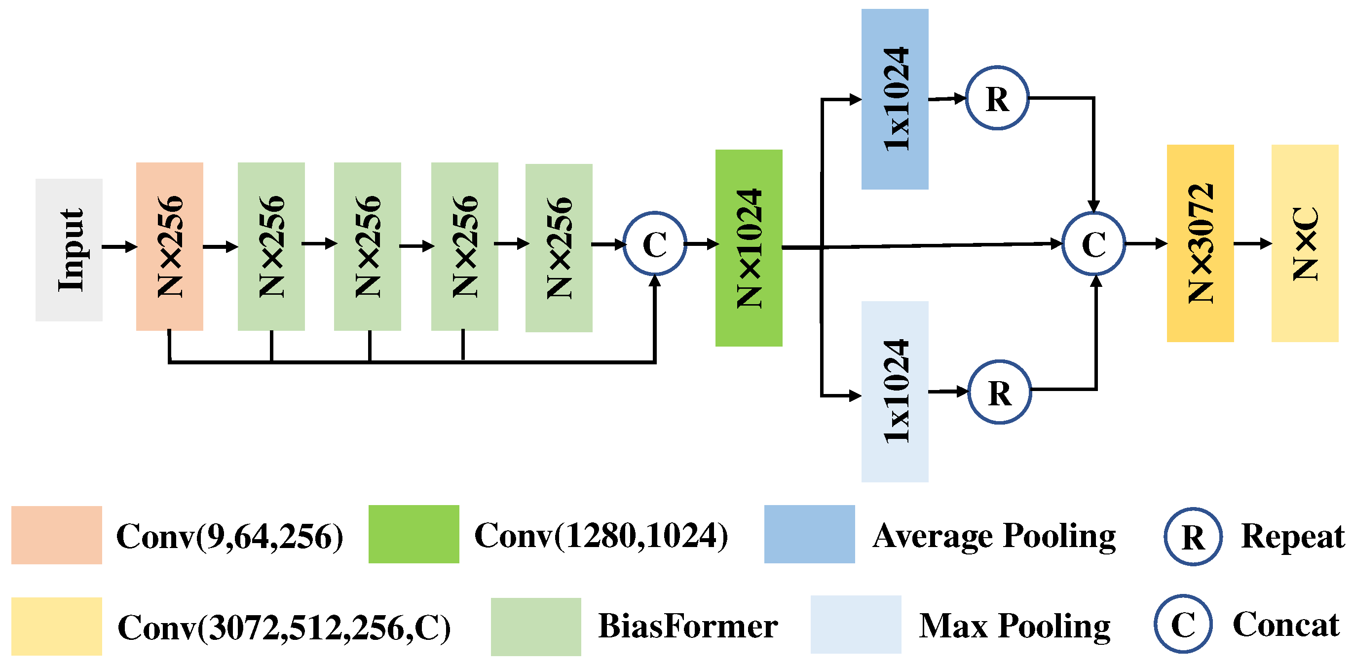
In this section, we propose an end-to-end network (MPT) based on BiasFormer for multispectral LiDAR point cloud classification. We use the same processing method as in PointNet [24] for the S3DIS dataset. N multispectral LiDAR points with 9 attributes (coordinates , 3 wavelength intensities , and normalized coordinates ranging from 0 to 1) are input into the MPT network (Figure 3).
As shown in Figure 3, we map the input to higher dimensions by MLPs to gain richer information. Then, information exchange is carried out through the cascaded four BiasFormers.
represents the i-th BiasFormer, and the dimension of the output feature in each layer is the same as the input. W is the weight of the learnable linear layer.
To include rich point cloud information in global feature vectors, we perform a max pooling operation and an average pooling operation on [19,55]. The obtained features are concatenated with to F to obtain output features, which both contain global information and the individual features of each point cloud. Finally, the probability that each point belongs to six classes is output through the linear layers.
3.4. MPT+
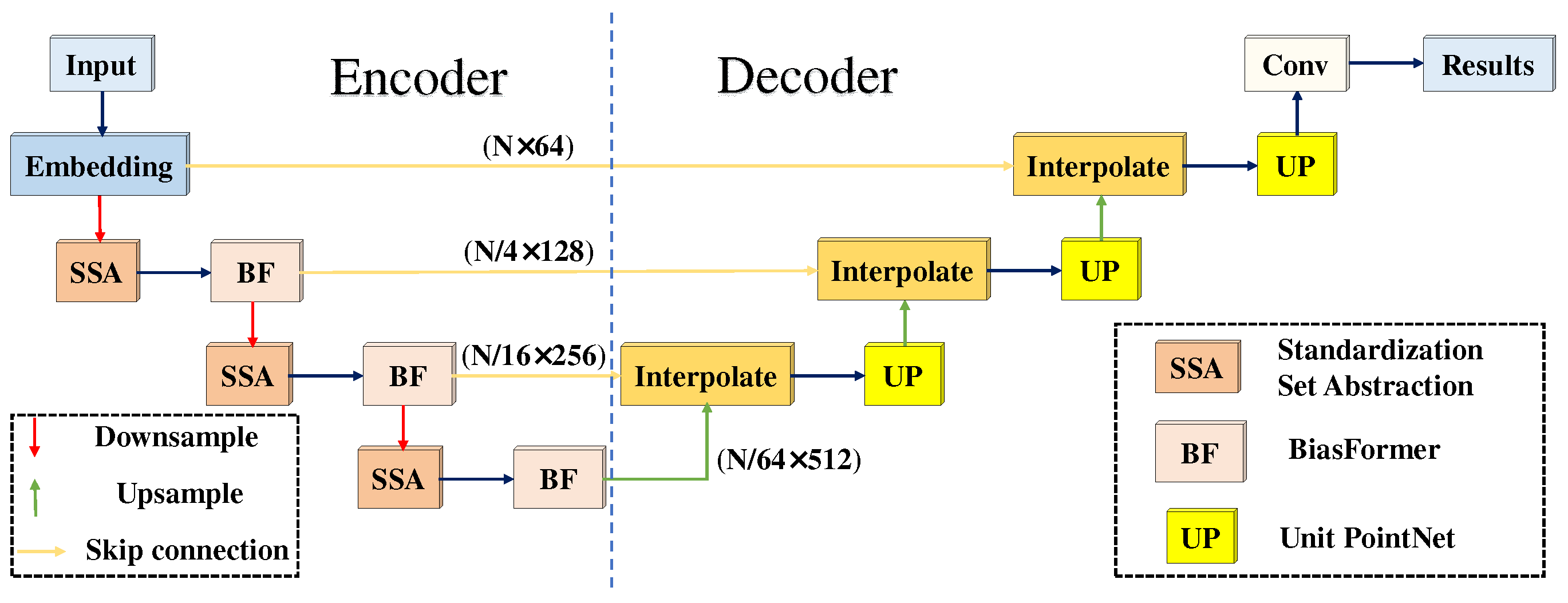
To further determine the relationships among points and extract local features, we propose an advanced version named MPT+ (Figure 4), which recursively feeds multispectral point clouds into the network and expands the context range in a layer-by-layer manner to learn local features. As shown in Figure 4, MPT+ takes a multispectral LiDAR point cloud as the input and outputs the prediction results in a point-by-point manner. MPT+ consists of three parts: an encoding network, a decoding network, and a series of skip connections. The encoding network consists of three cascaded SSAs and BiasFormers. At each level, the input points are first abstracted to generate a new set with fewer elements. Then, the information is exchanged in the global region by BiasFormer. To preserve the low-level abstract information, skip connections mix the features with the same number of point clouds in the encoding network and the decoding network. The decoding network consists of three cascaded feature propagation modules. In each module, the points, the number of which is the same as in the coding layer, are obtained by the interpolation method. Finally, feature fusion is achieved through a unit PointNet. The following subsections detail the point cloud standardization module, the set abstraction module, and the feature propagation module.
3.4.1. Standardization Module
To enhance the robustness of the model, we introduce a standardization module to convert the features at each layer into a normal distribution. Let be the i-th center point, and let be the set of K neighbor points of the i-th center point after KNN sampling. Each neighbor point has d dimensional features. We standardize the local regions using the following formulas:
where and are optimizable parameters, and is the number of center points at the current set abstraction level. We compute the bias by all points of the current set abstraction. Furthermore, we introduce to increase the numerical stability [60]. Through the standardization operation, we change the intensity of the neighbor points without changing the geometric relationship between the neighbor points and the center points.
3.4.2. SSA Module
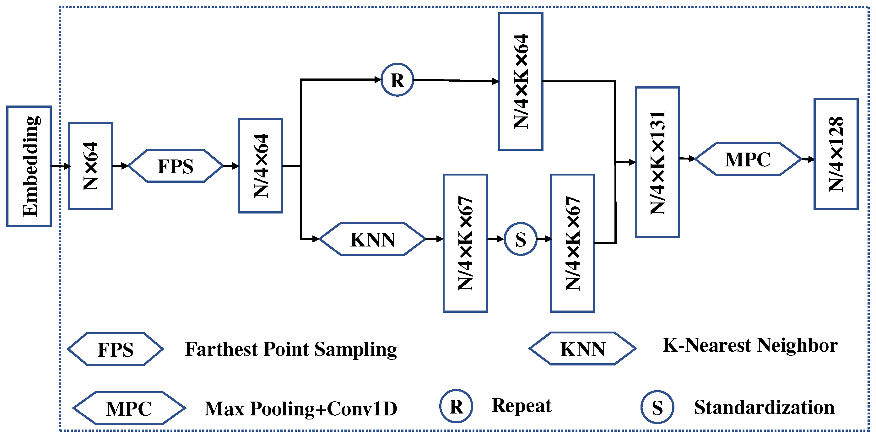
We take the first SSA module as an example to elaborate on the specific operation in the following sections (Figure 5). For a given series of points, , we obtain through the embedding module. We downsample using the FPS method to obtain a subset with a size of , where each point is called a center point. Then, we use the KNN algorithm to extract K closest points to the center point from the initial points and standardize each grouping. After the subset has been obtained using the KNN algorithm, the coordinates of each point in the set are used as information to concatenate the features. At the same time, we copy the subset obtained by downsampling and connect it with the standard set to obtain local region points with a size of . After the max pooling operation and pointwise convolution, the local features are aggregated and interact with each other. The size of the output is .
3.4.3. Feature Propagation Module
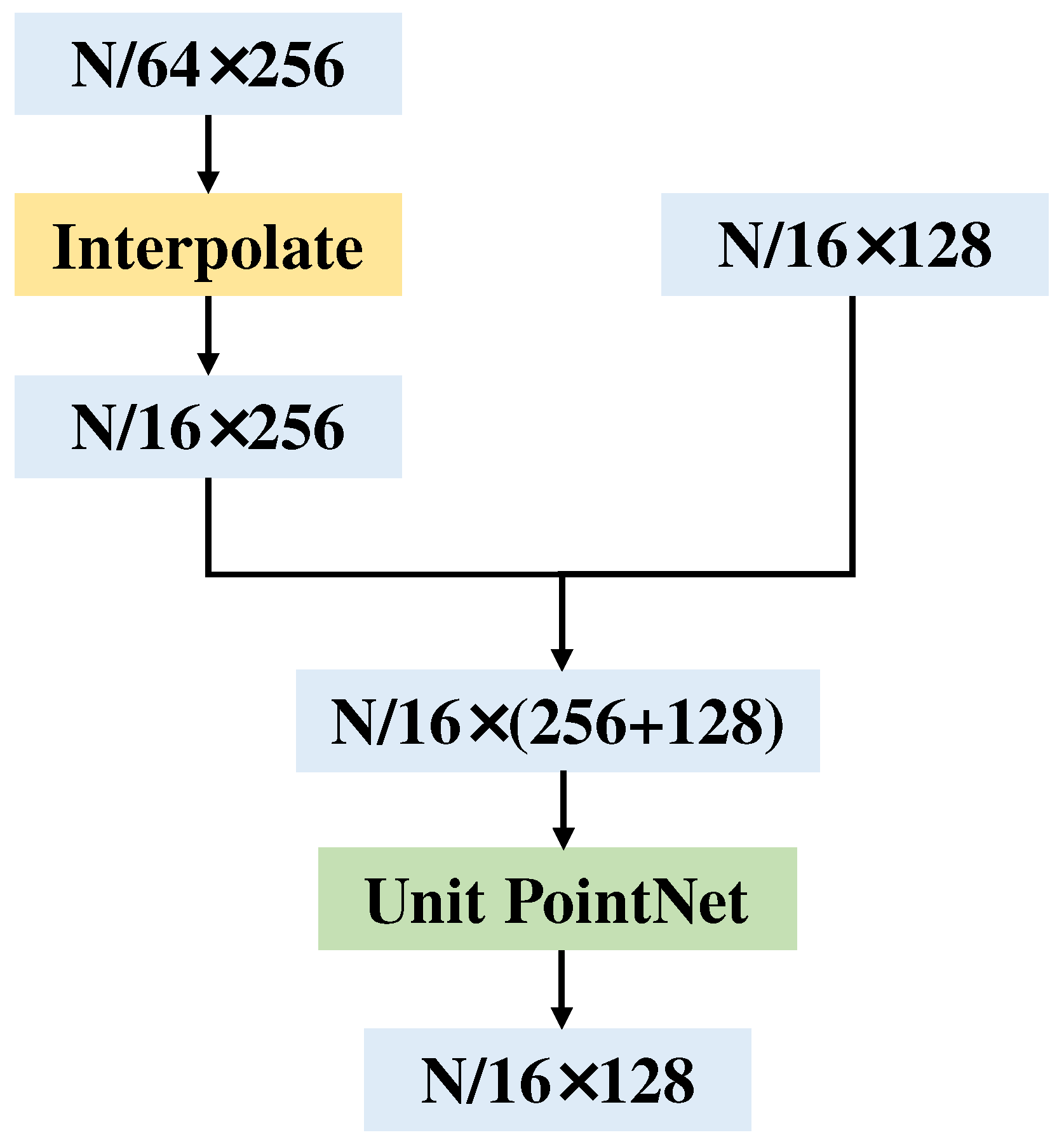
In the SSA module, the multispectral LiDAR point clouds are downsampled several times. However, in the pointwise classification, we need to obtain the features of all original points. We refer to the feature propagation module of PointNet++. In the module, we upsample based on the weights of K nearest neighbors. Taking the first layer of the decoding network as an example, through the interpolation method, points are expanded to and connected with the features in the encoding network. After aggregating the information by the unit PointNet, features with a size of are obtained (Figure 6).
3.5. Loss Function
From Table 2, it can be seen that the class distributions are imbalanced. There are two ways to solve this problem: one is the data-level method, which is achieved by resampling the data with a small sample size; the other is the algorithm-level method, which pays more attention to the small labeled samples in the network. In this study, we used the second method. We adopted the weighted cross-entropy loss function as the loss function of MPT and MPT+ to reduce the impact of class imbalance on the classification results. The following formulas were used:
is the probability that the point belongs to each class, and is the weight of each class. is determined by the total number of samples in the training dataset and the number of samples in class c in the training dataset and is calculated as follows:
where is the number of points in class c, and N is the total number of points in the training dataset. In Section 5.4, comparative experiments show the effectiveness of the weighted cross-entropy loss function.
4. Experiments Settings and Results
In this section, we present the experiments conducted on multispectral LiDAR point clouds to validate and evaluate the performance of the proposed models. First, we elaborate on the software, hardware settings, and metrics used to evaluate the algorithms. Then, we analyze the performance of MPT and MPT+ with the confusion matrix. Finally, we further verify the superiority of the proposed models by comparing them with other popular point-based algorithms.
4.1. Parameter Settings and Evaluation Indicators
All experiments were performed on the Pytorch 1.10.2 platform using an RTX Titan GPU. The key parameter settings of MPT and MPT+ are shown in Table 3.
The following evaluation criteria were used to quantitatively analyze the classification performance of multispectral LiDAR point clouds: the overall accuracy (), Kappa coefficient (), precision (), recall (), (), and Intersection over Union (). Their calculation formulas are as follows:
where represents the number of positive samples predicted by models to be positive, represents the number of negative samples predicted by models to be negative, represents the number of negative samples predicted by models to be positive, represents the number of positive samples predicted by models to be negative, and N represents the total number of labeled samples in the training dataset. Furthermore, according to the elevation information from different classes, we roughly classified the objects into two classes: high elevation and low elevation. High-elevation classes include roads, grass, and soil; whereas low-elevation classes include buildings, trees, and powerlines.
4.2. Performance of MPT and MPT+
In this section, we present the qualitative and quantitative evaluations of the classification performance of the MPT and MPT+ networks on multispectral LiDAR point clouds.
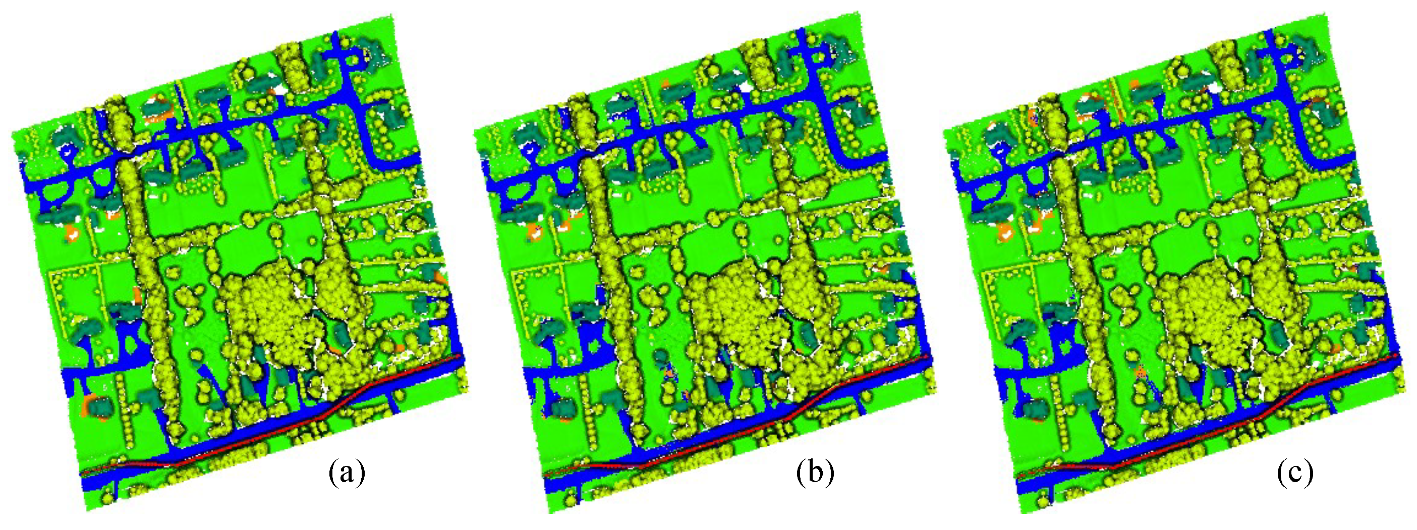
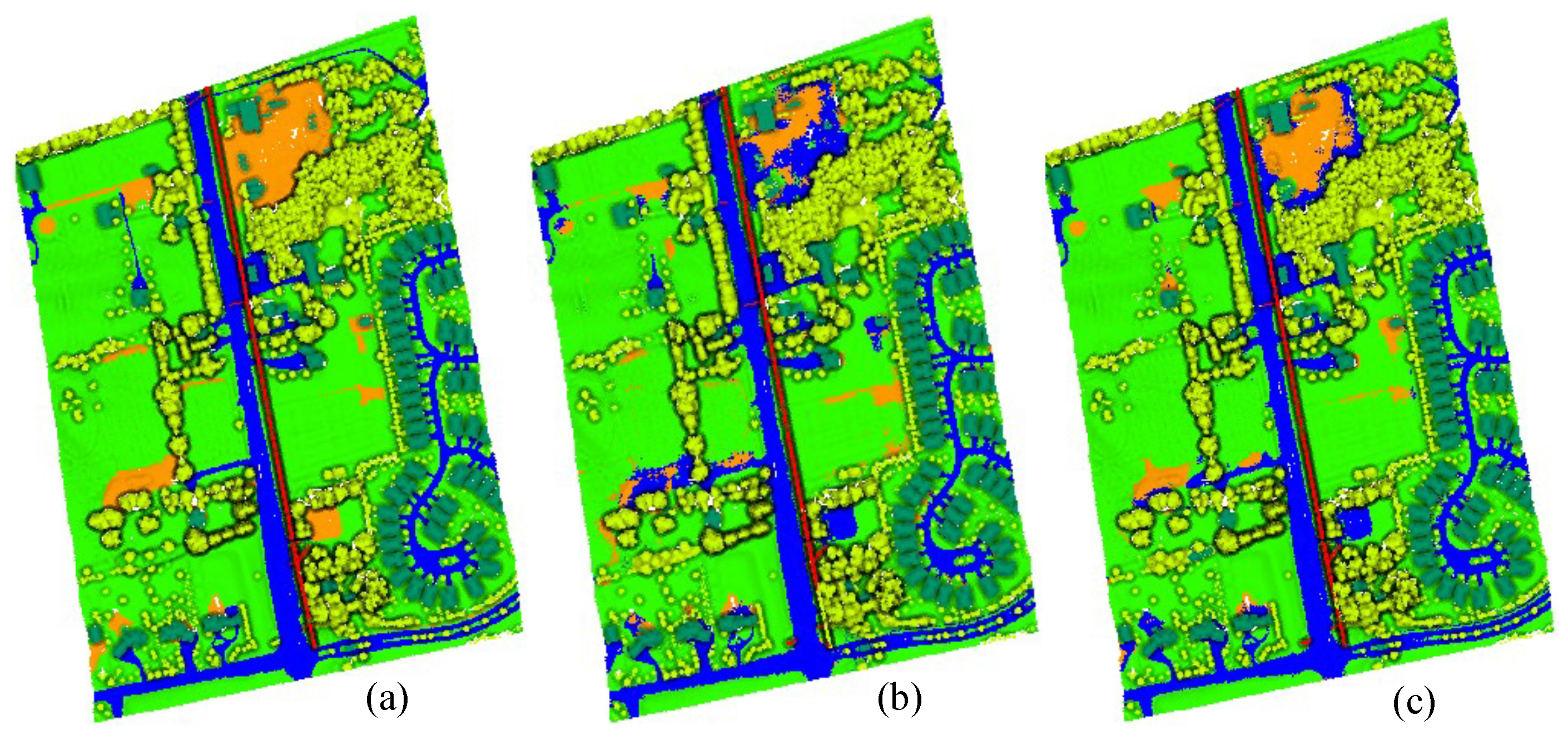
Figure 7, Figure 8 and Figure 9 show the ground truths and prediction results of areas 11–13. As shown in the figures, the classification results for the roads, buildings, grass, trees, and powerlines are satisfactory compared with the ground truths. However, the soil is misclassified as road, which is obvious in Area_11 and Area_13. Furthermore, we can observe that the MPT+ algorithm has fewer misclassified points for soil than the MPT algorithm. However, in small areas, grass, roads, and soil are still easily confused. We speculate that this is because roads, grass, and soil belong to the low-elevation classes. Misclassification points are not easily observed between buildings, trees, and powerlines. Although all three are high-elevation classes, the altitude gaps between the different classes are larger compared to low-elevation classes and are easier to distinguish.
We further quantitatively analyzed the performance of the MPT algorithm and the MPT+ algorithm in Section 4.2.1 and Section 4.2.2 through the confusion matrices of the ground truths and predicted labels.
4.2.1. Results Analysis of the MPT Network
It can be seen from the confusion matrix (Table 4) of the prediction results obtained by the MPT algorithm that roads, buildings, grass, trees, and soil are confused with one another, while the powerlines (strips) only are mistakenly divided into buildings and trees, from which 2705 points are misclassified as buildings and 705 points are misclassified as trees. Additionally, there is more confusion between classes with similar elevations, such as roads, grass, and soil and buildings, trees, and powerlines. It can be seen from the evaluation criteria that trees have the best results with 98.38% , 99.26% , 99.10% , and 99.18% . The soil has the worst results with 20.27% , 44.08% , 27.28% , and 33.70% . In the remaining classes, four evaluation metrics exceed 70%. Furthermore, it is noted that the number of annotated samples for each class in the dataset varies greatly, which has a large impact on the results. Classes with a large number of labeled samples achieve better classification performances, and classes with a small number of labeled samples achieve poor classification performances.
4.2.2. Results Analysis of the MPT+ Network
Table 5 shows the confusion matrix for the prediction results of the MPT+ algorithm. It can be seen from the confusion matrix that the high-elevation classes and the low-elevation classes can be better distinguished. For example, only one road point is mistakenly classified as a building. In classes with similar elevation, the performance of MPT+ is also noteworthy. In the high-elevation classes, MPT+ can fully distinguish buildings from powerlines, and only a small number of buildings (1593 points) are misclassified as trees. Powerlines and trees are also clearly discriminative, with only 88 tree points misclassified as powerlines, and 226 powerline points misclassified as trees. The features of the low-elevation classes are more similar and have more misclassification points. It can be seen from the evaluation indicators that the of roads, grass, and soil reach 78.58%, 93.30%, and 33.03%, respectively. In addition, it can be seen from the classification of each class that the performance of the MPT+ network is better than that of the MPT network. The of roads, buildings, grass, trees, soil, and powerlines increased by 3.78%, 2.21%, 0.76%, 0.67%, 12.76%, and 6.52%, respectively. Among them, the classification results of soil improved most obviously, with 12.76% , 20.65% , 13% , and 15.96% . The classification results confirm the effectiveness of the MPT+ network.
4.3. Comparative Experiments
To the best of our knowledge, there are currently few algorithms that can be applied to multispectral LiDAR point clouds. To demonstrate the effectiveness of our proposed MPT and MPT+ networks, we selected an extensive number of representative point-based deep learning algorithms, including PointNet, PointNet++, DGCNN, GACNet, RSCNN, SE-PointNet++, and PCT. PointNet was the first to attempt to process point clouds directly; Pointnet++, based on PointNet, was proposed to focus on local structures; DGCNN, GACNet, and RSCNN are classic algorithms for processing point clouds; SE-PointNet++ was designed based on the characteristics of spectral LiDAR point clouds; and PCT was one of the earliest algorithms to apply Transformer to point cloud analysis. Table 6 lists the comparison results with the other seven algorithms for the four evaluation indicators.
As can be seen from Table 6, PointNet had the worst performance with 83.79% , 44.28% , 46.68% , and 0.73 . PointNet directly classifies the entire scene point by point, cannot capture the geometric relationships between points, and cannot extract local features. Due to this shortcoming of PointNet, researchers have conducted further investigations. PointNet++ designs a set abstraction module, which captures local context information at different scales by iterating the set abstraction module. DGCNN considers the distances between point coordinates and neighbor points. The relative relationship in the feature space contains semantic features. GACNet establishes the graph structures of each point and neighbor points and calculates the edge weights of the center point and each adjacent point by attention mechanisms so that the network can achieve better results for the edge parts of the segmentation. RSCNN encodes the geometric relationship between points, which expands the application of CNN, and the weights of the CNN are also constrained by the geometric relationship. SE-PointNet++, based on PointNet++, introduces the Squeeze-and-Excitation module to distinguish the influences of different channels on the prediction results. The above algorithms, which do not include PointNet, achieve approximate results (about 90% OA). The Transformer naturally has permutation invariance when dealing with point sequences, making it suitable for disordered point cloud learning tasks. Inspired by Transformer, researchers proposed PCT. It can be seen that, compared with the previous best algorithm, the SE-PointNet++, the , , , and of the PCT network increase by 2.39%, 15.72%, 9.89%, and 0.04, respectively. For the same reason, we improved Transformer. For different point cloud densities in different regions, we added a bias to the Transformer to improve the robustness of the model. The evaluation results of the four indicators show that this method is better than PCT. Based on MPT, we proposed the hierarchical feature extraction network MPT+, which achieved the best results in terms of the four evaluation criteria with 95.62% , 82.94% , 88.42% , and 0.94 .
5. Discussion
From the comparison in Section 4, it is obvious that the performance of the MPT+ network is better than that of the MPT network. Therefore, we performed the parameter analysis only for MPT+. We used the control variable method to analyze the influences of three sensitive parameters (input data, the number of sampling points, the number of neighbor points) on the results. Furthermore, we compared the results with an unweighted loss function. In this section, the values corresponding to each category in the table are the . The for the six categories are calculated for intuitive comparison.
5.1. Impact of Bias
In this section, we verify the effectiveness of adding a bias and the results are shown in Table 7. Adding a bias to the Transformer improved its ability to capture local information. Compared with MPT+, the effect of bias was more obvious in the MPT structure. Moreover, adding a bias was beneficial to encode the geometric relationship in self-attention calculation. Different regions were trained to obtain a bias that was closely related to that region. Among them, the improvement of soil was the most significant. Take soil as an example: the soil distribution was mostly small blocks, and adding a bias was beneficial to obtain better distinction at the boundary.
5.2. Input Data
To demonstrate the role of spectral information in point-by-point classification, we designed five experiments with different types of spectral information input into the proposed MPT+ network. The experiments were as follows: (1) only point cloud coordinates (xyz); (2) point cloud coordinates and 1550 nm wavelength values (xyz + C1); (3) point cloud coordinates and 1064 nm wavelength values (xyz + C2); (4) point cloud coordinates and 532 nm wavelength values (xyz + C3); and (5) point cloud coordinates and three wavelength values (xyz + C123). In the experiment, the number of sampling points was set to 4096, and the number of neighbor points was set to 32.
As can be seen from Table 8, the spectral information improved the performances. The spectrum of each wavelength improved the performance of the point cloud classification compared to inputting only point cloud coordinates. The influences of 1550 nm wavelength values and 532 nm wavelength values on the results were slight and similar, and the influence of the 1064 nm wavelength values on the results was significant. The 1064 nm wavelength values had a greater impact on the five classes, except for soil, and the soil points were more sensitive to the 1550 nm wavelength values. It is worth mentioning that the soil class still had the worst classification results and did not exceed 10% in the four experiments used for comparison, while our input data achieved 33.03% for soil points. Different wavelengths had a superposition effect on the results. Point cloud coordinates and three wavelength values achieved the best results with a 5–9% improvement in and a 2–9% improvement in . Through these comparative experiments, it is confirmed that adding additional spectral information could enhance the accuracy of point-by-point classification and spectral information collected from different channels exhibited different effects on different classes.
5.3. The Number of Sampling Points
The point-by-point classification method required a fixed sample size, therefore, we tested the performance of the model under different training sample sizes. The number of sampling points reflects how local details are captured: the greater the number of sampling points, the richer the captured information and the greater the accuracy. Training samples of different sizes provided different semantic and geometric information on the categories in the scenes. In the experiments, we set N to be 4096, 2048, 1024, and 512, respectively. The other initial parameters remained unchanged. The experimental results are summarized in Table 9.
It can be seen from Table 9 that when the number of sampling points changed from 1024 to 4096, the increased by approximately 3%, doubling the number of sampling points. When the number of sampling points increased from 512 to 1024, the performance improvement was not obvious, and the increased by less than 1%. In addition, OAs became larger with the increase in the number of sampling points. It can be seen that the greater the number of sampling points, the better the classification performance of the multispectral LiDAR point clouds. The experimental results verified our conjecture that a larger sampling size led to better classification accuracy. Considering the limitation of computing power, we need to strike a balance between the accuracy and the number of sampling points. In this paper, we set N to 4096 without further attempts and achieved the best point-by-point classification performance with 82.94% and 95.62% .
5.4. The Number of Neighbor Points
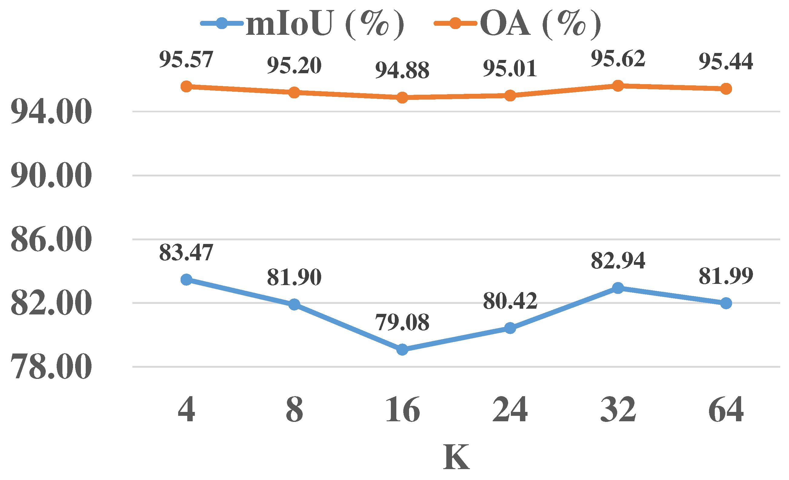
In this section, we explore the effect of the number of neighbor points K on the classification performance. K represents the extent to which the center points obtain the information from surrounding points. The larger the K, the more information is obtained. We set K to 4, 8, 16, 24, 32, and 64 for comparison. The comparison results are shown in Table 10. Other initial parameters remain unchanged.
It can be seen from the table that the prediction results were greatly affected by K, but it was not a simple linear relationship. To visually see that the prediction results are affected by the neighbor points, we plotted the values of and . As can be seen from Figure 10, and did not have a pure polyline relationship. When K was smaller (K = 4 and K = 8), higher and values could be obtained, and when K = 16, both and reached the lowest values. As K increased, and peaked at K = 32. When K = 64, the prediction results started to decrease. We looked at the for each class and found that the soil classification results significantly affected the final results. It can be seen from the ground truths that the soil distribution was concentrated and lumpy. Therefore, when K was small, most of the captured neighbor points were from the soil itself, which allowed better results to be obtained. When K = 16, the captured neighbor point information mixed with other classes, which led to a drop in accuracy. When K was further increased to 32, the model captured more specific local information and geometric relationships between points. When K reached 64, each center point would capture a large number of neighbor points. Due to the sparseness of the different regions of the point clouds, some neighbor points may be farther away and the correlation was insufficient. In addition, noise was also introduced, resulting in decreases in and . Overall, we believe that when K = 32, the model can achieve the best performance.
5.5. Weighted Loss Function
To verify the impact of using the weighted cross-entropy loss function (Case 2) on multispectral point cloud classification, we chose the unweighted cross-entropy loss function (Case 1) for comparison. The experimental results are shown in Table 11. K and N were set as the optimal results obtained in the above comparison (K = 32, N = 4096).
For the class we need to pay attention to, we can give it a higher weight. The higher the weight, the greater the loss, and the better the model will learn this category. If a certain category is less, we can give a higher weight to make it train better. If a certain category does not allow errors, we need to train these data as much as possible, and we can increase its weight. As can be seen from Table 11, the of each class was better when using the weighted cross-entropy loss function than when using the unweighted cross-entropy loss function. Moreover, improved by 1.09% and OA improved by 0.23%. By analyzing the performance of each class, the two classes with the least number of points (soil and powerline) were found to have the most significant improvement, increasing by 4.59% and 0.82% , respectively. We speculate that this is because soil is more easily confused with roads and grass. After the loss function is weighted, it is more sensitive to soil points than road and grass points, so the improvement is greater. The experiments show that the proposed weighted cross-entropy loss function could alleviate the data imbalance problem to a certain extent.
5.6. Computing Resource Analysis
Considering the impact of classification accuracy, we explored the computational resources required by the three best-performing models for point cloud classification. We compared the floating point operations (FLOPs) and parameter quantities of PCT, MPT, and MPT+ (Table 12). It can be seen that, compared with PCT and MPT, MPT+ provides only 14.78 GFLOPs and 1.91M parameters while having a high level of accuracy. MPT+ achieves the best in terms of both computational resource requirements and computational accuracy.
5.7. Experiments on S3DIS Dataset
We test the generalization ability on non-multispectral LiDAR point clouds (S3DIS dataset [61]). The dataset contains 3D scans from Matterport scanners in six areas including 271 rooms. Each point in the scan is annotated with 1 of the semantic labels from 13 categories (chair, table, floor, wall, etc., plus clutter). In contrasting models, the performance of proposed model was only weaker than PointTrans, but achieved the best results in the table and chair classes (Table 13). Our classification accuracy is lower than recently proposed PointTrans by 3.3%, while this small gap validated the good generalization ability of MPT+. Hence, our design could not only deal with a multispectral dataset with complex topology, but also distribute the excellence to regular 3D shapes.
6. Conclusions
In this work, we applied a Transformer to multispectral LiDAR point cloud classification research. Specifically, we proposed BiasFormer, which adds a bias to adapt to the density of different regions of the point cloud and changes the method of normalization.
Based on BiasFormer, we proposed an easy-to-implement multispectral LiDAR point cloud classification network which inputs the encoded point cloud into cascaded BiasFormers and predicts the classes by MLPs. To further differentiate the influences of local regions, we built an SSA module and proposed an improved Multispectral LiDAR point cloud classification (MPT+) network. The MPT+ network gradually expands the receptive field through recursive sampling to allow a wider range of information to be perceived. Qualitative and quantitative analyses were used to demonstrate the feasibility of the use of the MPT and MPT+ networks for carrying out multispectral LiDAR point cloud classification. In addition, we explored the influences of the spectra of different wavelengths, the number of neighbor points, and the number of sampling points on the performance of the control variable method; we obtained the best classification results based on optimal parameters. Furthermore, to deal with the class imbalance problem, we adopted a weighted cross-entropy loss function and improved the IoU by 4.59% on soil points. Finally, we compared the computational resources of the three best-performing networks and verified the superiority of our proposed models in terms of computational resource requirements and performance.
However, there is still a lot of room for improvement in soil points. In future work, we will explore the handling of sample imbalance, enhance the robustness and uniqueness of output features, and improve the accuracy of multispectral LiDAR point cloud classification.
Author Contributions
Methodology, Z.Z.; validation, Z.Z. and T.L.; writing—original draft preparation, Z.Z. and X.T.; writing—review and editing, Z.Z. and X.L.; resources, Z.Z. and Y.P. All authors have read and agreed to the published version of the manuscript.
Funding
This research was partially supported by the National Natural Science Foundation of China (grant numbers 91948303-1 and 61803375) and the Postgraduate Scientific Research Innovation Project of Hunan Province (grant number QL20210018).
Data Availability Statement
No new data were created or analyzed in this study. Data sharing is not applicable to this article.
Acknowledgments
The authors acknowledge the State Key Laboratory of High-Performance Computing, College of Computer, National University of Defense Technology, China. The authors would also like to thank Jonathan Li.
Conflicts of Interest
The authors declare no conflict of interest.
Abbreviations
The following abbreviations are used in this manuscript:
| SSA | standardization set abstraction |
| FPS | farthest point sampling |
| KNN | K-nearest neighbor |
| ViT | vision Transformer |
| overall accuracy | |
| DGCNN | dynamic graph convolution neural network |
| GACNet | graph attention convolution network |
| RSCNN | relation-shape convolution neural network |
| PCT | point cloud transformer |
| FLOPs | floating point operations |
References
- Pocewicz, A.; Nielsen-Pincus, M.; Goldberg, C.S.; Johnson, M.H.; Morgan, P.; Force, J.E.; Waits, L.P.; Vierling, L. Predicting land use change: Comparison of models based on landowner surveys and historical land cover trends. Landsc. Ecol. 2008, 23, 195–210. [Google Scholar] [CrossRef]
- MacAlister, C.; Mahaxay, M. Mapping wetlands in the Lower Mekong Basin for wetland resource and conservation management using Landsat ETM images and field survey data. J. Environ. Manag. 2009, 90, 2130–2137. [Google Scholar] [CrossRef] [PubMed]
- Zhao, J.; Zhao, X.; Liang, S.; Zhou, T.; Du, X.; Xu, P.; Wu, D. Assessing the thermal contributions of urban land cover types. Landsc. Urban Plan. 2020, 204, 103927. [Google Scholar] [CrossRef]
- Scaioni, M.; Höfle, B.; Kersting, A.B.; Barazzetti, L.; Previtali, M.; Wujanz, D. Methods from information extraction from lidar intensity data and multispectral lidar technology. ISPRS J. Photogramm. Remote Sens. 2018, 42, 1503–1510. [Google Scholar] [CrossRef] [Green Version]
- Li, W.; Wang, F.D.; Xia, G.S. A geometry-attentional network for ALS point cloud classification. ISPRS J. Photogramm. Remote Sens. 2020, 164, 26–40. [Google Scholar] [CrossRef]
- Kim, Y.; Kim, Y. Improved classification accuracy based on the output-level fusion of high-resolution satellite images and airborne LiDAR data in urban area. IEEE Geosci. Remote Sens. Lett. 2013, 11, 636–640. [Google Scholar]
- Hong, D.; Gao, L.; Yokoya, N.; Yao, J.; Chanussot, J.; Du, Q.; Zhang, B. More diverse means better: Multimodal deep learning meets remote-sensing imagery classification. IEEE Trans. Geosci. Remote Sens. 2020, 59, 4340–4354. [Google Scholar] [CrossRef]
- Wichmann, V. Evaluating the Potential of Multispectral Airborne LiDAR For Topographic Mapping and Land Cover Classification. ISPRS Ann. Photogramm. Remote Sens. Spat. Inf. Sci. 2015, 2, 113–119. [Google Scholar] [CrossRef] [Green Version]
- Bakuła, K.; Kupidura, P.; Jełowicki, Ł. Testing of Land Cover Classification from Multispectral Airborne Laser Scanning Data. Int. Arch. Photogramm. Remote Sens. Spat. Inf. Sci. 2016, 41, 161–169. [Google Scholar] [CrossRef] [Green Version]
- Liu, X.; Wang, L.; Zhang, J.; Yin, J.; Liu, H. Global and Local Structure Preservation for Feature Selection. IEEE Trans. Neural Netw. Learn. Syst. 2017, 25, 1083–1095. [Google Scholar]
- Morsy, S.; Shaker, A.; El-Rabbany, A. Clustering of Multispectral Airborne Laser Scanning Data Using Gaussian Decomposition. Int. Arch. Photogramm. Remote Sens. Spat. Inf. Sci. 2017, 42, 269–276. [Google Scholar] [CrossRef] [Green Version]
- Fernandez-Diaz, J.C.; Carter, W.E.; Glennie, C.; Shrestha, R.L.; Pan, Z.; Ekhtari, N.; Singhania, A.; Hauser, D.; Sartori, M. Capability assessment and performance metrics for the Titan multispectral mapping lidar. Remote Sens. 2016, 8, 936. [Google Scholar] [CrossRef] [Green Version]
- Teo, T.A.; Wu, H.M. Analysis of land cover classification using multi-wavelength LiDAR system. Appl. Sci. 2017, 7, 663. [Google Scholar] [CrossRef] [Green Version]
- Ekhtari, N.; Glennie, C.; Fernandez-Diaz, J.C. Classification of airborne multispectral lidar point clouds for land cover mapping. IEEE J. Sel. Top. Appl. Earth Obs. Remote Sens. 2018, 11, 2068–2078. [Google Scholar] [CrossRef]
- Xie, Z.; Kai, X.; Liu, L.; Xiong, Y. 3D Shape Segmentation and Labeling via Extreme Learning Machine. Comput. Graph. Forum 2015, 33, 85–95. [Google Scholar] [CrossRef]
- Karila, K.; Matikainen, L.; Puttonen, E.; Hyyppä, J. Feasibility of multispectral airborne laser scanning data for road mapping. IEEE Geosci. Remote Sens. Lett. 2017, 14, 294–298. [Google Scholar] [CrossRef]
- Matikainen, L.; Karila, K.; Hyyppä, J.; Litkey, P.; Puttonen, E.; Ahokas, E. Object-based analysis of multispectral airborne laser scanner data for land cover classification and map updating. ISPRS J. Photogramm. Remote Sens. 2017, 128, 298–313. [Google Scholar] [CrossRef]
- Matikainen, L.; Hyyppä, J.; Litkey, P. Multispectral Airborne Laser Scanning for Automated Map Updating. Int. Arch. Photogramm. Remote Sens. Spat. Inf. Sci. 2016, 41, 323–330. [Google Scholar] [CrossRef] [Green Version]
- Wang, Y.; Sun, Y.; Liu, Z.; Sarma, S.E.; Bronstein, M.M.; Solomon, J.M. Dynamic graph cnn for learning on point clouds. ACM Trans. Graph. Tog 2019, 38, 1–12. [Google Scholar] [CrossRef] [Green Version]
- Liu, Y.; Fan, B.; Xiang, S.; Pan, C. Relation-shape convolutional neural network for point cloud analysis. In Proceedings of the IEEE/CVF Conference on Computer Vision and Pattern Recognition, Long Beach, CA, USA, 15–20 June 2019; pp. 8895–8904. [Google Scholar]
- Wang, L.; Huang, Y.; Hou, Y.; Zhang, S.; Shan, J. Graph attention convolution for point cloud semantic segmentation. In Proceedings of the IEEE/CVF Conference on Computer Vision and Pattern Recognition, Long Beach, CA, USA, 15–20 June 2019; pp. 10296–10305. [Google Scholar]
- Sarode, V.; Dhagat, A.; Srivatsan, R.A.; Zevallos, N.; Lucey, S.; Choset, H. MaskNet: A fully-convolutional network to estimate inlier points. In Proceedings of the 2020 International Conference on 3D Vision (3DV), Fukuoka, Japan, 25–28 November 2020; pp. 1029–1038. [Google Scholar]
- Wen, C.; Li, X.; Yao, X.; Peng, L.; Chi, T. Airborne lidar point cloud classification with graph attention convolution neural network. arXiv 2020, arXiv:2004.09057. [Google Scholar] [CrossRef]
- Qi, C.R.; Su, H.; Mo, K.; Guibas, L.J. Pointnet: Deep learning on point sets for 3d classification and segmentation. In Proceedings of the IEEE Conference on Computer Vision and Pattern Recognition, Honolulu, HI, USA, 21–26 July 2017; pp. 652–660. [Google Scholar]
- Qi, C.R.; Yi, L.; Su, H.; Guibas, L.J. Pointnet++: Deep hierarchical feature learning on point sets in a metric space. Adv. Neural Inf. Process. Syst. 2017, 30, 4–7. [Google Scholar]
- Jing, Z.; Guan, H.; Zhao, P.; Li, D.; Yu, Y.; Zang, Y.; Wang, H.; Li, J. Multispectral LiDAR point cloud classification using SE-PointNet++. Remote Sens. 2021, 13, 2516. [Google Scholar] [CrossRef]
- Vaswani, A.; Shazeer, N.; Parmar, N.; Uszkoreit, J.; Jones, L.; Gomez, A.N.; Kaiser, Ł.; Polosukhin, I. Attention is all you need. Adv. Neural Inf. Process. Syst. 2017, 30, 5998–6008. [Google Scholar]
- Yu, J.; Zhang, C.; Wang, H.; Zhang, D.; Song, Y.; Xiang, T.; Liu, D.; Cai, W. 3d medical point transformer: Introducing convolution to attention networks for medical point cloud analysis. arXiv 2021, arXiv:2112.04863. [Google Scholar]
- Wu, Z.; Song, S.; Khosla, A.; Yu, F.; Zhang, L.; Tang, X.; Xiao, J. 3d shapenets: A deep representation for volumetric shapes. In Proceedings of the IEEE Conference on Computer Vision and Pattern Recognition, Boston, MA, USA, 7–12 June 2015; pp. 1912–1920. [Google Scholar]
- Qi, C.R.; Su, H.; Nießner, M.; Dai, A.; Yan, M.; Guibas, L.J. Volumetric and multi-view cnns for object classification on 3d data. In Proceedings of the IEEE Conference on Computer Vision and Pattern Recognition, Las Vegas, NV, USA, 27–30 June 2016; pp. 5648–5656. [Google Scholar]
- Maturana, D.; Scherer, S. Voxnet: A 3d convolutional neural network for real-time object recognition. In Proceedings of the 2015 IEEE/RSJ International Conference on Intelligent Robots and Systems (IROS), Hamburg, Germany, 28 September–2 October 2015; pp. 922–928. [Google Scholar]
- Xie, J.; Dai, G.; Zhu, F.; Wong, E.K.; Fang, Y. Deepshape: Deep-learned shape descriptor for 3d shape retrieval. IEEE Trans. Pattern Anal. Mach. Intell. 2016, 39, 1335–1345. [Google Scholar] [CrossRef]
- Wu, J.; Zhang, C.; Xue, T.; Freeman, B.; Tenenbaum, J. Learning a probabilistic latent space of object shapes via 3d generative-adversarial modeling. arXiv 2016, arXiv:1610.07584. [Google Scholar]
- Su, H.; Maji, S.; Kalogerakis, E.; Learned-Miller, E. Multi-view convolutional neural networks for 3d shape recognition. In Proceedings of the IEEE International Conference on Computer Vision, Santiago, Chile, 7–13 December 2015; pp. 945–953. [Google Scholar]
- Shi, W.; Rajkumar, R. Point-gnn: Graph neural network for 3d object detection in a point cloud. In Proceedings of the IEEE/CVF Conference on Computer Vision And Pattern Recognition, Seattle, WA, USA, 13–19 June 2020; pp. 1711–1719. [Google Scholar]
- Li, Y.; Bu, R.; Sun, M.; Wu, W.; Di, X.; Chen, B. Pointcnn: Convolution on x-transformed points. arXiv 2018, arXiv:07791.2018. [Google Scholar]
- Xiang, T.; Zhang, C.; Song, Y.; Yu, J.; Cai, W. Walk in the cloud: Learning curves for point clouds shape analysis. In Proceedings of the IEEE/CVF International Conference on Computer Vision, Montreal, QC, Canada, 10–17 October 2021; pp. 915–924. [Google Scholar]
- Zhang, C.; Yu, J.; Song, Y.; Cai, W. Exploiting edge-oriented reasoning for 3d point-based scene graph analysis. In Proceedings of the IEEE/CVF Conference on Computer Vision and Pattern Recognition, Nashville, TN, USA, 20–25 June 2021; pp. 9705–9715. [Google Scholar]
- Xu, M.; Zhou, Z.; Qiao, Y. Geometry sharing network for 3d point cloud classification and segmentation. In Proceedings of the AAAI Conference on Artificial Intelligence, New York, NY, USA, 7–12 February 2020; Volume 34, pp. 12500–12507. [Google Scholar]
- Xu, Q.; Sun, X.; Wu, C.Y.; Wang, P.; Neumann, U. Grid-gcn for fast and scalable point cloud learning. In Proceedings of the IEEE/CVF Conference on Computer Vision and Pattern Recognition, Seattle, WA, USA, 13–19 June 2020; pp. 5661–5670. [Google Scholar]
- Bahdanau, D.; Cho, K.; Bengio, Y. Neural machine translation by jointly learning to align and translate. arXiv 2014, arXiv:1409.0473. [Google Scholar]
- Lin, Z.; Feng, M.; dos Santos, C.N.; Yu, M.; Xiang, B.; Zhou, B.; Bengio, Y. A structured self-attentive sentence embedding. arXiv 2017, arXiv:1703.03130. [Google Scholar]
- Devlin, J.; Chang, M.W.; Lee, K.; Toutanova, K. Bert: Pre-training of deep bidirectional transformers for language understanding. arXiv 2018, arXiv:1810.04805. [Google Scholar]
- Yang, Z.; Dai, Z.; Yang, Y.; Carbonell, J.; Salakhutdinov, R.R.; Le, Q.V. Xlnet: Generalized autoregressive pretraining for language understanding. arXiv 2019, arXiv:1906.08237. [Google Scholar]
- Dai, Z.; Yang, Z.; Yang, Y.; Carbonell, J.; Le, Q.V.; Salakhutdinov, R. Transformer-xl: Attentive language models beyond a fixed-length context. arXiv 2019, arXiv:1901.02860. [Google Scholar]
- Lee, J.; Yoon, W.; Kim, S.; Kim, D.; Kim, S.; So, C.H.; Kang, J. BioBERT: A pre-trained biomedical language representation model for biomedical text mining. Bioinformatics 2020, 36, 1234–1240. [Google Scholar] [CrossRef] [PubMed]
- Dosovitskiy, A.; Beyer, L.; Kolesnikov, A.; Weissenborn, D.; Zhai, X.; Unterthiner, T.; Dehghani, M.; Minderer, M.; Heigold, G.; Gelly, S.; et al. An image is worth 16x16 words: Transformers for image recognition at scale. arXiv 2020, arXiv:2010.11929. [Google Scholar]
- Wu, Z.; Liu, Z.; Lin, J.; Lin, Y.; Han, S. Lite transformer with long-short range attention. arXiv 2020, arXiv:2004.11886. [Google Scholar]
- Wu, H.; Xiao, B.; Codella, N.; Liu, M.; Dai, X.; Yuan, L.; Zhang, L. Cvt: Introducing convolutions to vision transformers. In Proceedings of the IEEE/CVF International Conference on Computer Vision, Montreal, QC, Canada, 11–17 October 2021; pp. 22–31. [Google Scholar]
- Liu, Z.; Luo, S.; Li, W.; Lu, J.; Wu, Y.; Sun, S.; Li, C.; Yang, L. Convtransformer: A convolutional transformer network for video frame synthesis. arXiv 2020, arXiv:2011.10185. [Google Scholar]
- Bello, I. Lambdanetworks: Modeling long-range interactions without attention. arXiv 2021, arXiv:2102.08602. [Google Scholar]
- Liu, Z.; Lin, Y.; Cao, Y.; Hu, H.; Wei, Y.; Zhang, Z.; Lin, S.; Guo, B. Swin transformer: Hierarchical vision transformer using shifted windows. In Proceedings of the IEEE/CVF International Conference on Computer Vision, Montreal, QC, Canada, 11–17 October 2021; pp. 10012–10022. [Google Scholar]
- Zhao, H.; Jiang, L.; Jia, J.; Torr, P.H.; Koltun, V. Point transformer. In Proceedings of the IEEE/CVF International Conference on Computer Vision, Montreal, QC, Canada, 11–17 October 2021; pp. 16259–16268. [Google Scholar]
- Engel, N.; Belagiannis, V.; Dietmayer, K. Point transformer. IEEE Access 2021, 9, 134826–134840. [Google Scholar] [CrossRef]
- Guo, M.H.; Cai, J.X.; Liu, Z.N.; Mu, T.J.; Martin, R.R.; Hu, S.M. Pct: Point cloud transformer. Comput. Vis. Media 2021, 7, 187–199. [Google Scholar] [CrossRef]
- Zhang, C.; Wan, H.; Liu, S.; Shen, X.; Wu, Z. Pvt: Point-voxel transformer for 3d deep learning. arXiv 2021, arXiv:2108.06076. [Google Scholar]
- Yuan, W.; Held, D.; Mertz, C.; Hebert, M. Iterative transformer network for 3d point cloud. arXiv 2018, arXiv:1811.11209. [Google Scholar]
- Qin, Z.; Yu, H.; Wang, C.; Guo, Y.; Peng, Y.; Xu, K. Geometric transformer for fast and robust point cloud registration. In Proceedings of the IEEE/CVF Conference on Computer Vision and Pattern Recognition, New Orleans, Louisiana, 19–24 June 2022; pp. 11143–11152. [Google Scholar]
- Zhou, C.; Luo, Z.; Luo, Y.; Liu, T.; Pan, L.; Cai, Z.; Zhao, H.; Lu, S. PTTR: Relational 3D Point Cloud Object Tracking with Transformer. In Proceedings of the IEEE/CVF Conference on Computer Vision and Pattern Recognition, New Orleans, Louisiana, 19–24 June 2022; pp. 8531–8540. [Google Scholar]
- Ma, X.; Qin, C.; You, H.; Ran, H.; Fu, Y. Rethinking network design and local geometry in point cloud: A simple residual mlp framework. arXiv 2022, arXiv:2202.07123. [Google Scholar]
- Armeni, I.; Sener, O.; Zamir, A.R.; Jiang, H.; Brilakis, I.; Fischer, M.; Savarese, S. 3d semantic parsing of large-scale indoor spaces. In Proceedings of the IEEE Conference on Computer Vision and Pattern Recognition, Las Vegas, NV, USA, 27–30 June 2016; pp. 1534–1543. [Google Scholar]
- Choy, C.; Gwak, J.; Savarese, S. 4d spatio-temporal convnets: Minkowski convolutional neural networks. In Proceedings of the IEEE/CVF Conference on Computer Vision and Pattern Recognition, Long Beach, CA, USA, 15–20 June 2019; pp. 3075–3084. [Google Scholar]
- Xu, M.; Ding, R.; Zhao, H.; Qi, X. Paconv: Position adaptive convolution with dynamic kernel assembling on point clouds. In Proceedings of the IEEE/CVF Conference on Computer Vision and Pattern Recognition, Nashville, TN, USA, 20–25 June 2021; pp. 3173–3182. [Google Scholar]
Figure 1.
Data Preprocessing of Multispectral Point Clouds.

Figure 2.
Structure of the BiasFormer block.

Figure 3.
A framework of the proposed MPT.

Figure 4.
Framework of the proposed MPT+.

Figure 5.
Details of SSA.

Figure 6.
Details of the feature propagation module.

Figure 7.
The ground truth and predicted results of Area_11. (a) Ground Truth. (b) Prediction results of MPT algorithm. (c) Prediction results of MPT+ algorithm.
Figure 7.
The ground truth and predicted results of Area_11. (a) Ground Truth. (b) Prediction results of MPT algorithm. (c) Prediction results of MPT+ algorithm.

Figure 8.
The ground truth and predicted results of Area_12. (a) Ground Truth. (b) Prediction results of MPT algorithm. (c) Prediction results of MPT+ algorithm.
Figure 8.
The ground truth and predicted results of Area_12. (a) Ground Truth. (b) Prediction results of MPT algorithm. (c) Prediction results of MPT+ algorithm.

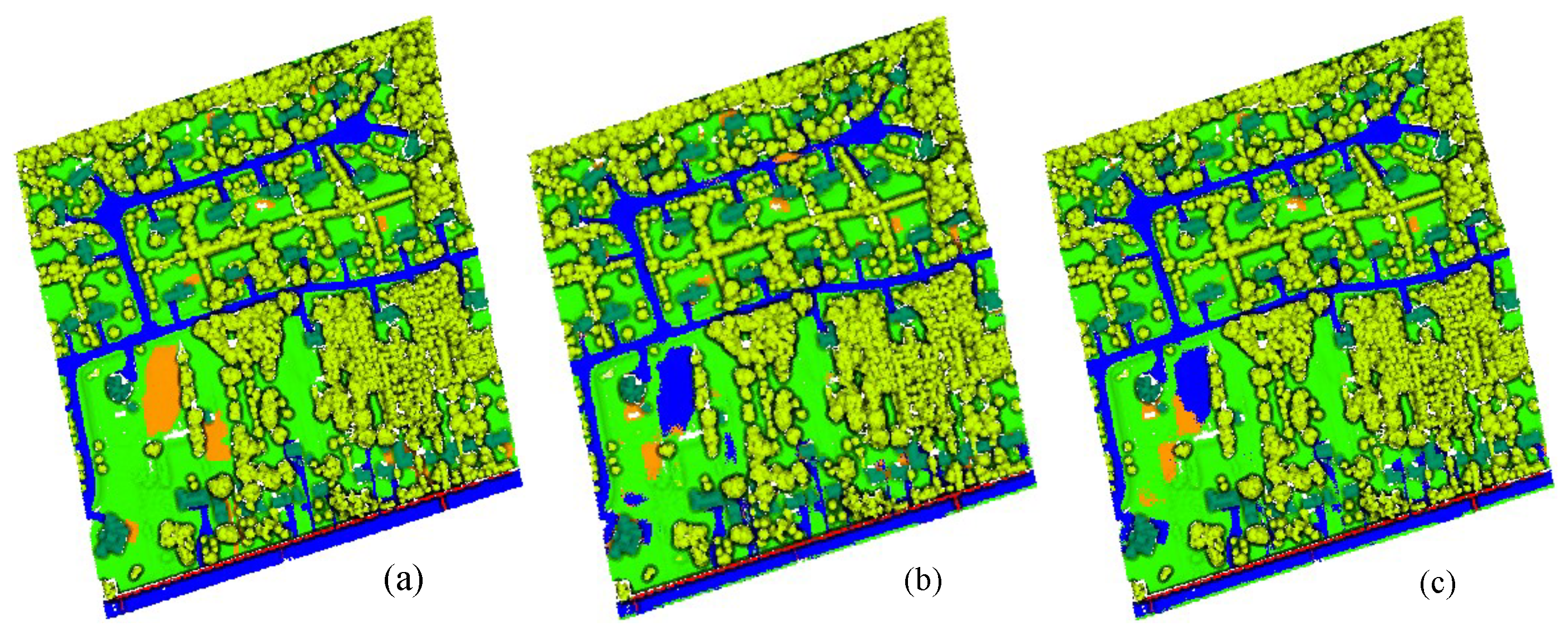
Figure 9.
The ground truth and prediction results for Area_13. (a) Ground Truth. (b) Prediction results of MPT algorithm. (c) Prediction results of MPT+ algorithm.
Figure 9.
The ground truth and prediction results for Area_13. (a) Ground Truth. (b) Prediction results of MPT algorithm. (c) Prediction results of MPT+ algorithm.

Figure 10.
Multispectral point cloud classification results with different neighbor points.


Table 1.
Details of the Titan Multispectral LiDAR system.
| Channel | C1 | C2 | C3 |
|---|---|---|---|
| Waveband | SWIR | NIR | GREEN |
| Wavelength (nm) | 1550 | 1064 | 532 |
| Point distance (points/m) | 2 | 2 | 2 |
Table 2.
Details of Multispectral Point Clouds (# represents the number of points).
| Road (#) | Building (#) | Grass (#) | Tree (#) | Soil (#) | Powerline (#) | ||
|---|---|---|---|---|---|---|---|
| Training | Area_1 | 37,956 | 19,821 | 207,394 | 428,525 | 4549 | 0 |
| Area_2 | 24,594 | 10,408 | 130,884 | 259,930 | 4761 | 809 | |
| Area_3 | 71,175 | 78,587 | 308,337 | 480,545 | 13,713 | 0 | |
| Area_4 | 32,601 | 45,556 | 79,891 | 254,723 | 7070 | 493 | |
| Area_5 | 75,710 | 46,571 | 347,264 | 79,966 | 7189 | 0 | |
| Area_6 | 63,879 | 39,436 | 71,229 | 207,817 | 1703 | 591 | |
| Area_7 | 63,879 | 39,436 | 224,173 | 274,159 | 1268 | 2626 | |
| Area_8 | 70,757 | 25,794 | 254,340 | 342,594 | 6344 | 4561 | |
| Area_9 | 72,570 | 33,754 | 355,467 | 155,838 | 9465 | 2153 | |
| Area_10 | 60,764 | 61,764 | 395,228 | 96,810 | 31,589 | 0 | |
| Total | 573,885 | 401,127 | 2,374,207 | 2,580,907 | 87,651 | 11,233 | |
| Testing | Area_11 | 91,407 | 41,390 | 261,218 | 455,500 | 16,968 | 2533 |
| Area_12 | 94,965 | 40,941 | 367,039 | 252,181 | 6181 | 2859 | |
| Area_13 | 117,994 | 65,040 | 478,454 | 198,248 | 46,380 | 3075 | |
| Total | 304,366 | 147,371 | 1,106,711 | 905,929 | 69,529 | 8467 |
Table 3.
Settings of the network parameters.
| Hyper-Parameters | |
|---|---|
| N | 4096 |
| K | 32 |
| Batch | 32 |
| Epoch | 200 |
| Optimizer | Adam |
| Weight decay | 0.0001 |
| Learning rate | Initial rate 0.001 multiply by 0.7 every 16 epochs |
Table 4.
Prediction results of MPT network (# represents the number of the points).
| Road (#) | Building (#) | Grass (#) | Tree (#) | Soil (#) | Powerlines (#) | |
|---|---|---|---|---|---|---|
| Road | 278,965 | 36 | 20,761 | 6 | 4598 | 0 |
| Building | 712 | 144,159 | 315 | 2033 | 140 | 12 |
| Grass | 26,306 | 963 | 1,056,245 | 3912 | 19,285 | 0 |
| Tree | 99 | 3353 | 4529 | 897,766 | 38 | 144 |
| Soil | 41,468 | 50 | 9037 | 5 | 18,969 | 0 |
| Powerlines | 0 | 2 | 0 | 705 | 0 | 7760 |
| (%) | 74.80 | 94.98 | 92.54 | 98.38 | 20.27 | 89.99 |
| (%) | 80.27 | 97.04 | 96.82 | 99.26 | 44.08 | 98.03 |
| (%) | 91.65 | 97.82 | 95.44 | 99.10 | 27.28 | 91.65 |
| (%) | 85.58 | 97.43 | 96.13 | 99.18 | 33.70 | 94.73 |
Table 5.
Prediction results for the MPT+ network (# represents the number of the points).
| Road (#) | Building (#) | Grass (#) | Tree (#) | Soil (#) | Powerlines (#) | |
|---|---|---|---|---|---|---|
| Road | 278,193 | 1 | 23,161 | 0 | 3011 | 0 |
| Building | 88 | 145,014 | 318 | 1593 | 358 | 0 |
| Grass | 22,063 | 593 | 1,069,583 | 2852 | 11,620 | 0 |
| Tree | 30 | 1196 | 2530 | 902,061 | 24 | 88 |
| Soil | 27,809 | 7 | 13,643 | 41 | 28,029 | 0 |
| Powerlines | 0 | 0 | 0 | 226 | 0 | 8241 |
| (%) | 78.58 | 97.19 | 93.30 | 99.05 | 33.03 | 96.51 |
| (%) | 84.85 | 98.80 | 96.42 | 99.47 | 64.73 | 98.90 |
| (%) | 91.40 | 98.35 | 96.65 | 99.57 | 40.28 | 97.56 |
| (%) | 88.00 | 98.58 | 96.53 | 99.52 | 49.66 | 98.22 |
Table 6.
Comparative results of different methods in the tested areas.
| Model | (%) | (%) | (%) | |
|---|---|---|---|---|
| PointNet [24] | 83.79 | 44.28 | 46.68 | 0.73 |
| PointNet++ [25] | 90.09 | 58.60 | 70.13 | 0.84 |
| DGCNN [19] | 91.36 | 51.04 | 66.17 | 0.86 |
| GACNet [21] | 89.91 | 51.04 | 66.17 | 0.84 |
| RSCNN [20] | 90.99 | 56.10 | 70.23 | 0.86 |
| SE-PointNet++ [26] | 91.16 | 60.15 | 73.14 | 0.86 |
| PCT [55] | 93.55 | 75.87 | 83.03 | 0.90 |
| MPT | 94.55 | 78.49 | 84.46 | 0.92 |
| MPT+ | 95.62 | 82.94 | 88.42 | 0.94 |
Table 7.
Impact of bias on results. The first six columns of values are the of each class.
| Model | Road | Building | Grass | Tree | Soil | Powerline | (%) | (%) |
|---|---|---|---|---|---|---|---|---|
| MPT_w/o_Bias | 72.49 | 90.51 | 92.44 | 97.88 | 5.78 | 86.54 | 74.27 | 93.99 |
| MPT_w/_Bias | 74.80 | 94.98 | 92.54 | 98.38 | 20.27 | 89.99 | 78.49 | 94.55 |
| MPT+_w/o_Bias | 78.51 | 95.66 | 92.61 | 98.62 | 21.13 | 95.55 | 80.34 | 95.13 |
| MPT+_w/_Bias | 78.58 | 97.19 | 93.30 | 99.05 | 33.03 | 96.51 | 82.94 | 95.62 |
Table 8.
Multispectral point cloud classification results with different types of input data. The first six columns of values are the of each class.
Table 8.
Multispectral point cloud classification results with different types of input data. The first six columns of values are the of each class.
| Input | Road | Building | Grass | Tree | Soil | Powerlines | (%) | (%) |
|---|---|---|---|---|---|---|---|---|
| xyz | 38.85 | 87.64 | 75.08 | 97.35 | 1.97 | 83.14 | 64.01 | 86.04 |
| xyz + C1 | 39.19 | 91.34 | 75.27 | 97.80 | 9.22 | 87.16 | 66.67 | 86.10 |
| xyz + C2 | 74.60 | 94.33 | 90.43 | 98.50 | 9.17 | 95.88 | 77.15 | 93.98 |
| xyz + C3 | 46.93 | 88.67 | 79.48 | 97.51 | 8.73 | 83.08 | 67.40 | 87.36 |
| xyz + C123 | 78.58 | 97.19 | 93.30 | 99.05 | 33.03 | 96.51 | 82.94 | 95.62 |
Table 9.
Multispectral Point cloud classification results with different sampling points. The first six columns of values are the of each class.
Table 9.
Multispectral Point cloud classification results with different sampling points. The first six columns of values are the of each class.
| N | Road | Building | Grass | Tree | Soil | Powerlines | (%) | (%) |
|---|---|---|---|---|---|---|---|---|
| 4096 | 78.58 | 97.19 | 93.30 | 99.05 | 33.03 | 96.51 | 82.94 | 95.62 |
| 2048 | 74.89 | 96.57 | 92.77 | 98.75 | 21.64 | 91.31 | 79.32 | 94.81 |
| 1024 | 72.74 | 93.18 | 91.78 | 97.63 | 9.58 | 88.91 | 75.64 | 93.92 |
| 512 | 72.76 | 90.65 | 90.71 | 97.51 | 21.42 | 76.42 | 74.91 | 93.57 |
Table 10.
Multispectral point cloud classification results with different neighbor points. The first six columns of values are the of each class.
Table 10.
Multispectral point cloud classification results with different neighbor points. The first six columns of values are the of each class.
| K | Road | Building | Grass | Tree | Soil | Powerline | (%) | (%) |
|---|---|---|---|---|---|---|---|---|
| 4 | 77.62 | 96.86 | 93.39 | 98.82 | 39.74 | 94.41 | 83.47 | 95.57 |
| 8 | 76.28 | 97.26 | 93.02 | 98.97 | 29.98 | 95.89 | 81.90 | 95.20 |
| 16 | 77.97 | 96.22 | 92.17 | 98.80 | 14.75 | 94.59 | 79.08 | 94.88 |
| 24 | 77.46 | 97.09 | 92.60 | 98.87 | 21.92 | 94.57 | 80.42 | 95.01 |
| 32 | 78.58 | 97.19 | 93.30 | 99.05 | 33.03 | 96.51 | 82.94 | 95.62 |
| 64 | 77.87 | 96.76 | 93.34 | 98.84 | 33.60 | 91.54 | 81.99 | 95.44 |
Table 11.
Multispectral point cloud classification results with different loss functions. The first six columns of values are the of each class.
Table 11.
Multispectral point cloud classification results with different loss functions. The first six columns of values are the of each class.
| Road | Building | Grass | Tree | Soil | Powerlines | (%) | (%) | |
|---|---|---|---|---|---|---|---|---|
| Case 1 | 78.01 | 97.07 | 93.10 | 98.79 | 28.44 | 95.69 | 81.85 | 95.39 |
| Case 2 | 78.58 | 97.19 | 93.30 | 99.05 | 33.03 | 96.51 | 82.94 | 95.62 |
Table 12.
Comparison of computing resources based on Transformer-based networks.
| PCT | MPT | MPT+ | |
|---|---|---|---|
| FLOPs (G) | 502.34 | 467.57 | 14.78 |
| Params (M) | 3.83 | 3.57 | 1.91 |
Table 13.
Semantic segmentation results on S3DIS dataset. The first thirteen rows of values are the of each class.
Table 13.
Semantic segmentation results on S3DIS dataset. The first thirteen rows of values are the of each class.
| Model | PointNet [24] | MinkowskiNet [62] | PAconv [63] | PointTrans [53] | MPT+ |
|---|---|---|---|---|---|
| Ceiling | 88.8 | 91.8 | 94.6 | 94.0 | 92.3 |
| Floor | 97.3 | 98.7 | 98.6 | 98.5 | 98.3 |
| Wall | 69.8 | 86.2 | 82.4 | 86.3 | 84.4 |
| Beam | 0.1 | 0.0 | 0.0 | 0.0 | 0.0 |
| Column | 3.9 | 34,1 | 26.4 | 38.0 | 33.1 |
| Window | 46.3 | 48.9 | 58.0 | 63.4 | 59.3 |
| Door | 10.8 | 62.4 | 60.0 | 74.3 | 65.7 |
| Table | 59.0 | 81.6 | 80.4 | 89.1 | 89.2 |
| Chair | 52.6 | 89.8 | 89.7 | 82.4 | 78.6 |
| Sofa | 5.9 | 47.2 | 69.8 | 74.3 | 74.4 |
| Book | 40.3 | 74.9 | 74.3 | 80.2 | 67.4 |
| Board | 26.4 | 74.4 | 73.5 | 76.0 | 74.7 |
| Clutter | 33.2 | 58.6 | 57.7 | 59.3 | 55.2 |
| (%) | 41.1 | 65.4 | 66.6 | 70.4 | 67.1 |
Publisher’s Note: MDPI stays neutral with regard to jurisdictional claims in published maps and institutional affiliations. |
© 2022 by the authors. Licensee MDPI, Basel, Switzerland. This article is an open access article distributed under the terms and conditions of the Creative Commons Attribution (CC BY) license (https://creativecommons.org/licenses/by/4.0/).
Share and Cite
MDPI and ACS Style
Zhang, Z.; Li, T.; Tang, X.; Lei, X.; Peng, Y. Introducing Improved Transformer to Land Cover Classification Using Multispectral LiDAR Point Clouds. Remote Sens. 2022, 14, 3808. https://doi.org/10.3390/rs14153808
AMA Style
Zhang Z, Li T, Tang X, Lei X, Peng Y. Introducing Improved Transformer to Land Cover Classification Using Multispectral LiDAR Point Clouds. Remote Sensing. 2022; 14(15):3808. https://doi.org/10.3390/rs14153808
Chicago/Turabian StyleZhang, Zhiwen, Teng Li, Xuebin Tang, Xiangda Lei, and Yuanxi Peng. 2022. "Introducing Improved Transformer to Land Cover Classification Using Multispectral LiDAR Point Clouds" Remote Sensing 14, no. 15: 3808. https://doi.org/10.3390/rs14153808
Note that from the first issue of 2016, this journal uses article numbers instead of page numbers. See further details here.