
A Shipborne Photon-Counting Lidar for Depth-Resolved Ocean Observation
by
 , , ,
, , ,
Xue Shen
1,2,3 ,
,
Wei Kong
1,2,3,4,*,
Peng Chen
5,
Tao Chen
1,2,3,4,
Genghua Huang
1,2,3,4 and
Rong Shu
1,2,3,4 1
Key Laboratory of Space Active Optical-Electro Technology, Shanghai Institute of Technical Physics, Chinese Academy of Sciences, Shanghai 200083, China
2
Shanghai Branch, Hefei National Laboratory, Shanghai 201315, China
3
Shanghai Research Center for Quantum Sciences, Shanghai 201315, China
4
University of Chinese Academy of Sciences, Beijing 100049, China
5
State Key Laboratory of Satellite Ocean Environment Dynamics, Second Institute of Oceanography, Ministry of Natural Resources, 36 Baochubei Road, Hangzhou 310012, China
*
Author to whom correspondence should be addressed.
Remote Sens. 2022, 14(14), 3351; https://doi.org/10.3390/rs14143351
Submission received: 12 May 2022
/
Revised: 7 July 2022
/
Accepted: 10 July 2022
/
Published: 12 July 2022
(This article belongs to the Special Issue Remote Sensing of the Sea Surface and the Upper Ocean)
Abstract
:Depth-resolved information is essential for ocean research. For this study, we developed a shipborne photon-counting lidar for depth-resolved oceanic plankton observation. A pulsed fiber laser with frequency doubling to 532 nm acts as a light source, generating a single pulse at the micro-joule level with a pulse width of less than 1 ns. The receiver is capable of simultaneously detecting the elastic signal at two orthogonal polarization states, the Raman scattering from seawater, and the fluorescence signal from chlorophyll A. The data acquisition system utilizes the photon-counting technique to record each photon event, after which the backscattering signal intensity can be recovered by counting photons from multiple pulses. Benefitting from the immunity of this statistical detection method to the ringing effect of the detector and amplifier circuit, high-sensitivity and high-linearity backscatter signal measurements are realized. In this paper, we analyze and correct the after-pulse phenomenon of high-linearity signals through experiments and theoretical simulations. Through the after-pulse correction, the lidar attenuation coefficient retrieved from the corrected signal are in good agreement with the diffuse attenuation coefficients calculated from the in situ instrument, indicating the potential of this shipborne photon-counting lidar for ocean observation applications.
1. Introduction
By emitting laser pulses, oceanic lidar measures the backscattered signals from the water surface, seawater, and sea bottom to realize depth-resolved observation [1,2]. It has become an effective tool in many fields, such as underwater target detection and identification [3,4,5], shallow water mapping [6,7,8,9,10], laser-induced fluorescence [11,12], and surface roughness measurements [13,14]. In the field of ocean ecology research, oceanic lidar has also been demonstrated to have the ability to distinguish plankton content at different depths [15,16].
Due to the strong attenuation property of seawater, the oceanic lidar signal is attenuated by several orders of magnitude in several tens to hundreds of nanoseconds. When amplifying the signal and converting it using analog-to-digital circuits, the weak signal at greater depth is disturbed by oscillations and long-lasting tails generated by strong signals from water surface reflection and shallow water backscattering [17,18]. The after-pulse effect of the detector and its amplifier circuit degrade the linearity of the signal, especially at deep depths, and should be carefully calibrated in the laboratory and corrected during data processing. For example, the echo signals of CALIOP were corrected by measuring the land surface return to build a deconvolution kernel function, in order to obtain a pure seawater backscatter [19,20]. Li et al. corrected the after-pulse response of an airborne oceanic lidar by measuring the after-pulse count occurrence probability distribution for input signal pulses of varying intensities in the laboratory [21].
In contrast to analog-to-digital conversion, the photon-counting technique records the arrival time of each photon, while the gain of the detector is set extremely high. This technique will fail when the echo is too strong, in which case the circuits cannot resolve adjacent photon events. Therefore, photon-sensitive lidars generally have relatively low single-pulse energy and a high repetition rate. For example, the Advanced Topographic Laser Altimeter System (ATLAS) aboard NASA’s Ice, Cloud, and Land Elevation Satellite-2 (ICESat-2) has a single-pulse energy of only about 48–170 μJ [22]. Given its high repetition rate of 10 kHz, Lu et al. accumulated the recorded photons from thousands to tens of thousands of shots into different range bins, resulting in a state-of-the-art oceanic lidar signal decay with depth [23]. The signal of ATLAS has excellent linearity without the ringing phenomenon, demonstrating that the photon-counting technique has advantages for underwater signal recovery.
In this paper, based on the photon-counting technique, a shipborne oceanic lidar was developed at the Shanghai Institute of Technical Physics, Chinese Academy of Sciences. Different from typical lidar, which acquires the lidar scattered signal using analog-to-digital conversion circuits, this lidar is based on the time-correlated single photon-counting (TCSPC) technique [24,25], which measures the time difference between the emitted laser pulse and the photon events received by the detectors. By collecting histogram statistics of the photon events from multiple laser pulses, the oceanic lidar’s intensity curve can be retrieved, which decays with depth. Compared with the analog-to-digital conversion circuits, the photon-counting method is immune to the ringing effect of the amplification circuits, therefore the signal still has better linearity over several orders of magnitude. The high linearity also helps us to resolve the weak after-pulse effects in photon-counting lidar, which are mainly caused by the laser pulse profile and the non-ideal recovery of the detector. In this paper, we discuss the sources and the method for removal of the signal’s after-pulse in detail, prior to the data application.
2. Instrument and Methods
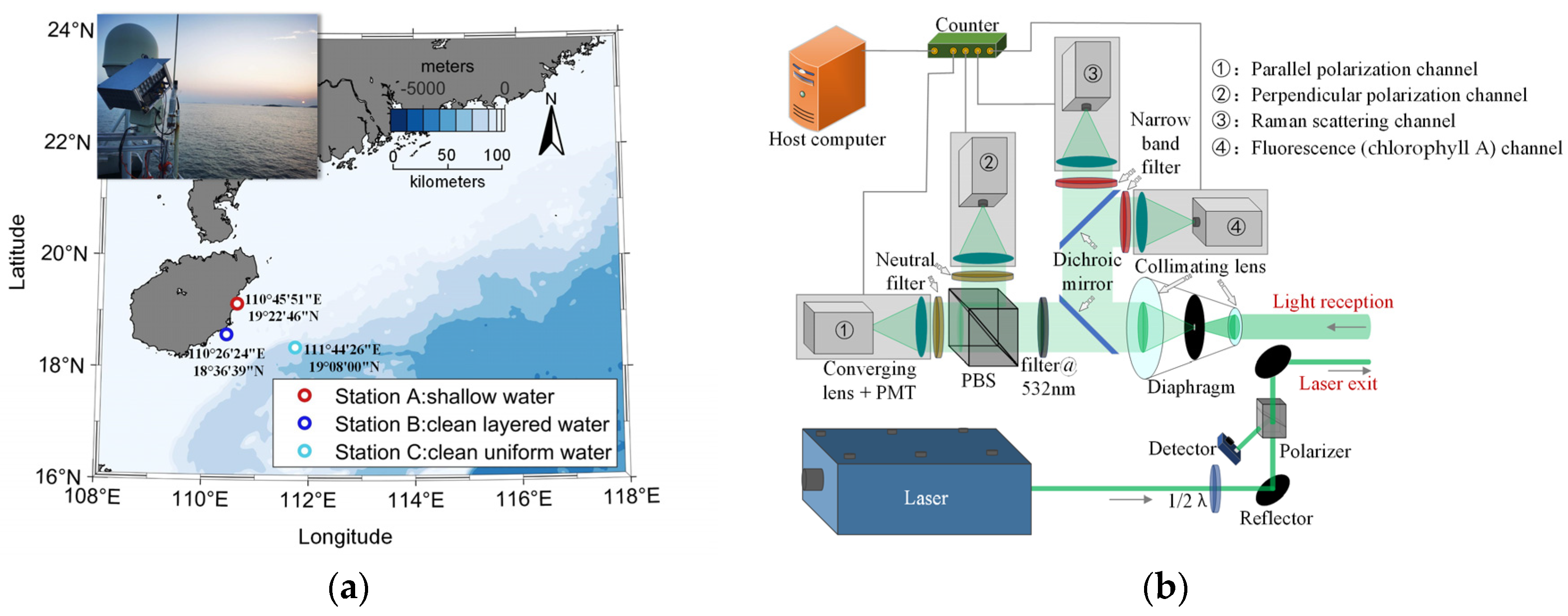
The 532 nm micro-pulse shipborne lidar we developed is capable of detecting the Raman scattering from seawater, the fluorescence signal from chlorophyll A, and elastic signals at two orthogonal polarization states simultaneously. In September 2020, this lidar participated in the joint voyage of the National Key Research and Development Program Lidar organized by the Second Institute of Oceanography, Ministry of Natural Resources. This instrument is mounted on a dual-axis gimbal on a ship and tilted at a certain angle to steer the beam direction to the seawater, as shown in the upper left corner of Figure 1. The ship is also equipped with relevant in situ sensors, such as the HydroScat-6P and the ac-spectra. Stations A to C marked on the map in Figure 1a are the locations of data collection, as described in the following text. Figure 1b shows the structure of the lidar; it is composed of a transmitter, receiver, and data acquisition system. Furthermore, the major specifications of the lidar are listed in Table 1.
2.1. Transmitter
The transmitter emits a highly linearly polarized pulsed laser into the seawater. It is composed of a laser, a polarizer, a half waveplate, a reference pulse detector, and several reflection mirrors. The homemade fiber laser-pumped green laser has the same structure as described in our previous paper [26]. It emits a short-pulse laser with a wavelength of 532.1 nm. A half waveplate is used to rotate the polarization state to be horizontal to the mounting surface. Then, a polarizer with an extinction ratio larger than 10,000:1 is used, in order to improve the polarization purity of the emitted laser. In the transmitter, a reference detector that collects the residual laser in the reflection direction of the polarizer is used to generate a start signal for the data acquisition system.
2.2. Receiver
The receiver collects the scattered signal from the seawater with a lens, having a diameter of 4 mm and a focal length of 8 mm. Then, a diaphragm with a diameter of 0.5 mm is placed at its infinity focus, in order to constrain the receiving field of view to 62.5 mrad. The receiving field of view is much larger than the laser divergence angle to collect multiple scattering signals, considering the diffusion of the laser beam underwater. A lens with a focal length of 35 mm is placed after the diaphragm to collimate the echo. Then, the signal is separated into elastic, Raman, and fluorescence channels by two dichromatic beam splitters. The filter bandwidths of the two inelastic channels are 20 nm and 30 nm for the broad spectral features of Raman and fluorescence spectra, respectively. Therefore, the solar background radiation in the daytime is too large at these two channels to obtain high-quality signals. In the elastic channel, a bandpass filter with a bandwidth of 0.6 nm is used to filter the out-of-band noise. The elastic signal is then separated by a polarization beam splitter (PBS) into components that are parallel and perpendicular to the polarization state of the transmitted laser. The PBS is specially coated to achieve high polarization extinction ratios at both channels. The receiver then focuses the signals of the four channels onto photomultiplier tubes (PMTs).
The PMTs are manufactured by Hamamatsu Inc. in Japan, with the model number H10721-20. The gain of the PMTs should be adjusted to exceed 106, in order to be able to distinguish a single photon event. The output signals of the PMTs are then amplified by a circuit to an amplitude that can be recognized by the data acquisition system.
2.3. Data Acquisition System
The four-channel data acquisition system was manufactured by Siminics in China, with the model number FT1040. It measures the time difference between the emitted laser pulse signal from the reference detector and the amplified photon pulses from the PMTs with a time resolution of 64 ps. The system has a dead time of 10 ns, which means that it can only distinguish two photon events with a time interval greater than 10 ns. Therefore, when the signal intensity is so high that the average photon-counting rate—which is defined as the number of photons detected per second—reaches tens of megahertz, a linear photon distribution will result in an obvious non-linear response. To reduce the influence of such a non-linear response caused by saturation, several neutral density filters are added in the elastic channels, in order to weaken the signal intensity near the water surface. Even so, there will still be some non-linearity in the signal near the water surface.
2.4. Lidar Signal Pre-Processing Method
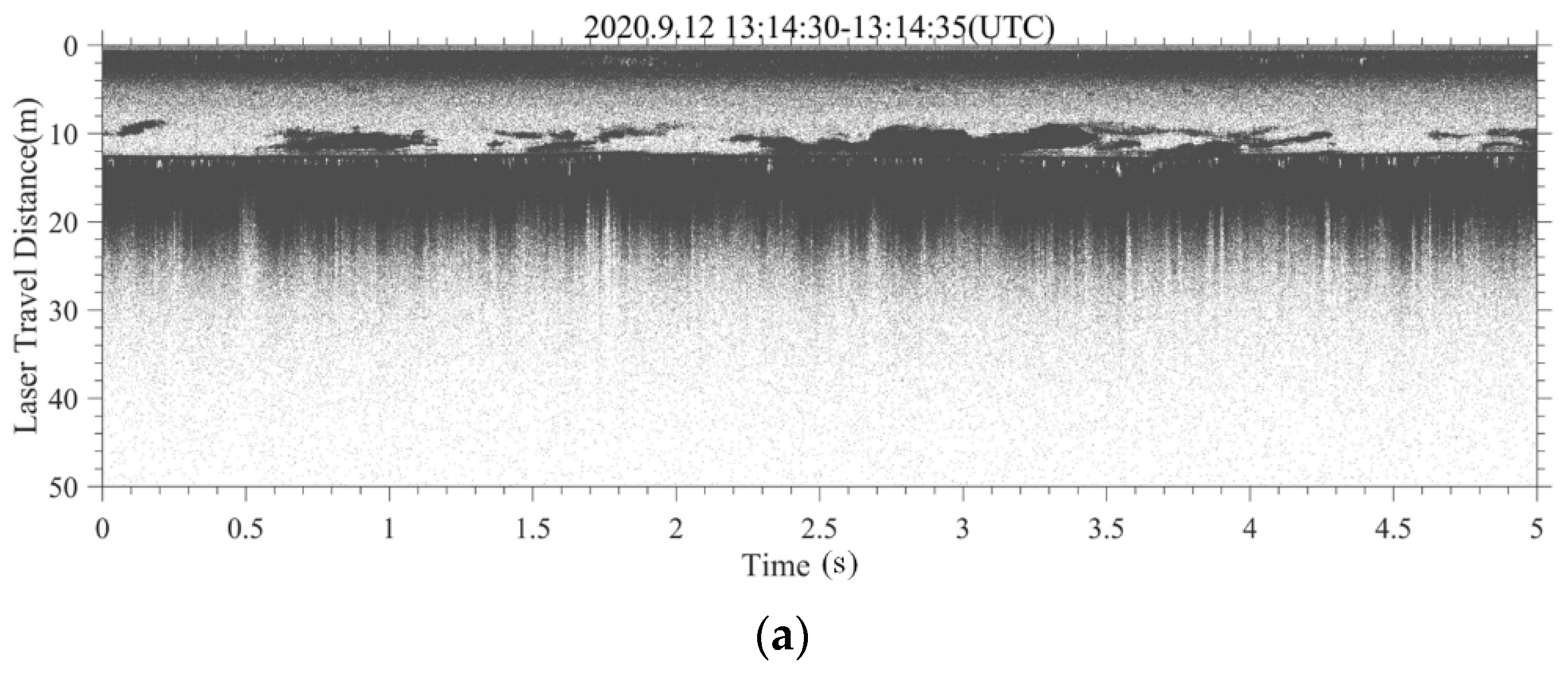
Different from the analog-to-digital conversion detection technique, the raw data collected by the photon-counting technique consist of the arrival time of each photon event. Therefore, a different method for pre-processing the photon-counting signal should be proposed. Figure 2a shows the typical raw data at the parallel polarization channel. Each gray point in this figure represents a photon event. As the depth increases, the density of photon events becomes lower, which indicates that the signal intensity becomes lower. The horizontal axis is the laser pulse emission time, and the vertical axis is the distance corresponding to the photon arrival time.
A two-dimensional grid was designed, with resolutions of 20 ms and 0.0384 m for the pulse emitting time and distance axes, respectively. Then, the photon number in each pixel was counted. The statistical results are shown in Figure 2b, which exhibits the distribution of atmospheric aerosols above the water surface and the underwater backscattered signals that decay with depth. The fluctuating water–air interface caused by the ship shaking can be clearly distinguished in this panel. By searching for the position of maximum signal intensity, the distance of the water surface for every 20 ms profile can be retrieved; this is set as the zero-depth position. Then, the profiles at 30 s are aligned to the zero-depth position and accumulated into a single profile with high signal-to-noise ratio. Figure 2c shows the variations in the high signal-to-noise ratio signal over 6 h with a time resolution of 30 s and underwater distance resolution of 0.0289 m. The variations in signal intensity caused by underwater plankton activity can also be distinguished.
2.5. In Situ Measurements
The in situ data used in this paper for comparison with oceanic lidar were provided by HydroScat-6P and ac-spectra. The HydroScat-6P is a self-contained instrument for measuring optical backscattering at six different wavelengths in natural waters. The data products of HydroScat-6P include the scattering coefficients at 140° for six different wavelengths, and the backscattering coefficients corresponding to the six wavelengths can be obtained through correction using the built-in software. Considering that the detection wavelength of the lidar is 532 nm, the adjacent wavelengths detected by the HydroScat-6P are 510 nm and 590 nm, respectively. Therefore, the 532 nm backscattering coefficient for comparison was generated by linear interpolation of the backscattering coefficients at 510 nm and 590 nm. The ac-spectra performs concurrent measurements of the water’s attenuation and absorption characteristics by incorporating a dual-path optical configuration in a single sensor. The direct data products of ac-spectra include absorption coefficients and beam attenuation coefficients at 532 nm. It should be noted that, due to the multiple scattering of seawater, the lidar attenuation coefficient cannot be equal to the beam attenuation coefficient measured by ac-spectra directly.
After considering multiple scattering, it is necessary to calculate the diffusion attenuation coefficient, Kd, according to the absorption and backward-scatter coefficients, which are used for comparison with the retrieved lidar attenuation coefficient. The following formula was used to calculate Kd [27]
where a is the absorption coefficient at 532 nm calculated by the ac-spectra, and bb is the backward-scatter coefficient at 532 nm calculated by the HydroScat-6P. When the influence of pure seawater has been corrected in the in situ measurement results, the diffusion attenuation coefficient of pure seawater must be considered before comparison. The diffusion attenuation coefficient of pure seawater is assumed to be 0.045 m−1 [15].
3. Experimental Results and Analysis
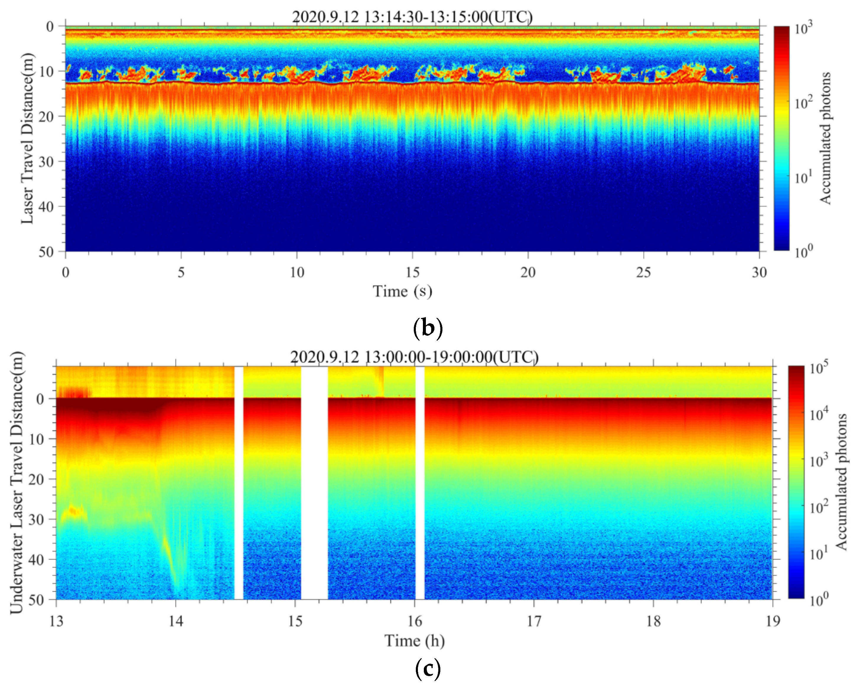
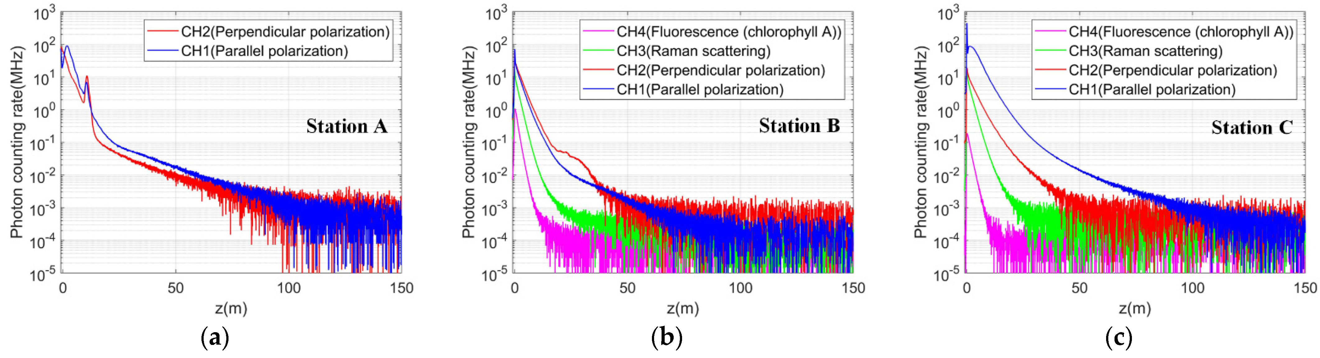
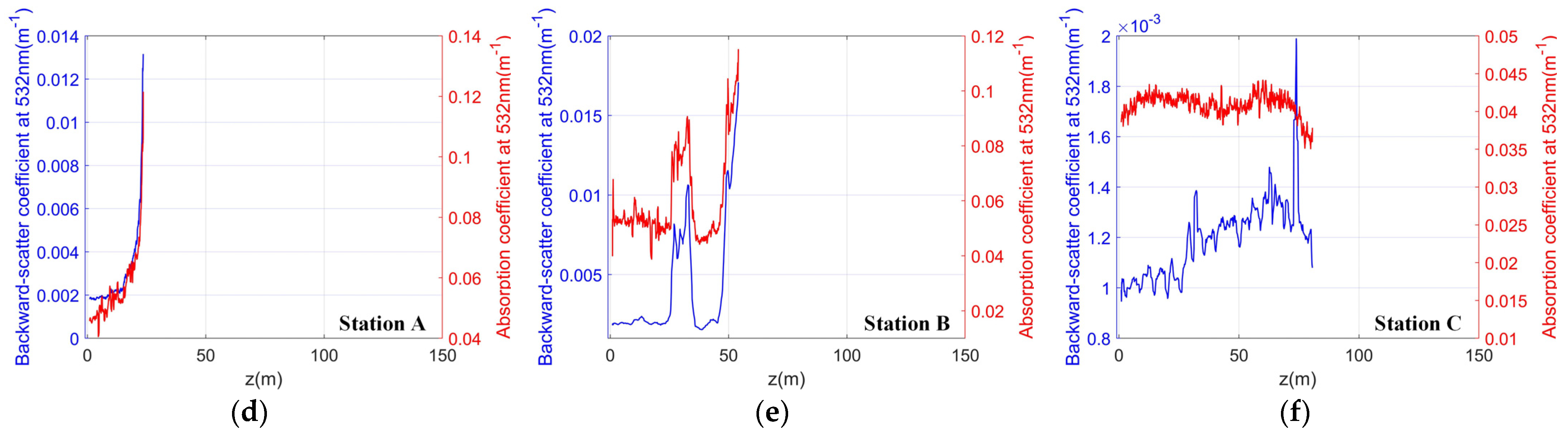
Figure 3a–c shows the accumulated profiles with an accumulation time of 30 s at stations A, B, and C, which correspond to locations characterized by shallow water, deep water with layered plankton, and deep water with homogeneous plankton, respectively. The underwater distance resolution of the signals is 0.0289 m. The vertical axis is represented by the photon-counting rate, PCR, which is calculated from the accumulated photons AP using the formula PCR = AP/(N × Tgate), where Tgate is the time corresponding to the distance gate width of 0.0289 m, which is 256 ps for this profile; and N is the number of the emitted laser pulses. In 30 s, approximately 6 million pulses are fired. At all stations, the state-of-the-art signals accumulated by the photon-counting method have no oscillation effects, as occurs with an analog signal. The in situ measured backscatter coefficient and absorption coefficient are presented in Figure 3d–f. At station A of shallow water, the backscatter and absorption coefficient increase to a maximum near the bottom. At station B, the in situ measured local maximum around 30 m indicated that there is a plankton enrichment. At the same depth, the accumulated signal at the perpendicular polarization channel also shows an obvious bulge. At station C, the in situ measured absorption and backscatter coefficient are the smallest among the three stations, which is consistent with the slow signal decay speed with depth. Moreover, the accumulated photon number at station C is approximately 25 at 100 m while the range bin is 0.0289 m. Then the signal to noise ratio that can be simply calculated from the square root of the accumulated photon number AP is approximately 5, which means that the signal variation can still be resolved from the noise.
For the elastic channel, the lidar signal from ocean backscattering can be expressed as [18]
where z is travel distance underwater; C is a system constant that includes the laser energy, optical efficiency, detector efficiency, attenuation occurring in the atmosphere between the lidar and the surface, and so on; n is the refractive index of seawater; H is the distance of the instrument from the laser spot at water surface; β is the oceanic backscatter coefficient; and αsea is the lidar attenuation coefficient. Although multiple scattering cannot be negligible under the strong scattering characteristics of seawater, Equation (2) can still be written in the form of a single scattering approximation by introducing the lidar attenuation coefficient [28,29]. The lidar attenuation coefficient has a dependency on the water surface spot diameter with respect to the receiving field and depth. It varies from the beam attenuation coefficient c to the diffuse attenuation coefficient Kd [18]. For a narrow field of view or signal in shallow water, the lidar attenuation coefficient is approximately equal to c, as the single scattering effect dominates, while it is close to Kd when the multiple scattering effect dominates.
In the case of water with homogeneous plankton distribution, the backscatter coefficient β and the attenuation coefficient α can be considered to be constants. In this case, the lidar signal shows an exponential attenuation trend, and the slope method can be used to solve the attenuation coefficient. If the lidar signal after distance correction can be expressed as , α can be calculated using the differential form
Generally, the lidar attenuation coefficient of homogeneous water is calculated using the Least-Squares Fitting method at a low signal-to-noise ratio. This slope method for the atmospheric lidar data retrieval is only suitable for homogeneous water, and will fail if the seawater has layered characteristics.
According to Figure 3, the peak value at zero depth is caused by the strong water surface specular reflection when the laser beam is exactly normal incident on the wave surface. This is reduced at the perpendicular polarization channel, due to the linear polarization characteristics of the emitted laser. At the parallel polarization channel, the specular backscattering reflection is saturated, resulting in a dip behind the peak due to the 10 ns dead time of the acquisition system. Then, the signals exponentially decay with depth to 150 m in the elastic channels. For the Raman channel and the fluorescence channel, which are in contrast to the elastic channels, the backscattering signals are weaker and lack weakly attenuated long-lasting tails. Additionally, they decay faster as seawater has stronger absorption attenuation coefficients at 650 nm and 685 nm [30]. As shown in Figure 3, at all three stations, the elastic signals decayed with depth to nearly 150 m, even at station A, with an underwater depth of only around 10 m. As these long-lasting tails are only contained in the elastic scattering channel, they also exist in the area without oceanic scattering, so we infer that the long-lasting tails appear to originate from non-oceanic scattering.
There are two hypotheses to explain these long-lasting tails. One is the instrument transient response of the photon-counting lidar, which is mainly due to the after-pulse effect of the laser and the detector. The other is the atmospheric scattering, where the water surface acts like a mirror with weak reflectivity. For the ultra-sensitivity of the photon-counting lidar system, the atmospheric scattering signal, which has undergone secondary water surface specular reflection, may be as strong as the seawater scattering in deep water. Considering the difference between the inelastic scattering channel and the elastic scattering channel at the receiving wavelength, these two hypotheses do not contradict. As for the explanation of the instrument transient response, as the wavelength of the laser reflected by the water surface is 532 nm, there is no strong reflection signal at zero depth in the Raman and fluorescence channels and, so, there is no after-pulse.
3.1. Instrument Transient Response
The instrument transient response has been reported in various oceanic lidar systems [14,15]. For example, two small secondary pulses several tens of nanoseconds after the transmit pulse of its laser have been reported for the ATLAS signal. Non-ideal recovery of the detectors in land surface return has also been reported for the CALIOP signal [31]. In summary, the transient response of a lidar instrument can basically be attributed to the laser pulse distribution and the response curve of the detector. It can usually be calibrated and removed through deconvolution, by accumulating the land surface return.
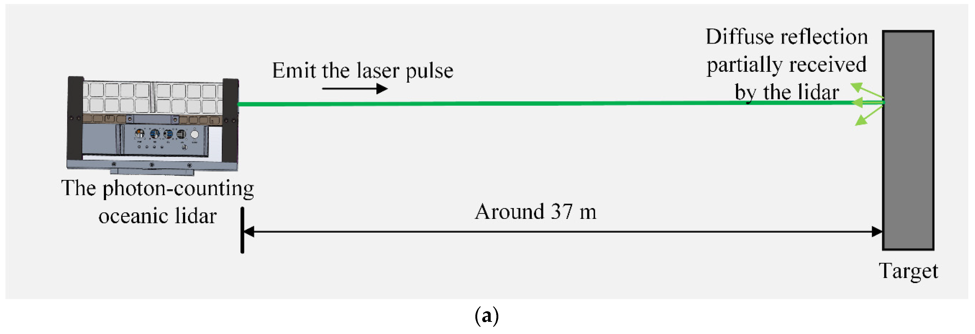
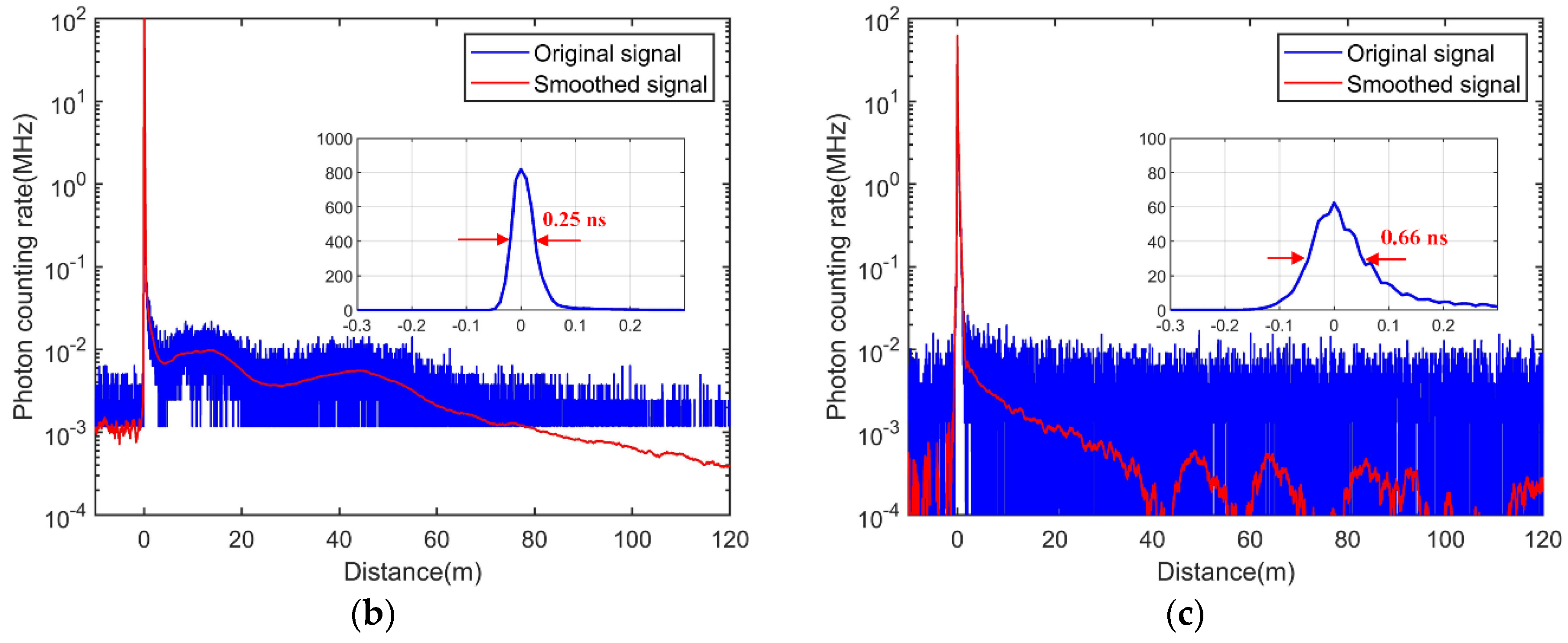
To construct the land surface return of our instrument, a laboratory experiment was conducted to determine the instrument transient response. As shown in Figure 4a, the lidar was pointed to the wall to evaluate the instrument response. Figure 4b,c show the accumulated signals of multiple pulses in logarithmic coordinates at both elastic channels. The horizontal axis is the distance in meters, while the vertical axis is the photon-counting rate. The position of the wall was set to zero. The blue curves are the original signals, while the red curves are the range-smoothed signals.
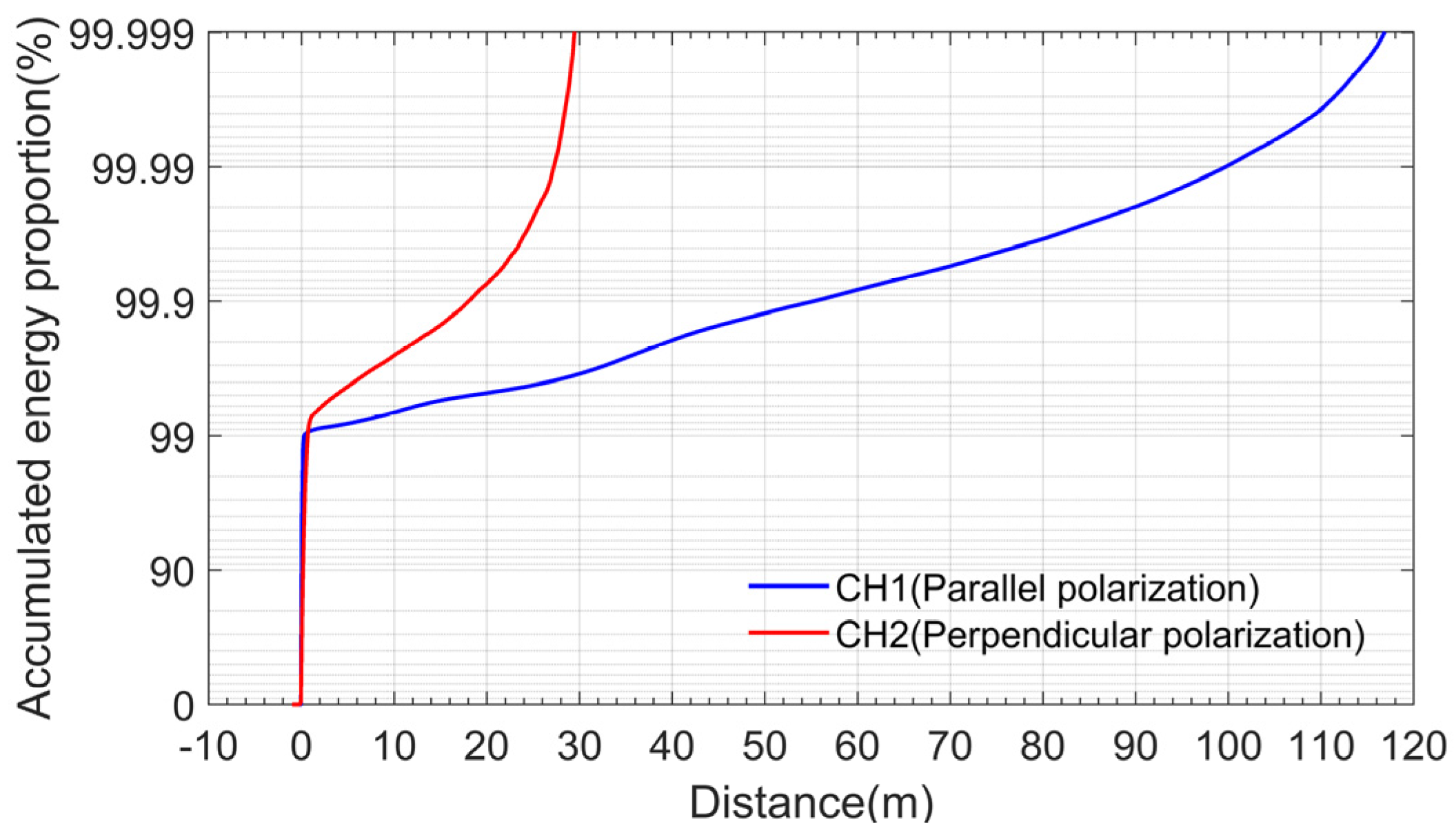
The signal of the hard target is the convolution of the laser pulse shape and the receiver response [32,33,34]. Figure 4 shows that it decreases by at least four orders of magnitude in only approximately 10 ns (or a distance of 1.5 m). The full widths at half maximum are 0.25 ns and 0.66 ns for the parallel polarization channel and the perpendicular polarization channel, respectively. At the parallel polarization channel, the received photons are more concentrated, as the signal is saturated with a peak photon-counting rate exceeding 100 MHz. Similar to the actual test situation, as the laser is linearly polarized, the perpendicular polarization signal is weaker than the parallel one. Thus, the perpendicular channel better reflects the instrument transient response. The width of 0.66 ns at the perpendicular polarization channel is larger than the laser pulse width result of 450 ps for a high-speed detector in previous work [26]. Further analysis of the influence of strong reflections from the water surface on the detection was carried out. We calculated the proportion of pulse energy F(z) after different distances as follows
where p(z) is the instrument transient response. F(z) is shown in Figure 5. The intensity of the strong transient response dropped by four orders of magnitude within tens of nanoseconds after the water surface, lasting up to 100 m in the tail of the parallel polarization channel and up to 40 m in the tail of the perpendicular polarization channel. Even in the parallel polarization channel, the entire tail intensity after less than 1 m underwater only accounted for about 1% of the intensity at the peak position of the pulse; indicating that, under the convolution effect, strong peak position mainly contributes to the long tail, rather than other positions. Then, it can be shown that the after-pulse of the signal tested on the wall can directly characterize the components of the instrument transient response in the oceanic lidar observation. According to Figure 4, after a certain depth, the instrument transient response is similar to a form of exponential decay, such that it can be removed according to the fitting method. Further analysis of its numerical range showed that, in relatively clean seawater (as at Stations B or C) with a depth of 30–50 m, the transient response of the instrument is comparable to the magnitude of the seawater scattering signal. Therefore, in ocean exploration at approximately this depth, the disturbance of the transient response of the instrument cannot be ignored. As the depth increases or the seawater diffusion attenuation coefficient increases, the disturbance of the transient response of the instrument increases.
3.2. Specular Reflection Effect
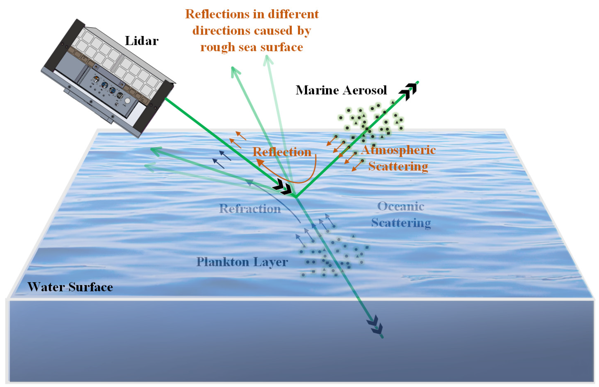
As the shipborne photon-counting lidar can detect deeper seawater with weaker oceanic backscatter, the possibility of interference from weak atmospheric backscatter of specular reflection is not negligible. The sea surface can be treated as a mirror with weak reflectivity, such that the reflected beam interacts with atmospheric aerosols and molecules. The atmospheric backscatter is then reflected by the water surface before entering the lidar receiver. Figure 6 demonstrates this atmospheric backscattering process due to specular reflection by the water surface. In the time domain, the atmospheric backscatter from the specular reflection and the oceanic backscatter are superimposed.
We conducted a simulation of this specular reflection effect, in order to evaluate its influence on oceanic backscatter signal. The elastic lidar signal from ocean backscattering can be expressed by Equation (2). For the specular reflected atmospheric scattering, the oceanic lidar can be treated as a system that observes the atmosphere through a mirror with weak reflectivity, such that the atmospheric backscattering signal can be simply written as
where R is the specular reflectance of the water surface; the subscripts 1 and 2 denote the first and second reflections, respectively; and βatm and αatm are the atmospheric backscatter coefficient and extinction coefficient along the laser irradiation track, respectively.
Equations (2) and (5) can be combined to evaluate the intensity comparison between oceanic and atmospheric backscatter signals. The distance between the lidar and the water surface laser spot H was set as 15.32 m, which was consistent with the experiment. The atmospheric and oceanic optical parameters can be estimated according to the model data or the measurements of other researchers.
In this simulation, the oceanic lidar attenuation coefficient αsea was simply assumed to be the diffuse attenuation coefficient Kd. At a laser wavelength of 532 nm, Kd ranges from 0.05 m−1 for the nearly pure seawater to approximately 0.2 m−1 for the coastal nutrient-rich seawater. Churnside et al. have described the relationship between the lidar extinction-to-backscatter ratio and the chlorophyll concentration [35]. In this research, for seawater with a diffuse attenuation coefficient of less than 0.2 m−1, the lidar extinction-to-backscattering ratio was close to 100 sr, which can be used as a reference for calculation of the backscatter coefficient. Therefore, we set the oceanic backscatter coefficient β to be αsea divided by 100 sr.
Just above the sea surface, the atmospheric extinction is mainly due to marine aerosols. At a given parameter of meteorological visibility V, the atmospheric extinction coefficient αatm can be written as [36]
The lidar extinction-to-backscattering ratio of marine aerosols usually ranges from 22 sr to 32 sr, depending on the wind speed at the sea surface [37]. We used a median value of 27 sr in this simulation. The atmospheric backscattering coefficient βatm was set as αatm divided by 27 sr. At the same time, to simulate the gradient distribution of marine aerosols above the sea surface, the backscatter coefficient βatm decayed at a rate of 10−2 km−1 sr−1 per kilometer [38].
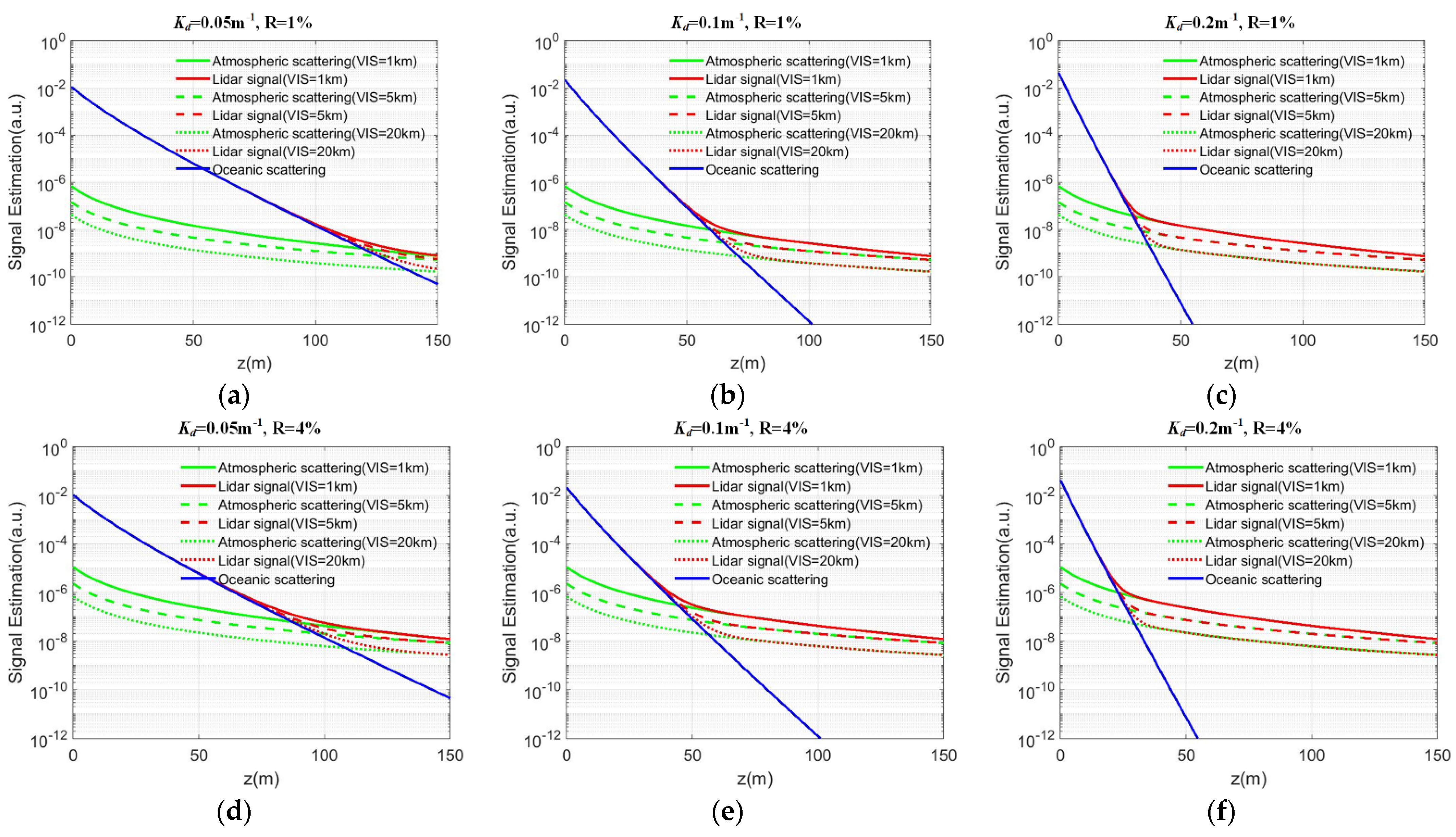
Under the simplest assumption that the sea surface is completely calm, the reflectivity can be calculated by the Fresnel equation. The reflectivity ranges from nearly zero for p polarization at Brewster’s angle to several percent for s polarization at the incident angle of dozens of degrees; however, in an actual marine environment, the waves fluctuate all the time. As shown in Figure 6, the rough sea surface driven by the wind will cause the relative position of the incident laser light to change with the sea surface, thus causing reflections in different directions. Figure 6 only shows the atmospheric scattering path in one reflection case; in fact, the interference of the atmospheric scattering of specular reflection is due to the superposition effect from different reflection paths. Therefore, once the angle between the incident laser and the normal direction of the wave changes, the specular reflectivity will change with the polarization direction of light. This variation in specular reflectance R is coupled with factors, such as the laser pointing angle, the wind-driven oceanic surface waves, the polarization state of the emitted laser, and the polarization direction of the lidar receiver, which make it difficult to assess accurately; however, it is not difficult to define the scope of its change. The maximum reflectivity is given by the s polarization state, which was calculated to be about 4.26%, and the minimum reflectivity is close to 0, given by the p polarization state. For simplicity, we used reflectivities of 1% and 4% to evaluate the signal difference. Finally, we obtained the influence of atmospheric scattering due to specular reflection on ocean scattering, as shown in Figure 7.
In Figure 7, the comparison of atmospheric and oceanic scattering under different atmospheric visibility, marine eutrophication level, and average specular reflectivity of the sea surface is shown. Regardless of completely pure seawater, for most seawater conditions, the oceanic signal below 20–30 m will be affected by atmospheric scattering, especially for the case of fast seawater attenuation and high sea surface reflectivity. The shape of the simulated lidar signal tail superimposed with the atmospheric scattering of the specular reflection also showed an exponential decay trend. As the visibility decreases or the reflectivity increases, the specular reflection effect will increase; however, even with a relatively clean atmosphere (VIS = 20 km) or when the reflectivity of the sea surface is not too high (R = 1%), the influence of both cannot be ignored. In addition, for the depolarization channel, the influence from atmospheric scattering is relatively weak. This is because the depolarization effect of marine aerosol is generally weak.
3.3. After-Pulse Removal Method
The instrumental and non-instrumental effects could both potentially explain the abnormal decay properties of underwater signals. Considering that the interference signals have exponential decay characteristics, it is feasible to extract the after-pulse interference by curve fitting. We conducted an analysis at a station with a homogeneous distribution of plankton, in order to evaluate the after-pulse extraction method.
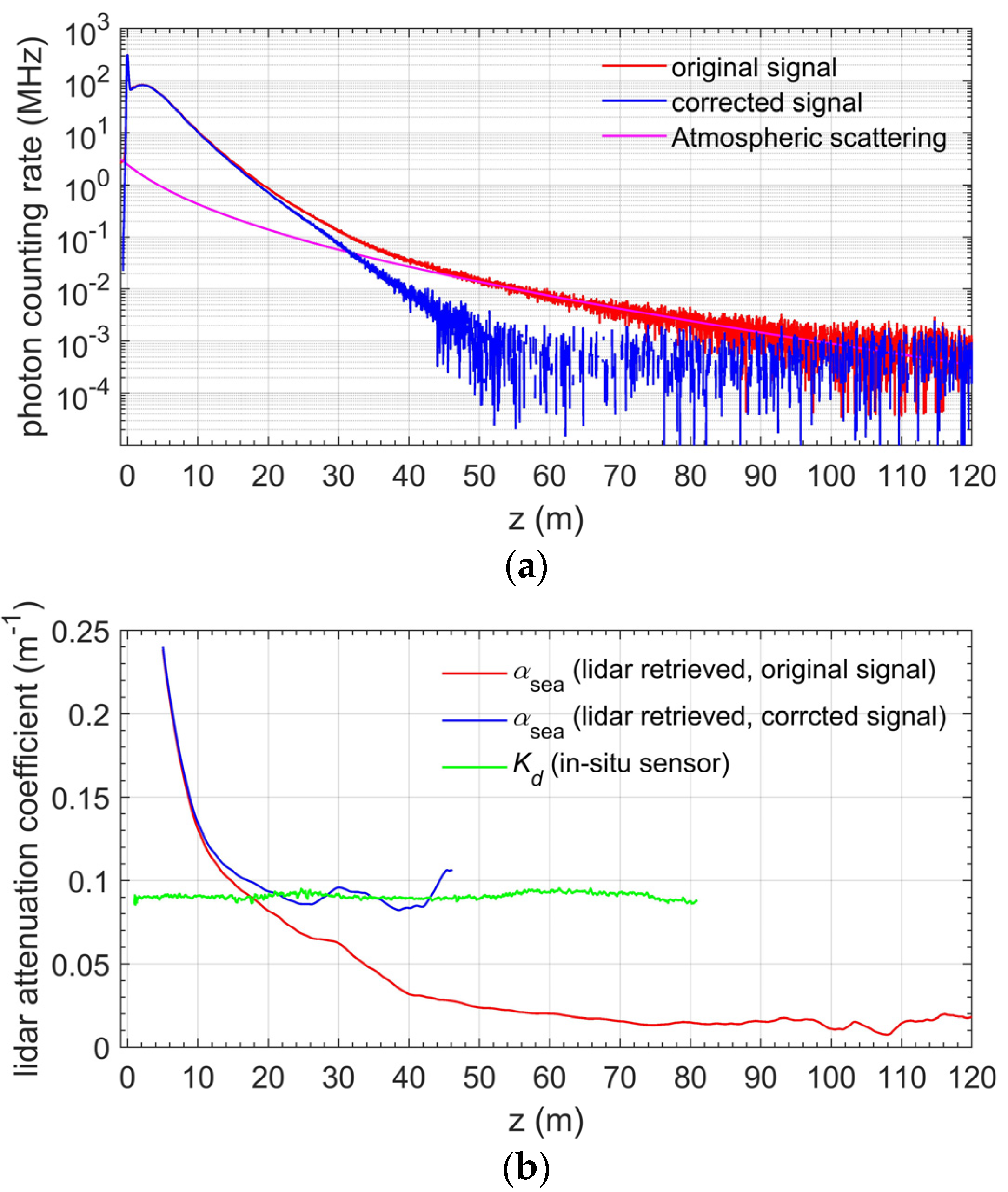
Figure 8 shows the accumulated profile and the retrieval results at the station with homogeneous plankton distribution. In homogeneous seawater, it can be considered that the backscatter coefficient β is depth-independent. Therefore, the lidar signal shows an exponential attenuation trend, and the slope method described in Equation (3) can be used to solve the lidar attenuation coefficient. The red lines in Figure 8a,b represent the original signal and the lidar attenuation coefficient without correction, respectively. Due to signal non-linearity near the water surface, the lidar signal at 0–5 m was not used for retrieval. As for the uncorrected original signal, the lidar attenuation coefficient varied from 0.23 m−1 near the water surface to approximately 0.012 m−1 at an underwater distance exceeding 100 m. At greater depths, it is significantly smaller than the diffuse attenuation coefficient Kd measured by in situ sensors. Such a small attenuation is also far less than the Kd of pure water (0.045 m−1), implying that the original signal has a large deviation from the actual situation, caused by the after-pulse effect. Moreover, the lidar attenuation coefficient showed a downward trend from 10 m to 20 m. The reason for this phenomenon is that the lidar attenuation coefficient gradually approaches the diffuse attenuation coefficient from the beam attenuation coefficient, due to the receiving field of view of the lidar being too small. This phenomenon has been reported in previous simulations and experiments considering oceanic lidar [39].
According to the original signal, we found that the signal after 80 m had an approximately invariant attenuation speed. Considering the change in the ocean scattering intensity caused by multiple scattering, it was confirmed that the signal at this location has no influence of seawater scattering. In addition, as the attenuation of pure seawater at 532 nm reached 0.045 m−1, according to the previous analysis, the seawater scattering continued to decay after 50 m and rapidly attenuated below the after-pulse level, illustrating that the strongly attenuated ocean scattering after 80 m is so weak that it can be neglected. Therefore, the signal greater than 80 m is completely caused by the after-pulse, and can be used as a fitting basis. According to the analysis in Section 3.1 and Section 3.2, both after-pulse effects were characterized by exponential decay. Therefore, we conducted exponential fitting to remove the after-pulse effect. The magenta curve in Figure 8a represents the curve fitted by the signal from 80 m to 120 m. We obtained the pure oceanic backscatter signal by subtracting the fitted curve, represented by the blue line in Figure 8a. The corrected backscatter signal decayed from the sea surface to nearly 50 m underwater. The blue line in Figure 8b represents the retrieved lidar attenuation coefficient from the corrected signal. The corrected lidar attenuation coefficient was close to Kd (green line) calculated from the in situ sensors at an underwater distance greater than 20 m, thus demonstrating that the fitting removal process reduces the signal distortion caused by the instrumental and non-instrumental after-pulse effect. At underwater depths of between 20 m and 50 m, the retrieved lidar attenuation coefficient has a maximum deviation from the in situ measurement of approximately 20%.
3.4. Other Correction Results
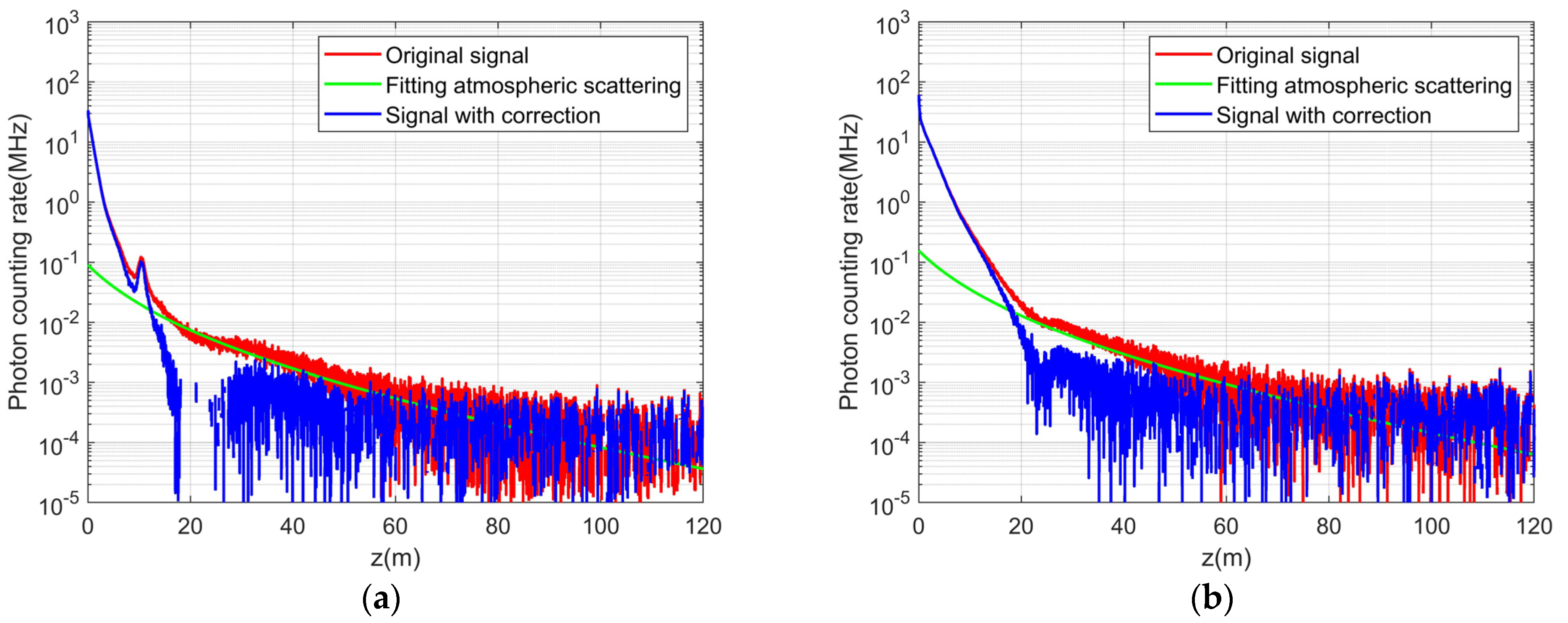
To illustrate the effect of the removal method, after-pulse correction was performed on the data from shallow water and seawater with layered plankton, the results of which are shown in Figure 9. The red line is the original lidar signal, and the blue line is the signal after removing the after-pulse interference. For the shallow water at station A, it can be seen that there was no obvious interference behind the seabed in the signal after correction. For station B, the plankton layers were more conspicuous after correction, which indicates that the after-pulses mask the layered information. Thus, it is necessary to correct the after-pulse effect of the oceanic lidar signal. However, as the backscatter coefficient β is not homogeneous, the slope method is not applicable in seawater with layered plankton. It has been reported that the accurate retrieval of layered seawater optical properties can be carried out by means of high-spectral-resolution lidar or Raman lidar [28,40,41,42]. Subsequent hardware improvements will be made to improve the Raman scattering receiving efficiency, and a high-spectral-resolution channel will be added for accurate retrieval in layered water.
4. Discussion
The photon-counting technique is immune to the ringing effect caused by the detector’s amplification circuits, and thus has considerable advantages in high dynamic signal detection, even in the field of fluorescence lifetime measurement, where the signal is attenuated by several orders of magnitude within several nanoseconds. In this work, the shipborne photon-counting lidar also presented advantages in exponentially decaying oceanic backscatter signal observation. There are two major innovations in this research.
Firstly, we introduce the photon-counting technique to the shipborne oceanic lidar for recovering the exponentially decaying signal. Compared with the analog-to-digital conversion circuits for data acquisition, the photon-counting technique greatly improves the signal quality of the oceanic lidar signal. The raw signal from the photon-counting oceanic lidar has a good signal-to-noise ratio even at 100 m, despite the signal at this depth being approximately 5 to 6 orders of magnitude lower than the signal near the water surface. For a lidar system with analog-to-digital circuits for data acquisition, it is hard to recover the exponentially decaying signal with good linearity, high sensitivity, and negligible oscillation.
Certainly, the high signal-to-noise ratio of the original signal only means that the lidar can identify the weak signal at the time corresponding to a depth of 100 m. The abnormal diffuse attenuation coefficients retrieved from the original signals indicates that the signals at large depths may not originate from the seawater scattering. The non-ideal instrument response and atmospheric backscatter are related to the long-lasting tails of the signal. These two interferences are collectively referred to as the lidar after-pulse. The after-pulse from the instrument itself may originate from the pulse tails of the laser, the non-ideal recovery of the detector under the illumination of the strong scattering light, or both. However, according to the test result using hard targets, the signal intensity of the instrumental transient response of the photon-counting lidar underwater was about four orders of magnitude smaller than the peak strength of the signal reflected by the waves, equivalent to seawater scattering at about 30–50 m. Meanwhile, the atmospheric scattering from the specular reflection by the water surface also had a similar signal intensity as the oceanic scattering in deep water, especially in nutrient-rich water. Both effects deviate the measured signal away from the actual oceanic scattering.
The second innovation of this paper is that we proposed a curve fitting method to remove the long-lasting tails that can be resolved by the photon-counting lidar. The signal after correcting can reflect the variation of the seawater scattering with depth. In plankton-homogeneous seawater, the corrected signal leads the evolution of lidar attenuation coefficient from the beam attenuation coefficient c to the diffuse attenuation coefficient Kd. This is consistent with the theoretical model for the increasing multiple scattering effects with depth. After reaching a certain depth, the lidar attenuation coefficient varied around the in situ instrument measured Kd with a maximum deviation of approximately 20%. As a comparison, the retrieved lidar attenuation coefficient of the uncorrected signal will continue to decrease until it is comparable to the after-pulse attenuation rate. This signal correction method was applied to the lidar signals in shallow water and in seawater with layered plankton distribution, and signal results without the influence of the after-pulse were obtained.
In this paper, we demonstrated the advantages of photon counting techniques on the exponentially decaying oceanic lidar signal acquisition. However, there are still several issues that should be paid attention to in future work. The first one is related to the lidar retrieval method, especially for the vertically stratified seawater. For the slope fitting algorithm that was described in Equation (3), since we cannot separate the gradient of the backscattering coefficient and the lidar attenuation coefficient in the retrieval, it fails for the layered seawater. At this condition, a hypothesis is generally introduced by assuming that the lidar ratio, which is defined as the ratio between the lidar attenuation coefficient and the backscattering coefficient, is constant. Then, an iterative calculation is performed according to the attenuation coefficient at the reference depth to retrieve the lidar attenuation coefficient with depth. Generally, the lidar attenuation coefficient retrieved by slope fitting method at plankton-homogeneous seawater is set as the reference for iterative inversion. However, as described previously, the lidar attenuation coefficient varies from the beam attenuation coefficient near the water surface to the diffuse attenuation coefficient at deeper depth in vertically homogeneous seawater. This makes the assumption of a fixed lidar ratio unreasonable for our system. A better retrieval method should be developed to improve the application capability of the oceanic lidar in the stratified seawater.
Secondly, the removal method cannot accurately estimate the after-pulse curve in real-time, due to the fact that the after-pulse curve shape may vary with time along with the laser’s internal thermal state change, as well as the complicated structural change in the atmosphere near the sea surface. Therefore, the after-pulse curve of the lidar itself should be measured in real time. In addition, the atmospheric interference may also be reduced by optimizing the polarization state and incident angle of the emitted laser.
In addition, the photon-counting technique cannot resolve two photon events that are very close in time. For example, the data acquisition system of our lidar can only identify two photon events with a time interval of more than 10 ns, so its maximum dynamic range is approximately 100 MHz. For seawater saturated with suspended sediment in the near-estuarine, the backscatter is stronger, but the signal decays faster. At this condition, we generally added additional neutral density filters in the receiving optics to avoid saturation of the data acquisition system, which results in a weaker signal at deep depths. In our future work, increasing the saturation photon counting rate of the data acquisition system is the key to improve the system performance.
5. Conclusions
In summary, we have demonstrated, to the best of knowledge, the first shipborne photon-counting oceanic lidar. Benefiting from its extremely high sensitivity and linearity, the weak attenuation trend of the signal at an underwater distance of about 40–100 m was observed, which clearly indicates oceanic lidars’ after-pulse effect. A fitting removal method was used to correct the after-pulse of the lidar signal, and the lidar attenuation coefficient varied around Kd after a certain depth, which is consistent with the detection results of the in situ instrument. It is believed that such a lidar has offered a great potential to observe depth-resolved seawater optical properties, especially at extremely deep depths.
Author Contributions
Conceptualization, X.S. and W.K.; methodology, W.K.; software, X.S.; validation, X.S., W.K. and P.C.; formal analysis, X.S.; investigation, T.C.; resources, W.K. and T.C.; data curation, X.S.; writing—original draft preparation, X.S.; writing—review and editing, W.K.; visualization, X.S.; supervision, T.C.; project administration, G.H.; funding acquisition, R.S. All authors have read and agreed to the published version of the manuscript.
Funding
This research was funded by the Shanghai Municipal Science and Technology Major Project of Science and Technology Commission of Shanghai Municipality, grant number 2019SHZDZX01, the National Natural Science Foundation of China, grant number 61875219, the Innovation Program for Quantum Science and Technology of Ministry of Science and Technology of China, grant number 2021ZD0301400, and the Innovation Foundation of Shanghai Institute of Technical Physics, Chinese Academy of Sciences, grant number CX-367.
Acknowledgments
We wish to thank Delu Pan at the State Key Laboratory of Satellite Ocean Environment Dynamics, Second Institute of Oceanography, Ministry of Natural Resources, China, for the support during shipboard experimental voyages. We also thank our colleagues, who made great efforts to develop this photon-counting lidar system, as well as the crew for helping us to conduct the shipborne experiments.
Conflicts of Interest
The authors declare no conflict of interest.
References
- Churnside, J.; McCarty, B.; Lu, X. Subsurface Ocean Signals from an Orbiting Polarization Lidar. Remote Sens. 2013, 5, 3457–3475. [Google Scholar] [CrossRef] [Green Version]
- Churnside, J.; Marchbanks, R.; Lembke, C.; Beckler, J. Optical Backscattering Measured by Airborne Lidar and Underwater Glider. Remote Sens. 2017, 9, 379. [Google Scholar] [CrossRef] [Green Version]
- Cochenour, B.; Mullen, L.; Muth, J. Modulated pulse laser with pseudorandom coding capabilities for underwater ranging, detection, and imaging. Appl. Opt. 2011, 50, 6168–6178. [Google Scholar] [CrossRef] [PubMed]
- Busck, J. Underwater 3-D optical imaging with a gated viewing laser radar. Opt. Eng. 2005, 44, 116001. [Google Scholar] [CrossRef]
- Churnside, J.H.; Wilson, J.J. Airborne lidar imaging of salmon. Appl. Opt. 2004, 43, 1416–1424. [Google Scholar] [CrossRef] [Green Version]
- Gary, C.; Brooks, M.W.; LaRocque, P.E. New Capabilities of the “SHOALS” Airborne Lidar Bathymeter. Remote Sens. Environ. 2000, 73, 247–255. [Google Scholar]
- Charles, W.; Finkl, L.B.; Andrews, J.L. Submarine Geomorphology of the Continental Shelf Southeast Florida Based on Interpretation of Airborne Laser Bathymetry. J. Coast. Res. 2005, 21, 1178–1190. [Google Scholar]
- Costa, B.M.; Battista, T.A.; Pittman, S.J. Comparative evaluation of airborne LiDAR and ship-based multibeam SoNAR bathymetry and intensity for mapping coral reef ecosystems. Remote Sens. Environ. 2009, 113, 1082–1100. [Google Scholar] [CrossRef]
- Gao, J. Bathymetric mapping by means of Remote Sens.: Methods, accuracy and limitations. Prog. Phys. Geogr. Earth Environ. 2009, 33, 103–116. [Google Scholar] [CrossRef]
- Lyzenga, D.R. Shallow-water bathymetry using combined lidar and passive multispectral scanner data. Int. J. Remote Sens. 2010, 6, 115–125. [Google Scholar] [CrossRef]
- Yoder, J.A.; Aiken, J.; Swift, R.N.; Hoge, F.E.; Stegmann, P.M. Spatial variability in near-surface chlorophyll a fluorescence measured by the Airborne Oceanographic Lidar (AOL). Deep. Sea Res. Part II Top. Stud. Oceanogr. 1993, 40, 37–53. [Google Scholar] [CrossRef]
- Leifer, I.; Lehr, W.J.; Simecek-Beatty, D.; Bradley, E.; Clark, R.; Dennison, P.; Hu, Y.; Matheson, S.; Jones, C.E.; Holt, B.; et al. State of the art satellite and airborne marine oil spill remote sensing: Application to the BP Deepwater Horizon oil spill. Remote Sens. Environ. 2012, 124, 185–209. [Google Scholar] [CrossRef] [Green Version]
- Flamant, C.; Pelon, J.; Hauser, D.L.; Quentin, C.L.; Drennan, W.M.; Gohin, F.; Chapron, B.; Gourrion, J. Analysis of surface wind and roughness length evolution with fetch using a combination of airborne lidar and radar measurements. J. Geophys. Res. 2003, 108, 8085. [Google Scholar] [CrossRef]
- Roshandel, S.; Liu, W.; Wang, C.; Li, J. 3D Ocean Water Wave Surface Analysis on Airborne LiDAR Bathymetric Point Clouds. Remote Sens. 2021, 13, 3918. [Google Scholar] [CrossRef]
- Churnside, J.H.; Marchbanks, R.D. Inversion of oceanographic profiling lidars by a perturbation to a linear regression. Appl. Opt. 2017, 56, 5228–5233. [Google Scholar] [CrossRef]
- Chen, P.; Jamet, C.; Zhang, Z.; He, Y.; Mao, Z.; Pan, D.; Wang, T.; Liu, D.; Yuan, D. Vertical distribution of subsurface phytoplankton layer in South China Sea using airborne lidar. Remote Sens. Environ. 2021, 263, 112567. [Google Scholar] [CrossRef]
- Lee, J.H.; Churnside, J.H.; Marchbanks, R.D.; Donaghay, P.L.; Sullivan, J.M. Oceanographic lidar profiles compared with estimates from in situ optical measurements. Appl. Opt. 2013, 52, 786–794. [Google Scholar] [CrossRef]
- Churnside, J.H. Review of profiling oceanographic lidar. Opt. Eng. 2014, 53, 051405. [Google Scholar] [CrossRef] [Green Version]
- Lu, X.; Hu, Y.; Trepte, C.; Zeng, S.; Churnside, J.H. Ocean subsurface studies with the CALIPSO spaceborne lidar. J. Geophys. Res. Ocean. 2014, 119, 4305–4317. [Google Scholar] [CrossRef]
- Lu, X.; Hu, Y.; Vaughan, M.; Rodier, S.; Omar, A. New attenuated backscatter profile by removing the CALIOP receiver’s transient response. J. Quant. Spectrosc. Radiat. Transf. 2020, 255, 107244. [Google Scholar] [CrossRef]
- Li, K.; He, Y.; Ma, J.; Jiang, Z.; Hou, C.; Chen, W.; Zhu, X.; Chen, P.; Tang, J.; Wu, S.; et al. A Dual-Wavelength Ocean Lidar for Vertical Profiling of Oceanic Backscatter and Attenuation. Remote Sens. 2020, 12, 2844. [Google Scholar] [CrossRef]
- Markus, T.; Neumann, T.; Martino, A.; Abdalati, W.; Brunt, K.; Csatho, B.; Farrell, S.; Fricker, H.; Gardner, A.; Harding, D.; et al. The Ice, Cloud, and land Elevation Satellite-2 (ICESat-2): Science requirements, concept, and implementation. Remote Sens. Environ. 2017, 190, 260–273. [Google Scholar] [CrossRef]
- Lu, X.; Hu, Y.; Yang, Y. Ocean Subsurface Study from ICESat-2 Mission. In Proceedings of the 2019 PhotonIcs & Electromagnetics Research Symposium, Xiamen, China, 17–20 December 2019. [Google Scholar]
- Castleman, A.W.; Toennies, J.P.; Zinth, W. Advanced Time-Correlated Single Photon Counting Techniques; Springer: Berlin/Heidelberg, Germany, 2005. [Google Scholar]
- Hiskett, P.A.; Parry, C.S.; McCarthy, A.; Buller, G.S. A photon-counting time-of-flight ranging technique developed for the avoidance of range ambiguity at gigahertz clock rates. Opt. Express 2008, 16, 13685–13698. [Google Scholar] [CrossRef] [PubMed]
- Chen, X.; Kong, W.; Chen, T.; Liu, H.; Huang, G.; Shu, R. High-repetition-rate, sub-nanosecond and narrow-bandwidth fiber-laser-pumped green laser for photon-counting shallow-water bathymetric Lidar. Results Phys. 2020, 19, 103563. [Google Scholar] [CrossRef]
- Lee, Z.-P.; Darecki, M.; Carder, K.L.; Davis, C.O.; Stramski, D.; Rhea, W.J. Diffuse attenuation coefficient of downwelling irradiance: An evaluation of Remote Sens. methods. J. Geophys. Res. Ocean. 2005, 110, 1–9. [Google Scholar] [CrossRef]
- Zhou, Y.; Chen, W.; Liu, D.; Cui, X.; Zhu, X.; Zheng, Z.; Liu, Q.; Tao, Y. Multiple scattering effects on the return spectrum of oceanic high-spectral-resolution lidar. Opt. Express 2019, 27, 30204–30216. [Google Scholar] [CrossRef]
- Gordon, H.R. Can the Lambert-Beer law be applied to the diffuse attenuation coefficient of ocean water? Limnol. Oceanogr. 1989, 34, 1389–1409. [Google Scholar] [CrossRef]
- Pegau, W.S.; Gray, D.; Zaneveld, J.R. Absorption and attenuation of visible and near-infrared light in water: Dependence on temperature and salinity. Appl. Opt. 1997, 36, 6035–6046. [Google Scholar] [CrossRef] [Green Version]
- Li, J.; Hu, Y.; Huang, J.; Stamnes, K.; Yi, Y.; Stamnes, S. A new method for retrieval of the extinction coefficient of water clouds by using the tail of the CALIOP signal. Atmos. Chem. Phys. 2011, 11, 2903–2916. [Google Scholar] [CrossRef] [Green Version]
- Wu, J.; van Aardt, J.A.N.; Asner, G.P. A Comparison of Signal Deconvolution Algorithms Based on Small-Footprint LiDAR Waveform Simulation. IEEE Trans. Geosci. Remote Sens. 2011, 49, 2402–2414. [Google Scholar] [CrossRef]
- Churnside, J.H.; Donaghay, P.L. Thin scattering layers observed by airborne lidar. Ices J. Mar. Sci. 2009, 66, 778–789. [Google Scholar] [CrossRef]
- Shen, X.; Liu, Z.; Zhou, Y.; Liu, Q.; Xu, P.; Mao, Z.; Liu, C.; Tang, L.; Ying, N.; Hu, M.; et al. Instrument response effects on the retrieval of oceanic lidar. Appl. Opt. 2020, 59, C21–C30. [Google Scholar] [CrossRef] [PubMed]
- Churnside, J.H.; Sullivan, J.M.; Twardowski, M.S. Lidar extinction-to-backscatter ratio of the ocean. Opt. Express 2014, 22, 18698–18706. [Google Scholar] [CrossRef] [PubMed]
- Werner, C.; Streicher, J.; Nikolaus, I.; Münkel, C. Visibility and Cloud Lidar. In Lidar; Springer: New York, NY, USA, 2006; pp. 165–186. [Google Scholar]
- Dawson, K.W.; Meskhidze, N.; Josset, D.; Gassó, S. Spaceborne observations of the lidar ratio of marine aerosols. Atmos. Chem. Phys. 2015, 15, 3241–3255. [Google Scholar] [CrossRef] [Green Version]
- Luo, T.; Yuan, R.; Wang, Z. Lidar-based Remote Sens. of atmospheric boundary layer height over land and ocean. Atmos. Meas. Tech. 2014, 7, 173–182. [Google Scholar] [CrossRef] [Green Version]
- Yu, I.; Kopilevicha, A.G.S. Mathematical modeling of the input signals of oceanological lidars. J. Opt. Technol. 2008, 75, 321–326. [Google Scholar]
- Malinka, A.V.; Zege, E.P. Retrieving seawater-backscattering profiles from coupling Raman and elastic lidar data. Appl. Opt. 2004, 43, 3925–3930. [Google Scholar] [CrossRef]
- Schulien, J.A.; Behrenfeld, M.J.; Hair, J.W.; Hostetler, C.A.; Twardowski, M.S. Vertically- resolved phytoplankton carbon and net primary production from a high spectral resolution lidar. Opt. Express 2017, 25, 13577–13587. [Google Scholar] [CrossRef]
- Churnside, J.; Hair, J.; Hostetler, C.; Scarino, A. Ocean Backscatter Profiling Using High-Spectral-Resolution Lidar and a Perturbation Retrieval. Remote Sens. 2018, 10, 2003. [Google Scholar] [CrossRef] [Green Version]
Figure 1.
(a) Photo of the instrument and the schematic diagram of the data collection points; and (b) the configuration of the shipborne photon-counting lidar.
Figure 1.
(a) Photo of the instrument and the schematic diagram of the data collection points; and (b) the configuration of the shipborne photon-counting lidar.

Figure 2.
Shipborne photon-counting oceanic lidar detection and pre-processing results, (a) Original photon event detection results (the horizontal axis is the laser emission time, and the vertical axis is the detection distance); (b) statistical distribution of the number of photon events (horizontal axis resolution: 20 ms; vertical axis resolution: 0.0384 m in the air); and (c) accumulated photon distribution of the lidar backscatter signal (horizontal axis resolution: 30 s; vertical axis resolution: 0.0384 m in the air).


Figure 3.
Pre-processed signals of shipborne photon-counting oceanic lidar (a–c) and in situ measurements (d–f) at stations A to C. CH1–4 denote the parallel polarization channel, perpendicular polarization channel, Raman scattering channel, and fluorescence channel, respectively. The backscatter and absorption coefficient are measured by the in situ instruments of ac-spectra and HydroScat-6P, respectively. Stations A, B, and C correspond to shallow water, clean layered water, and clean homogeneous water. Note that the y-axis range of the in situ measurements is different at the three stations.


Figure 4.
(a) Experimental configuration of the after-pulse response test of photon-counting oceanic lidar; (b) the test results of the instrument transient response in CH1; and (c) the test results of the instrument transient response in CH2.
Figure 4.
(a) Experimental configuration of the after-pulse response test of photon-counting oceanic lidar; (b) the test results of the instrument transient response in CH1; and (c) the test results of the instrument transient response in CH2.


Figure 5.
Accumulated energy proportion of the instrument transient response in Figure 4.
Figure 5.
Accumulated energy proportion of the instrument transient response in Figure 4.

Figure 6.
The schematic diagram of the atmospheric backscattering of specular reflection by the water surface (brown arrow).
Figure 6.
The schematic diagram of the atmospheric backscattering of specular reflection by the water surface (brown arrow).

Figure 7.
Schematic diagram of the simulated atmospheric scattering effect due to sea surface specular reflection under different oceanic and atmospheric states, (a) Kd = 0.05 m−1, R = 1%; (b) Kd = 0.1 m−1, R = 1%; (c) Kd = 0.2 m−1, R = 1%; (d) Kd = 0.05 m−1, R = 4%; (e) Kd =0.1 m−1, R = 4%; and (f) Kd = 0.2 m−1, R = 4%.

Figure 8.
The accumulated profile and the retrieval results at the station with homogeneous plankton distribution, (a) The after-pulse removal process for the original signal; and (b) the retrieval lidar attenuation coefficient comparison.
Figure 8.
The accumulated profile and the retrieval results at the station with homogeneous plankton distribution, (a) The after-pulse removal process for the original signal; and (b) the retrieval lidar attenuation coefficient comparison.

Figure 9.
The after-pulse removal process, (a) at station A; and (b) at station B.


Table 1.
Major specifications of the photon-counting oceanic lidar.
| Parameters | Value |
|---|---|
| Wavelength | 532 nm |
| Pulse energy | 2.5 μJ |
| Repetition rate | 200 kHz |
| Pulse width | 300 ps |
| Polarization state | Linear polarization |
| Receiving aperture | 4 mm |
| Field of view | 62.5 mrad |
| Channel spectral bandwidth | 0.6 [email protected] nm |
| Detector type/model | Photomultiplier tube/H10721-20 (Hamamatsu Inc., Hamamatsu City, Japan) |
| Data acquisition method | Photon-counting |
| Photon event time resolution | 64 ps |
| Dead time of the data acquisition system | 10 ns |
Publisher’s Note: MDPI stays neutral with regard to jurisdictional claims in published maps and institutional affiliations. |
© 2022 by the authors. Licensee MDPI, Basel, Switzerland. This article is an open access article distributed under the terms and conditions of the Creative Commons Attribution (CC BY) license (https://creativecommons.org/licenses/by/4.0/).
Share and Cite
MDPI and ACS Style
Shen, X.; Kong, W.; Chen, P.; Chen, T.; Huang, G.; Shu, R. A Shipborne Photon-Counting Lidar for Depth-Resolved Ocean Observation. Remote Sens. 2022, 14, 3351. https://doi.org/10.3390/rs14143351
AMA Style
Shen X, Kong W, Chen P, Chen T, Huang G, Shu R. A Shipborne Photon-Counting Lidar for Depth-Resolved Ocean Observation. Remote Sensing. 2022; 14(14):3351. https://doi.org/10.3390/rs14143351
Chicago/Turabian StyleShen, Xue, Wei Kong, Peng Chen, Tao Chen, Genghua Huang, and Rong Shu. 2022. "A Shipborne Photon-Counting Lidar for Depth-Resolved Ocean Observation" Remote Sensing 14, no. 14: 3351. https://doi.org/10.3390/rs14143351
Note that from the first issue of 2016, this journal uses article numbers instead of page numbers. See further details here.