
Downscaling Satellite Soil Moisture Using a Modular Spatial Inference Framework


1
Department of Plant and Soil Sciences, University of Delaware, Newark, DE 19716, USA
2
Department of Electrical Engineering and Computer Science, University of Tennessee, Knoxville, TN 37996, USA
*
Author to whom correspondence should be addressed.
Remote Sens. 2022, 14(13), 3137; https://doi.org/10.3390/rs14133137
Submission received: 20 May 2022
/
Revised: 21 June 2022
/
Accepted: 27 June 2022
/
Published: 29 June 2022
(This article belongs to the Special Issue Microwave Remote Sensing of Soil Moisture)
Abstract
:Soil moisture is an important parameter that regulates multiple ecosystem processes and provides important information for environmental management and policy decision-making. Spaceborne sensors provide soil moisture information over large areas, but information is commonly available at coarse resolution with spatial and temporal gaps. Here, we present a modular spatial inference framework to downscale satellite-derived soil moisture using terrain parameters and test the performance of two modeling methods (Kernel-Weighted K-Nearest Neighbor <KKNN> and Random Forest <RF>). We generate monthly and weekly gap-free spatial predictions on soil moisture at 1 km using data from the European Space Agency Climate Change Initiative (ESA-CCI; version 6.1) over two regions in the conterminous United States. RF was the method that performed better in cross-validation when comparing with the reference ESA-CCI data, but KKNN showed a slightly higher agreement with ground-truth information as part of independent validation. We postulate that more heterogeneous landscapes (i.e., high topographic variation) may be more challenging for downscaling and predicting soil moisture; therefore, moisture networks should increase monitoring efforts across these complex landscapes. Future opportunities for development of modular cyberinfrastructure tools for downscaling satellite-derived soil moisture are discussed.
1. Introduction
The top layer of soil is critical for the root system of plants and the available water that sustains most of the vegetation and controls many soil processes. Due to its importance, soil moisture has been recognized as an Essential Climate Variable [1], and in conjunction with variables, such as land cover, is critical in shaping Earth system dynamics. Soil moisture importance relies not only on its role within the water cycle, but also on its relationship with other ecological processes, such as runoff generation, sediment transport and energy balance [2,3,4], drought occurrence [5,6], plant and soil respiration [7,8,9], regulation of greenhouse gas fluxes from soils to the atmosphere [10,11,12], and plant growth, which influences the terrestrial carbon budget [4,7,13]. Water content in the top centimeters of the soil also serves as a retardant for wildfires, regulates runoff during extreme rain events, and provides information for flash floods and drought early warning systems [14,15,16,17]. Additionally, soil moisture information is a key input for agricultural planning [6,18], regional stewardship [19], and multiple models used in weather forecasting or climate variability and change [20,21,22].
Traditionally, soil moisture information was acquired from point measurements using instruments, such as Time–Domain Reflectometers (TDR), which offer instantaneous values of soil water content based on information of electric and dielectric properties within a small volume of soil [23]. However, the availability of soil moisture data from these ground sensors across large areas is often limited [24,25]. At the global scale, the International Soil Moisture Network [26,27] provides ground-truth information, and within the United States, the Soil Climate Analysis Network (SCAN) [28] and the North American Soil Moisture Database (NASMD) [29] provide soil moisture information derived from ground sensors. However, due to large spatial and temporal variability in soil moisture, this information, although invaluable, is not enough to address multiple applications where detailed spatial and temporal variability in soil moisture is required.
To address the limited spatial coverage of ground-based soil moisture networks, alternative approaches can be applied to estimate soil moisture. Satellite-based sensors offer a feasible way to estimate soil moisture over large areas on a regular basis, ranging from 3 to ~36 km [30,31,32,33]. Satellite sensors estimate soil moisture using radar instruments or radiometers, which are based on the dielectric constant and temperature emissivity of the soil, respectively [33,34]. Various satellite sensors are used to estimate soil moisture, some specifically conceived for this purpose, such as SMAP (Soil Moisture Active Passive) [30] or SMOS (Soil Moisture and Ocean Salinity mission) [35], while others, such as the European Space Agency Climate Change Initiative (ESA-CCI) soil moisture [15], Sentinel [36] and GPS-aided values [37], can be used to indirectly derive soil moisture information. These satellite-based efforts aim to provide global soil moisture values at high temporal resolution (1~3 days). The ESA-CCI offers the longest available global records at the daily scale, beginning in November 1978, with improved accuracy since 1991 due to a combination of information from active and passive sensors [38]. These efforts have provided unprecedented information, but they have two important limitations: they have coarse spatial resolution, and they have spatial and temporal gaps.
Various approaches have been used to downscale satellite-derived soil moisture values. These approaches can be categorized as (1) satellite-based, (2) geoinformation-based, and (3) model-based [39]. Satellite-based approaches include various techniques, such as Active and Passive Microwave Data Fusion and Optical/Thermal and Microwave Fusion [39]. Geoinformation-based methods have explored the known correlation of soil moisture with topography, soil attributes, and vegetation characteristics [39]. Model-based methods include other approaches, such as statistical models, integration of a Land Surface Model, statistical downscaling, and data assimilation [39].
Here, we present a geoinformation-based approach, considering the relationship between soil moisture and topography to downscale and gap-fill satellite-based soil moisture information at the regional scale [39,40]. Topography has been explored previously as a meaningful environmental variable for downscaling soil moisture at the catchment scale [41,42,43] and across the United States [44]. We used a modular spatial inference framework, which is the foundation of a cyberinfrastructure tool named SOil Moisture SPatial Inference Engine (SOMOSPIE) [45,46,47]. We tested the performance of two modeling methods coupled with geoinformation from terrain parameters to downscale satellite-derived soil moisture. Specifically, SOMOSPIE framework combines publicly available satellite-derived soil moisture information to generate fine-grained and gap-free predictions (from 0.25 degrees (which is about 27 km) to 1 km) using different modeling methods: a kernel-based approach (Kernel-Weighted k-Nearest Neighbors (KKNN), and a tree-based approach (Random Forests or RF).
We tested our framework across two contrasting regions of interest (ROIs) within the conterminous United States at monthly and weekly time scales in 2010 and 1 km spatial resolution. We found that RF was consistently the method that performed better at the monthly and weekly scales when compared with the reference ESA-CCI data. In contrast, KKNN showed a slightly higher agreement with ground-truth information as part of independent validation. We postulate that differences in model performance are influenced by the multivariate space of topographic features, where more heterogeneous landscapes (i.e., high topographic variation) may be more challenging to downscale and predict soil moisture. Finally, we demonstrate that our framework is a flexible, transparent, and replicable approach to downscale satellite-derived soil moisture at different temporal scales.
2. Materials and Methods
2.1. Regions of Interest
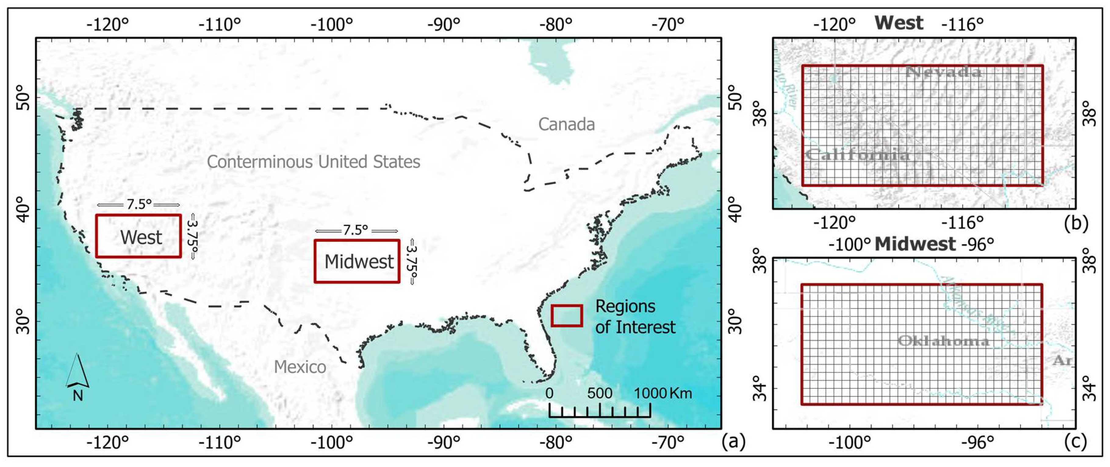
Our study was conducted over two regions of interest (ROI) within the conterminous United States (CONUS; Figure 1a). Each region encompasses a polygon of 7.5° × 3.75° (450 pixels with 30 columns and 15 rows in the native resolution of the ESA-CCI soil moisture product), and each ROI was aligned to the original edges of the ESA-CCI grid. Both areas were selected as they offer a contrast in climatic and topographic conditions, and anthropogenic activities such as different agricultural and forestry practices.
The West region (Figure 1b) comprises an area of 275,516 km2 with heterogeneous topographic features and a wide diversity of climate conditions ranging from the central valley of California in the West, passing through the densely forested areas in the Rocky Mountains, and water-limited ecosystems across California, Nevada, Utah, and Arizona.
The Midwest region (Figure 1c) comprises an area of 283,499 km2. This region lacks extensive mountainous areas (except for the Ouachita Mountains) and has a large influence of agricultural activity that strongly influences the dynamics of soil moisture. This region was also selected because of the extensive availability of ground-truth data [48] from the monitoring network MESONET [49], mainly over Oklahoma.
2.2. Input Data
2.2.1. Satellite-Derived Soil Moisture Data
We use information from the ESA-CCI soil moisture product Version 6.1 (revised in September 2021) which is the latest release by ESA-CCI [50]. ESA-CCI product merges daily data derived from C-band scatterometers (e.g., ERS-½, METOP) and data from multi-frequency radiometers (e.g., SMMR, SSM/I, TMI, AMSR-E, Windsat, AMSR-2, SMOS, SMAP, GPM, and FengYun-3B) at 0.25 degrees spatial resolution [51]. Based on daily soil moisture values, we calculated mean values for each pixel at the monthly and weekly scales for each ROI. Thus, obtaining 12 monthly layers and 52 weekly layers of mean soil moisture for the year 2010.
2.2.2. Terrain Parameters
Topographic information was derived from a digital elevation model (DEM) [52] and we extracted hydrologically meaningful terrain parameters for each ROI following a standardized approach [53]. Briefly, an initial set of 15 terrain parameters was calculated using the terrain analysis module in RSAGA [54], which implements SAGA GIS [55] in R statistical platform [56]. The original terrain parameters were: Aspect, Analytical Hillshading, Channel Network Base Level, Convergence Index, Cross Sectional Curvature, Catchment Area, Elevation, Flow Accumulation, Longitudinal Curvature, Length-Slope Factor, Relative Slope Position, Slope, Topographic Wetness Index, Valley Depth, and Vertical Distance to Channel Network. To reduce model complexity, identify the best prediction parameters, and avoid redundancy of information, we predicted soil moisture at 1 km over CONUS using different combinations of terrain parameters and geographic coordinates (i.e., latitude and longitude). This test was performed using a KKNN algorithm, combinations of the aforementioned predictors, and the ESA-CCI soil moisture annual mean of 2010 as the training dataset. Based on correlation and error values from cross-validation automatically performed during model training and evaluation, we identified the combination of predictors that best represented soil moisture reference values. Our results identified geographic coordinates (latitude and longitude) and 4 terrain parameters (elevation, aspect, slope, and topographic wetness index) as the best predictors for our study. Results of cross-validation from all the predictor combinations tested are included in Supplementary Material S1.
2.2.3. Data Used for Independent Validation
We validated downscaled soil moisture predictions using independent data from ground-truth soil moisture records from the North American Soil Moisture Database (NASMD). The NASMD integrates data from 33 observation networks, as well as 2 short-term monitoring campaigns that put together over 1800 observation sites across the United States, Canada, and Mexico [29]. We reiterate that data from the NASMD was not used for downscaling satellite-derived soil moisture, and only used for independent validation purposes.
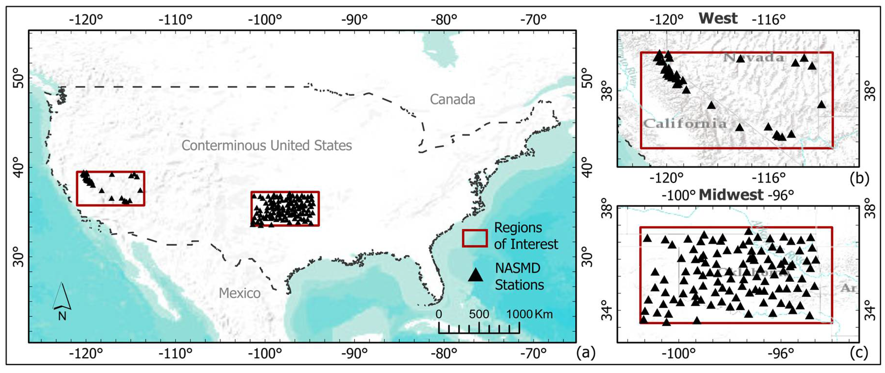
We selected all the available stations for the year 2010 with daily records of soil moisture in the top 5 cm of the soil layer for the two ROIs. The maximum number of available stations within CONUS was 743 (Figure 2a), while a maximum of 39 stations were available for the West region (Figure 2b) and a maximum of 116 were available for the Midwest region (Figure 2c). The number of stations available at the monthly and weekly scales ranged from ~26 to 39 in the West region, and from ~110 to 116 in the Midwest region (Supplementary Material S2). Monthly and weekly means of top 5 cm soil moisture records were calculated for each field station, to generate the reference data to validate monthly and weekly downscaled soil moisture predictions.
2.3. Data Preparation
2.3.1. Training Matrices
We generated a set of training matrices to obtain model parameters required by KKNN and RF. We selected the coordinates of the centroid of each original pixel (0.25 degrees) from the ESA-CCI product and assigned the soil moisture values to those coordinates. Then, we extracted the values of the 4 predefined terrain parameters at the finer resolution (1 km) that overlapped the ESA-CCI pixels centroids, and we added them to the training matrix. In each matrix, 70% of the available sampling points were randomly selected to conform the training dataset to build the models, and the 30% of remaining sampling points were set aside for further validation of models’ outputs.
Our final training matrices represent 12 monthly and 52 weekly files for each ROI, containing up to 315 records (70% of the maximum number of pixels available for each ROI that included soil moisture values and 6 predictors (4 terrain parameters, and latitude and longitude values)).
2.3.2. Prediction Matrices
We generated one matrix for each ROI to predict soil moisture at 1 km spatial resolution. We extracted all available records of the 4 predefined terrain parameters (predictors) at 1 km and added their corresponding coordinates to the prediction matrices. We integrated a total of 273,840 point locations into each of the two final prediction matrices; this number corresponds to the extension of the two ROIs in square kilometers, encompassing areas of 652 km (X-axis) by 420 km (Y-axis; Figure 1).
2.4. Downscaling Soil Moisture
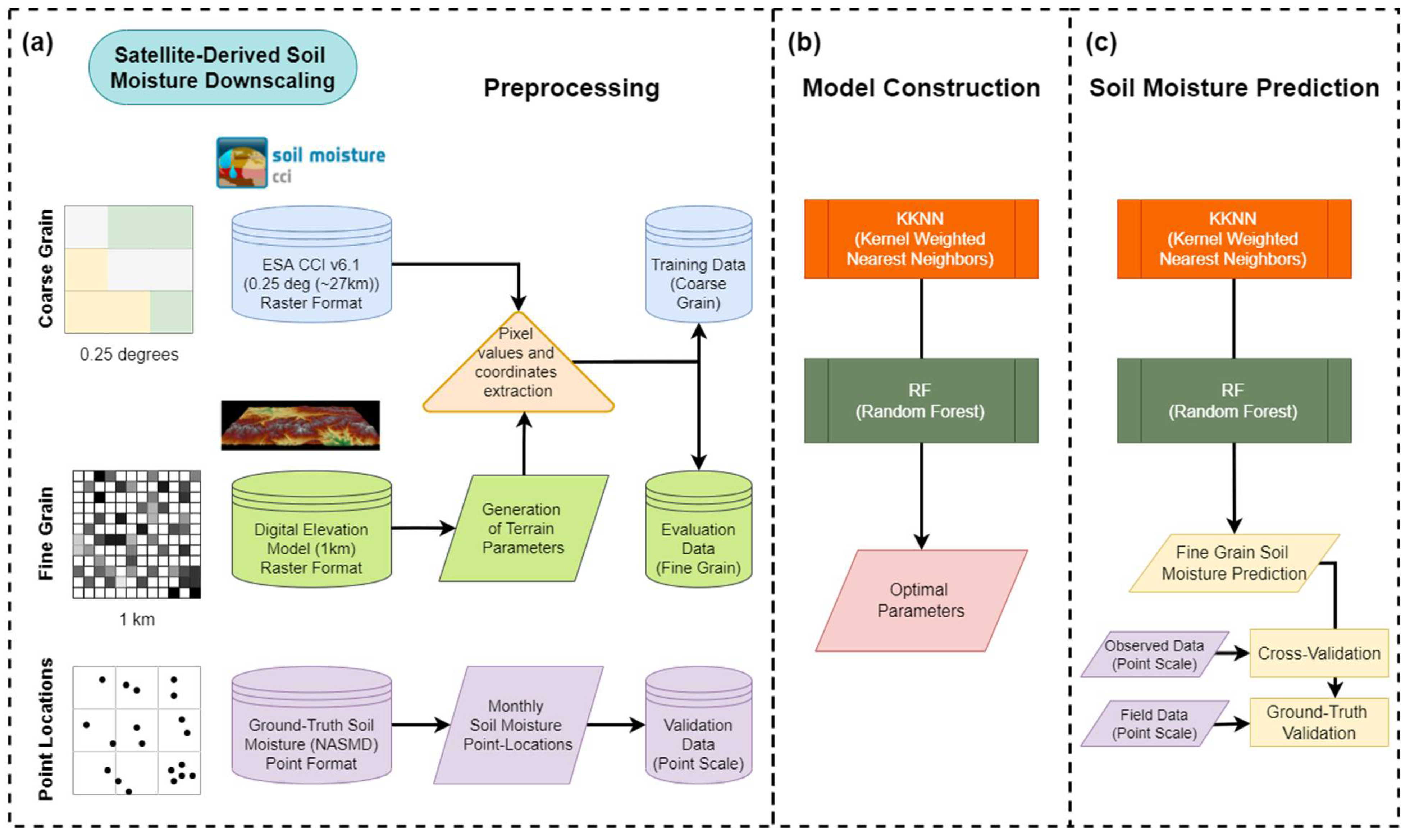
We used the modular framework of SOMOSPIE to predict soil moisture on a user-defined temporal (e.g., daily, monthly, annual) and spatial resolution (i.e., spatial granularity) to provide gap-free information within an ROI. The SOMOSPIE framework is composed of three main modules that include (1) preprocessing data from: satellite-derived soil moisture, predictive terrain parameters in the target resolution for downscaling (e.g., 1 km spatial resolution), and ground-truth reference data for independent validation purposes; (2) model construction: definition of optimal parameters for each modeling method (i.e., KKNN, RF); and (3) soil moisture prediction: application of model parameters defined in the previous module to predict soil moisture at the target resolution, as well as cross-validation and independent ground-truth validation (Figure 3).
We implemented our framework with two modeling methods (i.e., Kernel-Weighted K-Nearest Neighbors (KKNN) and Random Forest (RF)) to downscale soil moisture at 1 km over the two ROIs at monthly and weekly scales. We used the cloud-based cluster “Caviness” at the University of Delaware High Performance Computing (HPC) [57]. Caviness is a distributed-memory Linux cluster with 126 compute nodes representing 4536 cores with 24.6 TiB of RAM and 200 TB of storage.
2.4.1. Kernel-Weighted K-Nearest Neighbors (KKNN)
K-nearest neighbors (KKNN) in its traditional form is a regression technique that builds many simple models from local data [58], and is based upon decision rules that classify an unsampled point, based on the values of the nearest set of previously classified points or reference values in the sampling space [59]. This method assumes a different level of influence in the prediction space, where the nearest k-points to the target location are the ones with the most relevant influence, while the influence in the construction of the prediction model decreases with distance [45]. To assign distance-related relevance to predict soil moisture, a weighted mean of the k-nearest soil moisture ratios is calculated. This variant is based on the definition of kernel functions (i.e., Triangular, Epanechnikov, Gaussian, Optimal) that serve to find the number of neighbors (k) to be used in the prediction. The number of neighbors and the optimal kernel function are automatically selected through 10-fold cross validation [44,45].
The KKNN code used in the SOMOSPIE framework has been described previously [45] and has been successfully used to downscale satellite-derived soil moisture at different spatial scales [44]. The code is based on the ‘kknn’ package [60] developed for the R-statistical platform [56]. The definitions of optimal parameters found for each monthly and weekly layer in 2010, over the two ROIs, are shown in Supplementary Material S2.
2.4.2. Random Forest (RF)
Random Forest (RF) in the SOMOSPIE framework has been described previously [45] and is based on the ‘quantregForest’ package [61] developed for the R-statistical platform [56]. It is based on an ensemble of decision trees through a “bootstrap aggregation” process (bagging), which is a method to generate multiple versions of a predictor and then uses these versions to generate an aggregated predictor that depends on the values of a random vector independently sampled and weighed [62,63]. To predict values at an unsampled location, all decision trees in the ensemble are queried and their prediction outputs are combined through a weighted arithmetic mean. Techniques such as RF do not assume any particular geometric or functional form of the model and are suitable for sampling spaces with sparse data [45].
The definition of optimal parameters for soil moisture prediction with RF in SOMOSPIE considers two main values: (1) the number of trees to grow in the ensemble of regression trees and (2) the number of covariates randomly selected at each level of tree growth. The maximum number of trees allowed was 500, while the number of covariates changes in relation to the number of predictors defined as input (6 predictors for this study: latitude, longitude, elevation, aspect, slope, and topographic wetness index). The automatic variable selection is performed by ‘quantregForest’ through a cross-validation process. The optimal parameters selected for each monthly and weekly layer of 2010 over the two ROIs are reported in Supplementary Material S2.
2.5. Validation
To test the two modeling methods (i.e., KKNN and RF), we first used cross-validation with reference satellite-derived soil moisture data not used in the construction of the models, and then we used independent ground-truth soil moisture from the NASMD. We reiterate that the NASMD data was not used to parameterize any model and was only used for independent validation. Predicted soil moisture values were extracted from the 12 monthly and 52 weekly layers over the two ROIs, taking overlapping locations with the centroids of the ESA-CCI soil moisture reference data, and the point-locations of the NASMD available stations for each month and week, respectively.
2.5.1. Cross-Validation with Reference Satellite-Derived Soil Moisture Data
We calculated the correlation and root mean square error (RMSE) values based on matrices containing the predicted and reference values (from ESA-CCI data). The input data for this validation approach corresponds with the 30% of the sampling points set aside during the generation of the training matrices and were not used in the definition of the models’ parameters. The cross-validation data matrices contained up to 135 records, depending on the number of available reference points from the ESA-CCI mean values for each month and week.
The values of each predicted soil moisture pixel at a finer spatial resolution (i.e., 1 km) were compared with the reference values of satellite-derived soil moisture values at their original spatial resolution. The results from these analyses for each month and week over the two ROIs are reported in Supplementary Material S3.
2.5.2. Independent Validation with Ground-Truth Data
For these independent analyses, we calculated the overall correlation and RMSE between the predicted downscaled values from each method with the point-based ground-truth data from the NASMD. The results of correlation and RMSE between fine spatial resolution predicted soil moisture values and the point-based ground-truth data for each month and week over the two ROIs are reported in Supplementary Material S3.
2.5.3. Spatial Distribution of Prediction Outputs and Errors
To evaluate the performance of the two methods, we compared the mean values of all monthly and weekly predictions (12 monthly and 52 weekly outputs) in the two ROIs. We generated maps showing the mean values of ESA-CCI values at 0.25 degrees of spatial resolution and the mean values of our 1 km predictions over the set of 30% sampling points set aside for testing in each monthly and weekly scale. Thus, none of the points used in this approach to describe the spatial distribution of error were used to define the models’ parameters. We calculated the absolute difference between the mean of predicted soil moisture and the mean of ESA-CCI values at all our monthly and weekly scales over all the centroid coordinates of the ESA-CCI pixels. In a similar approach for all monthly and weekly scales, we calculated the absolute difference between the mean predicted soil moisture at 1 km and the mean values of the point-scale ground-truth records at the coordinates of all available NASMD stations during our time frame. Thus, we aim to observe the similarities in the spatial distribution between ESA-CCI data and the outputs of the two methods tested, as well as the distribution of the prediction errors.
3. Results
In this section, we present our 1 km soil moisture prediction results and evaluate the performance of the two methods used. We compared the predicted soil moisture values with the reference ESA-CCI values, and with independent values from the NASMD. The final soil moisture predictions at monthly and weekly scales over the two ROIs are available at the Consortium of Universities for the Advancement of Hydrologic Science data repository (HydroShare; doi:10.4211/hs.96eeb0d796a64b578f24e8154c166988) [64].
3.1. Optimal Model Parameters for Each Method
In the case of KKNN, we found that the automatic generation of model parameters defined a number of K-neighbors between 6 and 29 in the Midwest ROI for all models at monthly and weekly scales. Correlation ranged from 0.489 to 0.894, and RMSE from 0.03 to 0.046. In the West ROI, the number of K-neighbors ranged from 3 to 49, with correlation from 0.244 to 0.785, and RMSE from 0.025 to 0.055.
In the generation of RF models, we found that the number of covariates used as predictors in every model in the Midwest ROI ranged from two to six (out of six possible predefined predictors for this study). Correlation ranged from 0.537 to 0919, and RMSE from 0.028 to 0.043. In the West ROI, the number of covariates ranged from two to six. Correlation ranged from 0.413 to 0.833, and RMSE from 0.023 to 0.047.
All individual KKNN and RF models’ parameters are included in Supplementary Material S2.
3.2. Evaluation of Models’ Outputs
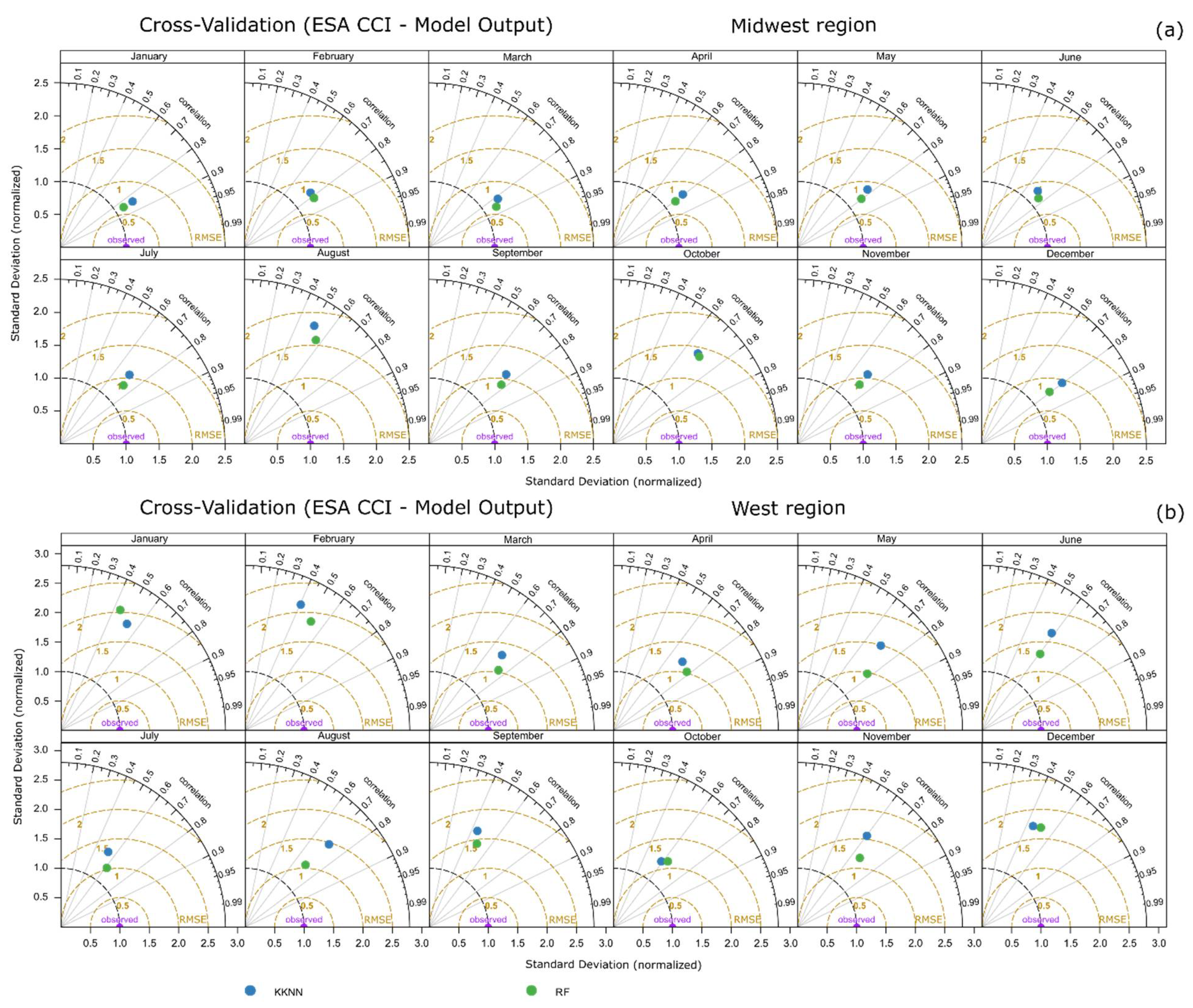
To evaluate the performance of each method tested, we present a series of Taylor Diagrams [65] that show the similarity of our predictions with both data from the ESA-CCI soil moisture values and independent ground-truth records from the NASMD. Taylor diagrams quantify the correspondence between reference observed data and predicted values by means of Pearson correlation coefficient, RMSE and the standard deviation.
3.2.1. Evaluation with Reference Satellite-Derived Soil Moisture Values
We found that RF was consistently the best method in predicting monthly soil moisture when compared against the reference values from the ESA-CCI values (Figure 4). RF correlation and RMSE values ranged from 0.566 to 0.856, and from 0.027 to 0.037, respectively, in the Midwest ROI. In the West ROI, RF correlation and RMSE values ranged from 0.443 to 0.78, and from 0.023 to 0.056, respectively. Regardless of the ROI, values predicted with RF showed the highest correlation and the lowest RMSE in every month, except in January in the West ROI.
Predictions with KKNN showed a consistent lower prediction performance than RF, with monthly correlation and RMSE values ranging from 0.508 to 0.844 and, 0.028 to 0.037, respectively, in the Midwest ROI. KKNN correlation and RMSE values in the West ROI ranged from 0.405 to 0.712 and from 0.023 to 0.054, respectively.
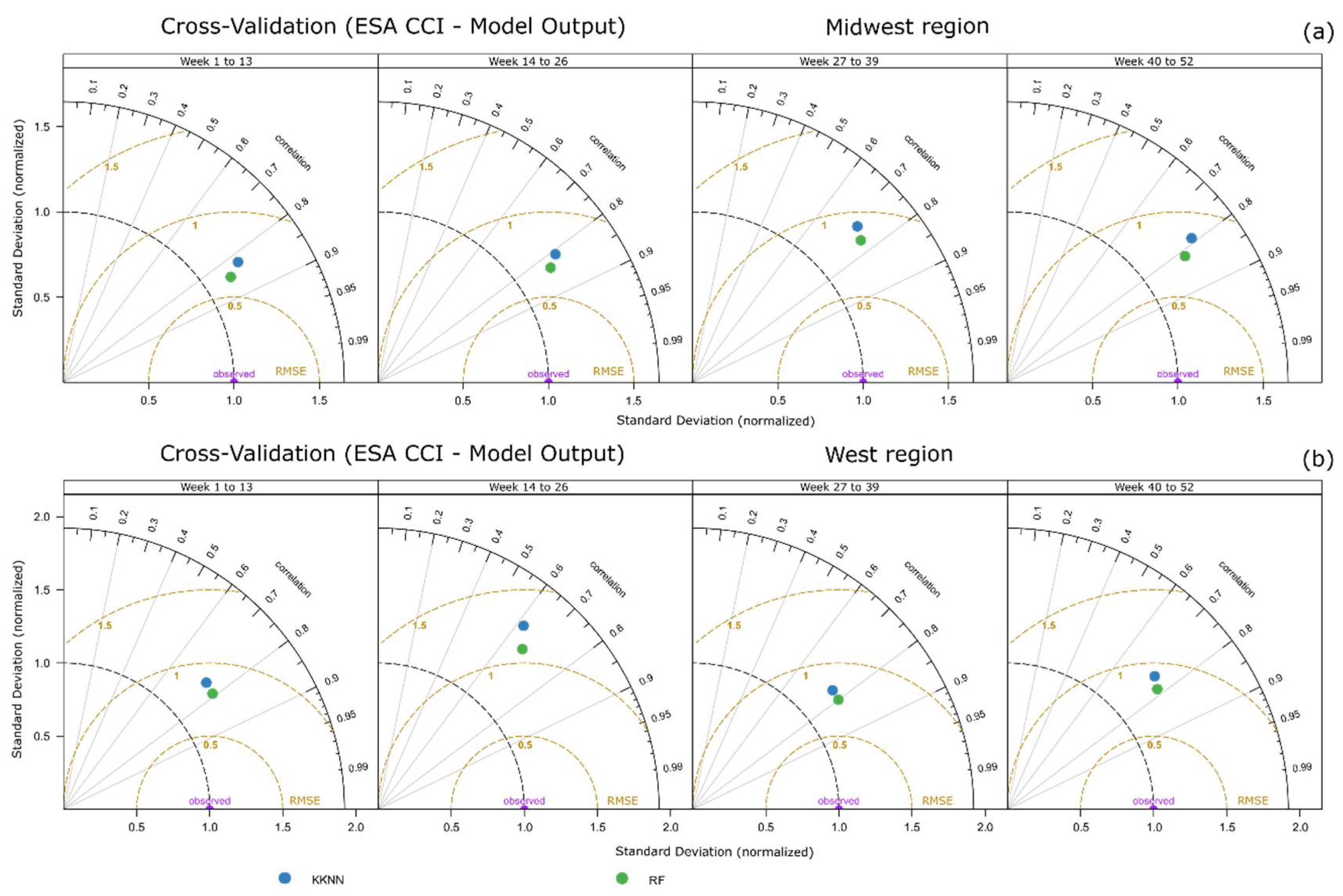
Similar to monthly predictions, we report the weekly performance of the two methods tested, grouping 52 weeks into four 3-month periods (Figure 5). Like monthly predictions, RF consistently showed better performance in all 3-month periods and in both ROIs. Correlation and RMSE values with RF ranged from 0.764 to 0.846, and 0.031 to 0.033, respectively, in the Midwest ROI, and from 0.634 to 0.785, and 0.026 to 0.041 in the West ROI. In contrast, correlation and RMSE values with KKNN in the Midwest region ranged from 0.726 to 0.823, and 0.033 to 0.036, while in the West ROI, these values ranged from 0.555 to 0.746, and 0.028 to 0.043, respectively.
All correlation and RMSE values shown in Figure 4 and Figure 5 are included in Supplementary Material S3.
3.2.2. Evaluation with Independent Ground-Truth Information
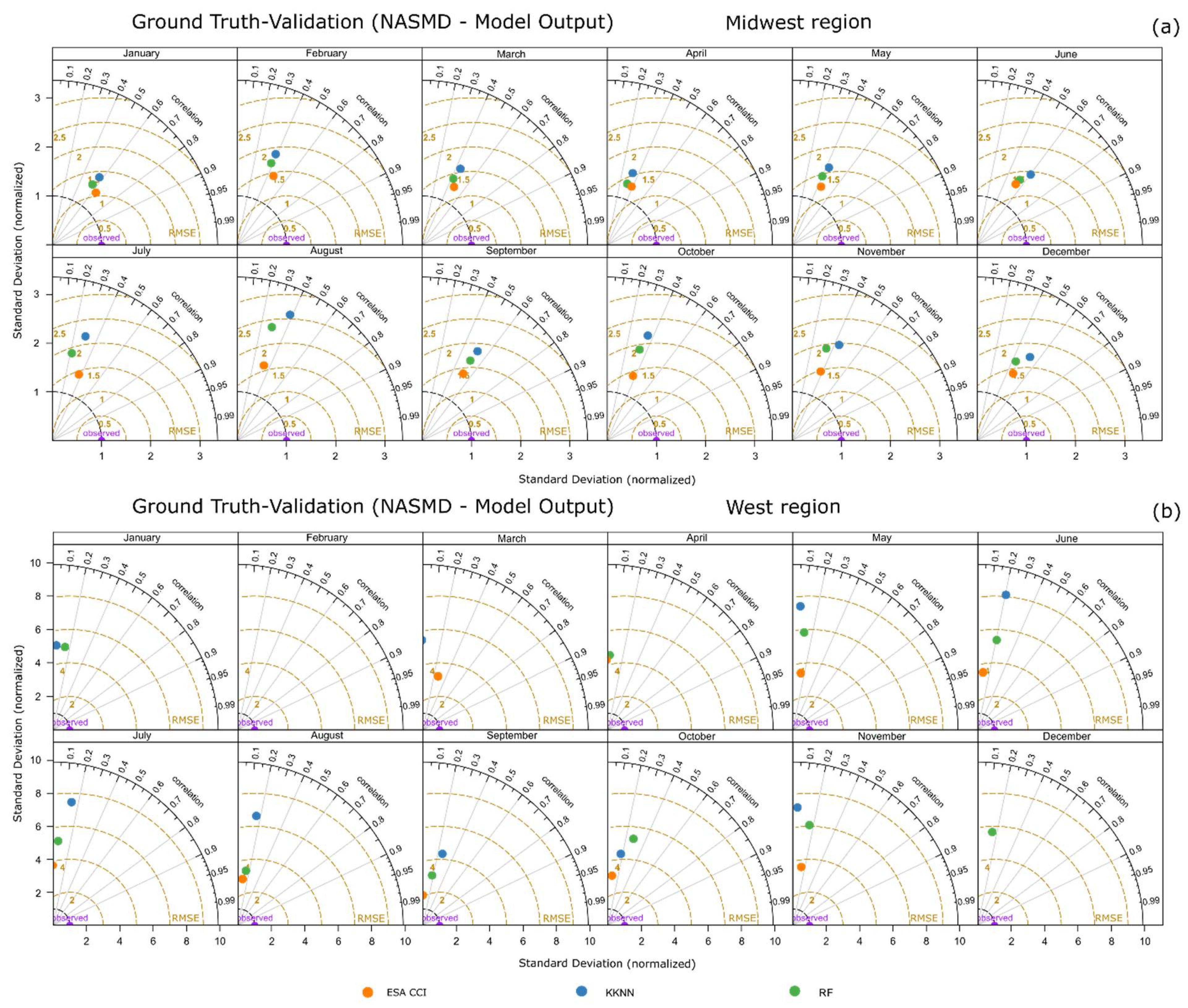
In Figure 6, we show the results of independent validation of monthly soil moisture predictions with ground-truth information from the NASMD. In the Midwest ROI, a similar correspondence between our predicted values and the reference data in all months was clear, except in August, where the ESA-CCI reference better corresponded with ground-truth records. Although the correlation and RMSE values for our two methods are consistently clustered in Figure 6a, RF showed a better correspondence with ground-truth data, and it was closer to the correlation and RMSE values of the reference satellite-derived values. A similar prediction performance was obtained for the West ROI (Figure 6b), where RF had consistently better agreement with the ground-truth reference data. However, the general agreement between ground-truth data, the reference satellite derived data and the models’ outputs was evidently lower in the West ROI.
The reference satellite-derived data monthly correlation and RMSE values with the ground-truth data ranged from 0.331 to 0.637 and 0.054 to 0.07 in the Midwest ROI, and from −0.953 to 0.272, and 0.078 to 0.167 in the West ROI, respectively. Monthly RF correlation and RMSE values in the Midwest ROI ranged from 0.216 to 0.55, and 0.052 to 0.073, while in the West ROI, these values ranged from −0.194 to 0.279, and 0.079 to 0.137, respectively. KKNN consistently showed the lowest correspondence with ground-truth data, except in October in the West ROI. KKNN correlation and RMSE values ranged from 0.3 to 0.603, and 0.051 to 0.069 in the Midwest ROI, and from −0.173 to 0.259, and 0.077 to 0.147 in the West ROI.
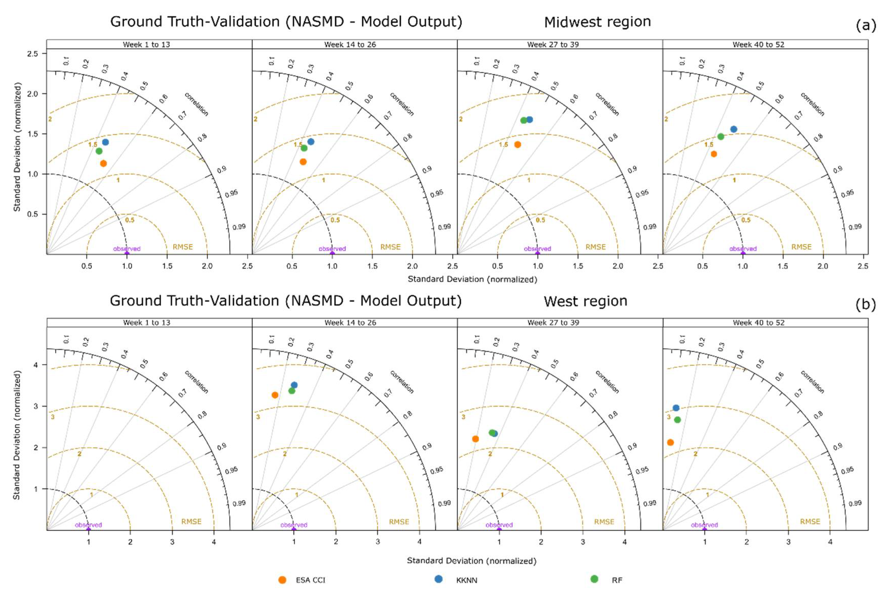
In the ground-truth validation of the weekly predictions (Figure 7), we found that the two methods showed similar correlation and RMSE values with ground truth data as the reference ESA-CCI in the Midwest ROI. Although there was not a clear pattern of better performance for either of the two methods tested, RF showed slightly better performance for the four 3-month periods in the Midwest ROI. In the West ROI, there was a consistent decrease in the correspondence between ground-truth data, our predictions, and the ESA-CCI values, although RF still showed a better performance in three of the four 3-month periods.
For weekly validation, ESA-CCI reference values exhibited the best correspondence with ground-truth data, with correlation and RMSE values ranging from 0.46 to 0.53, and 0.064 to 0.07 in the Midwest ROI, and from −0.195 to 0.166, and 0.097 to 0.132 in the West ROI. RF correlation and RMSE values ranged from 0.445, to 0.46, and 0.062 to 0.071 in the Midwest ROI, and from −0.041 to 0.158, and 0.091 to 0.126 in the West ROI. KKNN correlation and RMSE values, ranged from 0.464 to 0.494, and 0.06 to 0.069 in the Midwest ROI, and −0.077 to 0.154, and 0.09 to 0.126 in the West ROI.
All correlation and RMSE values shown in Figure 6 and Figure 7 are included in Supplementary Material S3.
3.3. Spatial Distribution of Prediction Errors
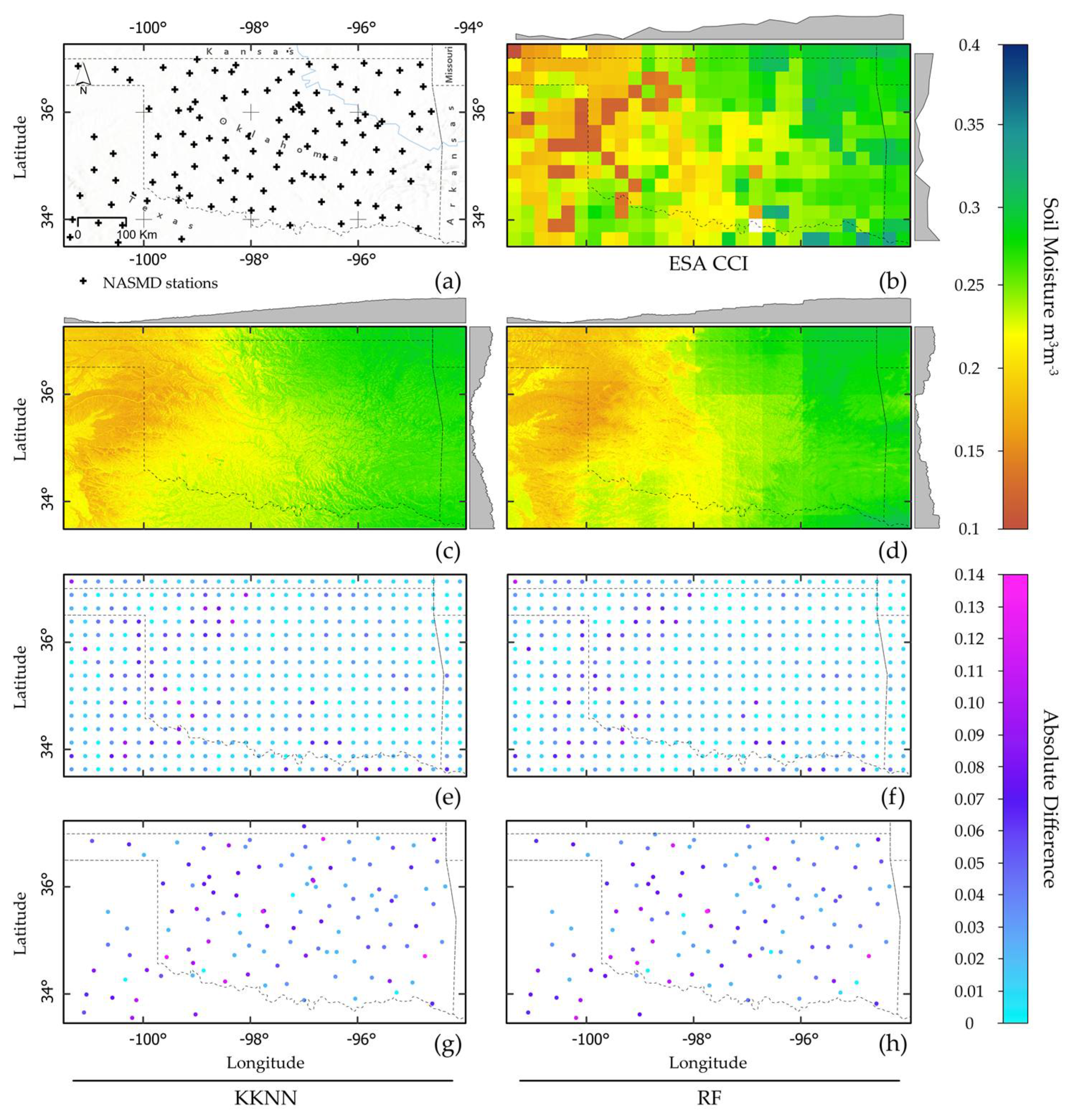
As we display in Figure 8c,d for the Midwest ROI, the spatial patterns of soil moisture values exhibited a similar behavior as the reference ESA-CCI values (Figure 8b). Similar to the ESA-CCI, the lowest soil moisture values were distributed over the west part of the ROI, and highest values over the east section. Low values were also consistent in the south-central portion, and high values in the central-north. The absolute differences between the 30% of sampling points set aside for testing in all layers derived from ESA-CCI values at 0.25 degrees and their spatially correspondent predicted soil moisture values in all layers at 1 km using the two methods tested are shown in Figure 8e,f. Difference values were distributed between 0 and 0.03 for both methods, with highest values in the western portion of the ROI. KKNN was the method with the lowest difference values over most of the ROI. In Figure 8g,h, we present the absolute differences between predicted soil moisture and ground-truth data. Difference values were constantly higher for the two methods in the Midwest ROI. Unlike the comparison between predicted soil moisture and reference ESA-CCI data, the performance of the two methods was similar when compared to ground-truth information. The lowest differences ranged between 0 and 0.04 m3 m−3, and the highest values were up to 0.14 m3 m−3. Although there was not a clear spatial distribution of the absolute differences, the distribution of low and high values was similar across the two methods.
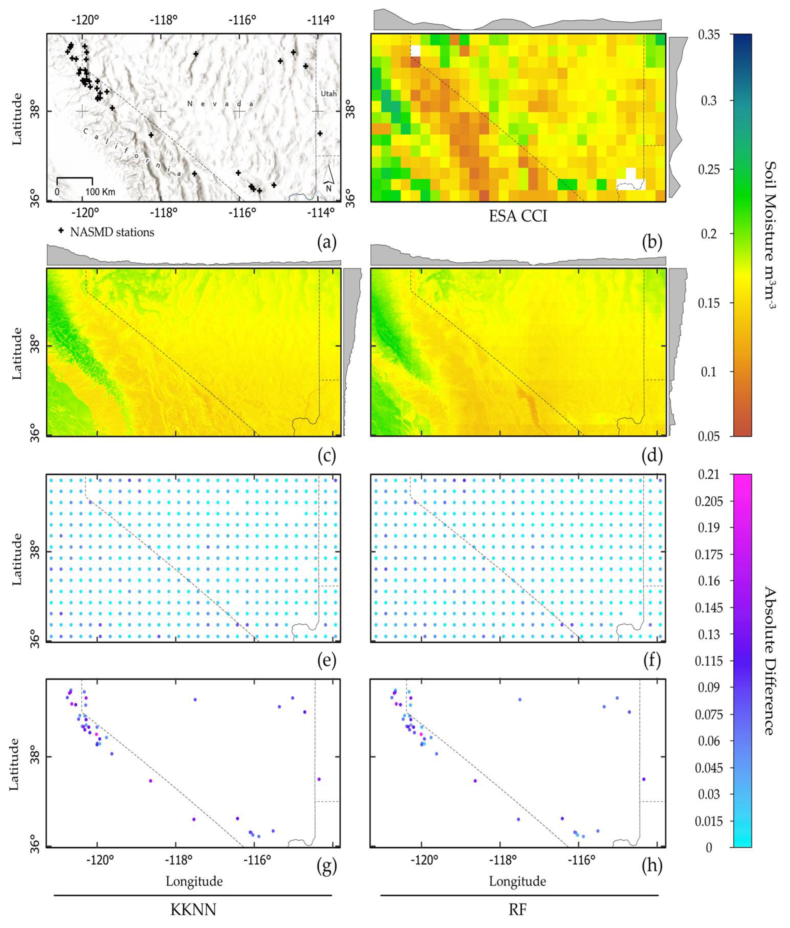
Figure 9 shows the spatial distribution of soil moisture predicted values and absolute differences with ESA-CCI values, and ground-truth data in the West ROI. Similar to ESA-CCI soil moisture, the lowest predicted values were distributed from the south-center to the north-west of the ROI (Figure 9c,d). However, low soil moisture values described a pattern not as dry as in the ESA-CCI data (between 0.05 and 0.1 m3 m−3). The highest predicted values with both methods were consistently located in two south-east to north-west lines, along the highest elevations of the Rocky Mountains and the central valley of California, ranging from 0.18 to 0.28 m3 m−3. Absolute differences between the 30% of test sampling points from ESA-CCI values at 0.25 degrees and their spatially correspondent prediction output values in all layers at 1 km in the West ROI can be observed in Figure 9e,f. Overall, the differences were consistently higher in the West ROI than in the Midwest ROI. The lowest difference values in the West ROI ranged between 0 and 0.045 m3 m−3, and highest values reached an absolute difference of 0.13 m3 m−3. Unlike the absolute differences shown in the Midwest ROI, in the West ROI, there was not a clear pattern in the spatial distribution of errors between ESCA-CCI and predicted values with our two methods. Absolute differences between predicted soil moisture and ground-truth data were consistently higher, regardless of the method used (Figure 9g,h). The distribution of the absolute differences across the locations with ground-truth data was similar for the two methods, although RF generally showed lower differences than KKNN. In contrast to the Midwest ROI, the absolute differences between predicted soil moisture and ground-truth information were significantly higher, ranging from 0.015 up to 0.21 m3 m−3.
4. Discussion
Our work shows the performance of two methods within the SOMOSPIE framework for downscaling satellite-derived soil moisture values. We used two ROIs with different topographic and climatic characteristics to compare the performance of the framework. Given the limitations in obtaining field-based measurements of soil moisture over large areas, flexible and adaptable frameworks are alternatives to obtain spatially and temporally detailed information. The SOMOSPIE framework offers an alternative approach to downscale satellite-derived soil moisture and to traditional predictions based on simple extrapolation and interpolation using information from monitoring networks [14,66,67].
Our framework demonstrates that it is possible to obtain soil moisture across different spatial and temporal scales, in relation to the resolution of the predictors and the temporal availability of the input satellite data. In our work, we used 1 km terrain parameters as predictors, but this framework could be extended to use topographic information at different spatial resolutions as input for further predictions. It is known that topography has different levels of influence on the spatial distribution of soil moisture [39], as previous studies have explored the impact of terrain characteristics at watershed and regional scales [40,42,44,45,68], and here, we showed that terrain parameters are suitable predictors at the regional scale. Although other environmental covariates, such as soil texture, surface temperature, and vegetation characteristics, are known to be correlated with the spatial and temporal distribution of soil moisture [3,39,40,69,70,71,72], these covariates did not offer significant advantages in our approach. First, soil texture is highly dependent on site-specific conditions [69] rather than our regional approach, while surface temperature and vegetation features might introduce bias that would hinder the effect of using solely terrain parameters as downscaling predictors [44].
We identified that latitude and longitude values, along with Aspect, Elevation, and Topographic Wetness Index, were the most suitable parameters to predict soil moisture at 1 km when using the two proposed methods. This aligns with previous studies that identified similar terrain parameters as relevant factors to derive soil moisture based on their relation with lateral distribution of water in the surface soil layer [40,43,73,74,75,76]. In general, we obtained better results with both algorithms in the Midwest ROI, where topographic characteristics are more homogenous than in the West ROI, with more complex terrain. Additionally, we saw similar patterns of soil moisture spatial distribution across coarse and fine scales, supporting previous work in downscaling satellite-derived soil moisture that found that spatial variability agrees with landscape heterogeneity [77]. We highlight that there is increasing evidence on how terrain parameters are useful for modeling soil moisture [39,74], but other environmental factors, such as precipitation, temperature, land cover, and soil properties [69,70,78], should be considered across different scenarios.
The SOMOSPIE framework takes advantage of daily values from the ESA-CCI soil moisture product, being able to predict soil moisture at different temporal scales (e.g., monthly, weekly). The comparison of predicted soil moisture across different periods helps to identify any temporal biases or patterns related to different environmental conditions throughout the year and identify emerging relationships with environmental factors at different points during wet-up and dry-down cycles [79,80]. In autumn and spring, topography becomes a more relevant indicator, whereas its importance decreases during summer and winter due to the influence of evapotranspiration, as well as extensive saturation and porosity control, respectively [74]. This might support the lower prediction performance observed during January and February in the West ROI, where topography plays a more important role in the spatial variability. Additionally, several studies have shown that more homogenous patterns of satellite-derived soil moisture occur under dry conditions, leading to an improved accuracy in satellite retrievals [81,82]. In this regard, the higher prediction accuracy we observed in the Midwest ROI might be linked to a lower retrieval error from ESA-CCI. This contrasts with the prediction accuracy in the West ROI, which might be impacted by a higher retrieval error of ESA-CCI, linked to more heterogeneous environmental conditions.
In general, we found that RF performed better at the monthly and weekly scales across both ROIs. This could be explained because this technique does not assume any particular geometric or functional form of the model. Furthermore, it is suitable in sampling spaces with sparse data [45], such as satellite-derived soil moisture in a coarse resolution, where the distance between pixels’ centroids yields substantial separation between data points. In contrast, although KKNN showed a lower prediction performance than RF, this technique still offers advantages for soil moisture downscaling in other regions with high density of sample points based on its ability to build many simple models when more data are available [59].
We observed that the two methods tested showed a similar correspondence to ground-truth information as the original ESA-CCI values in most of the monthly and weekly periods in our experiments. However, KKNN predictions showed a slightly better correspondence with ground-truth information in comparison with RF (values reporting the absolute correlation and RMSE differences between ground-truth information and ESA-CCI, as well as ground-truth and KKNN and RF outputs, are presented in Supplementary Materials S3). Differences in correlation and RMSE values between the two ROIs might be related to the sparse and uneven spatial distribution of available ground-truth stations in the West region (Figure 2). Previous studies found that the optimal number of ground-truth points for validating satellite-derived soil moisture products ranges from 10 to 20 per pixel [75], which is far from the desirable distribution of field stations available in the West ROI.
Although our work aimed at identifying the effect of terrain parameters in downscaling satellite-derived soil moisture information, other parameters, such as surface temperature, vegetation indexes, surface albedo, land cover, and rainfall, have been widely considered in previous research [3,39,40,71,72,75,83,84] and represent an opportunity to evaluate the flexibility of the SOMOSPIE framework.
5. Conclusions
Based on our analysis, we conclude that there is no “best” method that can be defined for every place in the world, as different methods perform differently in each ROI. As has been acknowledged in previous research, different downscaling methods have their own applicability under certain purposes, closely linked to differences in surface and climate conditions, and every method must be calibrated before its implementation elsewhere [39]. Thus, we believe that SOMOSPIE is a flexible framework that should include the methods tested in our work but is able to expand to incorporate additional methods to be tested in other regions around the world.
Despite the advantages of modeling techniques, such as KKNN and RF, in predicting soil moisture at a fine spatial resolution, it is also important to consider the computational resources needed when selecting these methods. When the ROI does not represent a large number of locations where soil moisture will be predicted, the two methods can be applied with no major challenges, but when the sampling space surpasses hundreds of thousands of locations, the selection of the modeling method and the use of computational resources become more important. The understanding of suitable cyberinfrastructure to work with more extensive regions and soil moisture predictions at finer spatial scales (e.g., 100 m, 30 m), along with the implementation of additional modeling methods in SOMOSPIE, is still being addressed through current efforts.
Our research contributes an alternative approach for downscaling satellite-derived soil moisture using a modular spatial inference framework. Here, we tested two methods, but the framework is flexible so multiple algorithms can be included [58,85]. Additional efforts to improve the SOMOSPIE framework include developing a containerized environment that will facilitate the deployment and management of the entire workflow in High-Performance Computing (HPC) or cloud environments [86].
Supplementary Materials
The following are available online at https://www.mdpi.com/article/10.3390/rs14133137/s1, Supplementary Materials S1: Selection of most relevant terrain parameters used as predictors to estimate soil moisture at 1 km spatial resolution over the conterminous United States. Refs. [44,45,52,54,55,56,57,58,59,60,87] are cited in the Supplementary Materials S1. Supplementary Materials S2: Number of North American Soil Moisture Database available stations in 2010 over the two regions of interest. Supplementary Materials S3: Cross-validation and ground-truth validation tables of monthly and weekly soil moisture predictions.
Author Contributions
R.M.L., L.V., M.T. and R.V. conceived and designed the research. R.M.L. and L.V. performed the experiments and analysis. R.M.L. wrote the first draft of the manuscript with input from L.V., P.O., M.T. and R.V.; R.M.L. wrote the code for data and analysis visualization and made the cartographic edition of map figures. P.O. contributed to the optimization of analyses performance in cloud-based computing environments. All authors contributed to interpretation of the results, reviewed, and approved the manuscript. R.V. and M.T. supervised and coordinated the research team and managed funding acquisition. All authors have read and agreed to the published version of the manuscript.
Funding
This study was funded by a University of Delaware Strategic Initiative research grant and the NSF (OAC grants #2103854 and #2103836 “Software Ecosystem for kNowledge diScOveRY-a data-driven framework for soil moisture applications”).
Data Availability Statement
Monthly and weekly soil moisture predictions at 1 km spatial resolution over the two regions of interested defined in this work can be accessed through HydroShare, https://doi.org/10.4211/hs.96eeb0d796a64b578f24e8154c166988 (accessed on 10 May 2022).
Acknowledgments
The authors want to acknowledge the support from the College of Agriculture and Natural Resources at the University of Delaware for supporting and facilitating research efforts among young scientists. We thank the UDIT Research Cyberinfrastructure unit for facilitating the analyses performed in this work through the Community Cluster Program. We are thankful for the valuable comments and contributions from current and former members of the Global computing Lab at the University of Tennessee, Knoxville: Danny Rorabaugh, Ria Patel, and Travis Johnston. RML and RV are thankful for the valuable comments and contributions from Mario Guevara.
Conflicts of Interest
The authors declare no conflict of interest.
References
- Ward, S. The Earth Observation Handbook—Climate Change Special Edition 2008; Bond, P., Ed.; Committee on Earth Observation Satellites, European Space Agency: Noordwijk, The Netherlands, 2008; ISBN 978-92-9221-408-1. [Google Scholar]
- Crow, W.T.; Wood, E.F. The Value of Coarse-Scale Soil Moisture Observations for Regional Surface Energy Balance Modeling. J. Hydrometeorol. 2002, 3, 467–482. [Google Scholar] [CrossRef] [Green Version]
- Legates, D.R.; Mahmood, R.; Levia, D.F.; DeLiberty, T.L.; Quiring, S.M.; Houser, C.; Nelson, F.E. Soil moisture: A central and unifying theme in physical geography. Prog. Phys. Geogr. 2010, 35, 65–86. [Google Scholar] [CrossRef]
- Williams, C.A.; Albertson, J.D. Soil moisture controls on canopy-scale water and carbon fluxes in an African savanna. Water Resour. Res. 2004, 40, 1–14. [Google Scholar] [CrossRef] [Green Version]
- Hamlet, A.F.; Mote, P.W.; Clark, M.P.; Lettenmaier, D.P. Twentieth-Century Trends in Runoff, Evapotranspiration, and Soil Moisture in the Western United States. J. Clim. 2007, 20, 1468–1486. [Google Scholar] [CrossRef] [Green Version]
- Narasimhan, B.; Srinivasan, R. Development and evaluation of Soil Moisture Deficit Index (SMDI) and Evapotranspiration Deficit Index (ETDI) for agricultural drought monitoring. Agric. For. Meteorol. 2005, 133, 69–88. [Google Scholar] [CrossRef]
- Davidson, E.A.; Belk, E.; Boone, R.D. Soil water content and temperature as independent or confounded factors controlling soil respiration in a temperate mixed hardwood forest. Glob. Chang. Biol. 1998, 4, 217–227. [Google Scholar] [CrossRef] [Green Version]
- Falloon, P.; Jones, C.D.; Ades, M.; Paul, K. Direct soil moisture controls of future global soil carbon changes: An important source of uncertainty. Glob. Biogeochem. Cycles 2011, 25, 1–14. [Google Scholar] [CrossRef] [Green Version]
- Vargas, R.; Allen, M.F. Environmental controls and the influence of vegetation type, fine roots and rhizomorphs on diel and seasonal variation in soil respiration. New Phytol. 2008, 179, 460–471. [Google Scholar] [CrossRef] [Green Version]
- Schaufler, G.; Kitzler, B.; Schindlbacher, A.; Skiba, U.; Sutton, M.A.; Zechmeister-Boltenstern, S. Greenhouse gas emissions from European soils under different land use: Effects of soil moisture and temperature. Eur. J. Soil Sci. 2010, 61, 683–696. [Google Scholar] [CrossRef]
- Vargas, R.; Baldocchi, D.D.; Allen, M.F.; Bahn, M.; Black, T.A.; Collins, S.L.; Yuste, J.C.; Hirano, T.; Jassal, R.S.; Pumpanen, J.; et al. Looking deeper into the soil: Biophysical controls and seasonal lags of soil CO2 production and efflux. Ecol. Appl. 2010, 20, 1569–1582. [Google Scholar] [CrossRef]
- Vargas, R.; Detto, M.; Baldocchi, D.D.; Allen, M.F. Multiscale analysis of temporal variability of soil CO2 production as influenced by weather and vegetation. Glob. Chang. Biol. 2010, 16, 1589–1605. [Google Scholar] [CrossRef]
- Baldocchi, D. “Breathing” of the terrestrial biosphere: Lessons learned from a global network of carbon dioxide flux measurement systems. Aust. J. Bot. 2008, 56, 1–26. [Google Scholar] [CrossRef]
- Chen, H.; Fan, L.; Wu, W.; Liu, H.-B. Comparison of spatial interpolation methods for soil moisture and its application for monitoring drought. Environ. Monit. Assess. 2017, 189, 525. [Google Scholar] [CrossRef] [PubMed]
- Dorigo, W.; Wagner, W.; Albergel, C.; Albrecht, F.; Balsamo, G.; Brocca, L.; Chung, D.; Ertl, M.; Forkel, M.; Gruber, A.; et al. ESA CCI Soil Moisture for improved Earth system understanding: State-of-the art and future directions. Remote Sens. Environ. 2017, 203, 185–215. [Google Scholar] [CrossRef]
- Martínez-Fernández, J.; González-Zamora, A.; Sánchez, N.; Gumuzzio, A.; Herrero-Jiménez, C.M. Satellite soil moisture for agricultural drought monitoring: Assessment of the SMOS derived Soil Water Deficit Index. Remote Sens. Environ. 2016, 177, 277–286. [Google Scholar] [CrossRef]
- Crow, W.T. Utility of soil moisture data products for natural disaster applications. In Extreme Hydroclimatic Events and Multivariate Hazards in a Changing Environment; Maggioni, V., Nassari, C., Eds.; Elsevier: San Diego, CA, USA, 2019; pp. 65–85. [Google Scholar]
- Engman, E.T. Applications of microwave remote sensing of soil moisture for water resources and agriculture. Remote Sens. Environ. 1991, 35, 213–226. [Google Scholar] [CrossRef]
- Kimmins, J.P. From science to stewardship: Harnessing forest ecology in the service of society. For. Ecol. Manag. 2008, 256, 1625–1635. [Google Scholar] [CrossRef]
- Koster, R.D.; Suarez, M.J. Soil Moisture Memory in Climate Models. J. Hydrometeorol. 2001, 2, 558–570. [Google Scholar] [CrossRef]
- Meehl, G.A.; Washington, W.M. A Comparison of Soil-Moisture Sensitivity in Two Global Climate Models. J. Atmos. Sci. 1988, 45, 1476–1492. [Google Scholar] [CrossRef] [Green Version]
- Seneviratne, S.I.; Corti, T.; Davin, E.L.; Hirschi, M.; Jaeger, E.B.; Lehner, I.; Orlowsky, B.; Teuling, A.J. Investigating soil moisture-climate interactions in a changing climate: A review. Earth-Sci. Rev. 2010, 99, 125–161. [Google Scholar] [CrossRef]
- Walker, J.P.; Willgoose, G.R.; Kalma, J.D. In situ measurement of soil moisture: A comparison of techniques. J. Hydrol. 2004, 293, 85–99. [Google Scholar] [CrossRef]
- Martínez-Fernández, J.; Ceballos, A. Temporal Stability of Soil Moisture in a Large-Field Experiment in Spain. Soil Sci. Soc. Am. J. 2003, 67, 1647–1656. [Google Scholar] [CrossRef]
- Robock, A.; Mu, M.; Vinnikov, K.; Trofimova, I.V.; Adamenko, T.I. Forty-five years of observed soil moisture in the Ukraine: No summer desiccation (yet). Geophys. Res. Lett. 2005, 32, L03401. [Google Scholar] [CrossRef] [Green Version]
- Dorigo, W.A.; Xaver, A.; Vreugdenhil, M.; Gruber, A.; Hegyiová, A.; Sanchis-Dufau, A.D.; Zamojski, D.; Cordes, C.; Wagner, W.; Drusch, M. Global Automated Quality Control of In Situ Soil Moisture Data from the International Soil Moisture Network. Vadose Zone J. 2013, 12, 1–21. [Google Scholar] [CrossRef]
- Dorigo, W.A.; Wagner, W.; Hohensinn, R.; Hahn, S.; Paulik, C.; Xaver, A.; Gruber, A.; Drusch, M.; Mecklenburg, S.; van Oevelen, P.; et al. The International Soil Moisture Network: A data hosting facility for global in situ soil moisture measurements. Hydrol. Earth Syst. Sci. 2011, 15, 1675–1698. [Google Scholar] [CrossRef] [Green Version]
- Schaefer, G.L.; Cosh, M.H.; Jackson, T.J. The USDA Natural Resources Conservation Service Soil Climate Analysis Network (SCAN). J. Atmos. Ocean. Technol. 2007, 24, 2073–2077. [Google Scholar] [CrossRef]
- Quiring, S.M.; Ford, T.W.; Wang, J.K.; Khong, A.; Harris, E.; Lindgren, T.; Goldberg, D.W.; Li, Z. The North American Soil Moisture Database: Development and Applications. Bull. Am. Meteorol. Soc. 2016, 97, 1441–1459. [Google Scholar] [CrossRef]
- Entekhabi, D.; Njoku, E.G.; O’Neill, P.E.; Kellogg, K.H.; Crow, W.T.; Edelstein, W.N.; Entin, J.K.; Goodman, S.D.; Jackson, T.J.; Johnson, J.; et al. The Soil Moisture Active Passive (SMAP) Mission. Proc. IEEE 2010, 98, 704–716. [Google Scholar] [CrossRef]
- Das, N.N.; Entekhabi, D.; Dunbar, R.S.; Colliander, A.; Chen, F.; Crow, W.; Jackson, T.J.; Berg, A.; Bosch, D.D.; Caldwell, T.; et al. The SMAP mission combined active-passive soil moisture product at 9 km and 3 km spatial resolutions. Remote Sens. Environ. 2018, 211, 204–217. [Google Scholar] [CrossRef]
- Liu, Y.Y.; Parinussa, R.M.; Dorigo, W.A.; De Jeu, R.A.M.; Wagner, W.; van Dijk, A.I.J.M.; McCabe, M.F.; Evans, J.P. Developing an improved soil moisture dataset by blending passive and active microwave satellite-based retrievals. Hydrol. Earth Syst. Sci. 2011, 15, 425–436. [Google Scholar] [CrossRef] [Green Version]
- Peng, J.; Loew, A. Recent Advances in Soil Moisture Estimation from Remote Sensing. Water 2017, 9, 530. [Google Scholar] [CrossRef] [Green Version]
- Mohanty, B.P.; Cosh, M.H.; Lakshmi, V.; Montzka, C. Soil Moisture Remote Sensing: State-of-the-Science. Vadose Zone J. 2017, 16, 1–9. [Google Scholar] [CrossRef] [Green Version]
- Barre, H.M.J.P.; Duesmann, B.; Kerr, Y.H. SMOS: The Mission and the System. IEEE Trans. Geosci. Remote Sens. 2008, 46, 587–593. [Google Scholar] [CrossRef]
- Paloscia, S.; Pettinato, S.; Santi, E.; Notarnicola, C.; Pasolli, L.; Reppucci, A. Soil moisture mapping using Sentinel-1 images: Algorithm and preliminary validation. Remote Sens. Environ. 2013, 134, 234–248. [Google Scholar] [CrossRef]
- Srivastava, P.K.; Pandey, P.C.; Petropoulos, G.P.; Kourgialas, N.N.; Pandey, V.; Singh, U. GIS and Remote Sensing Aided Information for Soil Moisture Estimation: A Comparative Study of Interpolation Techniques. Resources 2019, 8, 70. [Google Scholar] [CrossRef] [Green Version]
- Dorigo, W.A.; Gruber, A.; De Jeu, R.A.M.; Wagner, W.; Stacke, T.; Loew, A.; Albergel, C.; Brocca, L.; Chung, D.; Parinussa, R.M.; et al. Evaluation of the ESA CCI soil moisture product using ground-based observations. Remote Sens. Environ. 2015, 162, 380–395. [Google Scholar] [CrossRef]
- Peng, J.; Loew, A.; Merlin, O.; Verhoest, N.E.C. A review of spatial downscaling of satellite remotely sensed soil moisture. Rev. Geophys. 2017, 55, 341–366. [Google Scholar] [CrossRef]
- Busch, F.A.; Niemann, J.D.; Coleman, M. Evaluation of an empirical orthogonal function-based method to downscale soil moisture patterns based on topographical attributes. Hydrol. Process. 2012, 26, 2696–2709. [Google Scholar] [CrossRef]
- Ranney, K.J.; Niemann, J.D.; Lehman, B.M.; Green, T.R.; Jones, A.S. A method to downscale soil moisture to fine resolutions using topographic, vegetation, and soil data. Adv. Water Resour. 2015, 76, 81–96. [Google Scholar] [CrossRef] [Green Version]
- Coleman, M.L.; Niemann, J.D. Controls on topographic dependence and temporal instability in catchment-scale soil moisture patterns. Water Resour. Res. 2013, 49, 1625–1642. [Google Scholar] [CrossRef]
- Droesen, J.M. Downscaling Soil Moisture Using Topography—The Evaluation and Optimisation of a Downscaling Approach. Master’s Thesis, Wageningen University, Wageningen, The Netherlands, 2016. [Google Scholar]
- Guevara, M.; Vargas, R. Downscaling satellite soil moisture using geomorphometry and machine learning. PLoS ONE 2019, 14, e0219639. [Google Scholar] [CrossRef] [PubMed] [Green Version]
- Rorabaugh, D.; Guevara, M.; Llamas, R.; Kitson, J.; Vargas, R.; Taufer, M. SOMOSPIE: A Modular SOil MOisture SPatial Inference Engine Based on Data-Driven Decisions. In Proceedings of the 2019 15th International Conference on eScience (eScience), IEEE, San Diego, CA, USA, 24–27 September 2019; pp. 1–10. [Google Scholar] [CrossRef] [Green Version]
- Kitson, T.; Olaya, P.; Racca, E.; Wyatt, M.R.; Guevara, M.; Vargas, R.; Taufer, M. Data analytics for modeling soil moisture patterns across united states ecoclimatic domains. In Proceedings of the 2017 IEEE International Conference on Big Data (Big Data), Boston, MA, USA, 11–14 December 2017; pp. 4768–4770. [Google Scholar]
- McKinney, R.; Pallipuram, V.K.; Vargas, R.; Taufer, M. From HPC Performance to Climate Modeling: Transforming Methods for HPC Predictions into Models of Extreme Climate Conditions. In Proceedings of the 2015 IEEE 11th International Conference on e-Science, Munich, Germany, 31 August–4 September 2015; pp. 108–117. [Google Scholar]
- Llamas, R.M.; Guevara, M.; Rorabaugh, D.; Taufer, M.; Vargas, R. Spatial Gap-Filling of ESA CCI Satellite-Derived Soil Moisture Based on Geostatistical Techniques and Multiple Regression. Remote Sens. 2020, 12, 665. [Google Scholar] [CrossRef] [Green Version]
- Brock, F.V.; Crawford, K.C.; Elliott, R.L.; Cuperus, G.W.; Stadler, S.J.; Johnson, H.L.; Eilts, M.D. The Oklahoma Mesonet: A Technical Overview. J. Atmos. Ocean. Technol. 1995, 12, 5–19. [Google Scholar] [CrossRef]
- Hirschi, M.; Nicolai-Shaw, N.; Preimesberger, W.; Scanlon, T.; Dorigo, W.; Kidd, R. Product Validation and Intercomparison Report (PVIR), Supporting Product, version v06.1; European Space Agency: Vienna, Austria, 2021. [Google Scholar]
- van der Schalie, R.; Preimesberger, W.; Pasik, A.; Scanlon, T.; Kidd, R. ESA Climate Change Initiative Plus Soil Moisture, Product User Guide, Supporting Product, version v06.1; European Space Agency: Vienna, Austria, 2021. [Google Scholar]
- Becker, J.J.; Sandwell, D.T.; Smith, W.H.F.; Braud, J.; Binder, B.; Depner, J.; Fabre, D.; Factor, J.; Ingalls, S.; Kim, S.-H.; et al. Global Bathymetry and Elevation Data at 30 Arc Seconds Resolution: SRTM30_PLUS. Mar. Geod. 2009, 32, 355–371. [Google Scholar] [CrossRef]
- Guevara, M.; Vargas, R. Annual Soil Moisture Predictions across Conterminous United States Using Remote Sensing and Terrain Analysis across 1 km Grids (1991–2016). 2019. Available online: https://doi.org/10.4211/hs.b8f6eae9d89241cf8b5904033460af61 (accessed on 17 February 2022).
- Brenning, A.; Bangs, D.; Becker, M. RSAGA: SAGA Geoprocessing and Terrain Analysis in R (1.3.0). 2008. Available online: https://github.com/r-spatial/RSAGA (accessed on 23 July 2021).
- Conrad, O.; Bechtel, B.; Bock, M.; Dietrich, H.; Fischer, E.; Gerlitz, L.; Wehberg, J.; Wichmann, V.; Böhner, J. System for Automated Geoscientific Analyses (SAGA) v. 2.1.4. Geosci. Model Dev. 2015, 8, 1991–2007. [Google Scholar] [CrossRef] [Green Version]
- R Core Team. R: A Language and Environment for Statistical Computing (4.0.3); R Foundation for Statistical Computing: Vienna, Austria, 2020; Available online: https://www.r-project.org/ (accessed on 27 August 2021).
- UDIT Research CyberInfrastructure CAVINESS, Supporting Researchers at University of Delaware. Available online: https://sites.udel.edu/it-rci/compute/community-cluster-program/caviness/ (accessed on 23 August 2021).
- Johnston, T.; Zanin, C.; Taufer, M. HYPPO: A Hybrid, Piecewise Polynomial Modeling Technique for Non-Smooth Surfaces. In Proceedings of the 2016 28th International Symposium on Computer Architecture and High Performance Computing (SBAC-PAD), Los Angeles, CA, USA, 26–28 October 2016; pp. 26–33. [Google Scholar] [CrossRef]
- Cover, T.; Hart, P. Nearest neighbor pattern classification. IEEE Trans. Inf. Theory 1967, 13, 21–27. [Google Scholar] [CrossRef] [Green Version]
- Hechenbichler, K.; Schliep, K. Weighted k-Nearest-Neighbor Techniques and Ordinal Classification; Collaborative Research Center 386, Discussion Paper 399; Ludwig-Maximilians-Universität München: Munich, Germany, 2004. [Google Scholar] [CrossRef]
- Meinshausen, N. Quantile Regression Forests. J. Mach. Learn. Res. 2006, 7, 983–999. [Google Scholar]
- Breiman, L. Bagging Predictors. Mach. Learn. 1996, 24, 123–140. [Google Scholar] [CrossRef] [Green Version]
- Breiman, L. Random forests. Mach. Learn. 2001, 45, 5–32. [Google Scholar] [CrossRef] [Green Version]
- Llamas, R.M.; Valera, L.; Olaya, P.; Taufer, M.; Vargas, R. 1-km Soil Moisture Predictions in the United States with SOMOSPIE Framework. 2022. Available online: https://doi.org/10.4211/hs.96eeb0d796a64b578f24e8154c166988 (accessed on 10 May 2022).
- Taylor, K.E. Summarizing multiple aspects of model performance in a single diagram. J. Geophys. Res. 2001, 106, 7183–7192. [Google Scholar] [CrossRef]
- Bárdossy, A.; Lehmann, W. Spatial distribution of soil moisture in a small catchment. Part 1: Geostatistical analysis. J. Hydrol. 1998, 206, 1–15. [Google Scholar] [CrossRef]
- Ding, Y.; Wang, Y.; Miao, Q. Research on the spatial interpolation methods of soil moisture based on GIS. In Proceedings of the International Conference on Information Science and Technology, ICIST 2011, Nanjing, China, 26–28 March 2011; pp. 709–711. [Google Scholar] [CrossRef]
- Escorihuela, M.J.; Quintana-Seguí, P. Comparison of remote sensing and simulated soil moisture datasets in Mediterranean landscapes. Remote Sens. Environ. 2016, 180, 99–114. [Google Scholar] [CrossRef] [Green Version]
- Loew, A.; Mauser, W. On the Disaggregation of Passive Microwave Soil Moisture Data using a Priori Knowledge of Temporally Persistent Soil Moisture Fields. In Proceedings of the IGARSS 2008—2008 IEEE International Geoscience and Remote Sensing Symposium, Boston, MA, USA, 7–11 July 2008; Volume 3, pp. III-226–III-229. [Google Scholar]
- Mattikalli, N.M.; Engman, E.T.; Jackson, T.J.; Ahuja, L.R. Microwave remote sensing of temporal variations of brightness temperature and near-surface soil water content during a watershed-scale field experiment, and its application to the estimation of soil physical properties. Water Resour. Res. 1998, 34, 2289–2299. [Google Scholar] [CrossRef]
- Merlin, O.; Chehbouni, A.; Kerr, Y.H.; Goodrich, D.C. A downscaling method for distributing surface soil moisture within a microwave pixel: Application to the Monsoon ’90 data. Remote Sens. Environ. 2006, 101, 379–389. [Google Scholar] [CrossRef]
- Kovačević, J.; Cvijetinović, Ž.; Stančić, N.; Brodić, N.; Mihajlović, D. New downscaling approach using ESA CCI SM products for obtaining high resolution surface soil moisture. Remote Sens. 2020, 12, 1119. [Google Scholar] [CrossRef] [Green Version]
- Western, A.W.; Blöschl, G. On the spatial scaling of soil moisture. J. Hydrol. 1999, 217, 203–224. [Google Scholar] [CrossRef]
- Western, A.W.; Grayson, R.B.; Blöschl, G.; Willgoose, G.R.; McMahon, T.A. Observed spatial organization of soil moisture and its relation to terrain indices. Water Resour. Res. 1999, 35, 797–810. [Google Scholar] [CrossRef] [Green Version]
- Crow, W.T.; Berg, A.A.; Cosh, M.H.; Loew, A.; Mohanty, B.P.; Panciera, R.; de Rosnay, P.; Ryu, D.; Walker, J.P. Upscaling sparse ground-based soil moisture observations for the validation of coarse-resolution satellite soil moisture products. Rev. Geophys. 2012, 50, 1–20. [Google Scholar] [CrossRef] [Green Version]
- Julien, P.Y.; Moglen, G.E. Similarity and length scale for spatially varied overland flow. Water Resour. Res. 1990, 26, 1819–1832. [Google Scholar] [CrossRef]
- van der Velde, R.; Salama, M.S.; Eweys, O.A.; Wen, J.; Wang, Q. Soil Moisture Mapping Using Combined Active/Passive Microwave Observations Over the East of the Netherlands. IEEE J. Sel. Top. Appl. Earth Obs. Remote Sens. 2015, 8, 4355–4372. [Google Scholar] [CrossRef]
- Kim, G.; Chung, J.; Kim, J. Spatial characterization of soil moisture estimates from the Southern Great Plain (SGP 97) hydrology experiment. KSCE J. Civ. Eng. 2002, 6, 177–184. [Google Scholar] [CrossRef]
- Panciera, R. Effect of Land Surface Heterogeneity on Satellite Near-Surface Soil Moisture Observations. Ph.D. Thesis, University of Melbourne, Melbourne, Australia, 2009. [Google Scholar]
- Vachaud, G.; Passerat De Silans, A.; Balabanis, P.; Vauclin, M. Temporal Stability of Spatially Measured Soil Water Probability Density Function. Soil Sci. Soc. Am. J. 1985, 49, 822–828. [Google Scholar] [CrossRef]
- Wigneron, J.-P.; Waldteufel, P.; Chanzy, A.; Calvet, J.-C.; Kerr, Y. Two-Dimensional Microwave Interferometer Retrieval Capabilities over Land Surfaces (SMOS Mission). Remote Sens. Environ. 2000, 73, 270–282. [Google Scholar] [CrossRef]
- Friesen, J.; Rodgers, C.; Ogunrunde, P.G.; Hendrickx, J.M.H.; Van De Giesen, N. Hydrotope-based protocol to determine average soil moisture over large areas for satellite calibration and validation with results from an observation campaign in the Volta Basin, West Africa. IEEE Trans. Geosci. Remote Sens. 2008, 46, 1995–2004. [Google Scholar] [CrossRef] [Green Version]
- Kim, G.; Barros, A. Downscaling of remotely sensed soil moisture with a modified fractal interpolation method using contraction mapping and ancillary data. Remote Sens. Environ. 2002, 83, 400–413. [Google Scholar] [CrossRef]
- Temimi, M.; Leconte, R.; Chaouch, N.; Sukumal, P.; Khanbilvardi, R.; Brissette, F. A combination of remote sensing data and topographic attributes for the spatial and temporal monitoring of soil wetness. J. Hydrol. 2010, 388, 28–40. [Google Scholar] [CrossRef]
- Johnston, T.; Alsulmi, M.; Cicotti, P.; Taufer, M. Performance tuning of MapReduce jobs using surrogate-based modeling. Procedia Comput. Sci. 2015, 51, 49–59. [Google Scholar] [CrossRef] [Green Version]
- Olaya, P.; Kennedy, D.; Llamas, R.; Valera, L.; Vargas, R.; Lofstead, J.; Taufer, M. Building Trust in Earth Science Findings through Data Traceability and Results Explainability. Trans. Parallel Distrib. Syst. 2022. submitted. [Google Scholar]
- Hallema, D.W.; Moussa, R.; Sun, G.; Mcnulty, S.G. Surface storm flow prediction on hillslopes based on topography and hydrologic connectivity. Ecol. Process. 2016, 5, 13. [Google Scholar] [CrossRef] [Green Version]
Figure 1.
(a) Regions of interest (ROIs) for soil moisture downscaling; (b) West ROI; (c) Midwest ROI.
Figure 1.
(a) Regions of interest (ROIs) for soil moisture downscaling; (b) West ROI; (c) Midwest ROI.

Figure 2.
(a) North American Soil Moisture Database (NASMD) stations over the two ROIs available in 2010; (b) West ROI; and (c) Midwest ROI.
Figure 2.
(a) North American Soil Moisture Database (NASMD) stations over the two ROIs available in 2010; (b) West ROI; and (c) Midwest ROI.

Figure 3.
Framework for soil moisture prediction at 1 km spatial resolution derived from coarse resolution ESA-CCI values; (a) data preprocessing; (b) model construction; (c) soil moisture prediction and validation.
Figure 3.
Framework for soil moisture prediction at 1 km spatial resolution derived from coarse resolution ESA-CCI values; (a) data preprocessing; (b) model construction; (c) soil moisture prediction and validation.

Figure 4.
Taylor diagrams showing cross-validation between monthly 1 km predicted soil moisture and ESA-CCI reference data; (a) monthly cross-validation of the Midwest ROI; (b) monthly cross-validation of the West ROI.
Figure 4.
Taylor diagrams showing cross-validation between monthly 1 km predicted soil moisture and ESA-CCI reference data; (a) monthly cross-validation of the Midwest ROI; (b) monthly cross-validation of the West ROI.

Figure 5.
Taylor diagrams showing cross-validation between weekly 1 km predicted soil moisture and ESA-CCI reference data, the 52 weekly predictions are grouped in four 3-month periods; (a) weekly cross-validation of the Midwest ROI; (b) weekly cross-validation of the West ROI.
Figure 5.
Taylor diagrams showing cross-validation between weekly 1 km predicted soil moisture and ESA-CCI reference data, the 52 weekly predictions are grouped in four 3-month periods; (a) weekly cross-validation of the Midwest ROI; (b) weekly cross-validation of the West ROI.

Figure 6.
Taylor diagrams showing validation between monthly 1 km predicted soil moisture and ESA-CCI values, and ground-truth data from the NASMD; (a) monthly ground-truth validation of the Midwest ROI; (b) monthly ground-truth validation of the West ROI.
Figure 6.
Taylor diagrams showing validation between monthly 1 km predicted soil moisture and ESA-CCI values, and ground-truth data from the NASMD; (a) monthly ground-truth validation of the Midwest ROI; (b) monthly ground-truth validation of the West ROI.

Figure 7.
Taylor diagrams showing validation between weekly 1 km predicted soil moisture and ESA-CCI values, and ground-truth data from the NASMD, the 52 weekly layers are grouped in four 3-month periods; (a) weekly ground-truth validation of the Midwest ROI; (b) weekly ground-truth validation of the West ROI (correlation and RMSE values in the week 1 to 13 period were consistently negative and values are described in Section 3.2.2).

Figure 8.
(a) Midwest ROI and distribution of NASMD stations throughout 2010; (b) mean soil moisture values of 12 monthly and 52 weekly layers based on the reference ESA-CCI values at 0.25 degrees of spatial resolution; (c,d) mean values of 1 km soil moisture predictions with KKNN and RF; (e,f) spatial distribution of mean absolute differences between ESA-CCI sampling points at 0.25 degrees and their spatially correspondent predicted soil moisture values in all layers at 1 km with KKNN and RF; (g,h) spatial distribution of mean absolute differences between all monthly and weekly soil moisture values from NASMD and predicted values at 1 km using the two methods tested.

Figure 9.
(a) West ROI and distribution of NASMD stations throughout 2010; (b) mean soil moisture values of 12 monthly and 52 weekly layers based on the reference ESA-CCI values at 0.25 degrees of spatial resolution; (c,d) mean values of 1 km soil moisture predictions with KKNN and RF; (e,f) spatial distribution of mean absolute differences between ESA-CCI sampling points at 0.25 degrees and their spatially correspondent predicted soil moisture values in all layers at 1 km with KKNN and RF; (g,h) spatial distribution of mean absolute differences between all monthly and weekly soil moisture values from NASMD and predicted values at 1 km using the two methods tested.

Publisher’s Note: MDPI stays neutral with regard to jurisdictional claims in published maps and institutional affiliations. |
© 2022 by the authors. Licensee MDPI, Basel, Switzerland. This article is an open access article distributed under the terms and conditions of the Creative Commons Attribution (CC BY) license (https://creativecommons.org/licenses/by/4.0/).
Share and Cite
MDPI and ACS Style
Llamas, R.M.; Valera, L.; Olaya, P.; Taufer, M.; Vargas, R. Downscaling Satellite Soil Moisture Using a Modular Spatial Inference Framework. Remote Sens. 2022, 14, 3137. https://doi.org/10.3390/rs14133137
AMA Style
Llamas RM, Valera L, Olaya P, Taufer M, Vargas R. Downscaling Satellite Soil Moisture Using a Modular Spatial Inference Framework. Remote Sensing. 2022; 14(13):3137. https://doi.org/10.3390/rs14133137
Chicago/Turabian StyleLlamas, Ricardo M., Leobardo Valera, Paula Olaya, Michela Taufer, and Rodrigo Vargas. 2022. "Downscaling Satellite Soil Moisture Using a Modular Spatial Inference Framework" Remote Sensing 14, no. 13: 3137. https://doi.org/10.3390/rs14133137
Note that from the first issue of 2016, this journal uses article numbers instead of page numbers. See further details here.