
Satellite Video Tracking by Multi-Feature Correlation Filters with Motion Estimation


1
Engineering Research Center of Digital Forensics, Ministry of Education, Nanjing University of Information Science and Technology, Nanjing 210044, China
2
Zhejiang Academy of Science and Technology Information, 33 Huanchengxi Rd, Hangzhou 310006, China
*
Author to whom correspondence should be addressed.
Remote Sens. 2022, 14(11), 2691; https://doi.org/10.3390/rs14112691
Submission received: 7 April 2022
/
Revised: 12 May 2022
/
Accepted: 2 June 2022
/
Published: 3 June 2022
(This article belongs to the Special Issue Semantic Segmentation of High-Resolution Images with Deep Learning, Volume II)
Abstract
:As a novel method of earth observation, video satellites can observe dynamic changes in ground targets in real time. To make use of satellite videos, target tracking in satellite videos has received extensive interest. However, this also faces a variety of new challenges such as global occlusion, low resolution, and insufficient information compared with traditional target tracking. To handle the abovementioned problems, a multi-feature correlation filter with motion estimation is proposed. First, we propose a motion estimation algorithm that combines a Kalman filter and an inertial mechanism to alleviate the boundary effects. This can also be used to track the occluded target. Then, we fuse a histogram of oriented gradient (HOG) features and optical flow (OF) features to improve the representation information of the target. Finally, we introduce a disruptor-aware mechanism to weaken the influence of background noise. Experimental results verify that our algorithm can achieve high tracking performance.
1. Introduction
With the development of the commercial satellite industry, various countries have launched a large number of video satellites, which provide us with high-resolution satellite videos [1]. Different from traditional videos, satellite videos have a wider observation range and richer observation information. Based on these advantages, satellite videos are applied in fields, such as:
- Traffic monitoring, where relevant departments can use satellite videos to monitor road conditions and reasonably regulate the operation of vehicles;
- Motion analysis, where satellite videos can be used to observe sea ice in real time and analyse its trajectory;
- Fire controlling, where satellite videos are able to monitor the spread trend of fire and control it before it causes major damage.
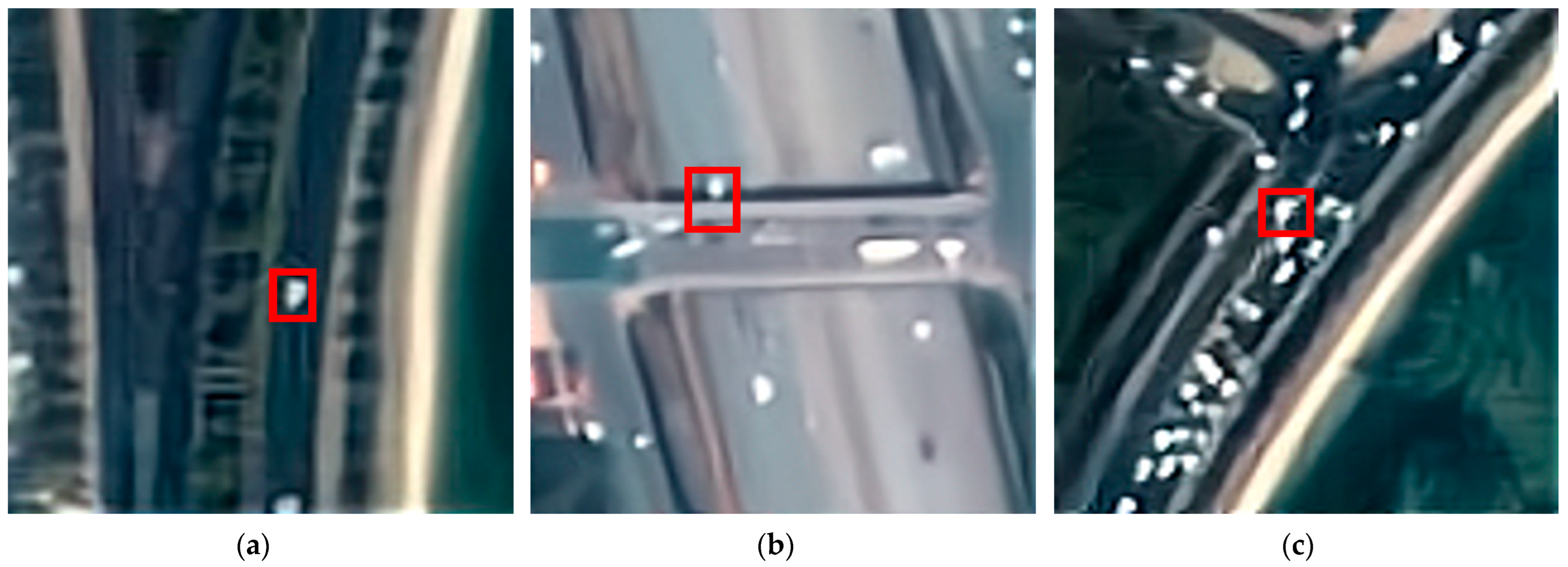
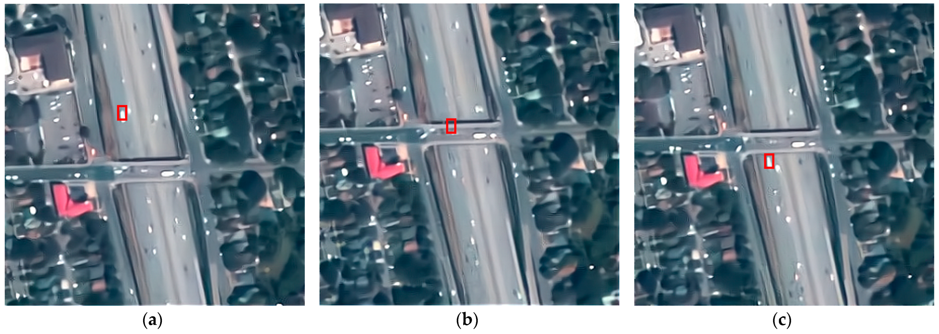
To make use of satellite videos, a variety of scholars began to pay attention to target tracking in satellite videos. As one of the most popular research directions, target tracking aims to locate the target and calculate the target trajectory [2]. However, compared with target tracking in traditional videos, target tracking in satellite videos faces more severe challenges. For example, the targets in satellite videos often have lower resolution, which accounts for only dozens of pixels. From Figure 1a, we can see that the car is just a point. In addition, occlusion is also a great challenge for satellite video tracking. The target has been occluded in Figure 1b, which is very unfavourable to the whole tracking process and may make it difficult for the algorithm to track the target again. Finally (see Figure 1c for an example), the target is much like the backdrop, which makes the target hard to distinguish. In this case, there is a great possibility that tracking drift will occur.
To date, many methods for target tracking have been presented. All are roughly classified into generative methods [3,4,5] and discriminant methods [6,7,8,9,10,11,12,13,14,15,16]. The generative methods generate a target template by extracting the representation information of the target and searching the area resembling the template. One obvious disadvantage of generative methods is that they only use the target information and ignore the role of the background. Different from generative methods, discriminant methods treat target tracking as a classification task with positive and negative samples, in which the target is a positive sample and the background is a negative sample. Because discriminant methods obtain robust tracking performance, discriminant methods have become the mainstream tracking methods.
Recently, two kinds of popular discriminant methods are deep learning (DL) based [6,7,8] and correlation filter (CF) based [9,10,11,12,13,14,15,16]. DL-based methods use the powerful representation ability of convolution features to realise target tracking. The method using hierarchical convolutional features (HCF) [6] obtains great tracking performance by using features extracted from the VGG network. Fully-convolutional Siamese networks (SiamFC) [7] use a Siamese network to train a similarity measure function offline and select the target most similar to the template. Voigtlaender et al. [8] present Siam R-CNN, a Siamese re-detection architecture, which unleashes the full power of two-stage object detection approaches for visual object tracking. In addition, a novel tracklet-based dynamic programming algorithm is combined to model the full history of both the object to be tracked and potential distractor objects. However, DL-based methods require abundant data for training. In addition, millions of parameters make it difficult for DL-based methods to achieve real-time tracking performance.
The CF-based methods transform the convolution operation into the Fourier domain through a Fourier transform, which greatly speeds up the calculation. In this case, CF-based methods are better suited for target tracking in satellite videos. The minimum output sum of squared error (MOSSE) [9] applies a correlation filter to target tracking for the first time. Due to the extremely high tracking speed of MOSSE, CF-based methods have been developed. The most famous correlation filter is the kernel correlation filter (KCF) [10], which defines the multichannel connection mode and enables the correlation filter to use various features. However, KCF is often arduous to track the target with scale change accurately. To settle the impact of scale change on the performance of the tracker, the scale adaptive kernel correlation filter (SAMF) [11] introduces scale estimation based on KCF. To make the tracker better describe the target, a convolution feature is used in correlation filtering in [12]. The background-aware correlation filter (BACF) [13] can effectively simulate the change in background with time by training real sample data. Tang et al. proposed a multikernel correlation filter (MKCF) [14] and an effective solution method. The hybrid kernel correlation filter (HKCF) [15] adaptively uses different features in the ridge regression function to improve the representation information of the target. Although the performance gradually improves, the speed advantage of the correlation filter also gradually decreases. To strike a balance between performance and speed, the efficient convolution operator (ECO) [16] introduces a factorised convolution operator to reduce the number of parameters, which can reduce computational complexity. However, the above methods cannot track the occluded target. In addition, the boundary effects caused by cyclic sampling is also a great challenge to the abovementioned methods.
Inspired by the correlation filter with motion estimation (CFME) [17], we propose a motion estimation algorithm combining the Kalman filter [18] and an inertial mechanism [19]. Because the target in the satellite videos performs uniform linear motion in most cases, the Kalman filter can accurately calculate the location of the target. However, in some cases, the trajectory of the target bends, and the position predicted by Kalman filter is no longer accurate. Therefore, we use an inertial mechanism to correct the position predicted by Kalman filter. The motion estimation algorithm not only places the target in the centre of the image patch to mitigate the boundary effects but also tracks the occluded target. Furthermore, considering the low target resolution in satellite videos, we use the HOG and OF features to improve the representation information of the target. However, background noise is inevitably introduced when fusing features. To weaken the interference of background noise on tracking performance, we introduce the disruptor-aware mechanism used in [20].
This paper makes the following contributions:
- We propose a motion estimation algorithm that combines the Kalam filter and an inertial mechanism to mitigate the boundary effects. Moreover, the motion estimation algorithm can also be used to track the occluded target;
- We fuse the HOG feature and OF feature to improve the representation information of the target;
- We introduce a disruptor-aware mechanism to attenuate the interference of backdrop noise.
2. Materials and Methods
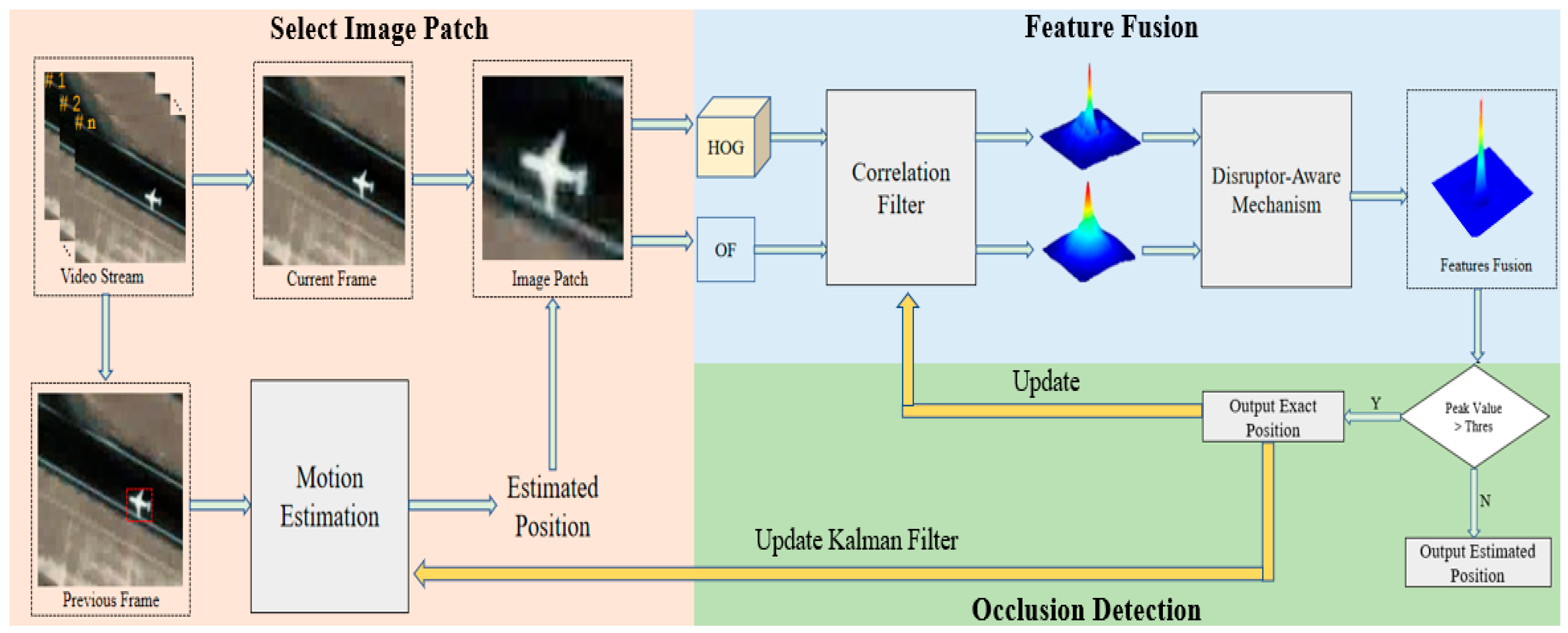
A flowchart of our algorithm is shown in Figure 2. Based on KCF [10], our algorithm includes a motion estimation algorithm, feature fusion and a disruptor-aware mechanism. It is noted that we artificially give the position of the target in the first frame, and the proposed algorithm tracks the target according to the position of the target in the first frame. First, we use a motion estimation algorithm to calculate the location of the target in the present time. Second, the image patch is cropped according to the predicted position. Third, the HOG and OF features of the image patch are extracted, and their response maps are denoised by a disruptor-aware mechanism. Fourth, feature fusion is carried out, and the maximum response value is calculated. If the peak value of the response patch is greater than the threshold, then the location predicted by the correlation filter is output; otherwise, the location calculated by the motion estimation algorithm is output.
2.1. Introduction of KCF Tracking Algorithm
KCF trains a detector to detect the target. It constructs training samples by cyclic sampling of the central target. Assume that is one-dimensional data. can be obtained by a cyclic shift of , which is expressed as . All circular shift results of are spliced into a cyclic matrix , which can be expressed by the following equation:
Cyclic matrices have the following properties:
where is the discrete Fourier transform (DFT) matrix. means conjugate transpose, and is the DFT transformation of . The diagonal matrix is shown as .
KCF uses ridge regression to train a classifier. At the same time, the label function is a Gaussian function in which the value of the centre point is 1 and the convenient value gradually decays to 0. It initialises the filter by solving , which can minimise the difference between training sample and label . The objective function is
where is a regularisation factor.
According to Equation (3), we can obtain the following equation:
where is the identity matrix. Using the properties of the Fourier transform and substituting Equation (2) into Equation (4), we can obtain Equation (5).
where , , and are the DFT of , , and respectively. is the complex conjugation of . The operator is the Hadamard product of matrix.
The performance of the tracker can be improved by using the kernel trick. Suppose the kernel is . can be written as
For most of the kernel function, the properties of Equation (2) still hold. Then, can be solved by
where is the DFT of , and is the trained filter. Because we make use of a Gaussian function as the label, can be shown as
where is the complex conjugation of , and is the Hadamard product of the matrix. The number of characteristic channels is represented by . is the inverse transform of the Fourier transform.
When tracking the target, the algorithm cuts out the candidate region centred on the target. Then, the response patch is calculated by
where is the representation information of the candidate region, and is the target template.
When the target is moving, the apparent characteristics of the target often vary. Therefore, to better describe the target, the correlation filter also needs to be updated dynamically. The KCF is updated by using
where is the learning rate. and are the new filter and samples, respectively.
2.2. Motion Estimation Algorithm
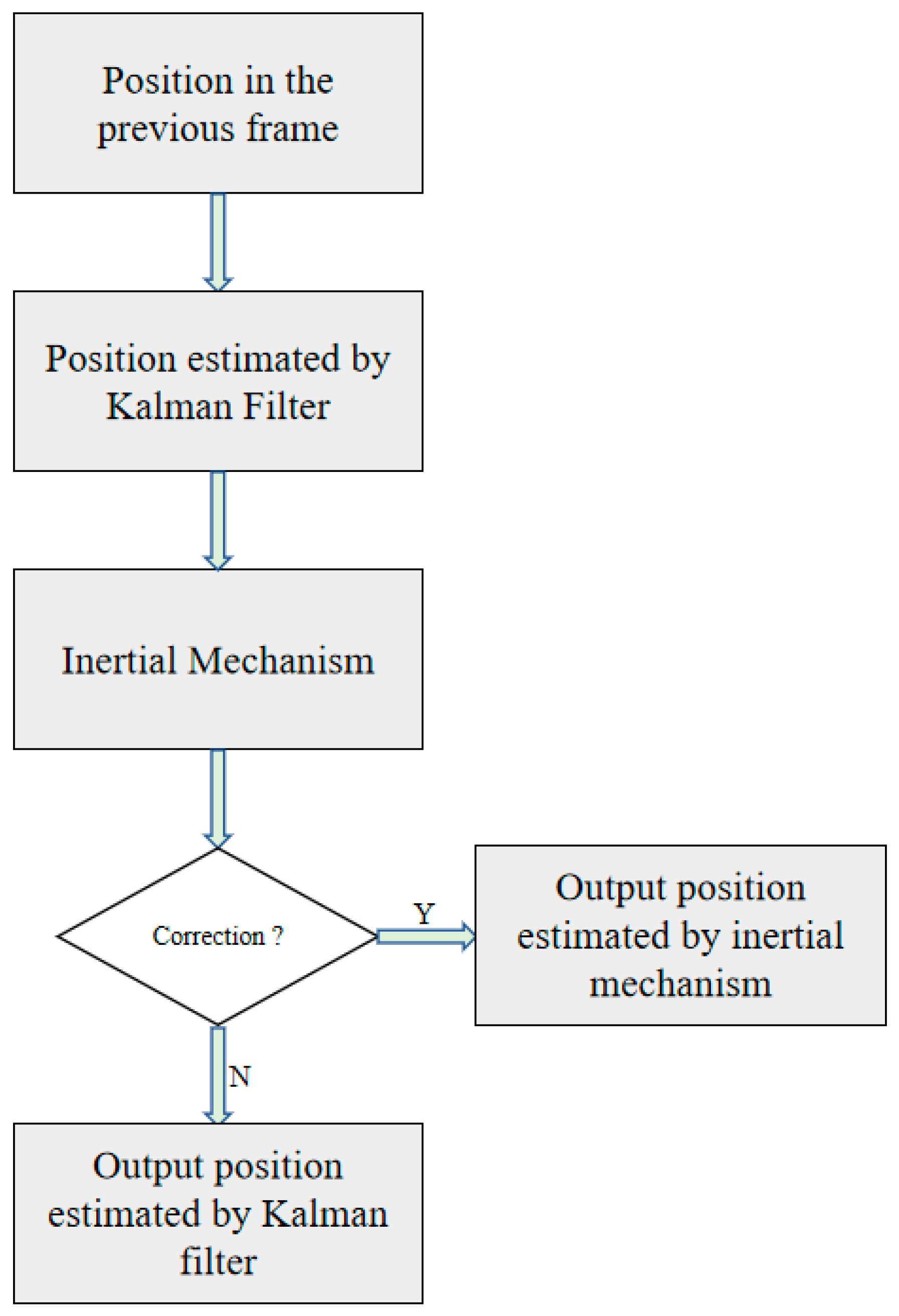
We introduce motion estimation to make our tracker work more accurately. This includes the Kalman filter [18] and an inertial mechanism [19]. Kalman filter calculates the location of the target in the current time through the location of the target in the previous frame. However, sometimes the position predicted by Kalman filter is not credible. Therefore, an inertial mechanism is used to correct the position predicted by Kalman filter. A flowchart of the motion estimation algorithm is shown in Figure 3.
2.2.1. Kalman Filter
The state and observation equations are
where is the state transition matrix in the frame, and is the observation transition matrix in the frame. and are the state vector and the observation vector, respectively. . and are the white Gaussian noise with covariance matrices and .
In our algorithm, the location of the target can be written as
where and are the abscissa and ordinate of the target, respectively. and are the horizontal velocity and vertical velocity of the target, respectively.
Because the moving distance of the target between adjacent frames is very short, we think that the target moves at a uniform speed. In this situation, the state transition matrix and the observation matrix can be expressed as
The update process of Kalman filter is as follows:
where is the state vector in frame and is the observation vector in frame . is the prediction error covariance matrix, and is the identity matrix.
2.2.2. Inertial Mechanism
A video satellite can observe the long-term motion state of the target. Different from traditional videos, the target moves linearly most of the time, and the Kalman filter can calculate the location of the target well. However, the trajectory sometimes bends. In this case, the Kalman filter cannot accurately calculate the location of the target, so an inertial mechanism is introduced to correct the location estimated by the Kalman filter. From [19], we can see that the performance of the inertial mechanism is obviously better than the Kalman filter when the target trajectory is curved.
When tracking the target in frame , position predicted by the Kalman filter is sent into the inertial mechanism. If the difference between and position predicted by the inertial mechanism is beyond the threshold, then is used to replace . can be calculated by using
where is the inertia distance. can be updated by linear interpolation:
where is the inertia factor. The threshold of the triggering inertia mechanism is related to the residual distance . can also be updated by linear interpolation:
2.3. Feature Fusion
OF can well describe the moving state of the target. Therefore, OF is well suited for satellite video tracking. OF assumes that pixels within a fixed range have identical speeds. The pixels centred on satisfy the following equation:
where are pixels centred on . , and are the partial derivatives of with respect to , , and . Equation (22) can be shown by using the matrix
where
We multiply Equation (23) left by , which can be written as
The following equation can be obtained by solving Equation (25):
The HOG feature is widely used in correlation filtering. It divides the input image into several cells according to a certain proportion and calculates the gradient in the discrete direction to form a histogram. HOG can well represent the contour features of the target. Therefore, HOG and OF can describe the target from different angles to enhance the representation information.
The peak-to-side Lobe ratio (PSR) [9] is utilised to describe the tracking performance of the tracker. The higher the PSR value, the better the tracking performance. If the value of PSR is lower than a certain value, then it can be considered that the tracking quality is poor. The calculation formula of PSR is as follows:
where , and is the maximum response value. and are the mean and variance of the sidelobe, respectively. In this paper, we use PSR to fuse the HOG feature and OF feature, which can be expressed as
where is the final response patch. and are the response patches of HOG and OF, respectively. can be shown as
where and are the PSR of the HOG response patch and OF response patch, respectively.
2.4. Disruptor-Aware Mechanism
As we all know, a smooth response patch will make the tracker achieve excellent tracking performance. However, when tracking the target, the target is easily disturbed by a similar background, which makes the response value of noise too large. This may affect the follow-up tracking performance and even lead to tracking failure. Therefore, we must remove points with abnormal response values.
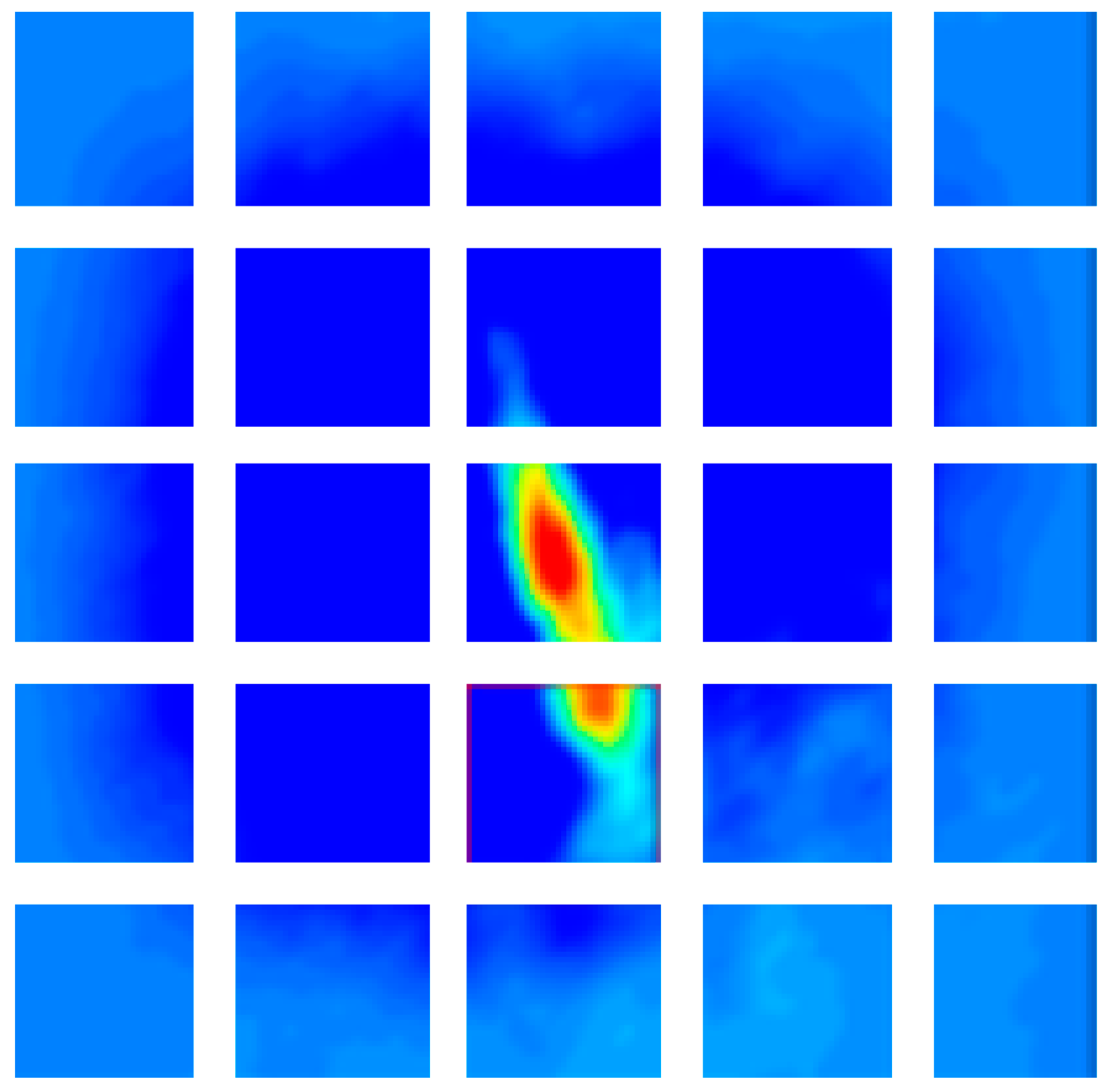
In this paper, we introduce a disruptor-aware mechanism [20] to suppress background noise. We first divide the response patch into blocks and find the local maximum of the block in the th row and th column, where . When is 5, the divided response patch is shown in Figure 4. Then, we find the global maximum and set the penalty mask of its location to 1. Finally, we set the penalty mask for other blocks through Equation (28).
where is a penalty coefficient, and is a threshold to trigger the disruptor-aware mechanism. is calculated as
By using Equations (30) and (31), we can obtain the matrix composed of penalty masks. The matrix is shown as
Finally, we can obtain the denoised response patch by dot multiplying the response patch with Equation (30).
2.5. Occlusion Detection
Because the targets in satellite videos have very low resolution, there is a great possibility that occlusion will occur, as shown in Figure 5. We can see that the movement of the car is divided into three stages.
- Before occlusion occurs, the car runs normally.
- When occlusion occurs, the car is occluded by the overpass, and the whole car disappears from view. In this case, the correlation filter often fails to track the target.
- When the occlusion ends, the car returns to our view.
To make our algorithm able to track the occluded target, we introduce an occlusion detection mechanism. The occlusion detection mechanism should be able to judge when occlusion occurs and when occlusion ends. When the target is occluded, the position predicted by the correlation filter will no longer be credible. In view of the particularity of target motion in satellite videos, we regard the position predicted by the motion estimation algorithm as the position of the target in the current frame. In addition, if we continue to update the template when the target is occluded, it is easy to cause template degradation. To prevent template degradation, the correlation filter will not be updated at this time. When the occlusion is over, we continue to output the position predicted by the correlation filter.
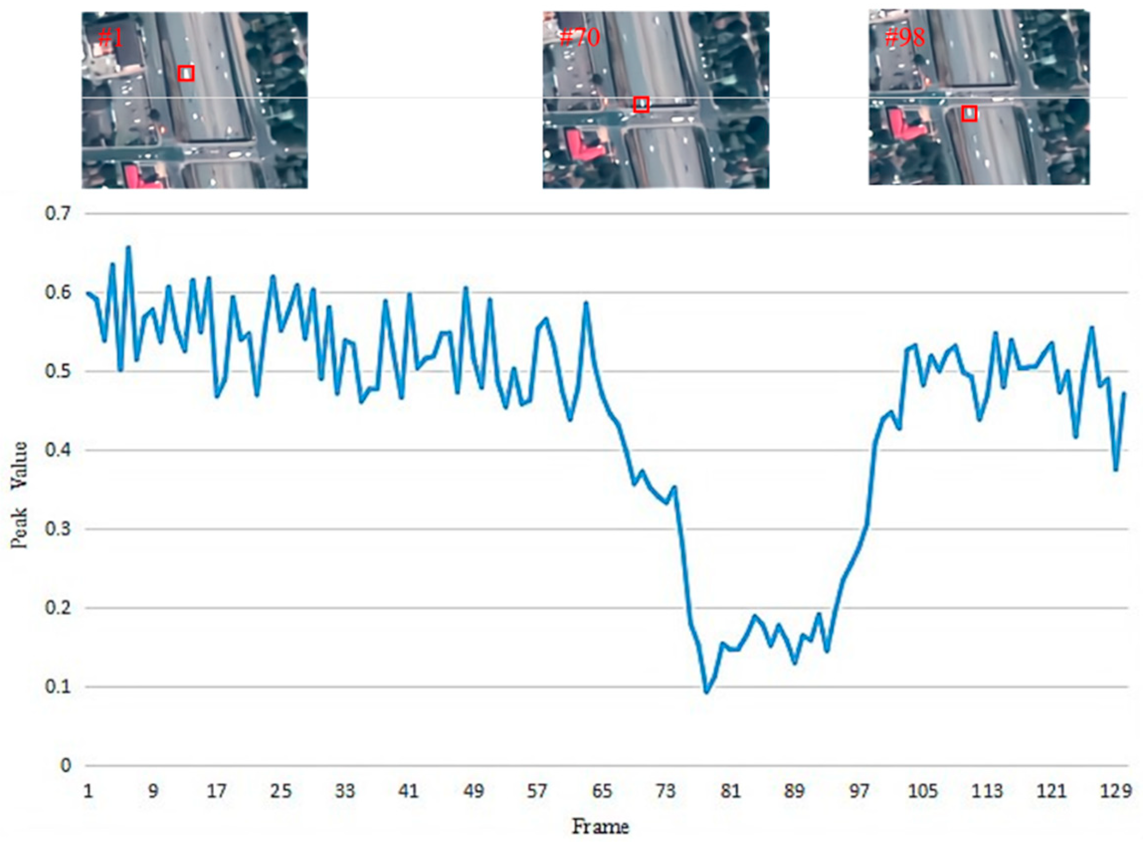
When the target is accurately tracked, it often has a large response value. In contrast, if the tracking quality is poor, then the response value of the response patch will decrease rapidly. Therefore, we use the maximum response value of the response patch to judge whether occlusion occurs. Through experiments, the threshold is set to 0.3. When the maximum response value is less than 0.3, we think that the target is occluded at this time and take the position predicted by the motion estimation algorithm as the position of the target and stop updating the template. The update process is expressed as Equation (33). Otherwise, the location predicted by the correlation filter is output.
where is the learning rate, is the trained filter and is the new filter.
3. Results
3.1. Setting of Parameters
Our algorithm involves many parameters. To facilitate viewing the parameters in this paper, this part introduces the details on the setting of parameters. The specific settings of the parameters involved in this paper are listed in Table 1.
3.2. Setting of Threshold to Detect Occlusion
We use the peak value to judge whether the target is occluded. From Figure 6, we can see that the peak value decreases rapidly when occlusion occurs. What is more, when the peak value is lower than 0.3, the whole car disappears from view.
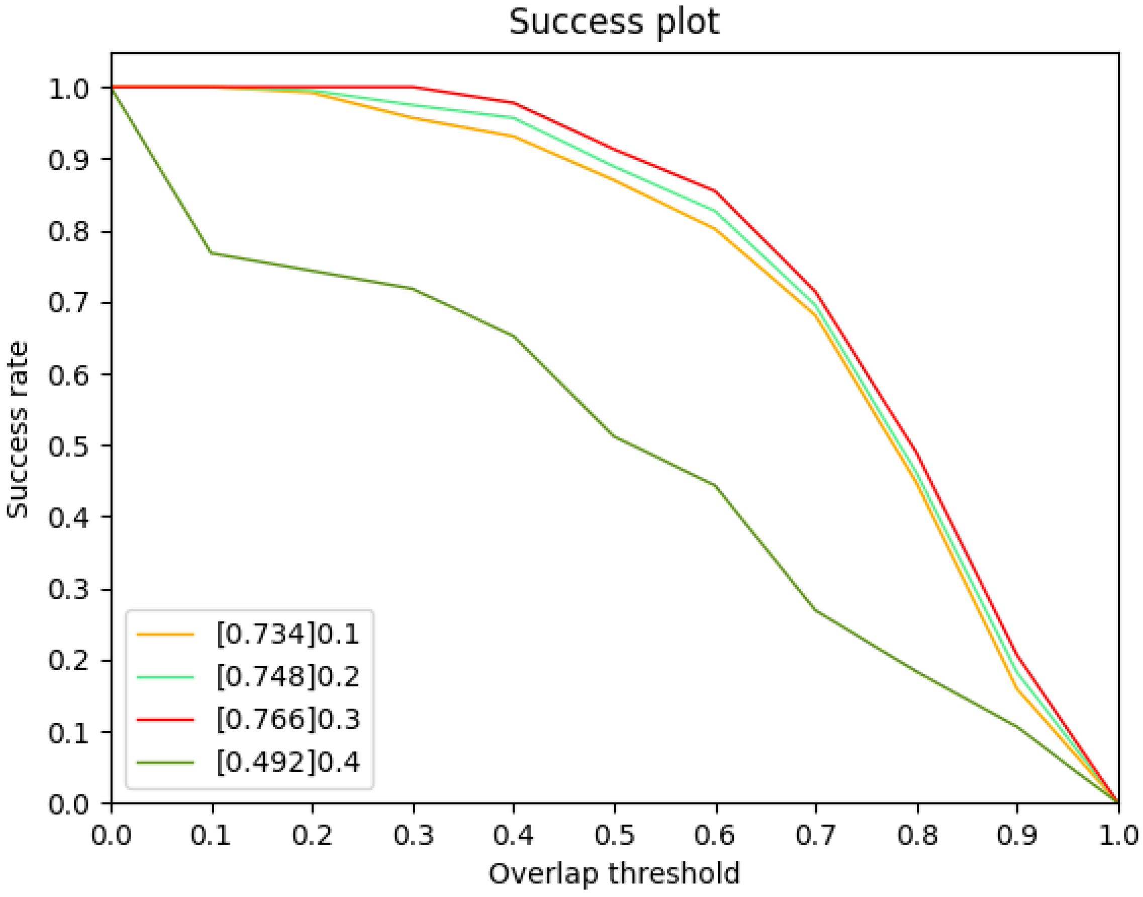
We use a grid search to select the best performing threshold from [0.1, 0.2, 0.3, 0.4]. The success plot on every threshold is shown in Figure 7. The AUC is highest when the threshold is 0.3, therefore we choose 0.3 as the threshold.
3.3. Datasets and Compared Algorithms
Some datasets are provided by the Jilin-1 satellite, and the other part is public data [21]. We select nine videos to test our tracker. In this paper, the results of five representative videos are shown. Video 1–4 are provided by Jilin-1 satellite and video5 is public data. The targets tracked in the videos include planes, cars and ships. In addition, the tracked target has the following challenges: low resolution, global occlusion and fast rotation. The detail information about the dataset is listed in Table 2. To measure the performance of our algorithm, we select the following popular algorithms for comparison: CFME, MOSSE, KCF, multiple instance learning (MIL) [22], BOOSTING [23] and median flow (MEDIANFLOW) [24]. The motion estimation algorithm of our tracker is inspired by CFME. KCF is the baseline of our tracker. MOSSE is the first algorithm to use correlation filtering for tracking. Other algorithms are classical tracking algorithms.
3.4. Evaluation Metrics
The centre location error (CLE) and Tanimoto Index [25] are the two most commonly used evaluation metrics in target tracking. CLE means the Euclidean distance between the real position and the predicted position. The Tanimoto Index is used to describe the proportion of overlapping area between the predicted area and real area in the total area, which can be shown as
where and are the ground truth position and the position predicted by the algorithm, respectively. and denote the union and intersection of two positions.
To better compare the performance of different algorithms, we use additional metrics, such as FPS, precision score, precision plot, success score, success plot and area under the curve (AUC). FPS is the number of frames that the tracker can process per second. The precision score is used to describe the proportion of frames whose CLE is less than the threshold (5 pixels) in the total number of frames. The precision plot is a curve according to the precision score. The success score denotes the proportion of frames whose overlap ratio is larger than the threshold (0.5) in the total number of frames. The success plot is drawn by success score. AUC describes the offline area of the success plot. The larger the AUC is, the better the tracking effect. We rank each tracker through the AUC.
3.5. Comparative Experiments
3.5.1. Quantitative Analysis
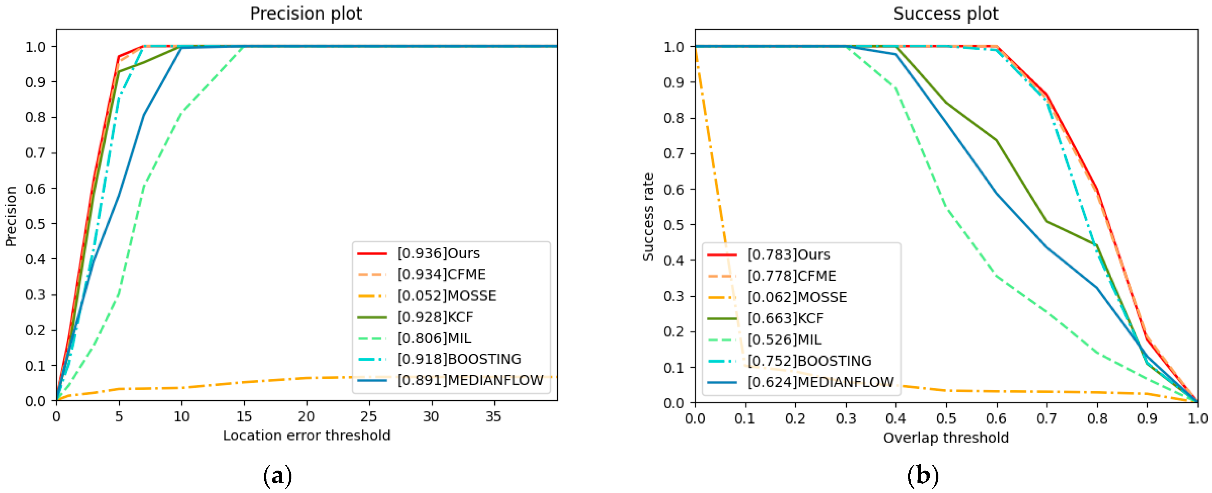
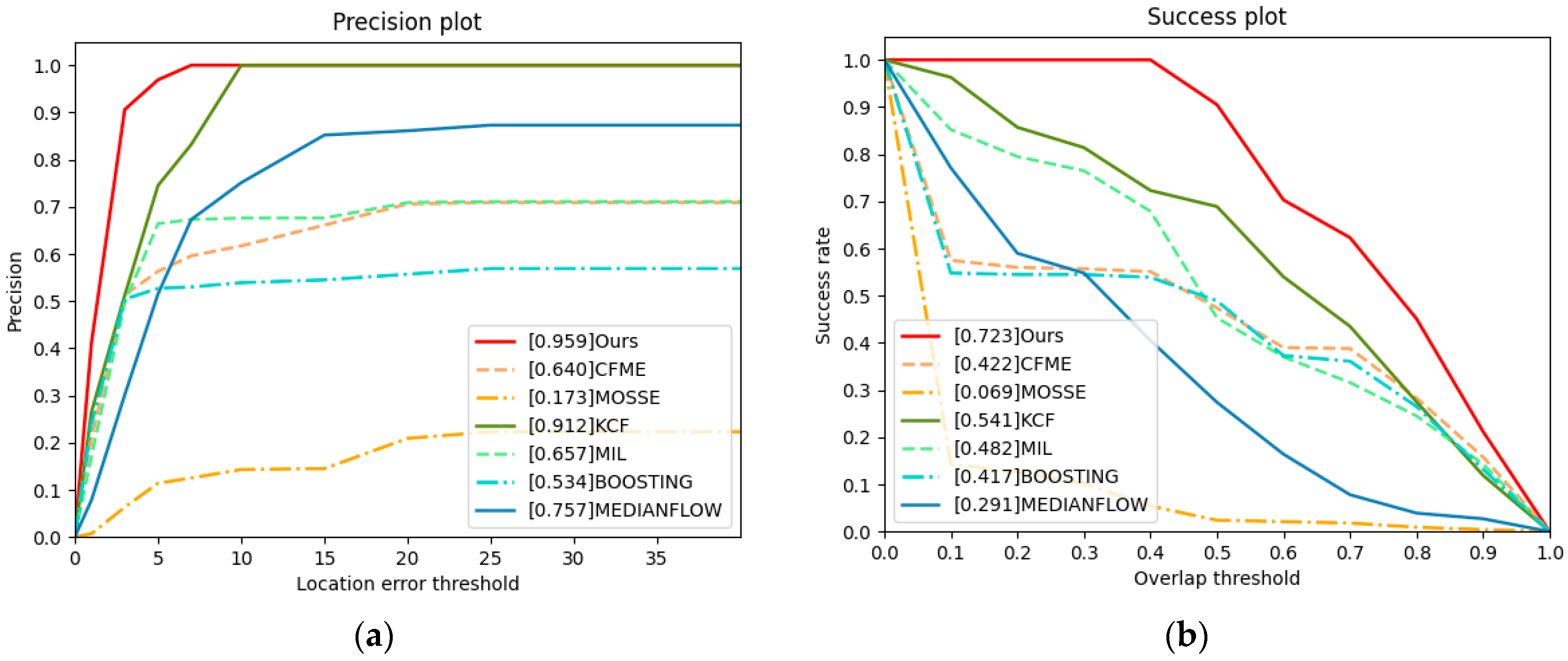
We first choose the plane and ship of satellite videos as the tracked targets. The results are shown in Figure 8. Because our algorithm and CFME alleviate the boundary effects, the tracking performance is obviously better than that of other algorithms. However, according to Table 3 and Table 4, our algorithm achieves higher tracking accuracy than CFME. The reason is that our algorithm uses the HOG and OF features, while CFME only uses the HOG feature. Therefore, our algorithm can extract more information about the target.
For the KCF, which also uses the HOG feature, good performance is also obtained, and KCF ranks third, while MOSSE uses the grey feature of the target. Due to the low resolution of the target in satellite videos, the grey feature cannot accurately describe the target, so the performance of MOSSE is not ideal. Therefore, in satellite video tracking, the features have a wonderful impact on tracking performance. Our algorithm utilises two complementary features and obtains great performance.
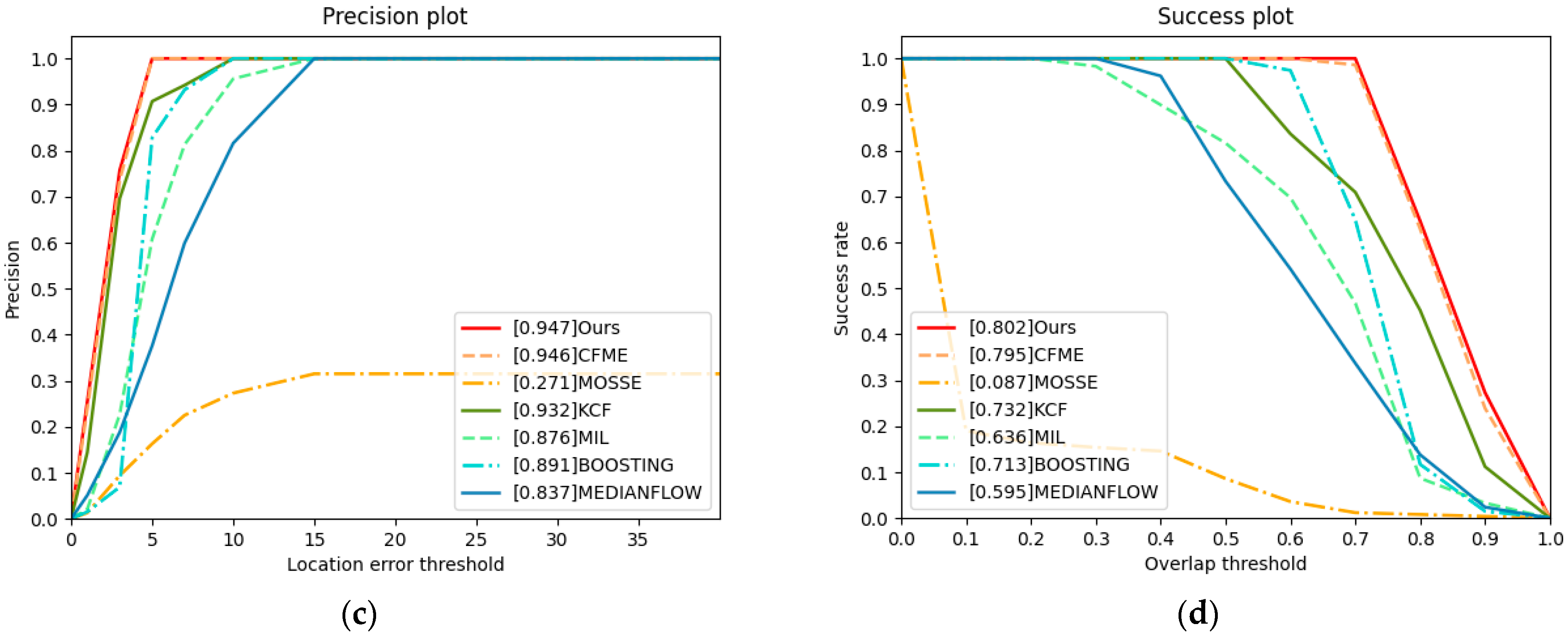
Occlusion is the most common challenge in target tracking. Especially in satellite video tracking, the tracked target is often completely occluded. Therefore, to validate the tracking performance of our algorithm for occluded targets, we specifically select a video with global occlusion. Table 5 and Figure 9 show that both our algorithm and CFME have achieved great performance. Our algorithm and CFME can track the occluded target through the occlusion detection mechanism. The other algorithms fail to track. The AUC of our algorithm is 0.704, and the AUC of CFME is 0.698. KCF ranks third, but its AUC is only 0.426. Before the target is occluded, the KCF can accurately track the target. However, the KCF gradually loses the target after the target is occluded. In this case, our algorithm and CFME are obviously superior to other algorithms.
From Table 6 and Figure 10, we can see that the performance of our algorithm is the best of all algorithms. The tracked target in this video has low resolution and rotates fast at the same time. The performance of CFME has decreased considerably and finally fails to track. Because the target rotates fast, the response value at a certain time is lower than the occlusion threshold of CFME. Under these circumstances, the occlusion detection mechanism of CFME is activated. CFME considers the location predicted by the motion estimation mechanism as the real location, which may lead to tracking failure. In addition, the performance of KCF is better than that of CFME. When the target rotates fast, the motion estimation algorithm of CFME has a negative impact and leads CFME to fail to track. Making a comparison with CFME, the precision score of our algorithm is increased by approximately 0.406, the success score of our algorithm increases by approximately 0.431 and the AUC of our algorithm increases by approximately 0.301. In summary, when the tracked target rotates fast, our algorithm can still track the target accurately.
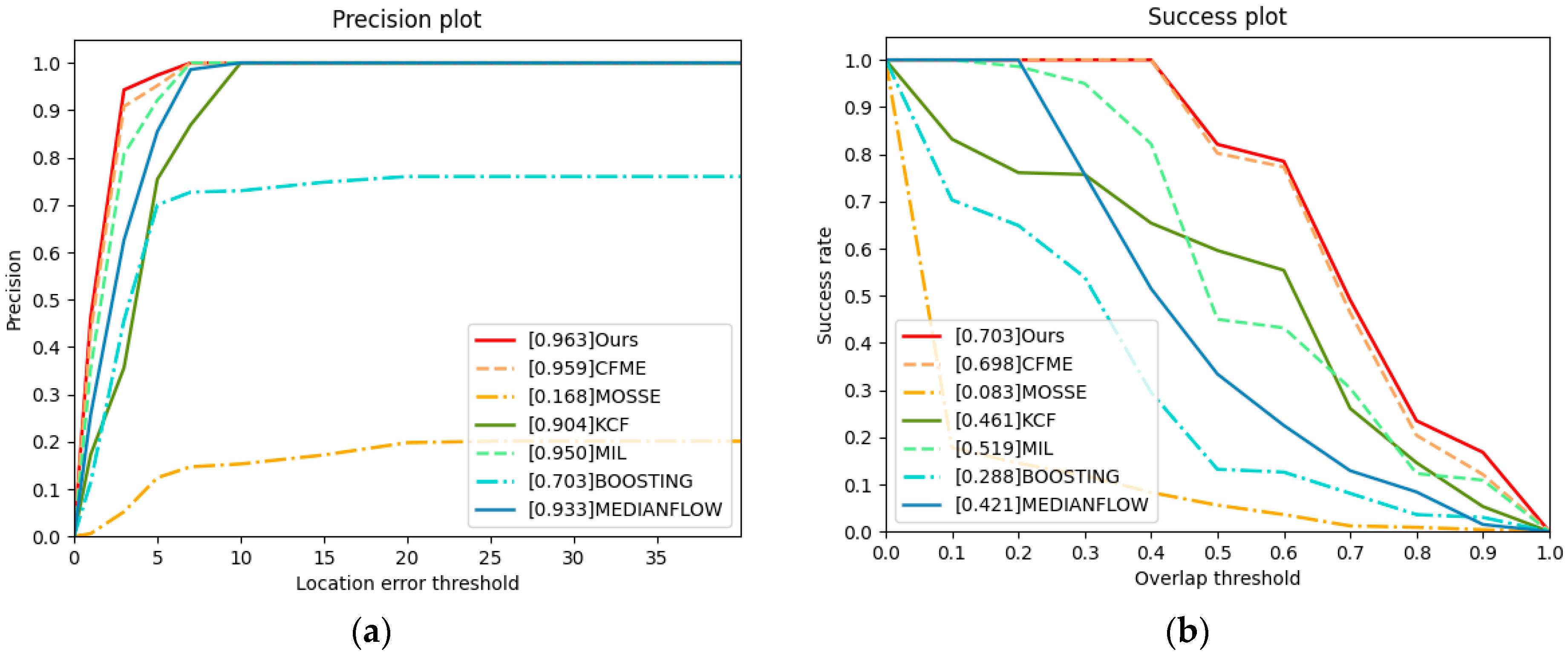
To test the proposed method, we use a video from other sensors. From Table 7 and Figure 11, we can see that our algorithm achieves the best performance. Because the target in video5 is moving in a uniform liner motion, CFME effectively alleviates the boundary effect through motion estimation algorithm and performs well. Due to the use of HOG feature and OF feature, the performance of our algorithm is better than CFME.
3.5.2. Qualitative Analysis
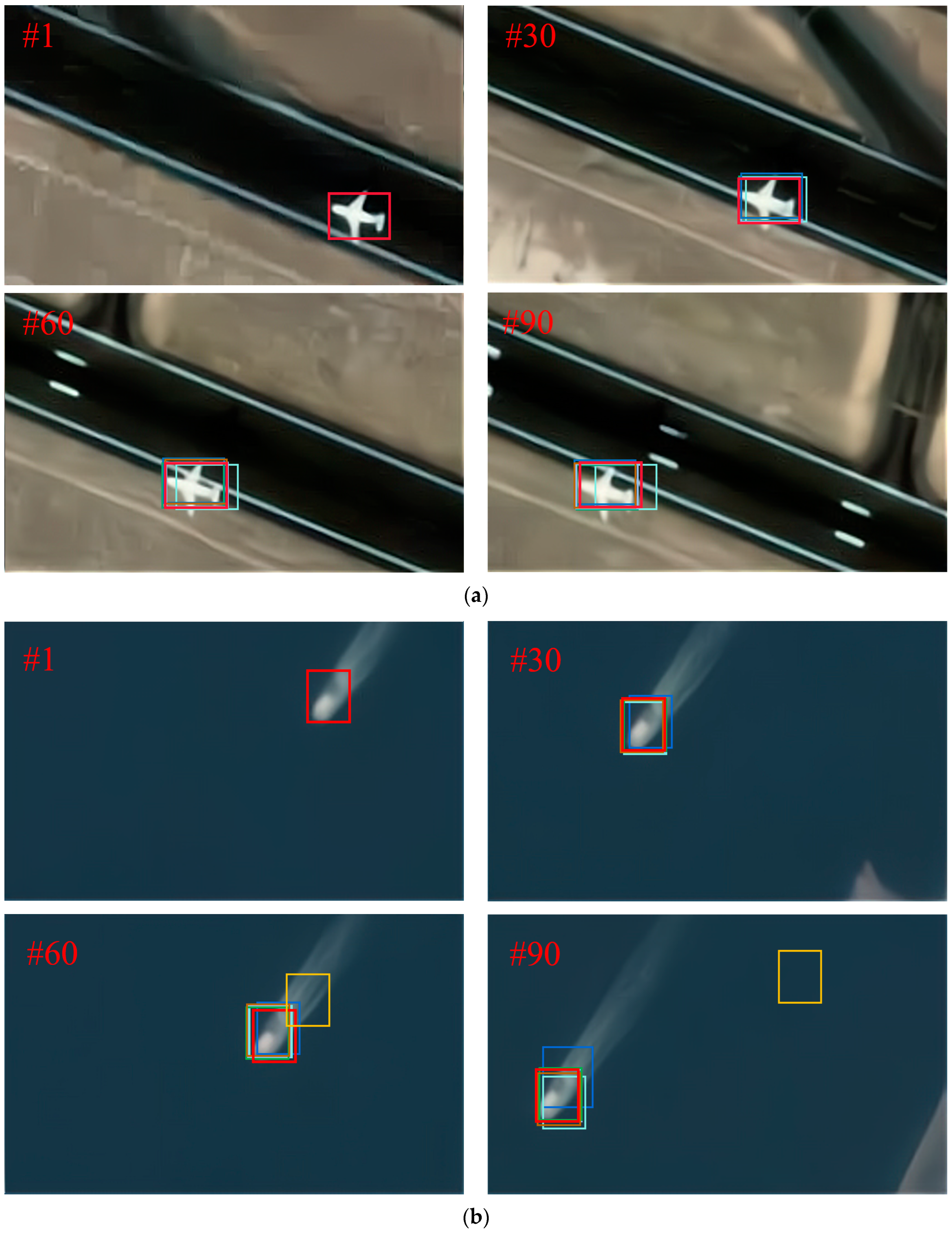
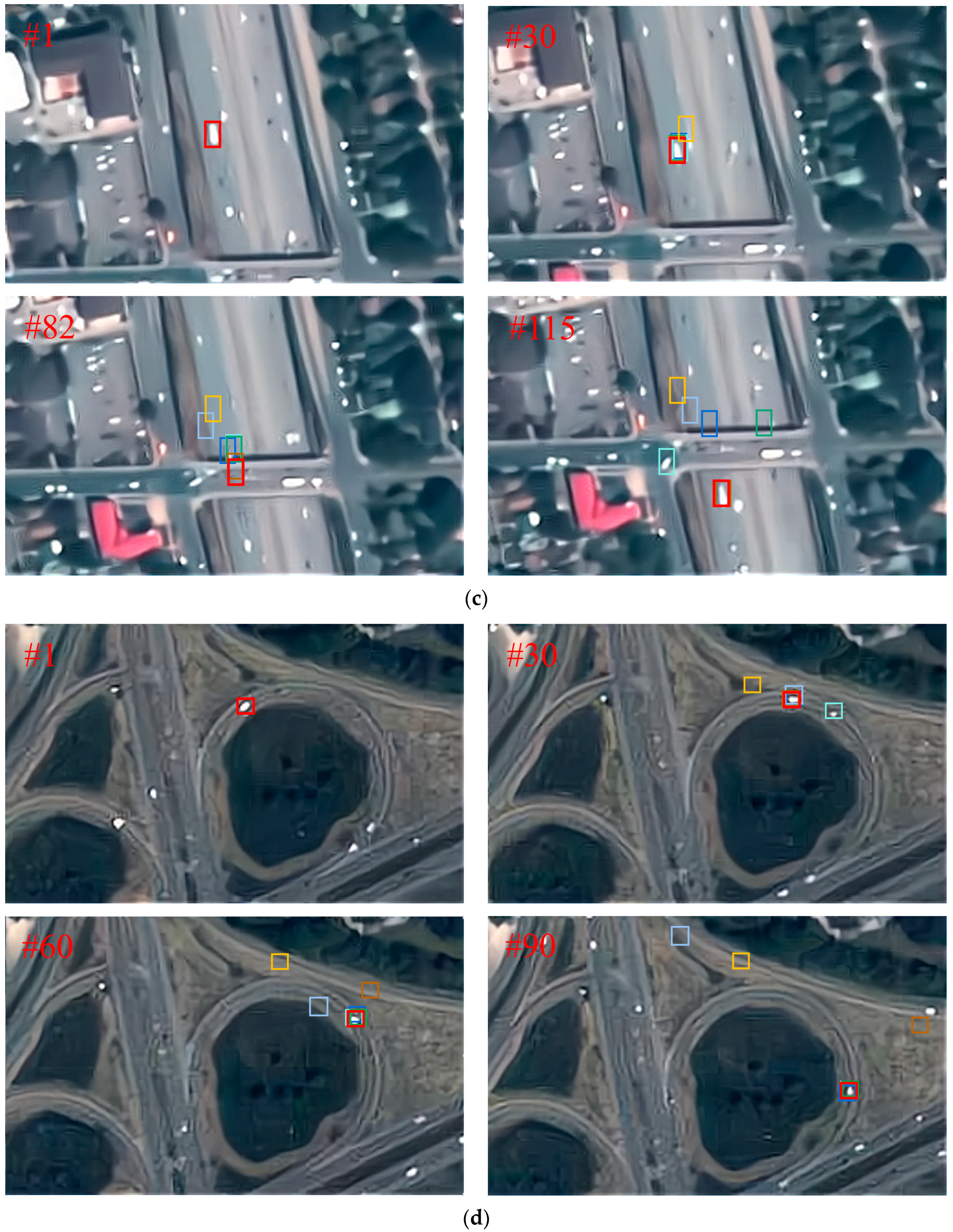
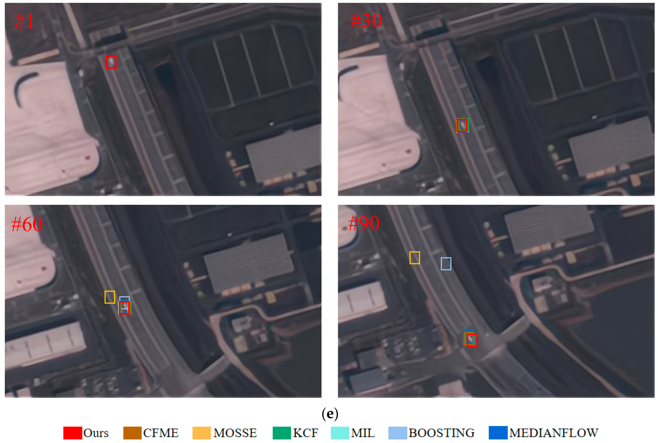
Figure 12 represents the visualised results. In Figure 12a,b, there is no severe challenge to the tracked target, and the size of the target is large. Therefore, our algorithm and CFME perform well. In addition, due to the use of HOG features, KCF also achieved good performance and ranks third. However, KCF is unable to track the occluded target. From Figure 12c, we can see that when the target crosses the overpass, it is completely occluded and disappears in the field of vision. At this time, KCF cannot find the location of the target and fails to track the target. However, our algorithm and CFME can predict the position of the target through motion estimation. Thus, even if the target is completely occluded, our algorithm and CFME can still track the target. When the target appears again, our algorithm and CFME can track the target. However, KCF has been hovering beside the overpass. Owing to motion estimation, our algorithm and CFME can solve the occlusion problem well. However, CFME only uses Kalman filter to calculate the location of the next frame. If fast rotation occurs, then the position predicted by CFME will often deviate from the real position of the target and eventually lead to tracking failure. According to Figure 12d, our algorithm can accurately track rotating targets. Although MIL achieved good tracking accuracy for rotating targets, when similar targets appear around them, MIL has a high probability of tracking the wrong target. From Figure 12e, we can see that our algorithm still achieves the best performance when we use a video from other sensors.
3.6. Ablation Experiment
To verify the significance of the motion estimation algorithm M1, feature fusion M2 and the disruptor-aware mechanism M3, we perform the following experiments: “Baseline,” “Baseline + M1,” “Baseline + M1 + M2” and “Baseline + M1 + M2 + M3.” Among them, “Baseline” denotes the KCF tracker. The results are shown in Table 8. We can see that M1, M2 and M3 improve the performance of the KCF in precision score, success score and AUC. Moreover, compared with KCF, our algorithm improves the performance by 0.198, 0.170 and 0.178 in precision score, success score and AUC, respectively.
4. Discussion
4.1. Analysis of Proposed Algorithm
4.1.1. Boundary Effects
CF-based method utilises a periodic assumption of the training samples to efficiently learn a classifier on all patches in the target neighbourhood. However, the periodic assumption also introduces unwanted boundary effects, which severely degrade the quality of the tracking model. In the training stage, because the training samples are obtained by cyclic shifts of the central image, they all have boundary effects except for the central image. When tracking the target, if the moving speed of the target is too fast, then tracking drift easily occurs. Most algorithms add a cosine window to the image to weaken the influence of the boundary effects on the tracking performance. However, this also shields the background information and reduces the discrimination ability of the classifier. To alleviate the boundary effects, a spatially regularised correlation filter (SRDCF) [26] introduces a spatial regularisation component. In addition, Galoogahi et al. [27] used larger image blocks and smaller filters to increase the proportion of real samples. However, its computational complexity is unaffordable.
Considering that the moving objects in the satellite videos are vehicles, planes or ships, the acceleration of these objects is not particularly large, which means that the motion state of these objects does not change in a short period of time. Therefore, the movement of objects in satellite videos is usually regular. Inspired by the observation, we propose a motion estimation algorithm that combines Kalman filter and inertial mechanism to alleviate the boundary effects.
From Table 8, it is obvious that compared with the baseline, i.e., KCF, the precision score of “baseline+M1” is increased by approximately 0.162, the success score of “baseline+M1” is increased by approximately 0.147 and the AUC of “baseline+M1” is increased by approximately 0.157. By alleviating the boundary effects, the performance of our algorithm is obviously better than that of KCF.
4.1.2. Target Occlusion
With the development of the commercial satellite industry, satellite video tracking has attracted extensive attention. To track the target in satellite videos, many methods have been developed. HKCF [15] uses an adaptive feature fusion method to enhance the representation information of the target. Du et al. proposed a multiframe optical flow tracker (MOFT) [28] that fuses the Lucas–Kanade optical flow method with the HSV colour system. A Gabor filter is utilised to strengthen the contrast between the target and background in [29]. A detection algorithm based on a local noise model [30] is proposed to track city-scale moving vehicles. Although the above algorithms can track the target well, these algorithms often fail if occlusion occurs. Through the use of motion estimation, our algorithm can not only track the target robustly but also track the target that reappears after being occluded.
From Figure 12c, we can see that when the target is occluded, the occlusion detection mechanism of our algorithm is activated and our algorithm can go on tracking the target. In this case, our algorithm tracks the target through the motion estimation algorithm, and the model will not be updated at this time, which can avoid model degradation. When the target reappears, our algorithm tracks the target through the correlation filter.
4.2. Future Work
4.2.1. Satellite Video Tracking by Deep Learning
Deep learning has made rapid development in recent years, and is widely used in various fields, such as computer vision, natural language processing and so on. As one of the most popular research directions, object tracking aims to locate the target and calculate the trajectory. Presently, many DL-based methods are used in object tracking, and have achieved excellent performance. But compared with object tracking in traditional videos, object tracking in satellite videos faces more severe challenges.
Some methods have been proposed for satellite video tracking. A regression network is used to combine a regression model with convolutional layers and a gradient descent algorithm in [31]. The regression network fully exploits the abundant background context to learn a robust tracker. In [32], an action decision-occlusion handling network based on deep reinforcement learning is built to achieve low computational complexity for object tracking under occlusion. Besides, the temporal and spatial context, the object appearance model, and the motion vector are adopted to provide the occlusion information. The above methods have achieved great performance. However, the timing performance is not ideal.
Because of the low resolution, the manual features cannot accurately describe the target in satellite videos. It can be observed that compared with manual features, convolution features have better representation ability. In future work, deep learning will be used for object tracking in satellite videos. Meanwhile, the timing performance also has to be considered.
4.2.2. Multi-Object Tracking in Satellite Videos
Multi-object tracking (MOT) aims to assign an ID to each target in the video and calculate the trajectory of each target. According to whether there is a model, MOT is classified into a model-free method and tracking by detection method. Considering the great performance, the tracking by detection method [33,34,35,36] has been rapidly developing.
Presently, deep learning is widely used in MOT and performs well. However, MOT in satellite videos still faces great challenges. On the one hand, due to the lack of satellite datasets and strong confidentiality, it is difficult to have enough data to train the model. On the other hand, the targets in satellite videos are very similar, which may lead to frequent ID switch. He et al. [21] propose an end-to-end online framework that models MOT as a graph information reasoning procedure from the multitask learning perspective. However, most point-like objects are very similar to the background in space, easily leading to omissions in detection. Aguilar et al. [37] propose a patch-based convolutional neural network (CNN) that focuses on specific regions to detect and discriminate nearby small objects. Besides, an improved Gaussian mixture-probability hypothesis density filter is used for data-association. Due to the patch selection and CNN inference, the computational burden is increased.
With the development of commercial satellite industry and deep learning, more open satellite data are available and more efficient algorithms are proposed, which will advance the development of relevant research work. Therefore, MOT in satellite videos will play an important role in the future.
5. Conclusions
In this paper, we proposed a multi-feature correlation filter with motion estimation to track the target in satellite videos. This has obvious superiority over representative methods. First, a motion estimation algorithm that combines the Kalman filter and inertial mechanism was employed to alleviate the boundary effects and track occluded targets. In addition, considering the low resolution of targets in satellite videos, HOG features and OF features were integrated to improve the presentation information of the target. Finally, a disruptor-aware mechanism was introduced to suppress the interference of background noise. Several experiments were carried out to prove the effectiveness of our algorithm. Future work will focus on applying deep learning to satellite video tracking and studying MOT in satellite videos.
Author Contributions
Conceptualisation, Y.Z. (Yan Zhang), D.C. and Y.Z. (Yuhui Zheng); methodology, Y.Z. (Yan Zhang); software, Y.Z. (Yan Zhang); validation, Y.Z. (Yan Zhang); formal analysis, Y.Z. (Yan Zhang); investigation, Y.Z. (Yan Zhang); resources, Y.Z. (Yan Zhang), D.C. and Y.Z. (Yuhui Zheng); data curation, Y.Z. (Yan Zhang); writing—original draft, Y.Z. (Yan Zhang); writing—review and editing, Y.Z. (Yan Zhang), D.C. and Y.Z. (Yuhui Zheng); visualisation, Y.Z. (Yan Zhang); supervision, Y.Z. (Yan Zhang), D.C. and Y.Z. (Yuhui Zheng); project administration, Y.Z. (Yan Zhang); funding acquisition, Y.Z. (Yuhui Zheng). All authors have read and agreed to the published version of the manuscript.
Funding
This research was supported in part by the Natural Science Foundation of Jiangsu Province under Grant BK20211539; in part by the National Natural Science Foundation of China under Grants 61972206, 62011540407 and J2124006; in part by the 15th Six Talent Peaks Project in Jiangsu Province under Grant RJFW-015; in part by the Qing Lan Project; and in part by the PAPD fund.
Data Availability Statement
All data included in this study are available upon request by contact with the corresponding author.
Conflicts of Interest
The authors declare no conflict of interest.
References
- Li, X.; Guo, Q.; Lu, X. Spatiotemporal statistics for video quality assessment. IEEE Trans. Image Process. 2016, 25, 3329–3342. [Google Scholar] [CrossRef] [PubMed]
- Luo, Y.; Liang, Y.; Wang, Y. Traffic flow parameter estimation from satellite video data based on optical flow. Comput. Eng. Appl. 2018, 54, 204–207. [Google Scholar]
- Birchfield, S.T.; Rangarajan, S. Spatiograms versus histograms for regio-based tracking. In Proceedings of the 2005 IEEE Conference on Computer Vision and Pattern Recognition (CVPR), San Diego, CA, USA, 20–25 June 2005; pp. 1158–1163. [Google Scholar]
- Nummiaro, K.; Koller-Meier, E. Object tracking with an adaptive color-based particle filter. In Proceedings of the Joint Pattern Recognition Symposium, Berlin, Germany, 16–19 September 2002; pp. 353–360. [Google Scholar]
- Possegger, H.; Mauthner, T.; Bischof, H. In defense of color-based model-free tracking. In Proceedings of the 2015 IEEE Conference on Computer Vision and Pattern Recognition (CVPR), Boston, MA, USA, 7–12 June 2015; pp. 2113–2120. [Google Scholar]
- Ma, C.; Huang, J.; Yang, X.; Yang, M. Hierarchical convolutional features for visual tracking. In Proceedings of the 2015 IEEE International Conference on Computer Vision (ICCV), Santiago, Chile, 13–16 December 2015; pp. 3074–3082. [Google Scholar]
- Bertinetto, L.; Valmadre, J.; Henriques, J.F.; Vedaldi, A.; Torr, P.H.S. Fully-convolutional siamese networks for object tracking. In Proceedings of the European Conference on Computer Vision Workshop (ECCVW), Amsterdam, The Netherlands, 8–16 October 2016; pp. 850–865. [Google Scholar]
- Voigtlaender, P.; Luiten, J.; Torr, P.H.S. Siam R-CNN: Visual tracking by re-detection. In Proceedings of the 2020 IEEE Conference on Computer Vision and Pattern Recognition (CVPR), Seattle, WA, USA, 13–19 June 2020. [Google Scholar]
- Bolme, D.S.; Beveridge, J.R.; Draper, B.A. Visual object tracking using adaptive correlation filters. In Proceedings of the 2010 IEEE Conference on Computer Vision and Pattern Recognition (CVPR), San Francisco, CA, USA, 13–18 June 2010; pp. 2544–2550. [Google Scholar]
- Henriques, J.F.; Caseiro, R.; Martins, P.; Batista, J. High-speed tracking with kernelized correlation filters. IEEE Trans. Pattern Anal. Mach. Intell. 2015, 37, 583–596. [Google Scholar] [CrossRef] [PubMed] [Green Version]
- Li, Y.; Zhu, J. A scale adaptive kernel correlation filter tracker with feature integration. In Proceedings of the European Conference on Computer Vision Workshop (ECCVW), Zurich, Switzerlan, 6–12 September 2014; pp. 254–265. [Google Scholar]
- Danelljan, M.; Hager, G.; Khan, F.S.; Felsberg, M. Convolutional features for correlation filter based visual tracking. In Proceedings of the 2015 IEEE International Conference on Computer Vision Workshop (ICCVW), Santiago, Chile, 7–13 December 2015; pp. 621–629. [Google Scholar]
- Galoogahi, H.K.; Fagg, A.; Lucey, S. Learning background-aware correlation filters for visual tracking. In Proceedings of the 2017 IEEE International Conference on Computer Vision (ICCV), Venice, Italy, 22–29 October 2017; pp. 1144–1152. [Google Scholar]
- Tang, M.; Feng, J. Multi-kernel correlation filter for visual tracking. In Proceedings of the 2015 IEEE International Conference on Computer Vision (ICCV), Santiago, Chile, 13–16 December 2015; pp. 3538–3551. [Google Scholar]
- Shao, J.; Du, B.; Wu, C.; Zhang, L. Can we track targets from space? A hybrid kernel correlation filter tracker for satellite video. IEEE Trans. Geosci. Remote Sens. 2019, 57, 8719–8731. [Google Scholar] [CrossRef]
- Martin, D.; Goutam, B.; Fahad, S.K.; Michael, F. ECO: Efficient convolution operators for tracking. In Proceedings of the 2017 IEEE Conference on Computer Vision and Pattern Recognition (CVPR), Honolulu, HI, USA, 21–26 July 2017; pp. 6931–6939. [Google Scholar]
- Xuan, S.; Li, S.; Han, M.; Wan, X.; Xia, G. Object tracking in satellite videos by improved correlation filters with motion estimations. IEEE Trans. Geosci. Remote Sens. 2020, 58, 1074–1086. [Google Scholar] [CrossRef]
- Kalman, R.E. A new approach to liner filtering and prediction problems. J. Basic Eng. Trans. 1960, 82, 35–45. [Google Scholar] [CrossRef] [Green Version]
- Shao, J.; Du, B.; Wu, C.; Zhang, L. Tracking objects from satellite videos: A velocity feature based correlation filter. IEEE Trans. Geosci. Remote Sens. 2019, 57, 7860–7871. [Google Scholar] [CrossRef]
- Fu, C.; Ye, J.; Xu, J.; He, Y.; Lin, F. Disruptor-aware interval-based response inconsistency for correlation filters in real-time aerial tracking. IEEE Trans. Geosci. Remote Sens. 2019, 59, 6301–6313. [Google Scholar] [CrossRef]
- He, Q.; Sun, X.; Yan, Z.; Li, B.; Fu, K. Multi-object tracking in satellite videos with graph-based multitask modeling. IEEE Trans. Geosci. Remote Sens. 2022, 60, 5619513. [Google Scholar] [CrossRef]
- Babenko, B.; Yang, M.; Belongie, S. Robust object tracking with online multiple instance learning. IEEE Trans. Pattern Anal. March. Intell. 2011, 33, 1619–1632. [Google Scholar] [CrossRef] [Green Version]
- Grabner, H.; Bischof, H. Online boosting and vision. In Proceedings of the 2006 IEEE Conference on Computer Vision and Pattern Recognition (CVPR), New York, NY, USA, 17–22 June 2006; pp. 260–267. [Google Scholar]
- Kalal, Z.; Mikolajczyk, K.; Matas, J. Forward-backward error: Automatic detection of tracking failures. In Proceedings of the 2010 20th International Conference on Pattern Recognition (ICPR), Istanbul, Turkey, 23–26 August 2010; pp. 2756–2759. [Google Scholar]
- Wu, Y.; Lim, J.; Yang, M. Object tracking bechmark. IEEE Trans. Pattern Anal. March. Intell. 2015, 37, 1834–1848. [Google Scholar] [CrossRef] [Green Version]
- Danelljan, M.; Hager, G.; Khan, F.S.; Feldberg, M. Learning spatially regularized correlation filters for visual tracking. In Proceedings of the 2015 IEEE International Conference on Computer Vision (ICCV), Santiago, Chile, 7–13 December 2015; pp. 4310–4318. [Google Scholar]
- Galoogahi, H.K.; Sim, T.; Lucey, S. Correlation filters with limited boundaries. In Proceedings of the 2015 IEEE Conference on Computer Vision and Pattern Recognition (CVPR), Boston, MA, USA, 7–12 June 2015; pp. 4630–4638. [Google Scholar]
- Du, B.; Cai, S.; Wu, C.; Zhang, L.; Tao, D. Object tracking in satellite videos based on a multi-frame optical flow tracker. IEEE J. Sel. Topics Appl. Earth Observ. Remote Sens. 2019, 12, 3043–3055. [Google Scholar] [CrossRef] [Green Version]
- Wang, Y.; Wang, T.; Zhang, G.; Cheng, Q.; Wu, J. Small target tracking in satellite videos using background compensation. IEEE Trans. Geosci. Remote Sens. 2020, 58, 7010–7021. [Google Scholar] [CrossRef]
- Ao, W.; Fu, Y.; Hou, X.; Xu, F. Needles in a haystack: Tracking city-scale moving vehicles from continuously moving satellite. IEEE Trans. Geosci. Remote Sens. 2020, 29, 1944–1957. [Google Scholar] [CrossRef] [PubMed]
- Hu, Z.; Yang, D.; Zhang, K.; Chen, Z. Object tracking in satellite videos based on convolutional regression network with appearance and motion features. IEEE J. Sel. Topics Appl. Earth Observ. Remote Sens. 2020, 13, 783–793. [Google Scholar] [CrossRef]
- Cui, Y.; Hou, B.; Wu, Q.; Ren, B.; Wang, S.; Jiao, L. Remote sensing object tracking with deep reinforcement learning under occlusion. IEEE Trans. Geosci. Remote Sens. 2021, 60, 5605213. [Google Scholar] [CrossRef]
- Xiang, Y.; Alahi, A.; Savarese, S. Learning to track: Online multi-object tracking by decision making. In Proceedings of the 2015 IEEE International Conference on Computer Vision (ICCV), Santiago, Chile, 7–13 December 2015. [Google Scholar]
- Yoon, J.H.; Lee, C.R.; Yang, M.; Yoon, K.J. Online multi-object tracking via structural constraint event aggregation. In Proceedings of the 2016 IEEE Conference on Computer Vision and Pattern Recognition (CVPR), Las Vegas, NV, USA, 27–30 June 2016. [Google Scholar]
- Sadeghian, A.; Alahi, A.; Savarese, S. Tracking the untrackable: Learning to track multiple cues with long-term dependencies. In Proceedings of the 2017 IEEE International Conference on Computer Vision (ICCV), Venice, Italy, 22–29 October 2017. [Google Scholar]
- Wojke, N.; Bewley, A.; Paulus, D. Simple online and realtime tracking with a deep association metric. In Proceedings of the 2017 IEEE International Conference on Image Processing (ICIP), Beijing, China, 17–20 September 2017. [Google Scholar]
- Aguilar, C.; Ortner, M.; Zerubia, J. Small moving target MOT tracking with GM-PHD filter and attention-based CNN. In Proceedings of the 2021 IEEE 31st International Workshop on Machine Learning for Signal Processing (MLSP), Gold Coast, Australia, 25–28 October 2021. [Google Scholar]
Figure 1.
The object to be tracked is surrounded by the red box. Satellite images where object is (a) small, (b) occluded and (c) similar to the background.
Figure 1.
The object to be tracked is surrounded by the red box. Satellite images where object is (a) small, (b) occluded and (c) similar to the background.

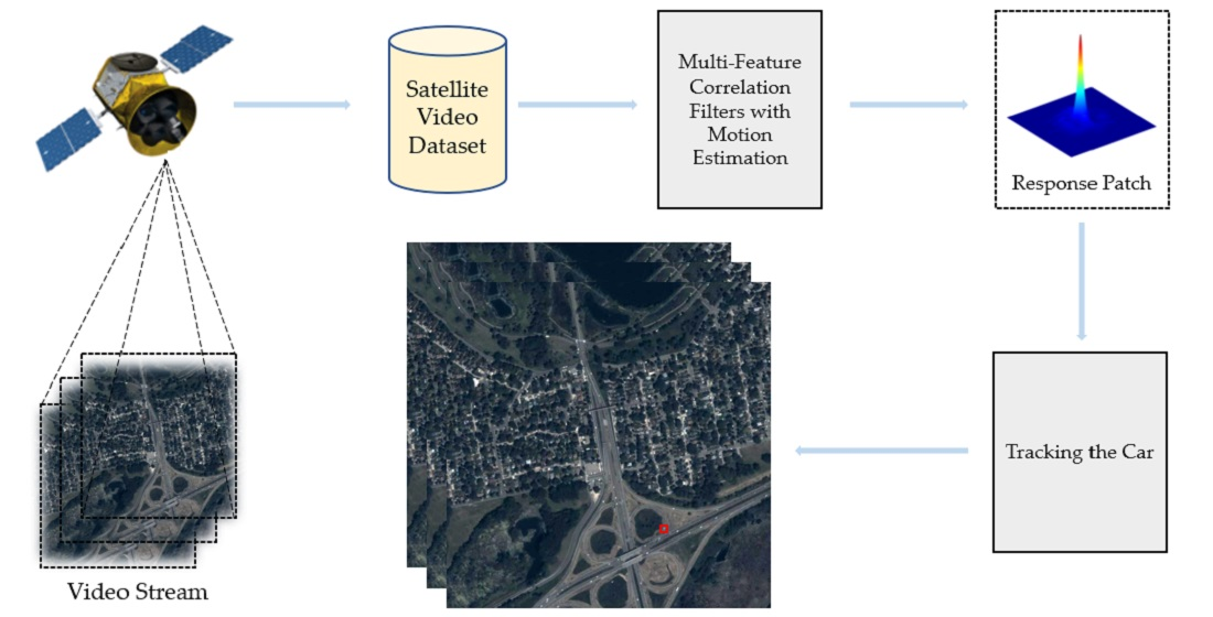
Figure 2.
Flowchart of our algorithm.

Figure 3.
Flowchart of motion estimation algorithm.

Figure 4.
Divided response patch.

Figure 5.
Tracked target is a car. (a) Car is running normally. (b) Car is occluded by overpass. (c) Car reappears after being occluded.
Figure 5.
Tracked target is a car. (a) Car is running normally. (b) Car is occluded by overpass. (c) Car reappears after being occluded.

Figure 6.
Visualisation of the tracking.

Figure 7.
Success plot on every threshold. The values in legends are the AUC.

Figure 8.
Precision plot and success plot. The values in legends are the AUC. (a) Precision plot of video1. (b) Success plot of video1. (c) Precision plot of video2. (d) Success plot of video2.
Figure 8.
Precision plot and success plot. The values in legends are the AUC. (a) Precision plot of video1. (b) Success plot of video1. (c) Precision plot of video2. (d) Success plot of video2.


Figure 9.
Precision plot and success plot. The values in legends are the AUC. (a) Precision plot of video3. (b) Success plot of video3.
Figure 9.
Precision plot and success plot. The values in legends are the AUC. (a) Precision plot of video3. (b) Success plot of video3.

Figure 10.
Precision plot and success plot. The values in legends are the AUC. (a) Precision plot of video4. (b) Success plot of video4.
Figure 10.
Precision plot and success plot. The values in legends are the AUC. (a) Precision plot of video4. (b) Success plot of video4.

Figure 11.
Precision plot and success plot. The values in legends are the AUC. (a) Precision plot of video5. (b) Success plot of video5.
Figure 11.
Precision plot and success plot. The values in legends are the AUC. (a) Precision plot of video5. (b) Success plot of video5.

Figure 12.
Visualisation of tracking results. (a) Visualisation of video1. (b) Visualisation of video2. (c) Visualisation of video3. (d) Visualisation of video4. (e) Visualisation of video5.
Figure 12.
Visualisation of tracking results. (a) Visualisation of video1. (b) Visualisation of video2. (c) Visualisation of video3. (d) Visualisation of video4. (e) Visualisation of video5.


Table 1.
Parameter values.
| Parameters | Description | Value |
|---|---|---|
| The learning rate | 0.012 | |
| The regularisation factor | 0.0001 | |
| The inertia factor | 0.075 | |
| Block number | 11 | |
| The disruptor-aware threshold | 0.47 | |
| The penalty coefficient | 3 | |
| The label function | a 2-D Gaussian function | |
| The cell of HOG | 4 × 4 | |
| The size of search area | 2.5 times the target size |
Table 2.
The detail information about the datasets.
| Videos | Target Type | Image Size | Target Size | Frame Number | Data Source |
|---|---|---|---|---|---|
| Video1 | Plane | 1450 × 750 | 30 × 30 | 180 | Jilin-1 |
| Video2 | Ship | 512 × 512 | 27 × 29 | 300 | Jilin-1 |
| Video3 | Car | 1024 × 1024 | 9 × 13 | 130 | Jilin-1 |
| Video4 | Car | 1024 × 1024 | 6 × 8 | 320 | Jilin-1 |
| Video5 | Car | 1920 × 1080 | 8 × 10 | 140 | Public data |
Table 3.
Results of video1.
| Ours | CFME | MOSSE | KCF | MIL | BOOSTING | MEDIANFLOW | |
|---|---|---|---|---|---|---|---|
| Precision Score | 0.971 | 0.956 | 0.032 | 0.928 | 0.301 | 0.852 | 0.578 |
| Success Score | 1.000 | 1.000 | 0.033 | 0.842 | 0.548 | 1.000 | 0.786 |
| AUC | 0.783 | 0.778 | 0.062 | 0.663 | 0.526 | 0.752 | 0.624 |
| FPS | 64 | 108 | 598 | 113 | 7 | 49 | 81 |
Table 4.
Results of video2.
| Ours | CFME | MOSSE | KCF | MIL | BOOSTING | MEDIANFLOW | |
|---|---|---|---|---|---|---|---|
| Precision Score | 1.000 | 1.000 | 0.163 | 0.907 | 0.608 | 0.828 | 0.376 |
| Success Score | 1.000 | 1.000 | 0.086 | 1.000 | 0.816 | 1.000 | 0.733 |
| AUC | 0.802 | 0.795 | 0.087 | 0.732 | 0.636 | 0.713 | 0.595 |
| FPS | 66 | 109 | 600 | 115 | 7 | 51 | 83 |
Table 5.
Results of video3.
| Ours | CFME | MOSSE | KCF | MIL | BOOSTING | MEDIANFLOW | |
|---|---|---|---|---|---|---|---|
| Precision Score | 0.935 | 0.920 | 0.024 | 0.521 | 0.557 | 0.578 | 0.596 |
| Success Score | 0.843 | 0.840 | 0.029 | 0.593 | 0.551 | 0.590 | 0.483 |
| AUC | 0.704 | 0.698 | 0.068 | 0.426 | 0.417 | 0.395 | 0.367 |
| FPS | 70 | 118 | 605 | 127 | 8 | 58 | 88 |
Table 6.
Results of video4.
| Ours | CFME | MOSSE | KCF | MIL | BOOSTING | MEDIANFLOW | |
|---|---|---|---|---|---|---|---|
| Precision Score | 0.969 | 0.563 | 0.114 | 0.745 | 0.664 | 0.527 | 0.515 |
| Success Score | 0.905 | 0.474 | 0.024 | 0.689 | 0.453 | 0.489 | 0.274 |
| AUC | 0.723 | 0.422 | 0.069 | 0.541 | 0.482 | 0.417 | 0.291 |
| FPS | 73 | 121 | 608 | 129 | 9 | 61 | 91 |
Table 7.
The results of video5.
| Ours | CFME | MOSSE | KCF | MIL | BOOSTING | MEDIANFLOW | |
|---|---|---|---|---|---|---|---|
| Precision Score | 0.974 | 0.952 | 0.124 | 0.754 | 0.921 | 0.700 | 0.855 |
| Success Score | 0.821 | 0.802 | 0.056 | 0.596 | 0.450 | 0.132 | 0.334 |
| AUC | 0.703 | 0.698 | 0.083 | 0.461 | 0.519 | 0.288 | 0.421 |
| FPS | 71 | 118 | 606 | 127 | 8 | 59 | 89 |
Table 8.
Results of ablation experiment.
| Baseline | +M1 | +M1+M2 | +M1+M2+M3 | |
|---|---|---|---|---|
| Precision Score | 0.771 | 0.933 | 0.951 | 0.969 |
| Success Score | 0.744 | 0.891 | 0.906 | 0.914 |
| AUC | 0.565 | 0.722 | 0.736 | 0.743 |
| FPS | 122 | 107 | 86 | 69 |
Publisher’s Note: MDPI stays neutral with regard to jurisdictional claims in published maps and institutional affiliations. |
© 2022 by the authors. Licensee MDPI, Basel, Switzerland. This article is an open access article distributed under the terms and conditions of the Creative Commons Attribution (CC BY) license (https://creativecommons.org/licenses/by/4.0/).
Share and Cite
MDPI and ACS Style
Zhang, Y.; Chen, D.; Zheng, Y. Satellite Video Tracking by Multi-Feature Correlation Filters with Motion Estimation. Remote Sens. 2022, 14, 2691. https://doi.org/10.3390/rs14112691
AMA Style
Zhang Y, Chen D, Zheng Y. Satellite Video Tracking by Multi-Feature Correlation Filters with Motion Estimation. Remote Sensing. 2022; 14(11):2691. https://doi.org/10.3390/rs14112691
Chicago/Turabian StyleZhang, Yan, Deng Chen, and Yuhui Zheng. 2022. "Satellite Video Tracking by Multi-Feature Correlation Filters with Motion Estimation" Remote Sensing 14, no. 11: 2691. https://doi.org/10.3390/rs14112691
Note that from the first issue of 2016, this journal uses article numbers instead of page numbers. See further details here.