
Semantic Segmentation of Multispectral Images via Linear Compression of Bands: An Experiment Using RIT-18


Department of Civil Engineering, Xi’an Jiaotong-Liverpool University, Suzhou 215123, China
*
Author to whom correspondence should be addressed.
Remote Sens. 2022, 14(11), 2673; https://doi.org/10.3390/rs14112673
Submission received: 18 April 2022
/
Revised: 18 May 2022
/
Accepted: 30 May 2022
/
Published: 2 June 2022
(This article belongs to the Special Issue Optical Remote Sensing Applications in Urban Areas II)
Abstract
:Semantic segmentation of remotely sensed imagery is a basic task for many applications, such as forest monitoring, cloud detection, and land-use planning. Many state-of-the-art networks used for this task are based on RGB image datasets and, as such, prefer three-band images as their input data. However, many remotely sensed images contain more than three spectral bands. Although it is technically possible to feed multispectral images directly to those networks, poor segmentation accuracy was often obtained. To overcome this issue, the current image dimension reduction methods are either to use feature extraction or to select an optimal combination of three bands through different trial processes. However, it is well understood that the former is often comparatively less effective, because it is not optimized towards segmentation accuracy, while the latter is less efficient due to repeated trial selections of three bands for the optimal combination. Therefore, it is meaningful to explore alternative methods that can utilize multiple spectral bands efficiently in the state-of-the-art networks for semantic segmentation of similar accuracy as the trial selection approach. In this study, a hot-swappable stem structure (LC-Net) is proposed to linearly compress the input bands to fit the input preference of typical networks. For the three commonly used network structures tested on the RIT-18 dataset (having six spectral bands), the approach proposed was found to be an equivalently effective but much more efficient alternative to the trial selection approach.
1. Introduction
Semantic segmentation of images is a fundamental task in computer vision, in which a label is assigned to each pixel. For remotely sensed imagery, its semantic segmentation (known as pixel-based classification previously) is the basis for many applications, such as forest monitoring, cloud detection, and land-use planning [1,2,3,4]. There are sensors that can capture images with more than three bands (e.g., multispectral and hyperspectral images). Compared to the three bands obtained by RGB cameras, the additional spectral information of multispectral images could be used to, potentially, achieve a higher segmentation accuracy. However, semantic segmentation of multispectral images is challenging due to the limited training samples and high-dimensional features.
Compared to RGB sensors with fixed spectral bands, the spectral bands between different multispectral sensors are usually different. This means that the multispectral image datasets obtained by different multispectral sensors are unique. Coupled with the fact that data annotation is very time-consuming, the total amount of annotated data available for a specific multispectral semantic segmentation task is typically very limited. Therefore, relative lightweight networks [5,6,7,8,9] were often used for multispectral semantic segmentation to avoid overfitting. However, it is a consensus that deeper and wider neural networks that have been pre-trained on large-scale datasets can achieve a higher segmentation accuracy compared to lighter neural networks without pre-training. Many neural networks developed for RGB images have become deeper and wider and achieved excellent performances on many challenging benchmark datasets. Hence, the accuracy of multispectral semantic segmentation may be improved significantly if the multispectral images can be tailored properly to fit the pre-trained state-of-the-art networks. Due to the peak phenomenon [10,11,12], direct feeding of multispectral images to networks developed originally for three-channel images often leads to poor segmentation accuracy [13,14,15]. The most direct solution to this problem is to reduce the input image dimension to three.
There are mainly two types of methods for image dimensionality reduction, i.e., feature extraction [16,17,18,19,20,21,22,23] and band selection [15,24,25,26,27,28,29]. The representative feature extraction methods include principle component analysis-based methods [20,22,30,31,32], independent component analysis-based methods [16], linear discriminant analysis-based methods [17,33,34], and locality preserving projection-based methods [35,36]. Most of these methods perform linear transformations of the original spectral bands to optimize their objectives. One common objective in the feature extraction methods is to retain as much information as possible in the processed images (in which the dimension is reduced). Existing feature extraction methods are generally fast in processing, but the changes in the original spectral reflectance may cause difficulties in physical interpretations and hinder the applications where physical spectral measurements are required. In addition, since the optimization objectives of those methods are not on the segmentation accuracy of the neural networks, they do not guarantee a decent performance in segmentation.
Band selection refers to the selection of a subset of spectrum bands from the original image. Depending on the usage of labeled images during the selection process, band selection can be categorized as unsupervised [37,38,39,40,41,42,43] and supervised [44,45,46,47,48,49,50,51] methods. The former one is to select the most representative bands based on their statistical characteristics, such as dissimilarity, information entropy, information divergence, or correlation. The latter one typically uses the labeled images to select a band combination that maximizes class separability. In general, the band selection methods require an iterative trial of band combinations, which is more computationally intensive than the feature extraction methods. As for the advantages, unsupervised band selection methods are more popular among scholars as they do not require labeled data and have more application scenarios. Meanwhile, the supervised band selection methods have been proven to achieve a better segmentation accuracy than other types of existing methods.
Motived by the aforementioned limitations of the current methods and inspired initially by the fact that adjacent bands of the multispectral/hyperspectral images are usually relatively similar, a hot-pluggable head structure for the linear compression (referred to as LC-Net) of bands is proposed in this study for a supervised feature extraction, which directly optimizes the segmentation accuracy. The main advantages of LC-Net are its compatibility with existing networks and faster training speed while maintaining similar accuracy compared to the supervised grid search (SGS). The structure of LC-Net can be kept as simple as possible, which adds negligible computational costs to the training and inference processes. The effectiveness of LC-Net was tested using three different networks on the RIT-18 benchmark dataset [5] in this study.
2. Materials and Methods
2.1. Study Data
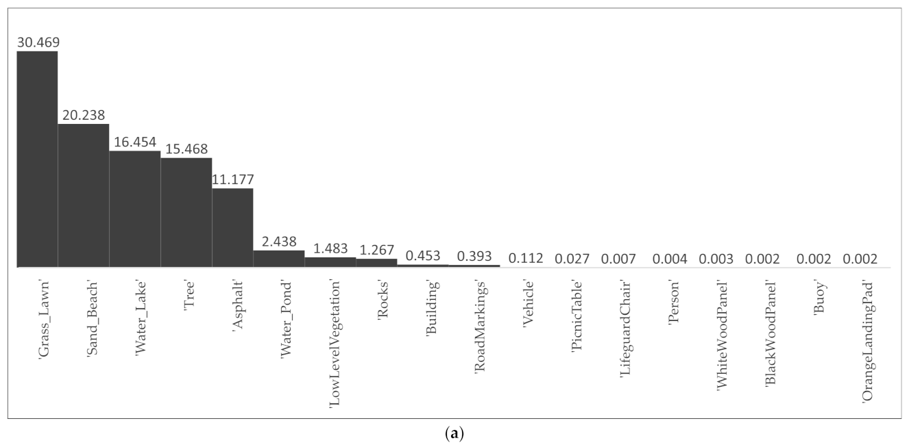
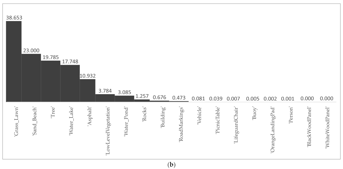
The RIT-18 [5] multispectral dataset used in this study is a six-band multispectral dataset that includes visible RGB bands (band 3 for R, band 2 for G, and band 1 for B) and three near-infrared bands (bands 4–6). It contains a training image with a resolution of 9393 × 5642 and a test image with a resolution of 8833 × 6918. Each pixel of the images in RIT-18 is assigned to one of the eighteen classes. A comparison between RIT-18 and other commonly used publicly available multispectral datasets is summarized in Table 1. It shows that RIT-18 has the largest number of labeled classes and the finest ground sample distance (GSD) compared to ISPRS Vaihingen and Potsdam [52], Zurich Summer [53], and L8 SPARCS [54]. Together with the highly unbalanced classes, as shown in Figure 1, they make RIT-18 a very challenging dataset. In addition, as a 6-band dataset, RIT-18 has a total of 20 combinations of three bands, which is neither too many (120 possible combinations), as in L8 SPARCS, nor too few, as in other datasets. Therefore, as a challenging but computationally affordable dataset, RIT-18 was considered in this study.
To avoid any confusion, it is worth mentioning that there are 18 classes in the training images but only 16 classes in the test images, which explains why 16 classes are shown in the subsequent sections.
2.2. LC-Net
Despite the rich spectral information contained in the multispectral images, these additional bands cause new challenges, not only in terms of more GPU memory and computational consumption but also in the peak phenomenon [10,11,12]. This phenomenon shows that the use of additional features (e.g., spectral bands) introduces complexity to the classifier and increases the number of parameters and training data needed to achieve the same classification accuracy (using fewer features). Directly using more features may lead to worse classification results [12,55]. To address this problem, LC-Net is proposed in this study to reduce the number of input channels for the subsequent network at the initial stage. This prevents the subsequent network from receiving too many features while allowing the network to choose its preferred features.
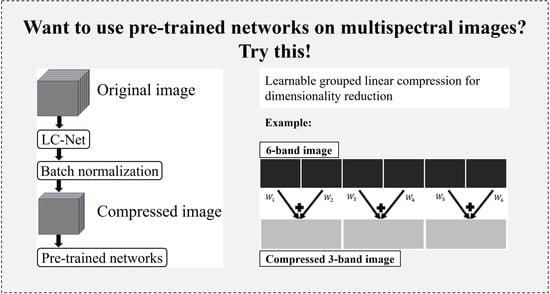
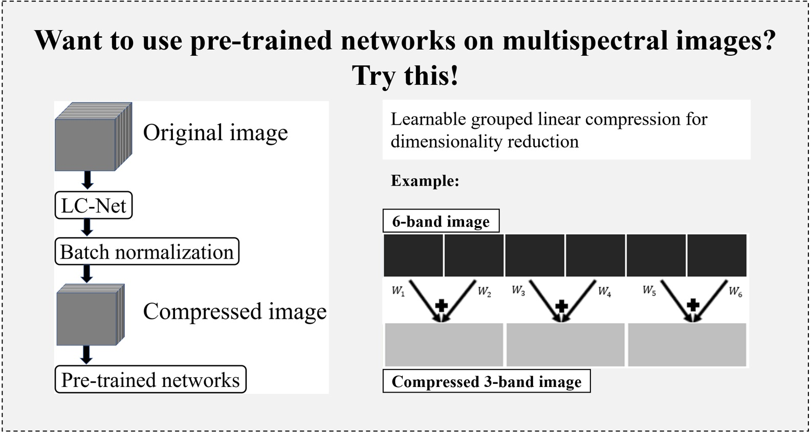
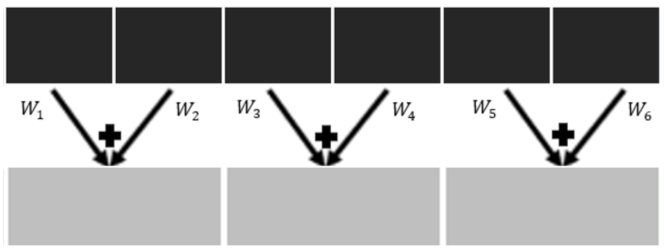
The LC-Net is defined as a 1 × 1 group convolution layer with 2 bands per group at the initial stage of the networks. This setup will compress two adjacent input bands in sequence without any overlap, as shown in Figure 2. More specifically, each band was multiplied by a weight, and, after that, two adjacent bands (i.e., bands 1 and 2, bands 3 and 4, and bands 5 and 6 for the RIT-18 dataset) were added together to form three new bands. The weights applied to the bands were randomly initialized and iteratively updated during the training.
In addition, for a more comprehensive understanding, the performance of combining non-adjacent bands was also tested. The implementation details are shown in Section 2.5. Unless stated otherwise, the LC-Net referred to in the following sections is based on the combination of adjacent bands.
Most of the multispectral datasets listed in Table 1 have even bands, although multispectral sensors with odd bands do exist. For cases where the number of original bands is not adequate to form three post-compression bands, blank bands may be added to the original bands to be compatible with LC-Net. As adding a blank band does not provide any new features to the model, it does not introduce additional complexity to the classifier and, thus, does not suffer from the peaking phenomenon.
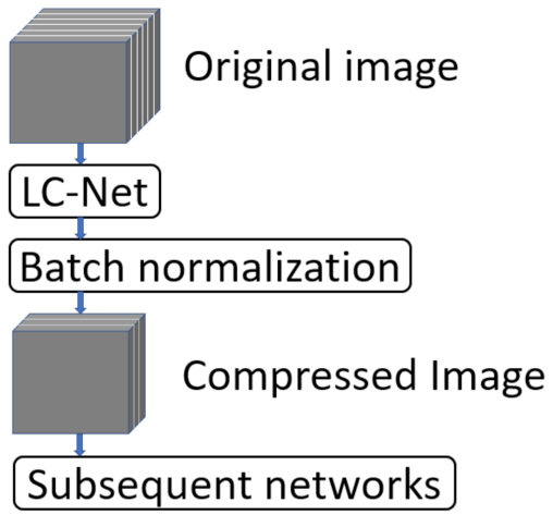
As shown in Figure 3, the feature maps obtained from LC-Net can be fed to any existing networks for subsequent processing after passing through a batch normalization layer. There is no non-linear activation layer used after the batch normalization layer, not only because it is not consistent with the linear compression that LC-Net aims to achieve but also because the application of activation functions to low-dimensional features (3 dimensions in this case) can degrade network performance, as demonstrated by many studies [56,57,58].
The subsequent networks shown in Figure 3 include an encoder and a decoder. For the encoder (i.e., backbone), the networks used in this study consist of ResNet50 [59], HRNet-w18 [60], and Swin-tiny [61], which are popular convolutional neural networks and vision transformers. All the backbones are pre-trained using the ImageNet dataset [62]. For the decoder, the same decoder structure of Fully Convolutional Networks (FCN) [63] is used for all the networks adopted in this study. The detailed network structures faithfully follow their original implementations and are described in detail in Section 2.3.
2.3. Network Structure
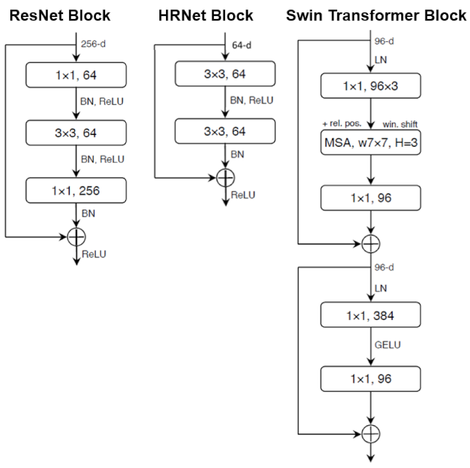
The backbones (i.e., ResNet [59], HRNet [60], and Swin [61]) used in this study can be considered three milestones in the network’s structure design. For example, the residual connection proposed by ResNet [59] has become a standard paradigm for subsequent network designs. The basic block design of ResNet [59] is shown in Figure 4, which consists of a stack of convolution layers, a Batch Normalization (BN) layer, and a Rectified Linear Unit (ReLU). The complete ResNet [59] is constructed by connecting the stem and the multiple basic blocks in a series. The detailed architecture specifications of ResNet-50 are presented in Table 2. The overall design follows two rules: One is to apply the same hyperparameters (the width and filter size) to the blocks of the same spatial resolution. The other is that when the spatial resolution is reduced by half, the width of the block doubles. The second rule ensures that all blocks have approximately the same computational complexity in terms of floating-point operations (FLOPs). Similar to residual connection, these two rules were applied to most network designs, including Swin [61] and HRNet [60].
As shown in Table 2, the macro design of Swin [61] is similar to that of ResNet [59]. Both are single-branch structures. As the network depth increases, the spatial resolution gradually decreases, and the width increases. Their main differences are within the basic blocks, as shown in Figure 4 and Table 2. The basic block of Swin is built by a Multi-head Self-Attention (MSA) module with shifted windows (win. shift) and relative position bias (rel. pos), followed by a two Multi-Layer Perceptron (MLP) with a Gaussian Error Linear Unit (GELU) in between. For clarity, the MLP layers in Swin [61] are noted as a “1 × 1 convolution” in Figure 4 since they are equivalent.
The main innovation of HRNet [60] is the use of four parallel branches of the same depth, corresponding to four down-sampling levels (4, 8, 16, and 32). Compared to single-branch backbones, HRNet [60] significantly increases the network depth with respect to fine-resolution features. This proves to be beneficial for pixel-level image processing tasks [64,65,66]. The basic block and detailed architecture specifications of HRNet-w18 are shown in Figure 4 and Table 3, respectively.
2.4. Training Setting
The experiment was carried out on a PC with a processor of AMD Ryzen 9 3950X, RAM of 64 GB, and two GPUs of NVIDIA GeForce GTX 3090. In addition, the PyTorch framework [67] in Ubuntu (20.04) was used for programming the experiment. For a fair comparison of the whole experiment process, all the trainings used the same training protocol, which is a strategy used widely in the research of deep learning [61,68,69]. More specifically, the AdamW optimizer was adopted with the following setup: a base learning rate of 0.00006, a weight decay of 0.01, a linear learning rate decay, and a linear warmup of 1500 iterations.
For the data augmentation, the images with a size of 512 × 512 were extracted randomly, in addition to the application of a random horizontal and vertical flipping. Due to the limited physical memory of our GPU cards, the batch size was set to be 16, and synchronized batch normalization across the GPU cards was adopted during the training. The total number of training iterations was 15,000. Similar to [60,70,71], by applying the random data augmentation and the batch normalization, all the networks used in this study are considered resistant to overfitting.
2.5. Comparisons
To check the performance (i.e., segmentation accuracy and efficiency) of using LC-Net, our approach was compared with three commonly used approaches.
The first one is the Direct Feeding (DF) approach, which is to modify the first convolutional layer (typically 3 kernel channels) in the networks (i.e., ResNet50, HRNet-w18, and Swin-tiny) so that the number of kernel channels is identical to the number of bands of the input image. In the case of RIT-18 (6 bands), the modified first convolutional layer has 6 kernel channels, the initial parameters of which are randomly allocated.
The second approach is Principal Component Analysis (PCA). More specifically, the singular value decomposition method is adopted for extracting the first three principal components. The extracted 3-band images are used as the network input.
The third approach is a Supervised Grid Search (SGS), in which the optimal combination of the 3-band is determined by trialing all possible combinations. As the most fundamental band selection method, it ensures the selection of the optimal band combination. To facilitate fairer comparisons between those approaches, the parameters in the first convolutional layer of the pre-trained backbones were randomly reset in the DF approach, the SGS approach, and the LC-Net approach.
Further to the aforementioned three approaches, two alternative means of band compressions are also investigated in this study, which is detailed in the next two paragraphs.
The band compression using two adjacent bands (i.e., Figure 2) in LC-Net is based on the assumption that the neighboring bands are often more similar to each other and, therefore, less effective information may be lost in this way. To test whether this hypothesis is necessary, a compression of non-adjacent bands (e.g., bands 1 and 3, bands 2 and 5, and bands 4 and 6) in the same means was also tested to explore the differences.
In addition to the compressions of two bands into one to form a 3-band image using RIT-18, another test is considered, in which all bands are compressed to form each band of the 3-band input image (i.e., all bands are compressed three times, and a new band is produced each time). This is referred to as the Linear Combination of All Bands (LCAB). Since the number of output bands is not constrained by the number of input bands, the LCAB approach is more flexible than LC-Net. However, since each band of the output image is a linear combination of all input bands, LCAB potentially suffers from a greater influence of the mixed spectral information received.
3. Results
The results of the PCA, DF, and LC-Net approaches are summarized in Table 4. The segmentation accuracy using the PCA approach was considerably lower than those of the other two approaches and, therefore, was not analyzed in detail. It was observed that the use of LC-Net brought consistent improvements in the final segmentation performance. In comparison to those using the DF approach, an average improvement of 12.1% in overall accuracy (OA) was achieved by adding LC-Net. Meanwhile, for the more critical accuracy metric, i.e., the mean accuracy (MA), the use of LC-Net led to an average improvement of 14.0% compared to those obtained using the DF approach. The processing time introduced by the extra learnable parameters (six weights in these cases) was found to be negligible. It is worth mentioning that the best semantic segmentation results obtained in this study (i.e., Swin-tiny+ LC-Net) outperformed the traditional machine learning and deep learning approaches reported in the literature [9,72,73]. For example, the best results (those fine-tuned without additional data) so far on RIT-18 were achieved by CoinNet [73], which were exceeded by 2.2% and 8.0% in terms of OA and MA, respectively, using our approach.
To check the effectiveness of the results using LC-Net, the accuracy of the segmentation results using a trial selection of all possible combinations (20 in total) of the three bands was also investigated in this study. Table 5 shows the segmentation accuracies of the networks used with different combinations of the three input bands. It was observed that the accuracies achieved under each combination varied. For the three networks considered, the accuracy of the most accurate combination was on average 1.30% lower and 1.07% lower than those of LC-Net for the OA metric and the MA metric, respectively. In addition to this, LC-Net requires much less time than the band selection method because it only needs to be trained once. A visual comparison between DF, SGS, and LC-Net for Swin-tiny is shown in Figure 5. It is observed that the results of DF are notably worse than the other two methods.
The aforementioned results are based on a particular compression of two adjacent bands into one (i.e., one from bands 1 and 2, one from bands 3 and 4, and one from bands 5 and 6). No adjacent bands were also considered for the band compression. Table 6 shows the comparisons between the performances of LC-Net using adjacent bands or non-adjacent bands. Very small differences were observed in the overall accuracies. In addition, the segmentation accuracies of LCAB are shown for comparison to LC-Net in Table 6. Significant degradation in the segmentation accuracy was observed.
4. Discussion
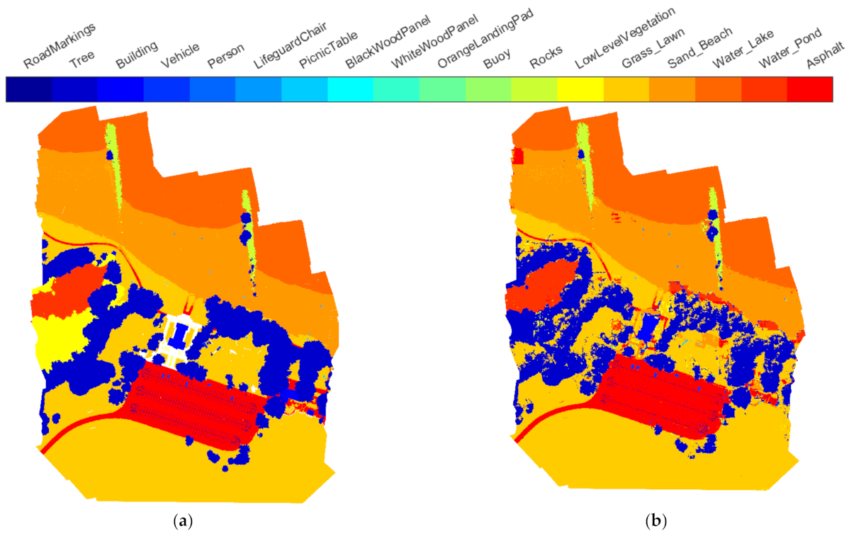
The segmentation results of ResNet50+ LC-Net, HRNet-w18+ LC-Net, and Swin-tiny+ LC-Net are shown in Figure 6. Compared to the ground truth (Figure 6a), it was seen that the majority of the pixels were correctly labeled using any of those networks. To understand the likely causes for the mislabeled pixels by the networks, the spectral information (i.e., the RGB images of bands 1–3 and the pseudo color images of bands 4–6) of RIT-18 is shown in Figure 7. After the visual comparisons between Figure 6 and Figure 7, it was found that segmentation errors appeared mainly in three types of areas: the object edges, shaded areas, and changes in terrain. In contrast to extensive attention received in the field of semantic segmentation [4,74] for improving the segmentation accuracy at the object edges, the latter two error sources have not received much attention. To address these issues, it is necessary to identify the causes of the segmentation errors in those regions. A relatively large mislabeled local area was marked with a black dashed box in both Figure 6 and Figure 7, where a continuous area of low-level vegetation was segmented as other classes (mainly tree or grass/lawn). As shown in Figure 7, the area is a valley where the surrounding trees cast shadows, which resulted in abrupt changes in the spectral characteristics of the low-level vegetation. Another common reason worth considering for the low segmentation accuracy of a particular class in the test set is the under-representation of that class in the training set. For RIT-18, the proportion of low-level vegetation in the training data ranks seventh among all classes. The eighth, ninth, and tenth classes in the training data are rocks, buildings, and road signs, with 1.27%, 0.45%, and 0.39%, respectively. Their segmentation accuracy (Swin-tiny + LC-Net) on the test set was 90.3%, 65.0%, and 63.1%, respectively, which all are much higher than that of low-level vegetation. Therefore, the lack of training data may not be the reason for the low segmentation accuracy of low-level vegetation, and the abrupt changes in the spectral characteristics are likely to be the cause of the mis-segmentation. Similarly, the shadows of trees on the sandy beach surface seemed to cause a mix of mislabeled pixels as enveloped by a solid purple box. Therefore, future studies may consider pre-identifying areas with shadows and topographic changes and treating them separately. This may require additional labeling of such areas or additional data, such as digital elevation models and solar information about the target area.
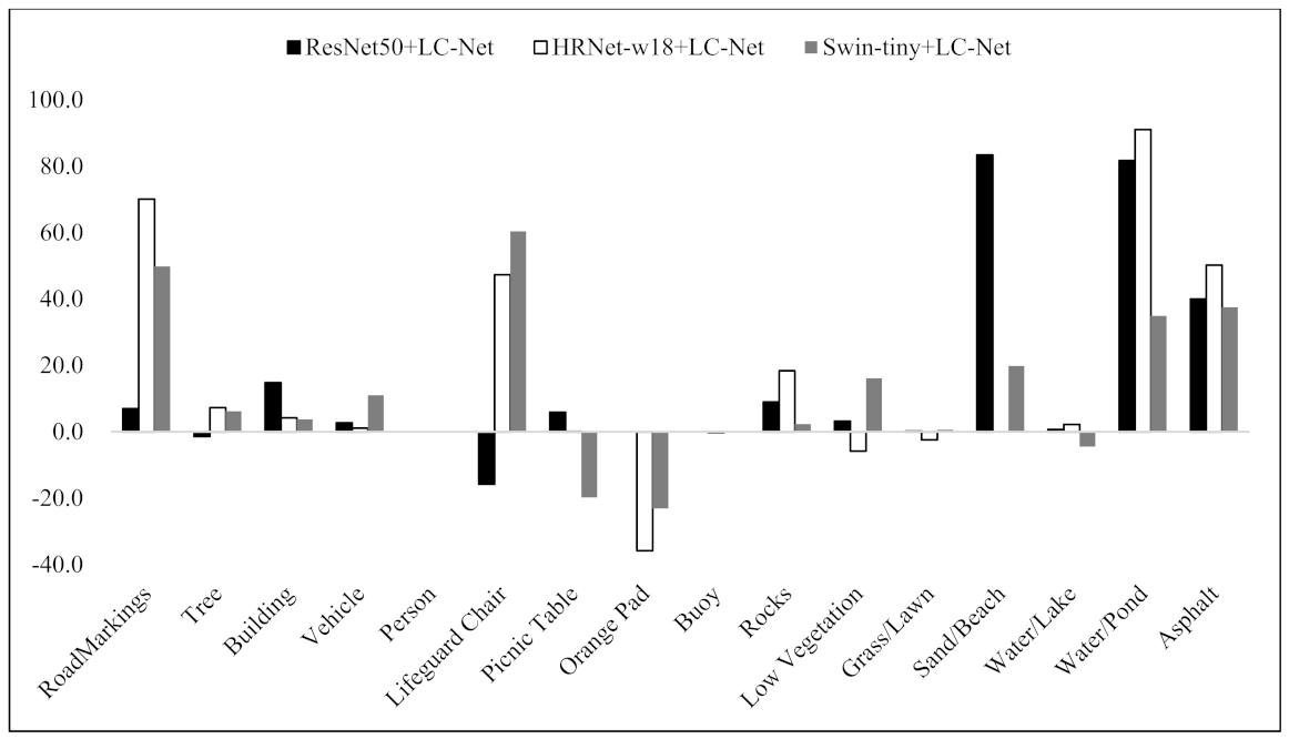
While the results demonstrate that adding LC-Net to the networks can improve the overall segmentation performance, not every segmented class can benefit from LC-Net, as shown in Figure 8. The likely reason for this is that LC-Net forces the neural networks to perform a relative aggressive band compression in the initial stage, which inevitably causes a certain amount of information loss. Since the weights of LC-Net were randomly initialized and the weights in the backbone were also different, the lost information may, by chance, include the one that is important for a specific class. This conjecture can be inferred to some extent by the information in Table 7, where the final weights of LC-Net associated with the three network structures were recorded and show no specific pattern. Therefore, future studies may focus on finding more effective band compression methods. For example, more complex (e.g., a 3 × 3 convolutional kernel), nonlinear (e.g., adding the activation function after the LC-Net), and multilayer band compression methods might be able to compress more effective information into the same number of bands.
LC-Net compresses the number of bands in RIT-18 to half of its original number. However, the optimal level of the band compression (with respect to the number of bands) may not be exactly half of the original number. As such, future research may focus on how to set the degree of the band compression as a learnable variable to improve the network performance further.
5. Conclusions
Neural networks have been proven to be powerful tools for semantic segmentation with respect to RGB images. However, the application of those networks to multispectral images that have many more bands usually requires a tedious and time-consuming trial band selection process. To solve this problem, a simple LC-Net is proposed in this study to automatically reduce the number of bands to fit that required by networks via an embedded learning process at almost no cost. It was found that the accuracies (in terms of OA and MA) of the semantic segmentation on RIT-18 were significantly improved (12.1% and 14.03%, respectively) when LC-Net was added to the networks considered. In comparison to the SGS of the optimal combination of three bands (from 20 possible combinations for RIT-18), the segmentation accuracies using LC-Net were found to be slightly higher than those of the optimal combination of three bands obtained through the time-consuming exhaustive selection. Meanwhile, the computational cost of LC-Net was much less than the trial selection process.
Author Contributions
Conceptualization, Y.C. and L.F.; formal analysis, Y.C.; funding acquisition, L.F.; investigation, Y.C., L.F. and C.Z.; methodology, Y.C. and L.F.; supervision, L.F.; writing—original draft, Y.C.; writing—review and editing, L.F. and C.Z. All authors have read and agreed to the published version of the manuscript.
Funding
This research was funded by the Xi’an Jiaotong-Liverpool University Research Enhancement Fund (grant number REF-21-01-003), Xi’an Jiaotong-Liverpool University Key Program Special Fund (grant number KSF-E-40), and Xi’an Jiaotong-Liverpool University Research Development Fund (grant number RDF-18-01-40).
Data Availability Statement
The data presented in this study are openly available in [http://www.cis.rit.edu/~rmk6217/rit18_data.mat, accessed on 5 May 2021] at [https://doi.org/10.1016/j.isprsjprs.2018.04.014], reference number [5].
Conflicts of Interest
The authors declare no conflict of interest.
References
- Dechesne, C.; Mallet, C.; Le Bris, A.; Gouet-Brunet, V. Semantic Segmentation of Forest Stands of Pure Species as a Global Optimization Problem. In Proceedings of the ISPRS Annals of the Photogrammetry, Remote Sensing and Spatial Information Sciences, Hannover, Germany, 6–9 June 2017; Volume 4, pp. 141–148. [Google Scholar]
- Dong, Z.; Yang, B.; Hu, P.; Scherer, S. An efficient global energy optimization approach for robust 3D plane segmentation of point clouds. ISPRS J. Photogramm. Remote Sens. 2018, 137, 112–133. [Google Scholar] [CrossRef]
- Goldblatt, R.; Stuhlmacher, M.F.; Tellman, B.; Clinton, N.; Hanson, G.; Georgescu, M.; Wang, C.; Serrano-Candela, F.; Khandelwal, A.K.; Cheng, W.H.; et al. Using Landsat and nighttime lights for supervised pixel-based image classification of urban land cover. Remote Sens. Environ. 2018, 205, 253–275. [Google Scholar] [CrossRef]
- Marmanis, D.; Schindler, K.; Wegner, J.D.; Galliani, S.; Datcu, M.; Stilla, U. Classification with an edge: Improving semantic image segmentation with boundary detection. ISPRS J. Photogramm. Remote Sens. 2018, 135, 158–172. [Google Scholar] [CrossRef] [Green Version]
- Kemker, R.; Salvaggio, C.; Kanan, C. Algorithms for semantic segmentation of multispectral remote sensing imagery using deep learning. ISPRS J. Photogramm. Remote Sens. 2018, 145, 60–77. [Google Scholar] [CrossRef] [Green Version]
- Lawin, F.J.; Danelljan, M.; Tosteberg, P.; Bhat, G.; Khan, F.S.; Felsberg, M. Deep projective 3D semantic segmentation. In Proceedings of the International Conference on Computer Analysis of Images and Patterns, Ystad, Sweden, 22–24 August 2017; Lecture Notes in Computer Science (Including Subseries Lecture Notes in Artificial Intelligence and Lecture Notes in Bioinformatics). Springer: Cham, Switherland, 2017; Volume 10424 LNCS, pp. 95–107. [Google Scholar]
- Mateo-García, G.; Laparra, V.; López-Puigdollers, D.; Gómez-Chova, L. Transferring deep learning models for cloud detection between Landsat-8 and Proba-V. ISPRS J. Photogramm. Remote Sens. 2020, 160, 1–17. [Google Scholar] [CrossRef]
- Boulch, A.; Guerry, J.; Le Saux, B.; Audebert, N. SnapNet: 3D point cloud semantic labeling with 2D deep segmentation networks. Comput. Graph. 2018, 71, 189–198. [Google Scholar] [CrossRef]
- Saxena, N.; Babu, N.K.; Raman, B. Semantic segmentation of multispectral images using res-seg-net model. In Proceedings of the Proceedings—14th IEEE International Conference on Semantic Computing, ICSC 2020, San Diego, CA, USA, 5 October 2019; Institute of Electrical and Electronics Engineers Inc.: New York, NY, USA, 2020; pp. 154–157. [Google Scholar]
- Sima, C.; Dougherty, E.R. The peaking phenomenon in the presence of feature-selection. Pattern Recognit. Lett. 2008, 29, 1667–1674. [Google Scholar] [CrossRef]
- Kallepalli, A.; Kumar, A.; Khoshelham, K. Entropy based determination of optimal principal components of Airborne Prism EXperiment (APEX) imaging spectrometer data for improved land cover classification. In Proceedings of the International Archives of the Photogrammetry, Remote Sensing and Spatial Information Sciences—ISPRS Archives, Hyderabad, India, 9–12 December 2014; International Society for Photogrammetry and Remote Sensing: Hannover, Germany, 2014; Volume 40, pp. 781–786. [Google Scholar]
- Theodoridis, S.; Koutroumbas, K. Pattern recognition and neural networks. In Proceedings of the Lecture Notes in Computer Science (Including Subseries Lecture Notes in Artificial Intelligence and Lecture Notes in Bioinformatics); Springer: Berlin/Heidelberg, Germany, 2001; Volume 2049 LNAI, pp. 169–195. [Google Scholar]
- Cai, Y.; Fan, L.; Atkinson, P.M.; Zhang, C. Semantic Segmentation of Terrestrial Laser Scanning Point Clouds Using Locally Enhanced Image-Based Geometric Representations. IEEE Trans. Geosci. Remote Sens. 2022, 60, 1–15. [Google Scholar] [CrossRef]
- Cai, Y.; Huang, H.; Wang, K.; Zhang, C.; Fan, L.; Guo, F. Selecting Optimal Combination of Data Channels for Semantic Segmentation in City Information Modelling (CIM). Remote Sens. 2021, 13, 1367. [Google Scholar] [CrossRef]
- Bhuiyan, M.A.E.; Witharana, C.; Liljedahl, A.K.; Jones, B.M.; Daanen, R.; Epstein, H.E.; Kent, K.; Griffin, C.G.; Agnew, A. Understanding the effects of optimal combination of spectral bands on deep learning model predictions: A case study based on permafrost tundra landform mapping using high resolution multispectral satellite imagery. J. Imaging 2020, 6, 97. [Google Scholar] [CrossRef]
- Wang, J.; Chang, C.I. Independent component analysis-based dimensionality reduction with applications in hyperspectral image analysis. IEEE Trans. Geosci. Remote Sens. 2006, 44, 1586–1600. [Google Scholar] [CrossRef]
- Bandos, T.V.; Bruzzone, L.; Camps-Valls, G. Classification of hyperspectral images with regularized linear discriminant analysis. IEEE Trans. Geosci. Remote Sens. 2009, 47, 862–873. [Google Scholar] [CrossRef]
- Belkin, M.; Niyogi, P. Laplacian eigenmaps for dimensionality reduction and data representation. Neural Comput. 2003, 15, 1373–1396. [Google Scholar] [CrossRef] [Green Version]
- Roweis, S.T.; Saul, L.K. Nonlinear dimensionality reduction by locally linear embedding. Science 2000, 290, 2323–2326. [Google Scholar] [CrossRef] [PubMed] [Green Version]
- Farrell, M.D.; Mersereau, R.M. On the impact of PCA dimension reduction for hyperspectral detection of difficult targets. IEEE Geosci. Remote Sens. Lett. 2005, 2, 192–195. [Google Scholar] [CrossRef]
- Bhatti, U.A.; Yu, Z.; Chanussot, J.; Zeeshan, Z.; Yuan, L.; Luo, W.; Nawaz, S.A.; Bhatti, M.A.; ul Ain, Q.; Mehmood, A. Local Similarity-Based Spatial-Spectral Fusion Hyperspectral Image Classification With Deep CNN and Gabor Filtering. IEEE Trans. Geosci. Remote Sens. 2021, 60, 5514215. [Google Scholar] [CrossRef]
- Fauvel, M.; Chanussot, J.; Benediktsson, J.A. Kernel principal component analysis for the classification of hyperspectral remote sensing data over urban areas. EURASIP J. Adv. Signal Process. 2009, 2009, 783194. [Google Scholar] [CrossRef] [Green Version]
- Tenenbaum, J.B.; De Silva, V.; Langford, J.C. A global geometric framework for nonlinear dimensionality reduction. Science 2000, 290, 2319–2323. [Google Scholar] [CrossRef]
- Zhu, M.; Jiao, L.; Liu, F.; Yang, S.; Wang, J. Residual Spectral-Spatial Attention Network for Hyperspectral Image Classification. IEEE Trans. Geosci. Remote Sens. 2021, 59, 449–462. [Google Scholar] [CrossRef]
- Roy, S.K.; Manna, S.; Song, T.; Bruzzone, L. Attention-Based Adaptive Spectral-Spatial Kernel ResNet for Hyperspectral Image Classification. IEEE Trans. Geosci. Remote Sens. 2021, 59, 7831–7843. [Google Scholar] [CrossRef]
- Sun, W.; Yang, G.; Peng, J.; Meng, X.; He, K.; Li, W.; Li, H.C.; Du, Q. A Multiscale Spectral Features Graph Fusion Method for Hyperspectral Band Selection. IEEE Trans. Geosci. Remote Sens. 2021, 60, 5513712. [Google Scholar] [CrossRef]
- Su, H.; Yang, H.; Du, Q.; Sheng, Y. Semisupervised band clustering for dimensionality reduction of hyperspectral imagery. IEEE Geosci. Remote Sens. Lett. 2011, 8, 1135–1139. [Google Scholar] [CrossRef]
- Sun, W.; Peng, J.; Yang, G.; Du, Q. Correntropy-Based Sparse Spectral Clustering for Hyperspectral Band Selection. IEEE Geosci. Remote Sens. Lett. 2020, 17, 484–488. [Google Scholar] [CrossRef]
- Hu, P.; Liu, X.; Cai, Y.; Cai, Z. Band Selection of Hyperspectral Images Using Multiobjective Optimization-Based Sparse Self-Representation. IEEE Geosci. Remote Sens. Lett. 2019, 16, 452–456. [Google Scholar] [CrossRef]
- Jia, X.; Richards, J.A. Segmented principal components transformation for efficient hyperspectral remote-sensing image display and classification. IEEE Trans. Geosci. Remote Sens. 1999, 37, 538–542. [Google Scholar] [CrossRef] [Green Version]
- Zabalza, J.; Ren, J.; Yang, M.; Zhang, Y.; Wang, J.; Marshall, S.; Han, J. Novel Folded-PCA for improved feature extraction and data reduction with hyperspectral imaging and SAR in remote sensing. ISPRS J. Photogramm. Remote Sens. 2014, 93, 112–122. [Google Scholar] [CrossRef] [Green Version]
- Uddin, M.P.; Al Mamun, M.; Hossain, M.A. PCA-based Feature Reduction for Hyperspectral Remote Sensing Image Classification. IETE Tech. Rev. 2021, 38, 377–396. [Google Scholar] [CrossRef]
- Du, Q. Modified Fisher’s linear discriminant analysis for hyperspectral imagery. IEEE Geosci. Remote Sens. Lett. 2007, 4, 503–507. [Google Scholar] [CrossRef]
- Wang, Q.; Meng, Z.; Li, X. Locality Adaptive Discriminant Analysis for Spectral-Spatial Classification of Hyperspectral Images. IEEE Geosci. Remote Sens. Lett. 2017, 14, 2077–2081. [Google Scholar] [CrossRef]
- Li, W.; Prasad, S.; Fowler, J.E.; Bruce, L.M. Locality-preserving dimensionality reduction and classification for hyperspectral image analysis. IEEE Trans. Geosci. Remote Sens. 2012, 50, 1185–1198. [Google Scholar] [CrossRef] [Green Version]
- Deng, Y.J.; Li, H.C.; Pan, L.; Shao, L.Y.; Du, Q.; Emery, W.J. Modified Tensor Locality Preserving Projection for Dimensionality Reduction of Hyperspectral Images. IEEE Geosci. Remote Sens. Lett. 2018, 15, 277–281. [Google Scholar] [CrossRef]
- Xu, B.; Li, X.; Hou, W.; Wang, Y.; Wei, Y. A Similarity-Based Ranking Method for Hyperspectral Band Selection. IEEE Trans. Geosci. Remote Sens. 2021, 59, 9585–9599. [Google Scholar] [CrossRef]
- Jia, S.; Yuan, Y.; Li, N.; Liao, J.; Huang, Q.; Jia, X.; Xu, M. A Multiscale Superpixel-Level Group Clustering Framework for Hyperspectral Band Selection. IEEE Trans. Geosci. Remote Sens. 2022, 60, 5523418. [Google Scholar] [CrossRef]
- Huang, S.; Zhang, H.; Pizurica, A. A Structural Subspace Clustering Approach for Hyperspectral Band Selection. IEEE Trans. Geosci. Remote Sens. 2022, 60, 1–15. [Google Scholar] [CrossRef]
- Martínez-Usó, A.; Pla, F.; Sotoca, J.M.; García-Sevilla, P. Clustering-based hyperspectral band selection using information measures. IEEE Trans. Geosci. Remote Sens. 2007, 45, 4158–4171. [Google Scholar] [CrossRef]
- Jia, S.; Tang, G.; Zhu, J.; Li, Q. A Novel Ranking-Based Clustering Approach for Hyperspectral Band Selection. IEEE Trans. Geosci. Remote Sens. 2016, 54, 88–102. [Google Scholar] [CrossRef]
- Wang, Q.; Zhang, F.; Li, X. Optimal Clustering Framework for Hyperspectral Band Selection. IEEE Trans. Geosci. Remote Sens. 2018, 56, 5910–5922. [Google Scholar] [CrossRef] [Green Version]
- Wang, Q.; Li, Q.; Li, X. Hyperspectral band selection via adaptive subspace partition strategy. IEEE J. Sel. Top. Appl. Earth Obs. Remote Sens. 2019, 12, 4940–4950. [Google Scholar] [CrossRef]
- Guo, B.; Gunn, S.R.; Damper, R.I.; Nelson, J.D.B. Band selection for hyperspectral image classification using mutual information. IEEE Geosci. Remote Sens. Lett. 2006, 3, 522–526. [Google Scholar] [CrossRef] [Green Version]
- Yang, H.; Du, Q.; Su, H.; Sheng, Y. An efficient method for supervised hyperspectral band selection. IEEE Geosci. Remote Sens. Lett. 2011, 8, 138–142. [Google Scholar] [CrossRef]
- Cao, X.; Xiong, T.; Jiao, L. Supervised Band Selection Using Local Spatial Information for Hyperspectral Image. IEEE Geosci. Remote Sens. Lett. 2016, 13, 329–333. [Google Scholar] [CrossRef]
- Feng, S.; Itoh, Y.; Parente, M.; Duarte, M.F. Hyperspectral Band Selection from Statistical Wavelet Models. IEEE Trans. Geosci. Remote Sens. 2017, 55, 2111–2123. [Google Scholar] [CrossRef]
- Chang, C.I. A joint band prioritization and banddecorrelation approach to band selection for hyperspectral image classification. IEEE Trans. Geosci. Remote Sens. 1999, 37, 2631–2641. [Google Scholar] [CrossRef] [Green Version]
- Keshava, N. Distance metrics and band selection in hyperspectral processing with applications to material identification and spectral libraries. IEEE Trans. Geosci. Remote Sens. 2004, 42, 1552–1565. [Google Scholar] [CrossRef]
- Huang, R.; He, M. Band selection based on feature weighting for classification of hyperspectral data. IEEE Geosci. Remote Sens. Lett. 2005, 2, 156–159. [Google Scholar] [CrossRef]
- Demir, B.; Ertürk, S. Phase correlation based redundancy removal in feature weighting band selection for hyperspectral images. Int. J. Remote Sens. 2008, 29, 1801–1807. [Google Scholar] [CrossRef]
- Rottensteiner, F.; Sohn, G.; Jung, J.; Gerke, M.; Baillard, C.; Benitez, S.; Breitkopf, U. The ISPRS benchmark on urban object classification and 3D building reconstruction. In Proceedings of the ISPRS Annals of the Photogrammetry, Remote Sensing and Spatial Information Sciences, Melbourne, Australia, 25 August–1 September 2012; Copernicus GmbH: Göttingen, Germany, 2012; Volume 1, pp. 293–298. [Google Scholar]
- Volpi, M.; Ferrari, V. Semantic segmentation of urban scenes by learning local class interactions. In Proceedings of the IEEE Computer Society Conference on Computer Vision and Pattern Recognition Workshops, Boston, MA, USA, 7–12 June 2015; IEEE Computer Society: Washington, DC, USA, 2015; Volume 2015, pp. 1–9. [Google Scholar]
- Hughes, M.J.; Hayes, D.J. Automated detection of cloud and cloud shadow in single-date Landsat imagery using neural networks and spatial post-processing. Remote Sens. 2014, 6, 4907–4926. [Google Scholar] [CrossRef] [Green Version]
- Hughes, G.F. On the Mean Accuracy of Statistical Pattern Recognizers. IEEE Trans. Inf. Theory 1968, 14, 55–63. [Google Scholar] [CrossRef] [Green Version]
- Sandler, M.; Howard, A.; Zhu, M.; Zhmoginov, A.; Chen, L.C. MobileNetV2: Inverted Residuals and Linear Bottlenecks. In Proceedings of the IEEE Computer Society Conference on Computer Vision and Pattern Recognition, Salt Lake City, UT, USA, 18–23 June 2018; pp. 4510–4520. [Google Scholar]
- Chollet, F. Xception: Deep learning with depthwise separable convolutions. In Proceedings of the Proceedings—30th IEEE Conference on Computer Vision and Pattern Recognition, CVPR 2017, Honolulu, HI, USA, 21–26 July 2017; Institute of Electrical and Electronics Engineers Inc.: New York, NY, USA, 2017; Volume 2017, pp. 1800–1807. [Google Scholar]
- Zhang, X.; Zhou, X.; Lin, M.; Sun, J. ShuffleNet: An Extremely Efficient Convolutional Neural Network for Mobile Devices. In Proceedings of the IEEE Computer Society Conference on Computer Vision and Pattern Recognition, Salt Lake City, UT, USA, 18–23 June 2018; IEEE Computer Society: Washington, DC, USA, 2018; pp. 6848–6856. [Google Scholar]
- He, K.; Zhang, X.; Ren, S.; Sun, J. Deep residual learning for image recognition. In Proceedings of the IEEE Computer Society Conference on Computer Vision and Pattern Recognition, Las Vegas, NV, USA, 27–30 June 2016; IEEE Computer Society: Washington, DC, USA, 2016; Volume 2016, pp. 770–778. [Google Scholar]
- Wang, J.; Sun, K.; Cheng, T.; Jiang, B.; Deng, C.; Zhao, Y.; Liu, D.; Mu, Y.; Tan, M.; Wang, X.; et al. Deep High-Resolution Representation Learning for Visual Recognition. IEEE Trans. Pattern Anal. Mach. Intell. 2021, 43, 3349–3364. [Google Scholar] [CrossRef] [Green Version]
- Liu, Z.; Lin, Y.; Cao, Y.; Hu, H.; Wei, Y.; Zhang, Z.; Lin, S.; Guo, B. Swin Transformer: Hierarchical Vision Transformer using Shifted Windows. arXiv 2021, arXiv:2103.14030. [Google Scholar]
- Russakovsky, O.; Deng, J.; Su, H.; Krause, J.; Satheesh, S.; Ma, S.; Huang, Z.; Karpathy, A.; Khosla, A.; Bernstein, M.; et al. ImageNet Large Scale Visual Recognition Challenge. Int. J. Comput. Vis. 2015, 115, 211–252. [Google Scholar] [CrossRef] [Green Version]
- Shelhamer, E.; Long, J.; Darrell, T. Fully Convolutional Networks for Semantic Segmentation. IEEE Trans. Pattern Anal. Mach. Intell. 2017, 39, 640–651. [Google Scholar] [CrossRef] [PubMed]
- Borse, S.; Wang, Y.; Zhang, Y.; Porikli, F. InverseForm: A Loss Function for Structured Boundary-Aware Segmentation. In Proceedings of the IEEE/CVF Conference on Computer Vision and Pattern Recognition, Nashville, TN, USA, 20–25 June 2021; pp. 5901–5911. [Google Scholar]
- Yu, C.; Xiao, B.; Gao, C.; Yuan, L.; Zhang, L.; Sang, N.; Wang, J. Lite-HRNet: A Lightweight High-Resolution Network. In Proceedings of the IEEE Computer Society Conference on Computer Vision and Pattern Recognition, Virtual, 19–25 June 2021; Institute of Electrical and Electronics Engineers (IEEE): New York, NY, USA, 2021; pp. 10435–10445. [Google Scholar]
- Xu, Z.; Zhang, W.; Zhang, T.; Li, J. Hrcnet: High-resolution context extraction network for semantic segmentation of remote sensing images. Remote Sens. 2021, 13, 71. [Google Scholar] [CrossRef]
- MMSegmentation Contributors. OpenMMLab Semantic Segmentation Toolbox and Benchmark. Available online: https://github.com/open-mmlab/mmsegmentation (accessed on 10 July 2021).
- Dosovitskiy, A.; Beyer, L.; Kolesnikov, A.; Weissenborn, D.; Zhai, X.; Unterthiner, T.; Dehghani, M.; Minderer, M.; Heigold, G.; Gelly, S.; et al. An Image is Worth 16x16 Words: Transformers for Image Recognition at Scale. In Proceedings of the International Conference on Learning Representations (ICLR2021), Addis Ababa, Ethiopia, 26–30 April 2020. [Google Scholar]
- Xie, E.; Wang, W.; Yu, Z.; Anandkumar, A.; Alvarez, J.M.; Luo, P. SegFormer: Simple and Efficient Design for Semantic Segmentation with Transformers. In Proceedings of the Advances in Neural Information Processing Systems 34 Pre-Proceedings (NeurIPS 2021), Online, 6–14 December 2021. [Google Scholar]
- Zhao, H.; Shi, J.; Qi, X.; Wang, X.; Jia, J. Pyramid scene parsing network. In Proceedings of the Proceedings—30th IEEE Conference on Computer Vision and Pattern Recognition, CVPR 2017, Honolulu, HI, USA, 21–26 July 2017; Institute of Electrical and Electronics Engineers Inc.: New York, NY, USA, 2017; Volume 2017, pp. 6230–6239. [Google Scholar]
- Zhao, H.; Zhang, Y.; Liu, S.; Shi, J.; Loy, C.C.; Lin, D.; Jia, J. PSANet: Point-wise spatial attention network for scene parsing. In Proceedings of the European Conference on Computer Vision, Munich, Germany, 8–14 September 2018; Lecture Notes in Computer Science (Including Subseries Lecture Notes in Artificial Intelligence and Lecture Notes in Bioinformatics). Springer: Cham, Switherland, 2018; Volume 11213 LNCS, pp. 270–286. [Google Scholar]
- Kemker, R.; Salvaggio, C.; Kanan, C. High-Resolution Multispectral Dataset for Semantic Segmentation. arXiv 2017, arXiv:1703.01918. [Google Scholar]
- Pan, B.; Shi, Z.; Xu, X.; Shi, T.; Zhang, N.; Zhu, X. CoinNet: Copy Initialization Network for Multispectral Imagery Semantic Segmentation. IEEE Geosci. Remote Sens. Lett. 2019, 16, 816–820. [Google Scholar] [CrossRef]
- Yuan, Y.; Chen, X.; Wang, J. Object-Contextual Representations for Semantic Segmentation. In Proceedings of the European Conference on Computer Vision, 16th European Conference, Glasgow, UK, 23–28 August 2020; Lecture Notes in Computer Science (Including Subseries Lecture Notes in Artificial Intelligence and Lecture Notes in Bioinformatics). Springer: Cham, Switzerland, 2020; Volume 12351 LNCS, pp. 173–190. [Google Scholar]
Figure 1.
Percentage of each class in RIT-18: (a) training image (%), (b) test image (%).


Figure 2.
Linear combinations of two adjacent bands without any overlap for the RIT-18 dataset.

Figure 3.
Apply LC-Net to the networks.

Figure 4.
Basic block designs for ResNet, HRNet, and Swin.

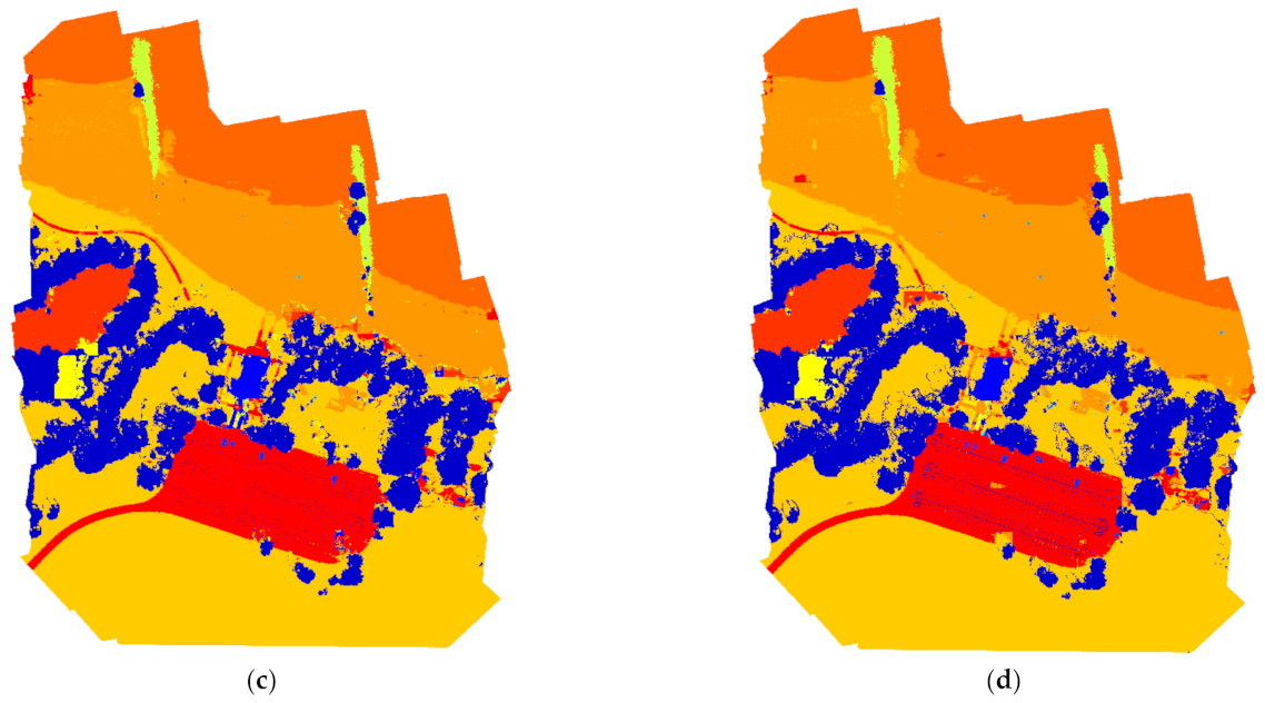
Figure 5.
RIT-18 segmentation results for Swin-tiny on the test image: (a) ground truth, (b) segmentation map using the DF approach, (c) segmentation map using the SGS approach, (d) segmentation map using LC-Net.
Figure 5.
RIT-18 segmentation results for Swin-tiny on the test image: (a) ground truth, (b) segmentation map using the DF approach, (c) segmentation map using the SGS approach, (d) segmentation map using LC-Net.


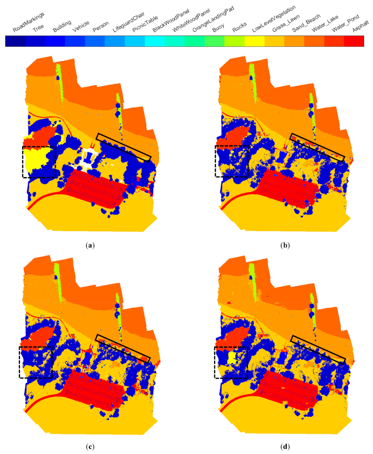
Figure 6.
RIT-18 segmentation results of the test image: (a) ground truth, (b) segmentation map from ResNet50+ LC-Net, (c) segmentation map from HRNet-w18+ LC-Net, (d) segmentation map from Swin-tiny+ LC-Net.
Figure 6.
RIT-18 segmentation results of the test image: (a) ground truth, (b) segmentation map from ResNet50+ LC-Net, (c) segmentation map from HRNet-w18+ LC-Net, (d) segmentation map from Swin-tiny+ LC-Net.

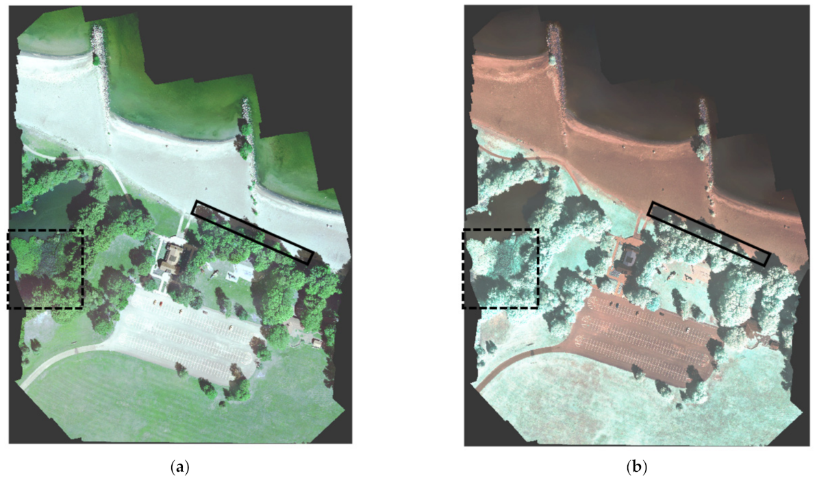
Figure 7.
(a) RGB image (bands 3, 2, and 1) of the RIT-18 test image; (b) pseudo color image of bands 4–6 of the RIT-18 test image.
Figure 7.
(a) RGB image (bands 3, 2, and 1) of the RIT-18 test image; (b) pseudo color image of bands 4–6 of the RIT-18 test image.

Figure 8.
The effect of the addition of LC-Net on the segmentation accuracy of different classes against the DF approach (%).
Figure 8.
The effect of the addition of LC-Net on the segmentation accuracy of different classes against the DF approach (%).


Table 1.
Summary of five commonly used multispectral datasets.
| Dataset | Sensor(s) | GSD (m) | Number of Classes | Number of Bands | Distribution of Bands |
|---|---|---|---|---|---|
| Vaihingen | Green/Red/IR | 0.09 | 5 | 3 | Green, Red, IR |
| Potsdam | VNIR | 0.05 | 5 | 4 | Blue, Green, Red, NIR |
| Zurich Summer | QuickBird | 0.61 | 8 | 4 | Blue, Green, Red, NIR |
| L8 SPARCS | Landsat 8 | 30 | 5 | 10 | Coastal, Green, Red, NIR, SWIR-1, SWIR-2, Pan, Cirrus, TIRS |
| RIT-18 | VNIR | 0.047 | 18 | 6 | Blue, Green, Red, NIR-1, NIR-2, NIR-3 |
Table 2.
Detailed architecture specifications of ResNet50 and Swin-tiny, where the bracket indicates a residual block, and the number outside the brackets is the number of stacked blocks for the stage.
Table 2.
Detailed architecture specifications of ResNet50 and Swin-tiny, where the bracket indicates a residual block, and the number outside the brackets is the number of stacked blocks for the stage.
| Output Size | ResNet50 | Swin-Tiny | |||
|---|---|---|---|---|---|
| Stem | , 64, stride 2 max pool, stride 2 | , 96, stride 4 | |||
| Resolution 1 | |||||
| Resolution 2 | |||||
| Resolution 3 | |||||
| Resolution 4 | |||||
| FLOPs | |||||
| Parameters | |||||
Table 3.
Detailed architecture specifications of HRNet-w18, where the bracket indicate a residual block, and the number outside the brackets is the number of stacked blocks for the stage.
Table 3.
Detailed architecture specifications of HRNet-w18, where the bracket indicate a residual block, and the number outside the brackets is the number of stacked blocks for the stage.
| Output Size | Stem | Stage 1 | Stage 2 | Stage 3 | Stage 4 | |
|---|---|---|---|---|---|---|
| Resolution 1 | , 64, stride 2 , 64, stride 2 | |||||
| Resolution 2 | ||||||
| Resolution 3 | ||||||
| Resolution 4 | ||||||
| FLOPs | ||||||
| Parameters | ||||||
Table 4.
Summary of the key performance of PCA, DF, LC-NET, and CoinNet (%).
| Class | ResNet50 | HRNet-w18 | Swin-Tiny | CoinNet | ||||||
|---|---|---|---|---|---|---|---|---|---|---|
| PCA | DF | LC-Net | PCA | DF | LC-Net | PCA | DF | LC-Net | - | |
| Road Markings | 0.0 | 33.6 | 40.6 | 0.0 | 3.2 | 73.3 | 0.0 | 13.3 | 63.1 | 85.1 |
| Tree | 72.7 | 91.5 | 90.1 | 8.8 | 78.1 | 85.4 | 80.2 | 82.1 | 88.3 | 77.6 |
| Building | 13.3 | 54.4 | 69.2 | 0.0 | 58.0 | 62.2 | 0.0 | 61.3 | 65.0 | 52.3 |
| Vehicle | 0.0 | 50.5 | 53.2 | 0.0 | 54.6 | 55.7 | 0.0 | 38.5 | 49.5 | 59.8 |
| Person | 0.0 | 0.0 | 0.0 | 0.0 | 0.0 | 0.0 | 0.0 | 0.0 | 0.0 | 0.0 |
| Lifeguard Chair | 0.0 | 82.1 | 66.3 | 0.0 | 32.2 | 79.5 | 0.0 | 39.1 | 99.5 | 0.0 |
| Picnic Table | 0.0 | 4.0 | 9.9 | 0.0 | 22.6 | 22.7 | 0.0 | 32.4 | 12.6 | 0.0 |
| Orange Pad | 0.0 | 0.0 | 0.0 | 0.0 | 95.8 | 0.0 | 0.0 | 83.1 | 0.0 | 0.0 |
| Buoy | 0.0 | 0.0 | 0.0 | 0.0 | 0.2 | 0.0 | 0.0 | 0.0 | 0.0 | 0.0 |
| Rocks | 1.2 | 84.3 | 93.3 | 5.3 | 73.1 | 91.5 | 4.0 | 88.0 | 90.3 | 84.8 |
| Low Vegetation | 0.0 | 1.7 | 4.9 | 0.6 | 11.4 | 5.6 | 0.0 | 2.9 | 19.0 | 4.1 |
| Grass/Lawn | 86.2 | 95.2 | 95.4 | 97.4 | 97.5 | 95.1 | 84.1 | 94.9 | 95.5 | 96.7 |
| Sand/Beach | 92.0 | 10.0 | 93.4 | 86.2 | 94.0 | 94.0 | 96.3 | 76.1 | 95.9 | 92.1 |
| Water/Lake | 58.2 | 96.9 | 97.6 | 89.3 | 95.9 | 98.1 | 93.4 | 98.8 | 94.3 | 98.4 |
| Water/Pond | 13.2 | 14.2 | 95.9 | 0.0 | 7.0 | 98.0 | 43.0 | 63.3 | 98.2 | 92.7 |
| Asphalt | 77.6 | 51.0 | 91.0 | 72.9 | 42.7 | 92.9 | 78.6 | 53.4 | 90.9 | 90.4 |
| Overall Accuracy | 73.8 | 68.7 | 90.7 | 69.5 | 82.4 | 90.4 | 81.2 | 84.6 | 91.0 | 88.8 |
| Mean Accuracy | 25.9 | 41.8 | 56.3 | 22.5 | 44.1 | 59.6 | 30.0 | 48.0 | 60.1 | 52.1 |
Table 5.
Comparison of accuracies and computational cost using PCA, DF, LC-Net, and SGS (%). The numbers shown in the “Input Method” column for SGS indicate which three bands were used as the input images to the subsequent networks.
Table 5.
Comparison of accuracies and computational cost using PCA, DF, LC-Net, and SGS (%). The numbers shown in the “Input Method” column for SGS indicate which three bands were used as the input images to the subsequent networks.
| Input Method | ResNet50 | HRNet-w18 | Swin-Tiny | |||||||
|---|---|---|---|---|---|---|---|---|---|---|
| OA | MA | Training Hours | OA | MA | Training Hours | OA | MA | Training Hours | ||
| PCA | 73.8 | 25.9 | 3.6 | 69.5 | 22.5 | 3.9 | 81.2 | 30 | 4 | |
| DF | 68.7 | 41.8 | 3.6 | 82.4 | 44.1 | 3.9 | 84.6 | 48 | 4 | |
| LC-Net | 90.7 | 56.3 | 3.6 | 90.4 | 59.6 | 3.9 | 91.0 | 60.1 | 4 | |
| SGS | 123 | 72.6 | 39.7 | 72 | 72.3 | 43.0 | 77 | 72.8 | 43.5 | 80 |
| 124 | 88.7 | 53.2 | 88.4 | 56.5 | 88.9 | 57.0 | ||||
| 125 | 86.7 | 51.4 | 86.4 | 54.7 | 87.0 | 55.2 | ||||
| 126 | 88.6 | 53.1 | 88.3 | 56.4 | 88.9 | 56.9 | ||||
| 134 | 85.4 | 53.2 | 85.1 | 56.5 | 85.7 | 57.0 | ||||
| 135 | 78.8 | 43.3 | 78.4 | 46.6 | 79.1 | 47.1 | ||||
| 136 | 74.5 | 43.8 | 74.1 | 47.1 | 74.7 | 47.6 | ||||
| 145 | 88.8 | 51.2 | 88.5 | 54.5 | 89.1 | 55.0 | ||||
| 146 | 86.4 | 52.8 | 86.1 | 56.1 | 86.6 | 56.6 | ||||
| 156 | 89.3 | 54.4 | 89.8 | 57.7 | 89.6 | 58.2 | ||||
| 234 | 86.3 | 51.9 | 85.9 | 55.2 | 86.5 | 55.7 | ||||
| 235 | 78.5 | 51.5 | 78.2 | 54.8 | 78.7 | 55.3 | ||||
| 236 | 81.0 | 44.1 | 80.7 | 47.3 | 81.3 | 47.8 | ||||
| 245 | 87.8 | 53.3 | 87.4 | 56.6 | 88.1 | 57.1 | ||||
| 246 | 85.4 | 49.6 | 85.1 | 52.9 | 85.7 | 53.4 | ||||
| 256 | 88.2 | 51.4 | 87.9 | 54.7 | 88.5 | 55.2 | ||||
| 345 | 89.3 | 50.7 | 88.9 | 54.0 | 89.5 | 54.5 | ||||
| 346 | 89.1 | 53.7 | 88.8 | 57.0 | 89.4 | 57.5 | ||||
| 356 | 89.4 | 55.7 | 89.0 | 57.8 | 89.8 | 59.3 | ||||
| 456 | 47.5 | 33.5 | 47.2 | 36.8 | 47.8 | 37.3 | ||||
Table 6.
Performance of LC-Net and LCAB (%).
| Methods | The Formation of 3 Input Bands to the Networks from the Original 6 Bands | ResNet50 | HRNet-w18 | Swin-Tiny | |||
|---|---|---|---|---|---|---|---|
| OA | MA | OA | MA | OA | MA | ||
| LC-Net | (12), (34), (56) | 90.7 | 56.3 | 90.4 | 59.6 | 91.0 | 60.1 |
| LC-Net (non-adjacent) | (13), (25), (46) | 90.8 | 56.2 | 90.2 | 59.4 | 91.2 | 59.0 |
| LCAB | (1–6), (1–6), (1–6) | 84.1 | 53.4 | 87.1 | 54.2 | 88.6 | 55.0 |
Table 7.
Final weights in LC-Net used in the three networks considered.
| Final Weights in LC-Net | |||
|---|---|---|---|
| ResNet50 + LC-Net | HRNet-w18 + LC-Net | Swin-tiny + LC-Net | |
| Band 1 | 0.048 | −0.066 | 0.253 |
| Band 2 | −0.893 | 0.201 | −0.159 |
| Band 3 | 0.927 | −0.464 | 0.220 |
| Band 4 | 1.100 | −0.722 | 0.470 |
| Band 5 | −0.931 | −0.555 | 0.530 |
| Band 6 | 0.460 | −0.417 | 0.348 |
Publisher’s Note: MDPI stays neutral with regard to jurisdictional claims in published maps and institutional affiliations. |
© 2022 by the authors. Licensee MDPI, Basel, Switzerland. This article is an open access article distributed under the terms and conditions of the Creative Commons Attribution (CC BY) license (https://creativecommons.org/licenses/by/4.0/).
Share and Cite
MDPI and ACS Style
Cai, Y.; Fan, L.; Zhang, C. Semantic Segmentation of Multispectral Images via Linear Compression of Bands: An Experiment Using RIT-18. Remote Sens. 2022, 14, 2673. https://doi.org/10.3390/rs14112673
AMA Style
Cai Y, Fan L, Zhang C. Semantic Segmentation of Multispectral Images via Linear Compression of Bands: An Experiment Using RIT-18. Remote Sensing. 2022; 14(11):2673. https://doi.org/10.3390/rs14112673
Chicago/Turabian StyleCai, Yuanzhi, Lei Fan, and Cheng Zhang. 2022. "Semantic Segmentation of Multispectral Images via Linear Compression of Bands: An Experiment Using RIT-18" Remote Sensing 14, no. 11: 2673. https://doi.org/10.3390/rs14112673
Note that from the first issue of 2016, this journal uses article numbers instead of page numbers. See further details here.