Integrating the Textural and Spectral Information of UAV Hyperspectral Images for the Improved Estimation of Rice Aboveground Biomass

Abstract

The accurate and rapid estimation of the aboveground biomass (AGB) of rice is crucial to food security. Unmanned aerial vehicles (UAVs) mounted with hyperspectral sensors can obtain images of high spectral and spatial resolution in a quick and effective manner. Integrating UAV-based spatial and spectral information has substantial potential for improving crop AGB estimation. Hyperspectral remote-sensing data with more continuous reflectance information on ground objects provide more possibilities for band selection. The use of band selection for the spectral vegetation index (VI) has been discussed in many studies, but few studies have paid attention to the band selection of texture features in rice AGB estimation. In this study, UAV-based hyperspectral images of four rice varieties in five nitrogen treatments (N0, N1, N2, N3, and N4) were obtained. First, multiple spectral bands were used to identify the optimal bands of the spectral vegetation indices, as well as the texture features; next, the vegetation index model (VI model), the vegetation index combined with the corresponding-band textures model (VI+CBT model), and the vegetation index combined with the full-band textures model (VI+FBT model) were established to compare their respective rice AGB estimation abilities. The results showed that the optimal bands of the spectral and textural information for AGB monitoring were inconsistent. The red-edge and near-infrared bands demonstrated a strong correlation with the rice AGB in the spectral dimension, while the green and red bands exhibited a high correlation with the rice AGB in the spatial dimension. The ranking of the monitoring accuracies of the three models, from highest to lowest, was: the VI+FBT model, then the VI+CBT model, and then the VI model. Compared with the VI model, the R² of the VI+FBT model and the VI+CBT model increased by 1.319% and 9.763%, respectively. The RMSE decreased by 2.070% and 16.718%, respectively, while the rRMSE decreased by 2.166% and 16.606%, respectively. The results indicated that the integration of vegetation indices and textures can significantly improve the accuracy of rice AGB estimation. The full-band textures contained richer information that was highly related to rice AGB. The VI model at the tillering stage presented the greatest sensitivity to the integration of textures, and the models in the N3 treatment (1.5 times the normal nitrogen level) gave the best AGB estimation compared with the other nitrogen treatments. This research proposes a reliable modeling framework for monitoring rice AGB and provides scientific support for rice-field management.

1. Introduction

Rice (Oryza sativa L.) is one of the most important grains in the world [1]. Aboveground biomass (AGB) plays a fundamental role in crop management and yield estimation [2]. Real-time AGB estimations provide the basis for field nitrogen control [3]. The timely and nondestructive monitoring of rice AGB is a prerequisite for ensuring rice production [4]. Conventional rice AGB estimation approaches, such as field campaigns, are not only time-consuming, costly, and destructive, but also ineffective for achieving large-scale monitoring in farmyard management [5]. By contrast, applications of remote sensing techniques have indicated great potential for estimating AGB due to their large-scale coverage, periodic dynamic monitoring, and non-destructiveness [6,7].

Using the vegetation indices (VIs) extracted from remote-sensing images to monitor biomass is the most commonly applied method [8,9]. VIs are usually constructed by mathematical operations on remotely sensed bands to take full advantage of spectral information and enhance vegetation characteristics [10]. Considerable attention has been paid to the application of VIs in estimating AGB due to their simplicity and easy use [11]. Nonetheless, it was proven that the vegetation index was easily disturbed by environmental factors, such as noise and soil [9]. Relying on VIs alone may not generate promising results. In addition to spectral information, remotely sensed images can also offer spatial information [12]. The texture feature is a vital presentation of spatial information, which represents the neighborhood characteristics of image pixels [13]. Integrating vegetation indices with textures can further reduce noise and background disturbance, helping to overcome the saturation problem at high biomass levels and improve model performance.

Some studies have already calculated vegetation indices and textures from satellite remote sensing data to estimate the forest leaf area index [14], forest biomass [15], grassland carbon [16], etc. However, the texture analyses of these studies were mostly based on large-scale ecosystems, such as forests and grasslands. Few studies have used the texture features of satellite remote-sensing images to monitor farmland ecosystems. This is mainly because satellite remote-sensing platforms featuring coarse resolution, long access periods, and weather influence cannot measure the spatial changes in field crops accurately [17]. Although satellite remote sensing with high spatial resolution offers sub-meter data, it does not easily provide detailed crop phenotypic information or meet the requirements of field-scale crop-growth monitoring [18]. In recent years, the emerging unmanned aerial vehicle (UAV) technology, which features low costs, high spatial and spectral resolution, and easy availability, has compensated for the disadvantages of satellite platforms [19]. UAV hyperspectral platforms that are capable of obtaining crop canopy images with abundant spatial and spectral information are gradually being applied in farmland ecosystems [12]. The textures of crops can reflect the dynamic changes in crop organs, plants, and backgrounds, which represent the spatial information of crop growth [20].

UAV remote sensing can be divided into two groups: hyperspectral remote sensing and multispectral remote sensing [21]. Multispectral images can be operated easily [22], but multispectral sensors only capture discrete spectral regions centered on specific wavelengths, making the bandwidths large (10–40 nm on average) [23]. The limited bands of multispectral images impede the band selection of the vegetation index to a certain extent [24]. Additionally, multispectral images contain less spectral information compared with hyperspectral images [25]. Board bands do not easily respond to the narrow spectral features of ground objects, hindering the band selection and influencing the accuracy and stability improvement of crop-growth models [26]. In contrast to multispectral data, hyperspectral images offer more continuous spectral and spatial information on objects through visible-to-near-infrared wavelengths [22]. Hyperspectral images have more and narrower bands (their bandwidth is typically less than 10 nm); therefore, they can offer more possibilities to the band selection of vegetation indices and texture features. Using hyperspectral information to build the vegetation index can further reduce noise and soil interference and describe vegetation canopy reflectance in greater detail [23,27]. The integration of spectral-spatial information from UAV hyperspectral data has been successfully applied in crop disease monitoring [28], yield estimation [29], nitrogen monitoring [30], etc., and demonstrated reliable outcomes. Previous studies proved that UAV hyperspectral images with high spectral and spatial resolution had great potential for crop-growth monitoring [4]. Relatively few studies have investigated the feasibility of integrating spectral and spatial information from UAV hyperspectral images to monitor rice AGB.

Selecting appropriate spectral and textural bands from hyperspectral images plays a central role in AGB estimation [31]. Previous studies mostly explored the influence of band selection on the vegetation index, such as narrowband and broadband [24,32]. However, the effect of the band selection of texture features on model performance was not considered. At different stages of growth, the nutrition absorption and environmental impact factors are diverse. The sizes and shapes of rice plants are different, even at the same growth stage. Studies showed that the establishment of multi-temporal models that included the characteristics of multiple growth stages were crucial for rice-growth management [33]. Studies focused on using multi-growth models to estimate rice yield [33], leaf area index [34], nitrogen [20], etc. have been carried out, but no attempt has been made to examine rice AGB estimates.

In this study, hyperspectral information was used to build vegetation indices and the spatial information of the textures extracted by the gray-level co-occurrence matrix (GLCM) was tested for improving VI-based models. Three kinds of the tillering–jointing–booting model, including the vegetation index combined with the full-band textures model (VI+FBT model), the vegetation index combined with the corresponding-band textures model (VI+CBT model), and the vegetation index model (VI model) were constructed by linear regression and multiple linear regression. The main objectives of this study were: (1) to determine the sensitive bands of the vegetation indices in the spectral dimension and the sensitive bands of the texture features in the spatial dimension, and identify the optimal form of integration of spectral-spatial information to improve rice AGB estimation; (2) to explore whether the integration of spectral-spatial information can increase the accuracy of rice AGB estimations, and analyze the improvements in the VI+FBT model and the VI+CBT model compared with the VI model; and (3) to compare the models’ performances according to various nitrogen levels and growth stages.

2. Materials and Methods

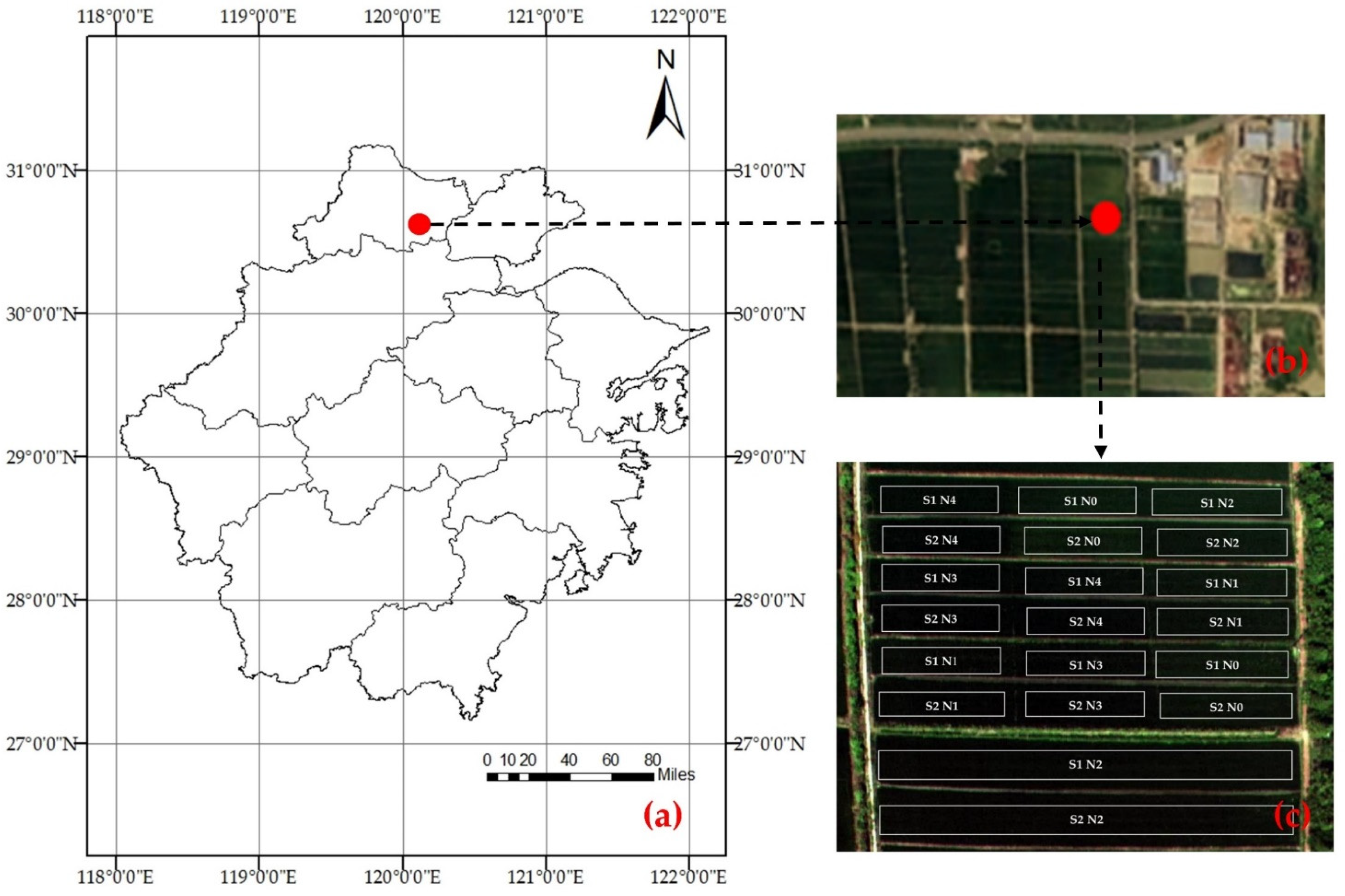
2.1. Study Area

The field experiment was conducted in Xiashe Village, Deqing County, Zhejiang province, China (120°10′51.20″E, 30°34′21.00″N) (Figure 1a). The study site is located in the western part of Hangjiahu Plain, which has a long history of rice production. Xiashe Village is a demonstration area for precision agriculture in Deqing County, which is characterized by a typical subtropical monsoon climate. The warm and humid climate favors the cultivation of rice.

2.2. Field Experiments

The experimental field was about 81 m wide in the east–west direction and 101 m long in the north–south direction, with a total area of 0.82 hectares and an average elevation of 5 m (Figure 1b,c). The total field was divided into twenty plots, of which eighteen had a total area of 81 m × 7 m, while the remaining two plots had a total area of 81 m × 21 m. Two rice varieties were adopted during each experimental year, in accordance with the most widely planted rice cultivars in local farmland. The selected varieties were: Zhejing 99 (S1) and Jia 67 (S2) in 2018, and Nanjing 9108 (S1) and Nanjing 46 (S2) in 2019. Considering the interaction of the general environment with water, nitrogen treatments were prevented from seeping into other plots. Five nitrogen rates were set to grant varied rice AGB, including N0 (0 kg ha⁻¹), N1 (112.5 to 142.5 kg ha⁻¹, 0.5 times the nitrogen application level of the local farmers), N2 (225 to 285 kg ha⁻¹, the normal level used by the local farmers), N3 (337.5 to 427.5 kg ha⁻¹, 1.5 times the normal level), and N4 (450 to 570 kg ha⁻¹, twice the normal level) [35]. The phosphate and potash fertilizers were 75 kg ha⁻¹ and 150 kg ha⁻¹, respectively. All treatments contained two or more repeated plots.

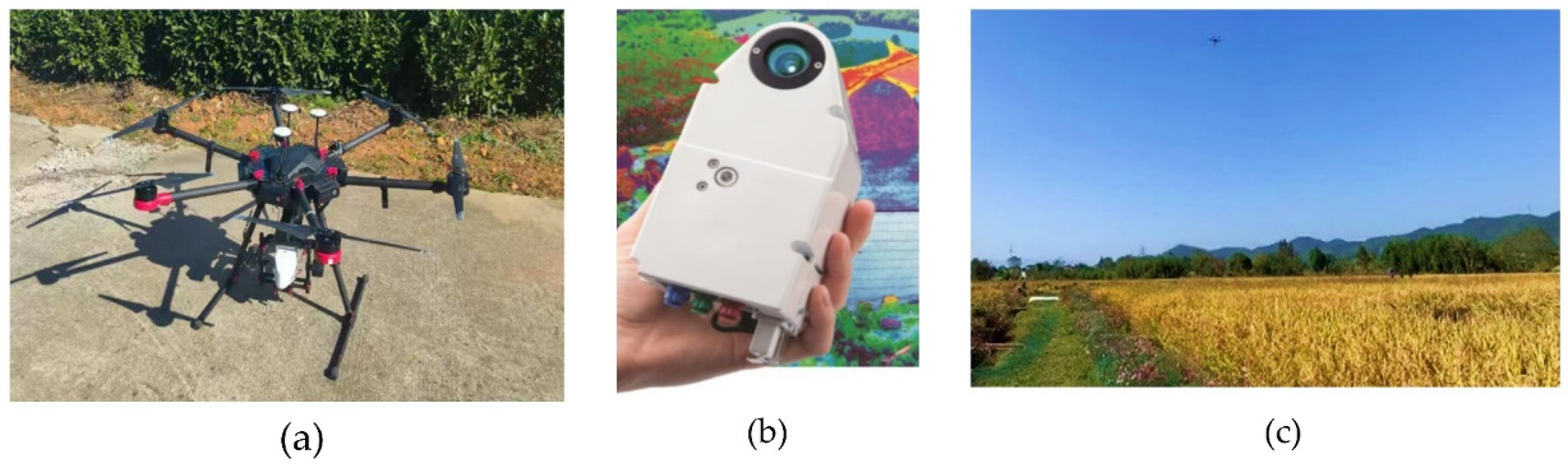
2.3. UAV-Based Hyperspectral Image Acquisition and Preprocessing

A six-rotor UAV (DJI M600 Pro) equipped with a Rikola hyperspectral camera (Figure 2b) was used to acquire remote-sensing images of rice (Figure 2a). The number of bands was 62, ranging from 500–900 nm. The acquisitions of UAV images were conducted between 10:00 a.m. and 14:00 p.m. on sunny and cloudless days (Figure 2c). Each flight had a fixed route and a fixed altitude of 200 m, with a ground spatial resolution of 13 cm. The exposure time of the hyperspectral camera was adjusted according to the lighting conditions.

Rikola hyperspectral camera can finish imaging of the same band at once and the data of all pixels are real radiance values without interpolation [36]. The images taken by the Rikola camera during the flight were stored on the memory card. The hyperspectral images were preprocessed to obtain field canopy reflectance. The raw data were preprocessed through dark-current correction, halo correction, and distortion correction to convert DN values into radiation values in Rikola hyperspectral imager V2.1.4 (Rikola Ltd., Oulu, Finland) and band registration by RegMosaic (Rikola, Ltd.). Radiometric correction was performed using the reference board with fixed reflectance on the ground. The equation of radiometric correction (Equation (1)) was used to calculate the reflectance of images:

$${\mathrm{Ref}}_{\mathrm{img}}=\frac{{\mathrm{Rad}}_{\mathrm{img}}\times {\mathrm{Ref}}_{\mathrm{grey}}}{{\mathrm{Rad}}_{\mathrm{grey}}}$$

(1)

Rad_img represents the radiation of the image. Rad_grey represents the radiation of the reference board, and Ref_grey represents the reflectance of the reference board. Rad_grey could be obtained by setting a diffuse reflectance area in the UAV images. Ref_grey could be obtained by choosing a standard curve corresponding to the spectralon cloth.

2.4. AGB Measurement

At the tillering stage, jointing stage, and booting stage, rice plants in an area of 2 × 2 plots with uniform growth were sampled from south to north for AGB measurement (Figure 3). The rice roots were cut off and the aboveground parts of the leaves and stems were separated; then, they were weighed to obtain the fresh weight of leaves and stems. After weighing, all samples were put into paper bags and placed in an oven at 105 °C for 40 min, and oven-dried at 65 °C until reaching constant weight. The AGB per unit area was calculated as follows:

$$\mathrm{AGB}=\frac{\mathrm{Dry} \mathrm{leaf} \mathrm{weight}+\mathrm{Stem} \mathrm{weight}}{\mathrm{Number} \mathrm{of} \mathrm{sampled} \mathrm{plants}}\times \mathrm{Stems} \mathrm{per} \mathrm{hectare}$$

(2)

2.5. Calculations of Vegetation Index and Texture Features

2.5.1. Calculations of Vegetation Index

Vegetation indices are different types of remote sensing variants composed of multiple spectral bands with different reflection characteristics through linear and nonlinear calculations. They can indicate changes in plant growth parameters such as chlorophyll content [37], leaf area index [38], biomass [4], etc. They have been used as reliable indicators of AGB to evaluate vegetation coverage and growth vitality [10]. The main advantages of hyperspectral remote sensing are the strong band continuity and abundant spectral bands, which can monitor crop group information in a more refined manner [4]. The normalized difference vegetation index (NDVI), ratio vegetation index (RVI), and difference vegetation index (DVI) are widely used in crop growth monitoring, and were proven to be highly correlated to AGB. These three indices also represent the combination characteristics of most vegetation indices. Pairwise combinations of 62 bands from UAV hyperspectral images were used to construct all possible NDVI, DVI, and RVI results in this study (

Table 1. The calculation formulae for vegetation indices.

Vegetation Indices	Formulas	Reference
Normalized difference vegetation index, NDVI	$\mathrm{NDVI}=\left({\rho }_{\lambda }-{\rho }_{\mu }\right)$$/({\rho }_{\lambda }+{\rho }_{\mu }$)	[39]
Ratio vegetation index, RVI	$\mathrm{RVI}={\rho }_{\lambda }$$/{\rho }_{\mu }$	[40]
Difference vegetation index, DVI	$\mathrm{DVI}={\rho }_{\lambda }-{\rho }_{\mu }$	[41]

Note: λ and μ are the wavelengths of 62 bands in the range of 500–900 nm.

).

2.5.2. Calculations of Spatial Features

There are many methods for describing image spatial features, including statistical methods, model methods, geometric methods, structural analysis methods, etc. [42]. The grey-level co-occurrence matrix (GLCM) is one of the most widely used texture extraction methods: it was proposed by Haralick in 1973 [43]. Many scholars use GLCMs, due to their ability to ensure the non-deformation, multiscale features of rotation and the low complexity of calculations [44]. In this study, eight commonly used texture features were extracted from the UAV hyperspectral images (

Table 2. Calculation formula of texture features.

Texture	Formula	Meaning
Mean (MEA)	${\displaystyle {\displaystyle \sum }_i}{\displaystyle {\displaystyle \sum }_j}x\left(i,j\right)p\left(i,j\right)$	The overall grey level in the GLCM window.
Variance (VAR)	${\displaystyle {\displaystyle \sum }_i}{\displaystyle {\displaystyle \sum }_j}{\left(i-u\right)}^{2}p\left(i,j\right)$	The change in grey level variance in the GLCM window.
Homonity (HOM)	${\displaystyle {\displaystyle \sum }_i}{\displaystyle {\displaystyle \sum }_j}\frac{1}{1+{(i-j)}^2}p\left(i,j\right)$	The homogeneity of grey level in the GLCM window.
Contrast (CON)	${\displaystyle {\displaystyle \sum }_{n=0}^{N_g-1}}{n}^2{\left\{{\displaystyle {\displaystyle \sum }_{i=1}^{N_g}}{\displaystyle {\displaystyle \sum }_{j=1}^{N_g}}p\left(i,j\right)\right\}}_{\left|i-j\right|=n}$	The clarity of texture in the GLCM window, as opposed to HOM.
Dissimilarity (DIS)	${\displaystyle {\displaystyle \sum }_{n=1}^{N_g-1}}n{\left\{{\displaystyle {\displaystyle \sum }_{i=1}^{N_g}}{\displaystyle {\displaystyle \sum }_{j=1}^{N_g}}p{\left(i,j\right)}^2\right\}}_{\left|i-j\right|=n}$	The similarity of the pixels in the GLCM window, similar to CON.
Entropy (ENT)	$-{{\displaystyle \sum }}_i{{\displaystyle \sum }}_{j}p\left(i,j\right)log\left(p\left(i,j\right)\right)$	The diversity of the pixels in the GLCM window, proportional to the complexity of the image texture.
Secondary moment (SEM)	${\displaystyle {\displaystyle \sum }_i}{\displaystyle {\displaystyle \sum }_j}p{\left(i,j\right)}^2$	The uniformity of greyscale in the GLCM window.
Correlation (COR)	$\frac{{{\displaystyle \sum }}_i{{\displaystyle \sum }}_{j}p\left(i,j\right)\left(ij\right)-{\mu }_x{\mu }_y}{{\sigma }_x{\sigma }_y}$	The ductility of the grey value in the GLCM window.

Note: i and j represent the row and column number, respectively. $x\left(i,j\right)$ represents the value of the matrix at the corresponding row and column. $p\left(i,j\right)$ represents the ratio of the value of the matrix at the corresponding row and column to the sum of all values in the matrix. $N_g$ represents the length (width) of the matrix. ${\mu }_x$ and ${\mu }_y$ represent the mean of the matrix in the x and y directions, respectively. ${\sigma }_x$ and ${\sigma }_y$ represent the variance of the matrix in the x and y directions, respectively [44].

). Choosing appropriate window sizes helped reflect the changes in spatial information between rice plants in the experimental plot. Windows which were too small increased the amount of calculation and computational complexity, whereas windows which were too large led to a loss of detailed texture information [45]. Taking the average value could synthesize the functions of different window sizes. Through a trial and error approach, the texture features were calculated using the average values of two window sizes (3 pixels × 3 pixels and 5 pixels × 5 pixels) with four directions (0°, 45°, 90°, and 135°) rotating clockwise along the x-coordinate axis.

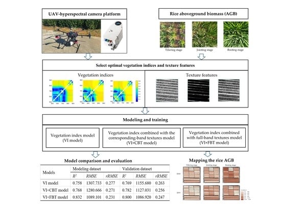
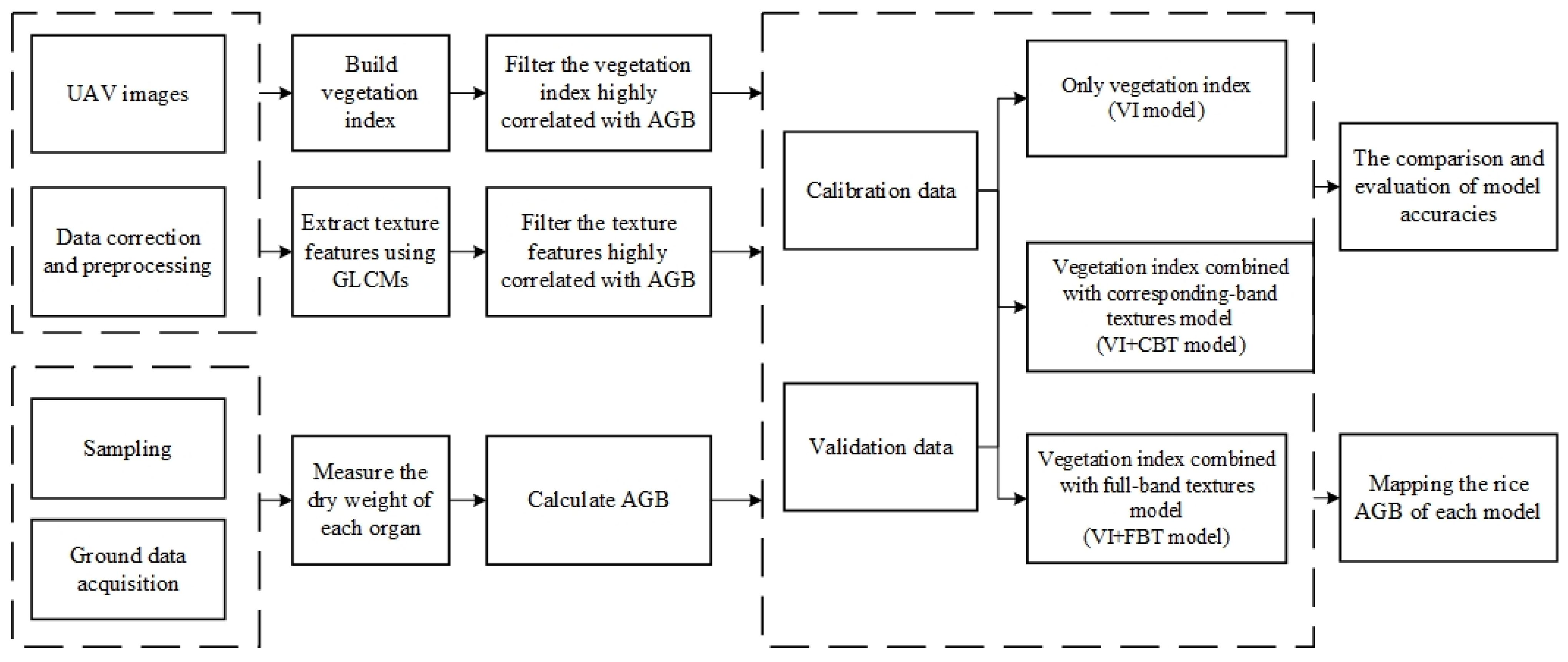
2.6. Model Construction and Evaluation

Previous research has shown that integrating spectral–spatial information could alleviate the saturation phenomenon as compared with using spectral information alone [12]. Three phenology stages before the flowering stage were considered: the tillering stage, the jointing stage, and the booting stage. The workflow for model construction included the following steps (Figure 4): (1) Correlation analysis was used to select the top ten vegetation indices highly correlated to AGB in each kind. Stepwise multiple regression was subsequently applied to extract the optimal textures and VIs; (2) Quantitative relationships between the optimal vegetation indices, texture features, and AGB were analyzed, and the multiple regression method was used to establish the VI, VI+CBT, and VI+FBT models; and (3) Accuracy assessments were conducted to evaluate the effect of each model.

2.6.1. Model Construction

This research focused on the improvement effects of integrating texture features and vegetation indices in AGB monitoring, rather than the comparison of different complicated artificial intelligence methods. Consequently, simple empirical methods were used to construct the models. Interpretable empirical models can explain the role of each variable in rice AGB models.

Redundancy and multicollinearity are two key aspects of hyperspectral data procession [46]. Multiple stepwise regression is an empirical method of variable selection with easy operability. The processes are: (1) calculate the sum of squares of partial regression for the variables that have been introduced into the regression equation, and then select a variable with the smallest sum of squares of partial regression; (2) a significance test at a predetermined level is performed. If a variable is significant, it is not necessary to exclude it from the regression equation. If a variable is not significant, it needs to be removed and other variables in the equation will be put through significance tests in order of the sum of squares of partial regression from small to large. The method can ascertain the most notable independent variables from many independent variables and remove the least influential variables through the test. Utilizing this method can eliminate multi-collinearity between the independent variables to achieve a more rational estimation effect [35,47]. Multiple linear regression is one of the most commonly used methods in empirical models. It calculates the best-fit equation by minimizing the sum of squares of vertical deviations from each data point to the diagonal to combine multiple explanatory variables [48]. The multiple stepwise regression method was employed to optimize vegetation indices and texture features which were highly correlated with AGB; then, multiple linear regression method was used to combine these optimal variables. The model expression was as follows:

$$y=k_0+k_1{x}_1+k_2{x}_2+k_3{x}_3\dots \dots k_n{x}_n$$

(3)

where y is the model-dependent variable, x₁ … x_n are all model-independent variables, and k₀ … k_n are all model coefficients.

2.6.2. Model Evaluation

All 120 AGB data values and corresponding spectral and spatial variables were randomly divided into three equal groups, with two-thirds of the dataset (n = 80) as the calibration dataset and one-third of the dataset (n = 40) as the validation dataset. To ensure that the two datasets were completely independent and the AGB estimation models were reliable, the greatest value of the validation dataset needed to fall in the range of the calibration dataset. The accuracy of the AGB model was evaluated using three indicators: the coefficient of determination (R²), the root-mean-square error (RMSE), and the relative root-mean-square error (rRMSE). R² reflects how well the AGB equation fits. RMSE shows the numerical difference between the estimated AGB and the actual AGB. The penalty coefficient is increased in the form of a square term when there is a large gap between the predicted and the true values. The prediction sensitivity of RMSE to outliers is relatively high. Therefore, the parameter is sensitive to over- and under-estimations of AGB. Moreover, rRMSE was used to prevent the RMSE from being affected by the dimension of the variables and compare different regression models with varied data amounts. The model with smaller rRMSE and RMSE values and a higher R² would have higher monitoring accuracy [4]. The formulae of these indicators are defined as:

$${\mathrm{R}}^2=1-\frac{{{\displaystyle \sum }}_i{\left(y-y^{\prime }\right)}^2}{{{\displaystyle \sum }}_i{\left(y-\overline{y}\right)}^2}$$

(4)

$$\mathrm{RMSE}=\sqrt{\frac{{{\displaystyle \sum }}_{i=1}^n{\left(y-y^{\prime }\right)}^2}{n}}$$

(5)

$$\mathrm{rRMSE}=\frac{\mathrm{RMSE}}{\overline{y}}$$

(6)

where y is the actual AGB data, y′ is the estimated AGB data, $\overline{y}$ is the average value of the AGB data, and n is the sample size.

3. Results and Analysis

3.1. AGB Data Statistical Analysis

The average AGB of the three growth stages of the samples was 4960.117 kg ha⁻¹ and the overall coefficient of variation was 0.607 (

Table 3. Statistical analysis of AGB values at different growth stages.

Growth Stage	AVG *	MIN.	MAX.	SD.	VAR.	CV(%)
Tillering stage	1869.305	498.667	6069.429	972.093	944,965.520	52.0
Jointing stage	5101.651	1900.444	9112.444	1884.780	3,552,394.162	36.9
Booting stage	7909.396	3424.667	12,707.840	2093.530	4,382,866.921	26.5
Tillering–jointing–booting stages	4960.117	498.667	12,707.840	3008.570	9,051,493.766	60.7

* AVG, MIN, MAX, SD, VAR, and CV(%) represent the average value, the minimum value, the maximum value, the standard deviation, the variance, and the coefficient of variation of the AGB, respectively.

). The minimum was 498.667 kg ha⁻¹, at the tillering stage, while the maximum was 12,707.840 kg ha⁻¹, at the booting stage. The most rapid accumulation of rice AGB occurred from the tillering stage to the booting stage. The average AGB at the tilling stage was 1869.305 kg ha⁻¹, while the average AGB at the booting stage increased to 7909.396 kg ha⁻¹. The tillering stage generated larger coefficient of variation values compared with the other stages.

3.2. Vegetation Index Selection and Vegetation-Index-Based AGB Model Construction

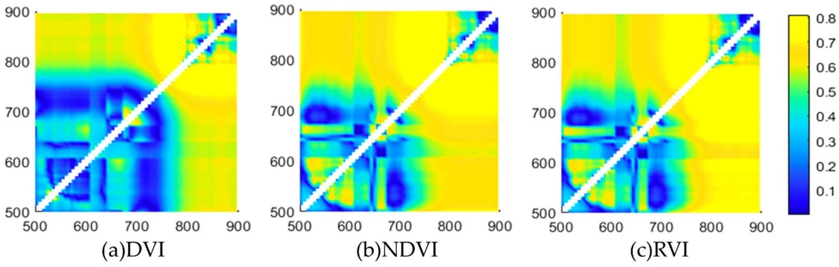
3.2.1. Vegetation Index Selection

The R² between the vegetation indices and the AGB were plotted onto two-dimensional distribution maps (Figure 5). The abscissa and ordinate of each pixel in the image corresponded to the construction bands of the vegetation index. The pixel value was the R² between the vegetation index and the rice AGB. The sensitive bands of the DVI, NDVI, RVI in the rice AGB estimation were concentrated in three spectral regions, respectively: (1) band 1, located at 700–800 nm, and band 2, located at 800–900 nm; (2) band 1,2 located around 680–700 nm; and (3) band 1, at 850–900 nm and band 2 at 800–820 nm. Additionally, these indices denoted some different spectral regions highly correlated with the rice AGB, respectively: band 1, at 500–600 nm, and band 2, at 650–660 nm, with both two bands were located around 520–600 nm (NDVI, RVI); band 1, at 750–900 nm, and band 2, at 500–700 nm (RVI); band 1, at 590–600 nm, and band 2, at 670–680 mn (DVI).

Pairwise combinations of 62 bands built a large number of vegetation indices. To reduce the workload of the data processing, the ten vegetation indices that correlated the most strongly with the rice AGB were selected (R² ≥ 0.7) (

Table 4. Selected vegetation indices and their corresponding bands.

Index	Selected Band Combination
DVI	(520,536)	(600,685)	(650,588)	(752,800)	(776,840)	(752,888)	(688,704)	(679,712)	(808,748)	(848,744)
NDVI	(528,685)	(568,760)	(696,768)	(691,879)	(760,699)	(768,664)	(784,700)	(800,504)	(800,685)	(888,504)
RVI	(504,568)	(551,671)	(584,536)	(685,576)	(744,800)	(776,720)	(792,848)	(800,724)	(824,728)	(840,744)

). The indices in the DVI type were constructed through the combination of the near-infrared band and the red-edge band, except those of DVI_(776,840), which were constructed by two near-infrared bands. The combination bands in the NDVI type were always near-infrared and red bands (such as 664 nm, 685 nm, and 700 nm). The RVI indices consisted of near-infrared and red-edge bands. In summary, the wavelength ranges of these vegetation indices were mostly concentrated in the red and near-infrared wavelength ranges.

3.2.2. Vegetation Index AGB Model Construction

The principle of the model’s establishment was to achieve the highest monitoring accuracy with the smallest number of independent variables. Vegetation indices can extract useful AGB-related information from original images, decreasing the complexity of hyperspectral-data processing [49]. The thirty selected vegetation indices were used as independent variables, while the AGBs were used as dependent variables in multiple stepwise multiple regression. The selected optimal indices were used to construct a VI model of rice AGB (Equation (7)):

$$\begin{array}{c}\mathrm{AGB}=74367.154-108433.135\times {\mathrm{DVI}}_{\left(808,748\right)}-79694.926\times {\mathrm{RVI}}_{\left(744,800\right)}\end{array}$$

(7)

The model was constructed by a DVI type and an RVI type of vegetation index, both of which were composed of red-edge and near-infrared bands. The NDVI type of vegetation index was not involved in the model. The potential explanation for this was that the density of the AGB was large at the booting stage, leading to the saturation of the plant coverage, which reduced the sensitivity of the NDVI to the AGB [50]. DVI and RVI vegetation indices are comparatively insensitive to the saturation phenomenon at high AGB [51]. The RVI vegetation index has a high correlation with AGB, which is a sensitive indicator parameter of green plants and high vegetation coverage [52].

3.3. Texture-Feature Selection and Coupled AGB Model Construction

3.3.1. Texture Features Selection

The hyperspectral image had 62 bands, and each band had eight texture features, resulting in a total of 62 × 8 = 496 texture features in every image. This inevitably caused the problems of enormous calculation and redundant information [46]. To alleviate the heavy computing task and eliminate the useless information, multiple stepwise regression (MSR) was used to select the optimal texture features (confidence interval = 95%). With the vegetation index corresponding-band textures (CBT) as inputs, three texture features (SEM₇₄₈, MEA₈₀₀, and MEA₈₀₈) were identified; they consisted of red-edge and near-infrared wavelengths. As for the full-band textures (FBT), five texture features were identified: COR₅₀₄ and ENT₅₃₆ in the green spectral region, ENT₅₈₄ in the yellow spectral region, and COR₆₅₀, COR₆₃₂, and COR₆₃₅ in the red spectral region (

Table 5. Selection of the possible texture features.

Bands	Filtered Textures
Vegetation index corresponding bands	SEM748		MEA800		MEA808
Full bands	COR504	ENT536	COR650	COR632	ENT584	COR635

).

3.3.2. Construction of Coupled Model Integrating Vegetation Indices with Corresponding-Band Textures

Due to the abundant textures and bands of the UAV hyperspectral images, the data computation posed many difficulties [46]. It was essential to determine the optimal band combination before the modeling. The CBT obtained both spectral and spatial information simultaneously, which can reduce the pressure of data processing and reduce the demand for spectral information. Therefore, the corresponding bands of the optimal vegetation index were first selected. The vegetation indices and corresponding-band textures were used as independent variables, while the AGB was used as the dependent variable in the modeling process. The model was as follows:

$$\begin{array}{c}\mathrm{AGB}=76025.147-107650.575\times {\mathrm{DVI}}_{\left(808,748\right)}-79953.278\times {\mathrm{RVI}}_{\left(744,800\right)}-8226.269\times {\mathrm{SEM}}_{748}\\ +389.704\times {\mathrm{MEA}}_{800}-406.731\times {\mathrm{MEA}}_{808}\end{array}$$

(8)

DVI_(808,748) and RVI_(744,800) were the parameters of the original vegetation index model, while the texture features SEM₇₄₈, MEA₈₀₀, and MEA₈₀₈ were selected as the optimal texture features for the rice AGB monitoring. The addition of the texture features improved the validation R² of the AGB model from 0.758 to 0.768 and of the testing R² from 0.769 to 0.782. The validation RMSE of the VI+CBT model decreased from 1307.733 to 1280.666, while the rRMSE decreased from 0.277 to 0.271. The test results using the validation dataset had similar trends to those obtained with the calibration dataset (

Table 6. Comparisons of the accuracy of three AGB models.

Models	Calibration Dataset			Validation Dataset
	R2	RMSE	rRMSE	R2	RMSE	rRMSE
Vegetation index model (VI model)	0.758	1307.733	0.277	0.769	1155.680	0.263
Vegetation index combined with corresponding-band texture model (VI+CBT model)	0.768	1280.666	0.271	0.782	1127.031	0.256
Vegetation index combined with full-band textures model (VI+FBT model)	0.832	1089.101	0.231	0.800	1086.920	0.247

Note: The presented values were rounded to three decimals for the sake of simplicity.

). The results showed that although the added textural information of the VIs per se improved the accuracy, the improvement was not very obvious.

3.4. Construction of Coupled Model Integrating Vegetation Indices with Full-Band Textures

In order to achieve higher accuracy in the rice AGB estimation, full-band textures were used in the modeling process. The VI+FBT model was as follows:

$$\begin{array}{c}\mathrm{AGB}=38762.457-20041.283\times {\mathrm{DVI}}_{\left(808,748\right)}-45243.297\ast {\mathrm{RVI}}_{\left(744,800\right)}+4376.107\times {\mathrm{COR}}_{504}+\\ 2554.066\times {\mathrm{ENT}}_{536}-4311.195\times {\mathrm{COR}}_{632}+5419.598\times {\mathrm{COR}}_{650}\end{array}$$

(9)

Compared with the VI model, the calibration and validation R² of the VI+FBT model increased by 9.763% and 4.031%, respectively, the RMSE decreased by 16.718% and 5.950%, respectively, and the rRMSE decreased by 16.606% and 6.084%, respectively. Compared with the VI+CBT model, the calibration and validation R² of the VI+FBT model increased by 8.333% and 2.302%, respectively, the RMSE decreased by 14.958% and 3.559%, respectively, and the rRMSE decreased by 14.760% and 3.516%, respectively. Unlike the VI+CBT model, this model used two new texture features (COR, ENT). The four bands were 504 nm and 536 nm in the green band and 632 nm and 650 nm in the red band. Although there were no green or red bands in the construction of the vegetation indices, the addition of full-band textures in these spectral regions could further enhance the ability to monitor rice AGB.

The AGB at tillering, jointing and heading stages were estimated using Equation (9), and subsequently the spatial distributions of AGB were mapped at plot scale in 2018 and 2019 (Figure 6). Considerable differences in AGB can be observed in the different growth stages and plots. The comparison between Figure 6 and Figure 1c showed that there was a certain amount of correlation between the nitrogen application level and the AGB. The AGB accumulated with the increase in nitrogen in a certain range. The AGB map intuitively expressed the spatial distribution of the AGB under three models and provided a scientific basis for future fertilization management [53].

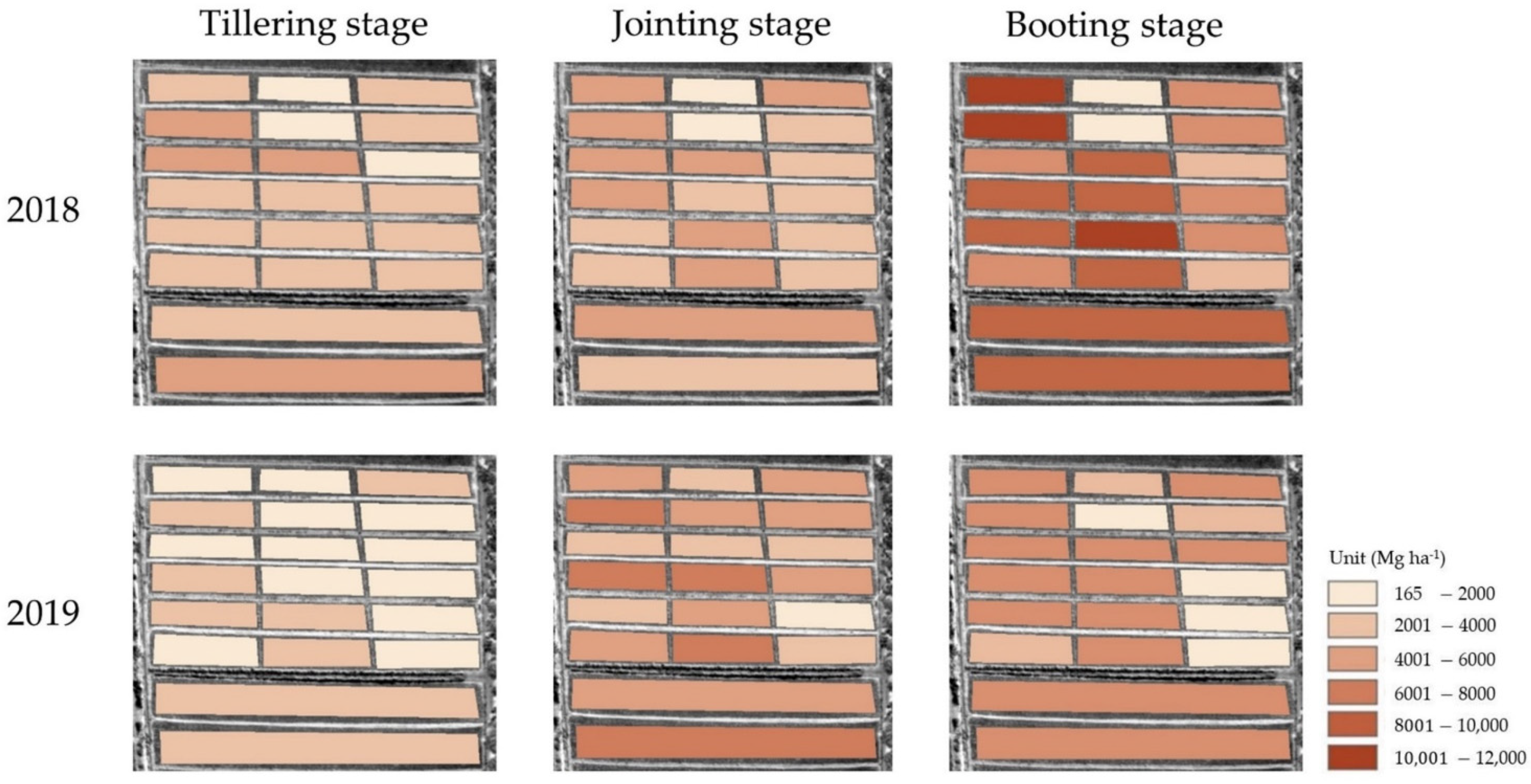
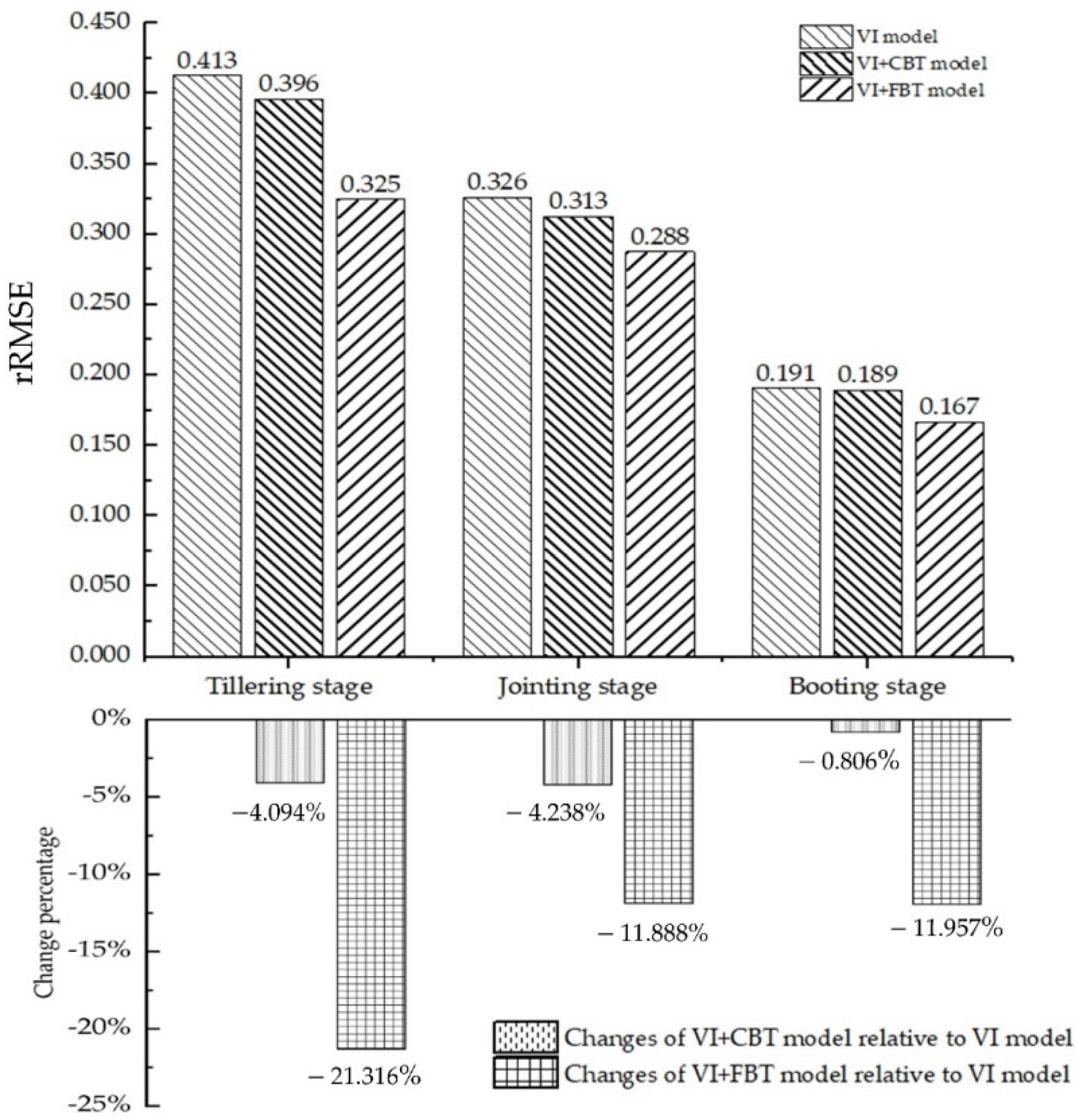
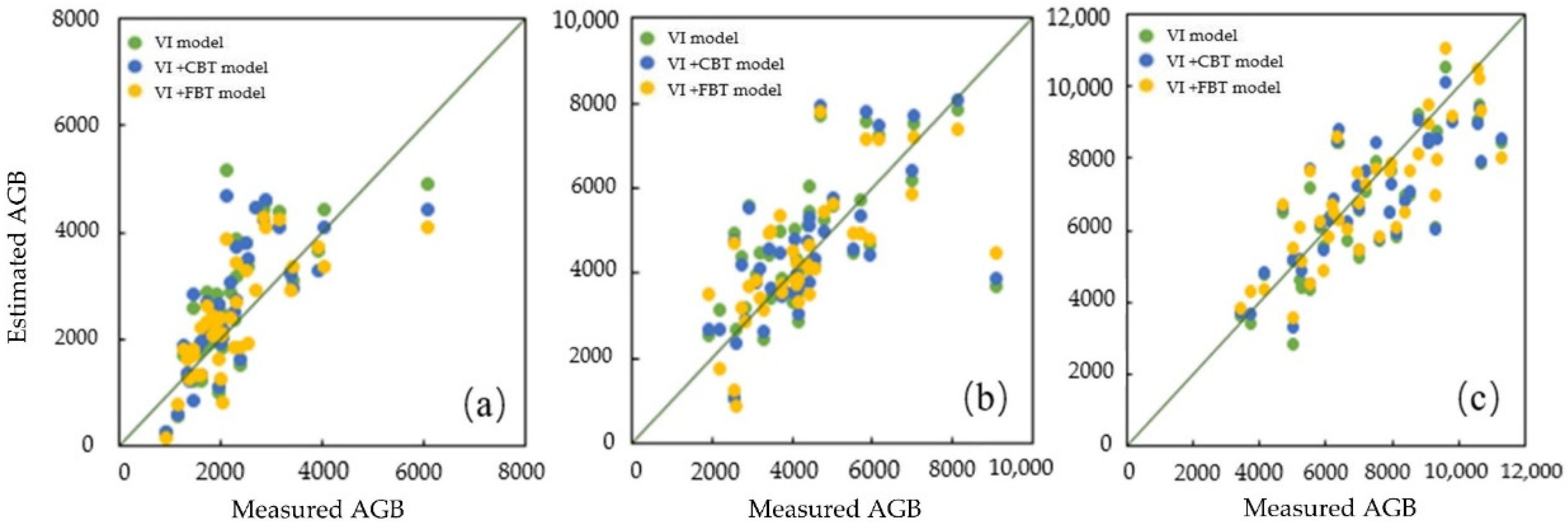
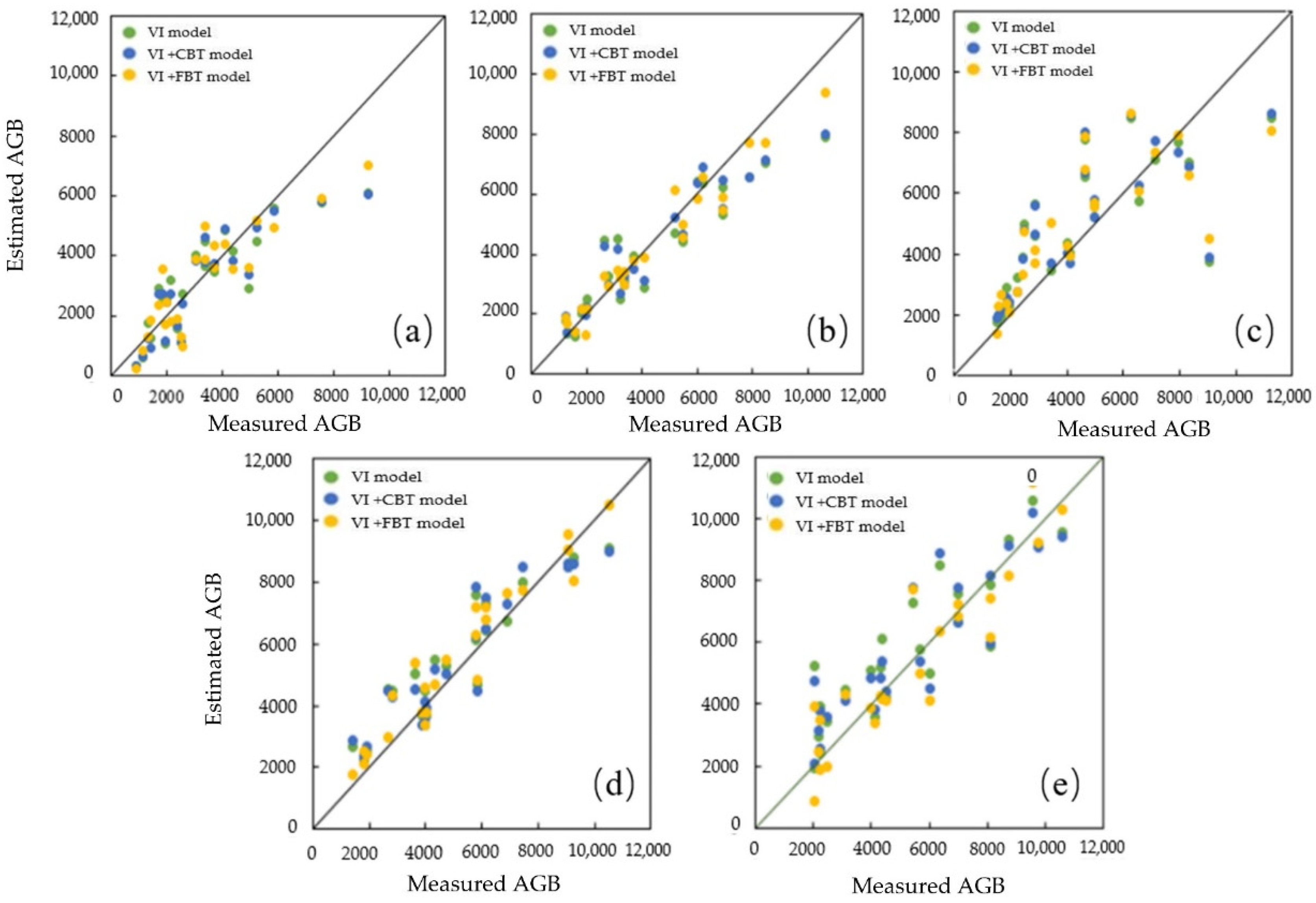
3.5. Effects of Growth Stages on Model Performance

The growth stage and nitrogen are two essential factors affecting rice AGB [54]. When developing three-period AGB estimation models utilizing VIs and texture features, it is necessary to fully consider the accuracy difference in each model, caused by the varied growth stage [55]. The AGB estimation model constructed in this research was a comprehensive model of three growth stages. The performances of each model at different growth stages were compared to explore the influences of the growth stages on the AGB estimations (Figure 7).

The rRMSE at the tillering stage was the largest, followed by the jointing stage and the booting stage, in the three models. These results indicated that the accuracy of the AGB estimation at the booting stage was highest, followed by the jointing stage and the tillering stage (Figure 7 and Figure 8). The VI model had the lowest AGB estimation accuracy and VI+CBT model improved the accuracy at each growth stage. The rRMSE was reduced by 4.094%, 4.238%, and 0.806% at the tillering stage, jointing stage, and booting stage, respectively. These results suggested that the corresponding-band textures had a good effect on the tillering and jointing stages, while their effect on the booting stage was not significant. When the band range was expanded to 500–900 nm, the rRMSE was reduced by 21.316%, 11.888%, and 11.957% at the tillering stage, jointing stage, and booting stage, respectively.

Figure 8 shows that the period from the tillering stage to the jointing stage was when the nitrogen absorption was the fastest, and the range of the AGB changed markedly. The nutrient accumulation of the rice essentially ended at this point, and the AGB reached its peak at the booting stage [56]. The addition of the texture features made the scattered AGB-value points more concentrated.

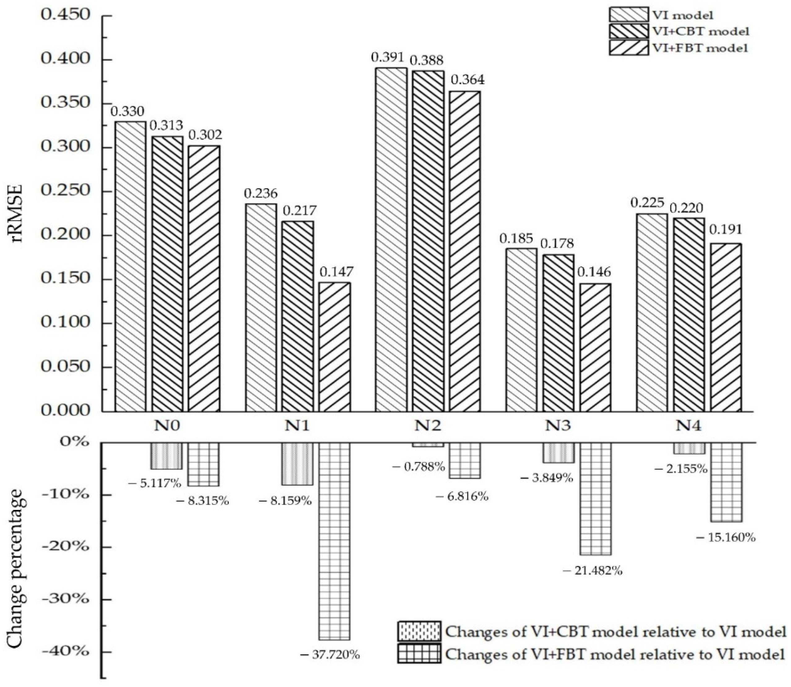
3.6. The Performance of Different Models under Various Nitrogen Gradients

Nitrogen management is a fundamental factor that must be regulated in field environments [57]. Fertilization can be guided by AGB monitoring [12,54]. This section provides an example of selecting the optimal model for monitoring rice AGB under different nitrogen levels, helping to reduce the input of manpower and material resources. The method improved the efficiency of the AGB monitoring and prevented the excessive application of nitrogen fertilizers from polluting the field environment.

The best estimation model was the VI+FBT model under N3 (rRMSE = 0.146), whose rRMSE was 21.482% lower than that of the VI model. The VI model under N1 responded the most sensitively to the integration of the textures, followed by N3 and N4 (Figure 9).

The overall AGB estimation error of the N3 and N1 was the smallest, and the AGB estimation effect of the N4 and N0 was slightly lower than that of the N3 and N1. The accuracy of the AGB estimation under the N0 was relatively low, and the AGB distribution of the N3 and N4 was the most consistent with the expected effect of the gradient design. Figure 10 shows that the AGB of the N4 had multiple overestimations and the AGB of the N1 had multiple underestimations. The data points were the most scattered, with multiple values deviating far from the 1:1 line, under the N2, indicating that the estimation accuracy was low. These results illustrated that higher nitrogen concentrations may not lead to greater AGB accumulation. If excessive nitrogen is applied to fields, it destroys crop growth. If crops lack nitrogen, their roots are unable to absorb enough nutrition, and the plants grow poorly [58].

4. Discussion

4.1. The Sensentive Bands of the Vegetation Indices and Texture Features for Rice AGB Estimation

The rich spectrum of UAV hyperspectral data laid a good foundation for the band selection of the vegetation index and texture features [32]. The vegetation indices in the DVI, NDVI, and RVI types for rice AGB estimation in this research were mainly composed of near-infrared (such as 800 nm, 808 nm, etc.) and red-edge (such as 748 nm, 744 nm, etc.) bands, which were slightly different from the conventional VIs constructed by the near-infrared and red bands. Some studies showed that VIs constructed by red-edge bands performed well at estimating rice [59], potato [60], and grass [8] biomass. This improvement can be traced back to the strong correlation between the red-edge spectral region and agronomic parameters, such as AGB. The red-edge spectral region was also proven to be closely related to the photosynthesis and dry-matter accumulation of rice [12]. The reason for the promising performance of the red-edge spectral region in the AGB estimation was that when the canopy structure gradually stabilized and the leaf area of the rice plant reached the maximum level at the booting stage, the near-infrared and red-edge spectral region was always sensitive to the reflection of the vegetation, but the red band began to show a dull response in the canopy [4]. Additionally, the red-edge band had a smaller difference from the visible bands compared with the near-infrared band [61]. From the perspective of the formula composition of the NDVI, saturation could easily occur in the NDVI formula because the reflectance of the red bands was too small. The reflectance of the red-edge was large, which helped to weaken the saturation [8]. Therefore, the vegetation index built by the red-edge spectral region was more resistant to saturation at high levels of AGB.

In the VI+CBT model, the bands of the textures were located in the red-edge and near-infrared spectral region, while the red and green bands appeared in the VI+FBT model. The reason for the appearance of the green bands was that the textures of the UAV images appeared not only on the rice canopy structure, but also on the soil and water background [62]. Although green bands play a small role in rice photosynthesis, they are important in the monitoring of background materials [21]. The results proved that texture features with different wavelengths have varied effects on AGB monitoring. The red-edge and near-infrared had advantages in the spectral dimension, while the green and red bands were useful in the textural dimension in rice AGB monitoring.

4.2. Comparison of AGB Estimation Accuracy of Combined Vegetation Indices with Texture Features

The use of UAV hyperspectral imagery provided an efficient and reliable method for AGB estimation. Previous agronomic parameter inversion studies mostly focused on spectral information, ignoring the textural information of UAV images. The integration of spectral and textural information from UAV images provided a new method for monitoring crop growth [63]. The best model, which used the new method constructed by Liu [64] and Zheng [12], reduced the RMSE by 17.10% and 26.12%, respectively, compared with the RMSE in the pure vegetation index model. Integrating texture features and vegetation indices to build a potassium accumulation model of rice helped to increase the R² by 11.11% and lower the RMSE by 7.5% [65]. These results suggested that the integration of texture features and VIs in the estimation of agronomic parameters could lead to greater accuracy. In this research, a similar method was used, and more desirable results were achieved in rice AGB estimation. Compared with the VI model, the rRMSE was reduced by 2.070% and 16.718% in the VI+CBT model and the VI+FBT model, respectively. Unlike previous studies, this research not only considered the band selection of the vegetation index, but also concentrated on the band selection of the textures. The series of accuracy indicators revealed that the full-band textures contained more multi-dimensional and valuable spatial information related to the rice AGB.

Texture refers to repeated sequence patterns and their regular arrangement and distribution in images [44]. The reasons why the addition of spatial information can improve the estimation of AGB during the multi-growth period of rice are as follows. Firstly, texture features can express the phenotypic information of crops [35]. Textures not only measured the difference in crop growth between fields, but also expressed the growth detail changes on the plant surface [66]. The integration of the vegetation index with textures provides spatial information on crop growth, compensating for the lack of spectral information provided by vegetation indices only. Secondly, compared with the vegetation index, textures were less affected by noise, soil, and other influencing factors, which reduced the interference of phenomena such as weather conditions and different rice varieties [62]. Thirdly, the change rate of the rice canopy structure from the tillering stage to the booting stage slowed down (Table 3), and the texture characteristics of the rice field tended to be stable. These changes were closely related to the accumulation of the rice AGB. These stable textures led to less unchangeable spatial information for the AGB estimation, which benefited the accuracy of the rice AGB models [66].

Yang found that ASM and ENT were highly correlated with wheat AGB before the overwintering stage, and the effects of CON and COR were prominent at the jointing stage [67]. Liu found that texture features, such as MEA, CON, ENT, and DIS, had a positive influence on winter wheat AGB monitoring [68]. Zheng used MEA₈₀₀ and MEA₅₅₀ in coupled models to improve the monitoring effect of rice AGB [12]. The texture features used in these studies were similar to those used in this study. The SEM and MEA can represent the average value of the image, amplifying the overall grayscale of the field and minimizing the influences of the background [12]. Such macro-textures reflected the spatial characteristics of the communities of the rice plants, which played a prominent role in the VI+CBT model, which had less spatial information. FBT in multiple bands provided abundant spectral and spatial information. The integration of micro-texture features, such as ENT and COR highlighted the detailed spatial information of the plant canopy and the randomness of the rice growth [65], which further improved the monitoring accuracy of the model. It can be concluded that the integration of the macro- and micro-texture features offers great potential for describing the spatial information of rice growth more comprehensively.

4.3. Comparison of Different Growth Stages in Rice AGB Estimation

The various growth stages responded differently to the integration of the spectral-spatial information model in this research.

The rice leaves covered each other and the leaf area index (LAI) reached its peak [34]. The rice morphology tended to be stable in the late stage of its growth, and the canopy reflectance at this time was hardly affected by the water–soil mixture background and noise [69]. The changes made the canopy textures of the rice simple. The information extracted from hyperspectral images can fully express the biological characteristics of crop canopy structures at this time [70]. These reasons could explain why the accuracy improvement was less obvious than in the early stage of the rice growth, while integrating the textures with VIs.

In the early stage of the rice growth, the crop community was immature: the plants showed obvious differences and the spacing between the rice plants was still large, with an absence of fully stretched leaves. Therefore, the soil and water background had a negative influence on the canopy reflectance [71]. The spectral reflectance at the tillering stage contained significant amounts of interference information, making it difficult to express the rice AGB accumulation process by only using VIs. This interference made the accuracy of the rice AGB estimation low. From another perspective, the amount of AGB was small. The canopy reflectance at the tillering stage was easily affected by the background information, which made the textures more obvious. The background information exerted a positive effect on the AGB estimation at this time. Therefore, the integration of the textures generated a higher accuracy in the models at the tillering stage. The rice plants grew vigorously, with quick AGB accumulation, during the jointing stage; therefore, the textures were unable to effectively capture the spatial information of the rapidly changing in canopy structure [72]. At this stage, the rRMSE was between the tillering stage and the booting stage.

4.4. Potential Improvements on the Research

Further concerns should be addressed in future studies. This experiment involved the textural and spectral information of 62 bands, which made the data processing more complex. In terms of methods, only conventional empirical methods were examined.

Other data reduction techniques, such as principle component analysis (PCA) [73], partial least squares regression (PLSR) [46], Gaussian process regression (GPR) [74], etc., should be investigated. Big-data algorithms, such as machine learning and deep learning, have higher fault tolerance rates, which could help solve non-linear fitting problems [75,76]. Therefore, future studies should consider applying more methods, such as random forest (RF) [77] and support vector machine (SVM) [62] into building rice AGB models to obtain a higher level of accuracy.

Additionally, the use of UAV images to estimate the AGB limited the study to a small area, and it was relatively difficult to apply over large areas [78]. The large volume of information in multiple bands also posed challenges to the band selection, processing, and data analysis [79]. The discovery of more portable models with easier operability will be undertaken.

More vegetation indices, such as the combination of three or four bands, their product, higher-order polynomials, etc., will be considered. Some texture indices, such as the normalized difference texture index (NDTI), ratio texture index (RTI), and difference texture index (DTI) were proven to be useful in rice AGB estimation [80]. Fusing textures and VIs into one parameter weakened the saturation problem caused by high vegetation density and achieved better AGB monitoring results [81]. Future research could attempt the use of these new paramaters and explore the influence of different window sizes [45], calculation directions [66], and image resolutions [82] in rice AGB estimations.

5. Conclusions

Hyperspectral images provided diverse possibilities for band selection in the vegetation index and textures, which proved to have great potential for estimating rice AGB. In this research, we extracted VIs and textures from UAV hyperspectral data and integrated these VIs and textures to estimate rice AGB. The sensitive bands in the spectral and spatial dimensions were also discussed. The accuracy order of the rice AGB models, from highest to lowest, was as follows: the VI+FBT model (R² = 0.832, RMSE = 1089.101, rRMSE = 0.231), then the VI+CBT model (R² = 0.768, RMSE = 1280.666, rRMSE = 0.271), and then the VI model (R² = 0.758, RMSE = 1307.733, rRMSE = 0.277). Different spectral regions had different functions when estimating the rice AGB. The VIs in the AGB estimation models were mainly constructed by near-infrared and red-edge wavelengths, while the textures involved in the VI+FBT model consisted of green and red bands. Integrating textures in green and red bands with vegetation indices of red-edge and near-infrared wavelengths significantly improved the performance of the rice AGB models. The integration of the textures with the vegetation indices improved the AGB estimation at the tillering stage markedly, and all the models performed best in the monitoring of the rice AGB under N3. This framework could improve the efficiency of rice AGB estimation and will hopefully be extended to the monitoring of a wider range of crop agronomic parameters.

References

1. Krishnan, R.; Ramakrishnan, B.; Reddy, K.R.; Reddy, V.R. High-Temperature Effects on Rice Growth, Yield, and grain qualITY. In Advances in Agronomy; Sparks, D.L., Ed.; Academic Press: Burlington, NJ, USA, 2011; Volume 111, pp. 87–206. [Google Scholar]
2. Devia, C.A.; Rojas, J.P.; Petro, E.; Martinez, C.; Mondragon, I.F.; Patino, D.; Rebolledo, M.C.; Colorado, J. High-Throughput Biomass Estimation in Rice Crops Using UAV Multispectral Imagery. J. Intell. Robot. Syst. 2019, 96, 573–589. [Google Scholar] [CrossRef]
3. Gnyp, M.L.; Miao, Y.; Yuan, F.; Ustin, S.L.; Yu, K.; Yao, Y.; Huang, S.; Bareth, G. Hyperspectral canopy sensing of paddy rice aboveground biomass at different growth stages. Field Crops Res. 2014, 155, 42–55. [Google Scholar] [CrossRef]
4. Tao, H.L.; Feng, H.K.; Xu, L.J.; Miao, M.K.; Long, H.L.; Yue, J.B.; Li, Z.H.; Yang, G.J.; Yang, X.D.; Fan, L.L. Estimation of Crop Growth Parameters Using UAV-Based Hyperspectral Remote Sensing Data. Sensors 2020, 20, 1296. [Google Scholar] [CrossRef] [PubMed] [Green Version]
5. Atzberger, C. Advances in Remote Sensing of Agriculture: Context Description, Existing Operational Monitoring Systems and Major Information Needs. Remote Sens. 2013, 5, 949–981. [Google Scholar] [CrossRef] [Green Version]
6. Wang, L.; Zhang, G.; Wang, Z.; Liu, J.; Shang, J.; Liang, L. Bibliometric Analysis of Remote Sensing Research Trend in Crop Growth Monitoring: A Case Study in China. Remote Sens. 2019, 11, 809. [Google Scholar] [CrossRef] [Green Version]
7. Weiss, M.; Jacob, F.; Duveiller, G. Remote sensing for agricultural applications: A meta-review. Remote Sens. Environ. 2020, 236, 111402. [Google Scholar] [CrossRef]
8. Mutanga, O.; Skidmore, A.K. Narrow band vegetation indices overcome the saturation problem in biomass estimation. Int. J. Remote Sens. 2004, 25, 3999–4014. [Google Scholar] [CrossRef]
9. Wan, L.; Li, Y.J.; Cen, H.Y.; Zhu, J.P.; Yin, W.X.; Wu, W.K.; Zhu, H.Y.; Sun, D.W.; Zhou, W.J.; He, Y. Combining UAV-Based Vegetation Indices and Image Classification to Estimate Flower Number in Oilseed Rape. Remote Sens. 2018, 10, 1484. [Google Scholar] [CrossRef] [Green Version]
10. Hatfield, J.L.; Prueger, J.H.; Sauer, T.J.; Dold, C.; O’Brien, P.; Wacha, K. Applications of Vegetative Indices from Remote Sensing to Agriculture: Past and Future. Inventions 2019, 4, 71. [Google Scholar] [CrossRef] [Green Version]
11. Corti, M.; Cavalli, D.; Cabassi, G.; Vigoni, A.; Degano, L.; Gallina, P.M. Application of a low-cost camera on a UAV to estimate maize nitrogen-related variables. Precis. Agric. 2019, 20, 675–696. [Google Scholar] [CrossRef]
12. Zheng, H.; Cheng, T.; Zhou, M.; Li, D.; Yao, X.; Tian, Y.; Cao, W.; Zhu, Y. Improved estimation of rice aboveground biomass combining textural and spectral analysis of UAV imagery. Precis. Agric. 2019, 20, 611–629. [Google Scholar] [CrossRef]
13. Wei, L.F.; Yu, M.; Liang, Y.J.; Yuan, Z.R.; Huang, C.; Li, R.; Yu, Y.W. Precise Crop Classification Using Spectral-Spatial-Location Fusion Based on Conditional Random Fields for UAV-Borne Hyperspectral Remote Sensing Imagery. Remote Sens. 2019, 11, 2011. [Google Scholar] [CrossRef] [Green Version]
14. Pu, R.L.; Cheng, J. Mapping forest leaf area index using reflectance and textural information derived from WorldView-2 imagery in a mixed natural forest area in Florida, US. Int. J. Appl. Earth Obs. Geoinf. 2015, 42, 11–23. [Google Scholar] [CrossRef]
15. Eckert, S. Improved Forest Biomass and Carbon Estimations Using Texture Measures from WorldView-2 Satellite Data. Remote Sens. 2012, 4, 810–829. [Google Scholar] [CrossRef] [Green Version]
16. Wang, M.; Su, Y.Z.; Yang, X. Spatial Distribution of Soil Organic Carbon and Its Influencing Factors in Desert Grasslands of the Hexi Corridor, Northwest China. PLoS ONE 2014, 9, e94652. [Google Scholar] [CrossRef] [PubMed]
17. Yue, J.B.; Yang, G.J.; Li, C.C.; Li, Z.H.; Wang, Y.J.; Feng, H.K.; Xu, B. Estimation of Winter Wheat Above-Ground Biomass Using Unmanned Aerial Vehicle-Based Snapshot Hyperspectral Sensor and Crop Height Improved Models. Remote Sens. 2017, 9, 708. [Google Scholar] [CrossRef] [Green Version]
18. Zhang, H.D.; Wang, L.Q.; Tian, T.; Yin, J.H. A Review of Unmanned Aerial Vehicle Low-Altitude Remote Sensing (UAV-LARS) Use in Agricultural Monitoring in China. Remote Sens. 2021, 13, 1221. [Google Scholar] [CrossRef]
19. Liu, J.; Xiang, J.J.; Jin, Y.J.; Liu, R.H.; Yan, J.N.; Wang, L.Z. Boost Precision Agriculture with Unmanned Aerial Vehicle Remote Sensing and Edge Intelligence: A Survey. Remote Sens. 2021, 13, 4387. [Google Scholar] [CrossRef]
20. Zheng, H.B.; Cheng, T.; Li, D.; Zhou, X.; Yao, X.; Tian, Y.C.; Cao, W.X.; Zhu, Y. Evaluation of RGB, Color-Infrared and Multispectral Images Acquired from Unmanned Aerial Systems for the Estimation of Nitrogen Accumulation in Rice. Remote Sens. 2018, 10, 824. [Google Scholar] [CrossRef] [Green Version]
21. Deng, L.; Mao, Z.H.; Li, X.J.; Hu, Z.W.; Duan, F.Z.; Yan, Y.N. UAV-based multispectral remote sensing for precision agriculture: A comparison between different cameras. Isprs J. Photogramm. Remote Sens. 2018, 146, 124–136. [Google Scholar] [CrossRef]
22. Van der Meer, F.D.; van der Werff, H.M.A.; van Ruitenbeek, F.J.A.; Hecker, C.A.; Bakker, W.H.; Noomen, M.F.; van der Meijde, M.; Carranza, E.J.M.; de Smeth, J.B.; Woldai, T. Multi- and hyperspectral geologic remote sensing: A review. Int. J. Appl. Earth Obs. Geoinf. 2012, 14, 112–128. [Google Scholar] [CrossRef]
23. Di Gennaro, S.F.; Toscano, P.; Gatti, M.; Poni, S.; Berton, A.; Matese, A. Spectral Comparison of UAV-Based Hyper and Multispectral Cameras for Precision Viticulture. Remote Sens. 2022, 14, 449. [Google Scholar] [CrossRef]
24. Zhao, D.H.; Huang, L.M.; Li, J.L.; Qi, J.G. A comparative analysis of broadband and narrowband derived vegetation indices in predicting LAI and CCD of a cotton canopy. Isprs J. Photogramm. Remote Sens. 2007, 62, 25–33. [Google Scholar] [CrossRef]
25. Baresel, J.P.; Rischbeck, P.; Hu, Y.C.; Kipp, S.; Hu, Y.C.; Barmeier, G.; Mistele, B.; Schmidhalter, U. Use of a digital camera as alternative method for non-destructive detection of the leaf chlorophyll content and the nitrogen nutrition status in wheat. Comput. Electron. Agric. 2017, 140, 25–33. [Google Scholar] [CrossRef]
26. Choudhary, S.S.; Biswal, S.; Saha, R.; Chatterjee, C. A non-destructive approach for assessment of nitrogen status of wheat crop using unmanned aerial vehicle equipped with RGB camera. Arab. J. Geosci. 2021, 14, 1739. [Google Scholar] [CrossRef]
27. Zheng, H.B.; Cheng, T.; Li, D.; Yao, X.; Tian, Y.C.; Cao, W.X.; Zhu, Y. Combining Unmanned Aerial Vehicle (UAV)-Based Multispectral Imagery and Ground-Based Hyperspectral Data for Plant Nitrogen Concentration Estimation in Rice. Front. Plant Sci. 2018, 9, 936. [Google Scholar] [CrossRef] [PubMed]
28. Abdulridha, J.; Ampatzidis, Y.; Kakarla, S.C.; Roberts, P. Detection of target spot and bacterial spot diseases in tomato using UAV-based and benchtop-based hyperspectral imaging techniques. Precis. Agric. 2020, 21, 955–978. [Google Scholar] [CrossRef]
29. Yang, W.; Nigon, T.; Hao, Z.Y.; Paiao, G.D.; Fernandez, F.G.; Mulla, D.; Yang, C. Estimation of corn yield based on hyperspectral imagery and convolutional neural network. Comput. Electron. Agric. 2021, 184, 92. [Google Scholar] [CrossRef]
30. Liu, S.S.; Li, L.T.; Gao, W.H.; Zhang, Y.K.; Liu, Y.N.; Wang, S.Q.; Lu, J.W. Diagnosis of nitrogen status in winter oilseed rape (Brassica napus L.) using in-situ hyperspectral data and unmanned aerial vehicle (UAV) multispectral images. Comput. Electron. Agric. 2018, 151, 185–195. [Google Scholar] [CrossRef]
31. Jiang, X.G.; Tang, L.L.; Wang, C.Y.; Wang, C. Spectral characteristics and feature selection of hyperspectral remote sensing data. Int. J. Remote Sens. 2004, 25, 51–59. [Google Scholar] [CrossRef]
32. Thenkabail, P.S.; Smith, R.B.; De Pauw, E. Evaluation of narrowband and broadband vegetation indices for determining optimal hyperspectral wavebands for agricultural crop characterization. Photogramm. Eng. Remote Sens. 2002, 68, 607–621. [Google Scholar]
33. Zhou, X.; Zheng, H.B.; Xu, X.Q.; He, J.Y.; Ge, X.K.; Yao, X.; Cheng, T.; Zhu, Y.; Cao, W.X.; Tian, Y.C. Predicting grain yield in rice using multi-temporal vegetation indices from UAV-based multispectral and digital imagery. Isprs J. Photogramm. Remote Sens. 2017, 130, 246–255. [Google Scholar] [CrossRef]
34. Li, S.; Yuan, F.; Ata-Ui-Karim, S.T.; Zheng, H.; Cheng, T.; Liu, X.; Tian, Y.; Zhu, Y.; Cao, W.; Cao, Q. Combining Color Indices and Textures of UAV-Based Digital Imagery for Rice LAI Estimation. Remote Sens. 2019, 11, 1763. [Google Scholar] [CrossRef] [Green Version]
35. Wang, F.; Yi, Q.; Hu, J.; Xie, L.; Yao, X.; Xu, T.; Zheng, J. Combining spectral and textural information in UAV hyperspectral images to estimate rice grain yield. Int. J. Appl. Earth Obs. Geoinf. 2021, 102, 2397. [Google Scholar] [CrossRef]
36. Makelainen, A.; Saari, H.; Hippi, I.; Sarkeala, J.; Soukkamaki, J. 2D Hyperspectral Frame Imager Camera Data in Photogrammetric Mosaicking. In Proceedings of the Conference on Unmanned Aerial Vehicles in Geomatics (UAV-g), Rostock, Germany, 4–6 September 2013; pp. 263–267. [Google Scholar]
37. Wu, C.Y.; Niu, Z.; Tang, Q.; Huang, W.J. Estimating chlorophyll content from hyperspectral vegetation indices: Modeling and validation. Agric. For. Meteorol. 2008, 148, 1230–1241. [Google Scholar] [CrossRef]
38. He, J.Y.; Zhang, N.; Su, X.; Lu, J.S.; Yao, X.; Cheng, T.; Zhu, Y.; Cao, W.X.; Tian, Y.C. Estimating Leaf Area Index with a New Vegetation Index Considering the Influence of Rice Panicles. Remote Sens. 2019, 11, 1809. [Google Scholar] [CrossRef] [Green Version]
39. Townshend, J.R.G.; Goff, T.E.; Tucker, C.J. Multitemporal Dimensionality of Images of Normalized Difference Vegetation Index at Continental Scales. Ieee Trans. Geosci. Remote Sens. 1985, 23, 888–895. [Google Scholar] [CrossRef]
40. Jordan, C.F. Derivation of Leaf-Area Index From Quality of Light on Forest Floor. Ecology 1969, 50, 663. [Google Scholar] [CrossRef]
41. Tucker, C.J. Red and photographic infrared linear combinations for monitoring vegetation. Remote Sens. Environ. 1979, 8, 127–150. [Google Scholar] [CrossRef] [Green Version]
42. Bharati, M.H.; Liu, J.J.; MacGregor, J.F. Image texture analysis: Methods and comparisons. Chemom. Intell. Lab. Syst. 2004, 72, 57–71. [Google Scholar] [CrossRef]
43. Haralick, R.M. Glossary and Index to Remotely Sensed Image Pattern-Recognition Concepts. Pattern Recognit. 1973, 5, 391–403. [Google Scholar] [CrossRef]
44. Haralick, R.M.; Shanmugam, K.; Dinstein, I. Textural Features for Image Classification. Ieee Trans. Syst. Man Cybern. 1973, SMC3, 610–621. [Google Scholar] [CrossRef] [Green Version]
45. Bai, X.; Chen, Y.; Chen, J.; Cui, W.; Tai, X.; Zhang, Z.; Cui, J.; Ning, J. Optimal window size selection for spectral information extraction of sampling points from UAV multispectral images for soil moisture content inversion. Comput. Electron. Agric. 2021, 190, 106456. [Google Scholar] [CrossRef]
46. Yue, J.B.; Feng, H.K.; Jin, X.L.; Yuan, H.H.; Li, Z.H.; Zhou, C.Q.; Yang, G.J.; Tian, Q.J. A Comparison of Crop Parameters Estimation Using Images from UAV-Mounted Snapshot Hyperspectral Sensor and High-Definition Digital Camera. Remote Sens. 2018, 10, 1138. [Google Scholar] [CrossRef] [Green Version]
47. Silhavy, P.; Silhavy, R.; Prokopova, Z. Evaluation of Data Clustering for Stepwise Linear Regression on Use Case Points Estimation. In Proceedings of the 6th Computer Science On-Line Conference (CSOC), Zlin, Czech Republic, 26–29 April 2017; pp. 491–496. [Google Scholar]
48. Marill, K.A. Advanced statistics: Linear regression, Part II: Multiple linear regression. Acad. Emerg. Med. 2004, 11, 94–102. [Google Scholar] [CrossRef] [PubMed]
49. Xie, Q.Y.; Huang, W.J.; Zhang, B.; Chen, P.F.; Song, X.Y.; Pascucci, S.; Pignatti, S.; Laneve, G.; Dong, Y.Y. Estimating Winter Wheat Leaf Area Index From Ground and Hyperspectral Observations Using Vegetation Indices. IEEE J. Sel. Top. Appl. Earth Obs. Remote Sens. 2016, 9, 771–780. [Google Scholar] [CrossRef]
50. Yoder, B.J.; Waring, R.H. The Normalized Difference Vegetation Index of Small Douglas-Fir Canopies with Varying Chlorophyll Concentrations. Remote Sens. Environ. 1994, 49, 81–91. [Google Scholar] [CrossRef]
51. Wang, F.M.; Yao, X.P.; Xie, L.L.; Zheng, J.Y.; Xu, T.Y. Rice Yield Estimation Based on Vegetation Index and Florescence Spectral Information from UAV Hyperspectral Remote Sensing. Remote Sens. 2021, 13, 3390. [Google Scholar] [CrossRef]
52. Yao, Y.; Miao, Y.; Cao, Q.; Wang, H.; Gnyp, M.L.; Bareth, G.; Khosla, R.; Yang, W.; Liu, F.; Liu, C. In-Season Estimation of Rice Nitrogen Status With an Active Crop Canopy Sensor. IEEE J. Sel. Top. Appl. Earth Obs. Remote Sens. 2014, 7, 4403–4413. [Google Scholar] [CrossRef]
53. Yue, J.; Feng, H.; Li, Z.; Zhou, C.; Xu, K. Mapping winter-wheat biomass and grain yield based on a crop model and UAV remote sensing. Int. J. Remote Sens. 2021, 42, 1577–1601. [Google Scholar] [CrossRef]
54. Zha, H.N.; Miao, Y.X.; Wang, T.T.; Li, Y.; Zhang, J.; Sun, W.C.; Feng, Z.Q.; Kusnierek, K. Improving Unmanned Aerial Vehicle Remote Sensing-Based Rice Nitrogen Nutrition Index Prediction with Machine Learning. Remote Sens. 2020, 12, 215. [Google Scholar] [CrossRef] [Green Version]
55. Hussain, S.; Gao, K.X.; Din, M.; Gao, Y.K.; Shi, Z.H.; Wang, S.Q. Assessment of UAV-Onboard Multispectral Sensor for Non-Destructive Site-Specific Rapeseed Crop Phenotype Variable at Different Phenological Stages and Resolutions. Remote Sens. 2020, 12, 397. [Google Scholar] [CrossRef] [Green Version]
56. Grava, J.; Raisanen, K.A. Growth and nutrient accumulation and distribution in wild rice. Agron. J. 1978, 70, 1077–1081. [Google Scholar] [CrossRef]
57. Zhao, G.M.; Miao, Y.X.; Wang, H.Y.; Su, M.M.; Fan, M.S.; Zhang, F.S.; Jiang, R.F.; Zhang, Z.J.; Liu, C.; Liu, P.H.; et al. A preliminary precision rice management system for increasing both grain yield and nitrogen use efficiency. Field Crops Res. 2013, 154, 23–30. [Google Scholar] [CrossRef]
58. Bacon, P.E.; Lewin, L.G. Rice growth under different stubble and nitrogen-fertilization management-techniques. Field Crops Res. 1990, 24, 51–65. [Google Scholar] [CrossRef]
59. Cheng, T.; Song, R.; Li, D.; Zhou, K.; Zheng, H.; Yao, X.; Tian, Y.; Cao, W.; Zhu, Y. Spectroscopic Estimation of Biomass in Canopy Components of Paddy Rice Using Dry Matter and Chlorophyll Indices. Remote Sens. 2017, 9, 319. [Google Scholar] [CrossRef] [Green Version]
60. Yang, H.; Li, F.; Wang, W.; Yu, K. Estimating Above-Ground Biomass of Potato Using Random Forest and Optimized Hyperspectral Indices. Remote Sens. 2021, 13, 2339. [Google Scholar] [CrossRef]
61. Liu, H.P.; An, H.J.; Zhang, Y.X. Analysis of WorldView-2 band importance in tree species classification based on recursive feature elimination. Curr. Sci. 2018, 115, 1366–1374. [Google Scholar] [CrossRef]
62. Maimaitijiang, M.; Sagan, V.; Sidike, P.; Daloye, A.M.; Erkbol, H.; Fritschi, F.B. Crop Monitoring Using Satellite/UAV Data Fusion and Machine Learning. Remote Sens. 2020, 12, 1357. [Google Scholar] [CrossRef]
63. Fu, Y.; Yang, G.; Song, X.; Li, Z.; Xu, X.; Feng, H.; Zhao, C. Improved Estimation of Winter Wheat Aboveground Biomass Using Multiscale Textures Extracted from UAV-Based Digital Images and Hyperspectral Feature Analysis. Remote Sens. 2021, 13, 581. [Google Scholar] [CrossRef]
64. Liu, Y.; Liu, S.; Li, J.; Guo, X.; Wang, S.; Lu, J. Estimating biomass of winter oilseed rape using vegetation indices and texture metrics derived from UAV multispectral images. Comput. Electron. Agric. 2019, 166, 105026. [Google Scholar] [CrossRef]
65. Lu, J.; Eitel, J.U.H.; Engels, M.; Zhu, J.; Ma, Y.; Liao, F.; Zheng, H.; Wang, X.; Yao, X.; Cheng, T.; et al. Improving Unmanned Aerial Vehicle (UAV) remote sensing of rice plant potassium accumulation by fusing spectral and textural information. Int. J. Appl. Earth Obs. Geoinf. 2021, 104, 102592. [Google Scholar] [CrossRef]
66. Zheng, H.; Ma, J.; Zhou, M.; Li, D.; Yao, X.; Cao, W.; Zhu, Y.; Cheng, T. Enhancing the Nitrogen Signals of Rice Canopies across Critical Growth Stages through the Integration of Textural and Spectral Information from Unmanned Aerial Vehicle (UAV) Multispectral Imagery. Remote Sens. 2020, 12, 957. [Google Scholar] [CrossRef] [Green Version]
67. Yang, J.; Ding, F.; Chen, C.; Liu, T.; Sun, C.; Ding, D.; Huo, Z. Correlation of wheat biomass and yield with UAV image characteristic parameters. Trans. Chin. Soc. Agric. Eng. 2019, 35, 104–110. [Google Scholar]
68. Liu, C.; Yang, G.; Li, Z.; Tang, F.; Feng, H.; Wang, J.; Zhang, C.; Zhang, L. Monitoring of Winter Wheat Biomass Using UAV Hyperspectral Texture Features. In Proceedings of the 11th IFIP WG 5.14 International Conference on Computer and Computing Technologies in Agriculture (CCTA), Jilin, China, 12–15 August 2019; pp. 241–250. [Google Scholar]
69. Zheng, H.B.; Zhou, X.; He, J.Y.; Yao, X.; Cheng, T.; Zhu, Y.; Cao, W.X.; Tian, Y.C. Early season detection of rice plants using RGB, NIR-G-B and multispectral images from unmanned aerial vehicle (UAV). Comput. Electron. Agric. 2020, 169. [Google Scholar] [CrossRef]
70. Wang, L.; Chen, S.S.; Peng, Z.P.; Huang, J.C.A.; Wang, C.Y.; Jiang, H.; Zheng, Q.; Li, D. Phenology Effects on Physically Based Estimation of Paddy Rice Canopy Traits from UAV Hyperspectral Imagery. Remote Sens. 2021, 13, 1792. [Google Scholar] [CrossRef]
71. Ren, H.R.; Zhou, G.S.; Zhang, F. Using negative soil adjustment factor in soil-adjusted vegetation index (SAVI) for aboveground living biomass estimation in arid grasslands. Remote Sens. Environ. 2018, 209, 439–445. [Google Scholar] [CrossRef]
72. Yang, K.; Gong, Y.; Fang, S.; Duan, B.; Yuan, N.; Peng, Y.; Wu, X.; Zhu, R. Combining Spectral and Texture Features of UAV Images for the Remote Estimation of Rice LAI throughout the Entire Growing Season. Remote Sens. 2021, 13, 3001. [Google Scholar] [CrossRef]
73. Guo, Y.; Chen, S.; Wu, Z.; Wang, S.; Robin Bryant, C.; Senthilnath, J.; Cunha, M.; Fu, Y.H. Integrating Spectral and Textural Information for Monitoring the Growth of Pear Trees Using Optical Images from the UAV Platform. Remote Sens. 2021, 13, 1795. [Google Scholar] [CrossRef]
74. Fu, Y.Y.; Yang, G.J.; Li, Z.H.; Song, X.Y.; Li, Z.H.; Xu, X.G.; Wang, P.; Zhao, C.J. Winter Wheat Nitrogen Status Estimation Using UAV-Based RGB Imagery and Gaussian Processes Regression. Remote Sens. 2020, 12, 3778. [Google Scholar] [CrossRef]
75. Han, L.; Yang, G.; Dai, H.; Xu, B.; Yang, H.; Feng, H.; Li, Z.; Yang, X. Modeling maize above-ground biomass based on machine learning approaches using UAV remote-sensing data. Plant Methods 2019, 15, 10. [Google Scholar] [CrossRef] [PubMed] [Green Version]
76. Castro, W.; Marcato Junior, J.; Polidoro, C.; Osco, L.P.; Goncalves, W.; Rodrigues, L.; Santos, M.; Jank, L.; Barrios, S.; Valle, C.; et al. Deep Learning Applied to Phenotyping of Biomass in Forages with UAV-Based RGB Imagery. Sensors 2020, 20, 4802. [Google Scholar] [CrossRef] [PubMed]
77. Yang, S.Q.; Hu, L.; Wu, H.B.; Ren, H.Z.; Qiao, H.B.; Li, P.J.; Fan, W.J. Integration of Crop Growth Model and Random Forest for Winter Wheat Yield Estimation From UAV Hyperspectral Imagery. IEEE J. Sel. Top. Appl. Earth Obs. Remote Sens. 2021, 14, 6253–6269. [Google Scholar] [CrossRef]
78. Alvarez-Taboada, F.; Paredes, C.; Julian-Pelaz, J. Mapping of the Invasive Species Hakea sericea Using Unmanned Aerial Vehicle (UAV) and WorldView-2 Imagery and an Object-Oriented Approach. Remote Sens. 2017, 9, 913. [Google Scholar] [CrossRef] [Green Version]
79. Cen, H.; Wan, L.; Zhu, J.; Li, Y.; Li, X.; Zhu, Y.; Weng, H.; Wu, W.; Yin, W.; Xu, C.; et al. Dynamic monitoring of biomass of rice under different nitrogen treatments using a lightweight UAV with dual image-frame snapshot cameras. Plant Methods 2019, 15, 32. [Google Scholar] [CrossRef]
80. Yu, M.L.; Liu, S.J.; Song, L.; Huang, J.W.; Li, T.Z.; Wang, D. Spectral Characteristics and Remote Sensing Model of Tailings with Different Water Contents. Spectrosc. Spectr. Anal. 2019, 39, 3096–3101. [Google Scholar] [CrossRef]
81. Liu, C.; Yang, G.; Li, Z.; Tang, F.; Wang, J.; Zhang, C.; Zhang, L. Biomass Estimation in Winter Wheat by UAV Spectral Information and Texture Information Fusion. Sci. Agric. Sin. 2018, 51, 3060–3073. [Google Scholar]
82. Yue, J.; Yang, G.; Tian, Q.; Feng, H.; Xu, K.; Zhou, C. Estimate of winter-wheat above-ground biomass based on UAV ultrahigh-ground-resolution image textures and vegetation indices. Isprs J. Photogramm. Remote Sens. 2019, 150, 226–244. [Google Scholar] [CrossRef]
Figure 1. Field experiments. (a) Geographical location, (b) remote-sensing image, (c) experimental plots.
Remotesensing 14 02534 g001
Figure 2. UAV image acquisition: (a) UAV platform, (b) Multispectral Rikola Camera, and (c) UAV flight experiments.
Remotesensing 14 02534 g002
Figure 3. The appearance of rice at different growth stages: (a) tillering stage, (b) jointing stage, and (c) booting stage.
Remotesensing 14 02534 g003
Figure 4. Research framework.
Remotesensing 14 02534 g004
Figure 5. The R2 maps between AGB and (a) DVI, (b) NDVI, and (c) RVI.
Remotesensing 14 02534 g005
Figure 6. Maps of AGB estimations by growth stages in 2018 and 2019.
Remotesensing 14 02534 g006
Figure 7. The rRMSEs of estimated AGB using VI model, VI+CBT model, and VI+FBT model under growth stages and the percentage changes of VI+CBT model and VI+FBT model relative to VI model (note: the presented values were rounded to three decimals for the sake of simplicity).
Remotesensing 14 02534 g007
Figure 8. Scatter plot of AGB estimation with three models in each growth stage. (a) Tillering stage, (b) jointing stage, (c) booting stage. Green: vegetation index model (VI model); blue: vegetation index combined with corresponding-band textures model (VI+CBT model); yellow: vegetation index combined with full-band textures model (VI+FBT model).
Remotesensing 14 02534 g008
Figure 9. The rRMSEs of estimated AGB using VI model, VI+CBT model, and VI+FBT model under different nitrogen levels and the percentage changes of VI+CBT model and VI+FBT model relative to VI model (note: the presented values were rounded to three decimals for the sake of simplicity).
Remotesensing 14 02534 g009
Figure 10. Scatter plot of AGB of three models under different nitrogen levels: (a) N0, (b) N1, (c) N2, (d) N3, (e) N4. Green: vegetation index model (VI model); blue: vegetation index combined with corresponding-band textures model (VI+CBT model); yellow: vegetation index combined with full-band textures model (VI+FBT model).
Remotesensing 14 02534 g010