Article

Local Persistent Ionospheric Positive Responses to the Geomagnetic Storm in August 2018 Using BDS-GEO Satellites over Low-Latitude Regions in Eastern Hemisphere

1
Faculty of Land Resources Engineering, Kunming University of Science and Technology, Kunming 650093, China
2
School of Civil Engineering and Architecture, East China Jiaotong University, Nanchang 330013, China
3
School of Geodesy and Geomatics, Wuhan University, Wuhan 430079, China
4
State Laboratory of Geodesy and Earth’s Dynamics, Innovation Academy for Precision Measurement Science and Technology, Chinese Academy of Sciences, Wuhan 430077, China
*
Author to whom correspondence should be addressed.
Remote Sens. 2022, 14(9), 2272; https://doi.org/10.3390/rs14092272
Submission received: 10 April 2022 / Revised: 4 May 2022 / Accepted: 5 May 2022 / Published: 8 May 2022

Abstract

:
We present the ionospheric disturbance responses over low-latitude regions by using total electron content from Geostationary Earth Orbit (GEO) satellites of the BeiDou Navigation Satellite System (BDS), ionosonde data and Swarm satellite data, during the geomagnetic storm in August 2018. The results show that a prominent total electron content (TEC) enhancement over low-latitude regions is observed during the main phase of the storm. There is a persistent TEC increase lasting for about 1–2 days and a moderately positive disturbance response during the recovery phase on 27–28 August, which distinguishes from the general performance of ionospheric TEC in the previous storms. We also find that this phenomenon is a unique local-area disturbance of the ionosphere during the recovery phase of the storm. The enhanced f o F 2 and h m F 2 of the ionospheric F2 layer is observed by SANYA and LEARMONTH ionosonde stations during the recovery phase. The electron density from Swarm satellites shows a strong equatorial ionization anomaly (EIA) crest over the low-latitude area during the main phase of storm, which is simultaneous with the uplift of the ionospheric F2 layer from the SANYA ionosonde. Meanwhile, the thermosphere O/N2 ratio shows a local increase on 27–28 August over low-latitude regions. From the above results, this study suggests that the uplift of F layer height and the enhanced O/N2 ratio are possibly main factors causing the local-area positive disturbance responses during the recovery phase of the storm in August 2018.

1. Introduction

The ionosphere is an important research subject of the space environment, and its disturbances will have an important impact on the propagation of radio signals in radio communication systems, such as ground-to-air radio communication, satellite navigation and positioning, as well as radar detection. Especially over low-latitude regions, geomagnetic activities are extremely active, which affect satellite communications, and even communication interruptions may occur in severe cases. A geomagnetic storm is a major disturbance of the earth’s magnetosphere when there is an exchange of energy from the solar wind into the space environment. The solar wind that produces changes in the currents, plasmas, and fields in Earth’s magnetosphere result in these geomagnetic storms [1]. Due to the fact that the thermosphere and ionosphere are coupled system, studies have shown that when a strong geomagnetic storm occurs, it may cause anomaly variations in the ionosphere morphology and the thermosphere composition in different latitudes [2]. Particularly, the column density ratio of O to N2 (O/N2) is an important parameter reflecting the response of the thermosphere composition to geomagnetic storms, mainly deleted in the mid-high latitudes, but enhanced in the low-latitudes during geomagnetic storms [3]. Since geomagnetic storms were first discovered and discussed in the middle of the 20th century, the study of ionospheric storms has always been an important topic in earth and space science [4]. Therefore, the detection of ionospheric disturbance response during a severe geomagnetic storm will help us understand the temporal-spatial changes of the ionosphere and predict ionospheric activities.
The application of the Global Navigation Satellite System (GNSS) in ionospheric research provides a new method for exploring ionospheric disturbances caused by various solar and geophysical processes [5,6,7]. At present, many studies have used Global Positioning System (GPS) total electron content (TEC) to investigate the disturbance characteristic of the ionosphere in different space environments [8,9,10,11,12,13,14,15,16]. Many researchers have conducted in-depth studies on the response performance of the ionosphere during different geomagnetic storms [17,18,19,20,21,22,23]. Nava et al. [24] have used the ground-based GPS-derived TEC data to analyze the ionospheric response in each longitudinal sector (Asian, African, American, Pacific) during the St Patrick’s Day storm in 2015. Moreover, de Oliveira et al. [16] have studied some phenomena of interest over equatorial and low-latitude ionospheric regions in the Brazilian sector through the analysis of vertical TEC maps. Bolaji et al. [25] have selected the average rate of change in TEC index (ROTI) calculated from GPS data as a proxy for the ionospheric irregularities to investigate the characteristic of quiet and storm time irregularities over the African ionosphere. Additionally, Sharma et al. [26] have used the GPS-TEC observations of a low-latitude RASH station in Saudi Arab to investigate the ionospheric response to severe and strong geomagnetic storms.
The ionosphere can be assumed to be a single layer model (SLM) at a certain height from the ground, and the intersection of the signal propagation path of the satellite-station and the SLM is named the ionospheric pierce point (IPP) [27]. Due to the moving ionosphere pierce point of GPS satellites, GPS TEC data fail to directly reflect the fine variations of ionospheric TEC at a fixed IPP over a large time scale [28]. Zhao et al. [29] have demonstrated that the acquired TEC series from regional or global ionospheric models contain considerable temporal-spatial variation information and have low precision which is about several TEC Units (TECU). The geostationary orbit satellites have the natural advantage of quasi-invariant ionospheric pierce points compared to GPS satellites. In recent years, the Geostationary Earth Orbit (GEO) satellites of the BeiDou Navigation Satellite System (BDS) have provided a new opportunity to investigate continuous ionospheric TEC variations at a fixed IPP during long-term monitoring. Jin et al. [3] have shown that the BDS-GEO observations, as a powerful data source, can investigate the ionospheric response to geomagnetic storms effectively. Yang et al. [30] have used the BDS-GEO dual-frequency observations to derive the VTEC, and found that the phase-smoothed B1/B2 code observations achieved much higher precision. Padokhin et al. [31] have demonstrated the strong capability of the BDS-GEO satellites for studying equatorial ionosphere variability from four stations. Bai et al. [32] have focused on the temporal-spatial variation of the ionospheric TEC derived from BDS-GEO satellites over the Asia-pacific area. Huang et al. [33] have focused on the variations of ionospheric irregularities and medium-scale traveling ionospheric disturbances at mid-latitudes over central China by BDS GEO satellite observations. Luo et al. [34] have used the ROTI index calculated from BDS GEO observations to analyze the ionospheric plasma bubble features at low latitudes. Hu et al. [35] have investigated the local time, seasonal and latitudinal variation characteristics of ionospheric TEC perturbation by using a chain of BDS GEO TEC along longitude ~110°E.
An intense geomagnetic storm caused by intense coronal mass ejections (CME) and a high-speed solar wind stream occurred during 25–26 August 2018 [36]. The large enhancements of daytime TECs, along with positive responses at the Asian–Australian, American and African sectors were detected during the main and recovery phase of the storm on 26–29 August 2018 [37]. In addition, the long-duration daytime TEC enhancements were observed during the recovery phase of the storm in September 2017 [38]. This unique event is quite different from the regular performance of ionospheric TEC during the quiet geomagnetic activity. Ren et al. [39] used multiple observations to study the possible cause of large TEC enhancements during the storm recovery phase on 27–29 August 2018. Moro et al. [40] observed a dramatic positive ionospheric storm in the American sector during the recovery phase on 27–29 August 2018 by investigating the F region behavior of the ionosphere. Blagoveshchensky and Sergeeva [41] have studied variations of ionospheric parameters over the European sector during this magnetic storm, and found some different results that the negative ionospheric responses are observed during the recovery phase.
In this work, we have used GEO satellite observations and ionosonde data to investigate the low-latitude ionospheric responses in the eastern hemisphere along longitude sectors during this strong geomagnetic storm. In addition, the electron density Ne of the ionosphere from the Swarm A and C satellites is introduced to analyze the temporal–spatial variation of the electron density Ne over low-latitude regions. The Swarm is a constellation mission for earth observation launched by the European Space Agency (ESA). It consists of two lower pairs of side-by-side satellites A and C at 470 km altitude, and one higher satellite B flying at 520 km altitude. The column density ratio of O to N2 from the Global Ultraviolet Imager (GUVI) instrument is also used to discuss the possible relationship between ionospheric responses and thermosphere composition changes during the storm period.

2. Ionospheric TEC Extraction

Ionospheric total electron content (TEC) is the integrated ionospheric electron density along the ray path between GNSS satellites and receivers. The TEC is commonly extracted from dual-frequency GNSS receivers through methods of carrier phase smoothed pseudorange [42] and uncombined precise point positioning (UPPP) [43,44]. The TEC estimated by the method of carrier phase smoothed pseudorange is affected by the code-delay multi-path and the length of every continuous arc [45]. The UPPP method proposed by Zhang et al. [44] is used to improve the accuracy of ionospheric TEC extraction by precise GNSS orbit and clock products. In general, the accuracy of TEC estimated by the UPPP method is superior to that of the carrier phase smoothed pseudorange method. We use the UPPP method to extract ionospheric TEC from BDS-GEO observations. The estimated ionospheric delay I i o n by the UPPP method includes not only the real ionospheric delay, but also the differential code biases from both receivers and satellites [46], as shown in the following equation:
I i o n = I + 1 1 γ 2 ( DCB r DCB s )
where DCB r and DCB s are the differential code biases of receivers and satellites, respectively; I is the real ionospheric delay; and γ 2 = f 1 2 / f 2 2 .
In Equation (1), the DCBs should be separated from the ionospheric delay in the UPPP model. The first order of ionospheric refraction is only considered to estimate the ionosphere delay and assume that all electrons of the ionosphere are concentrated in a thin layer at a certain height. The vertical TEC can be translated from slant TEC using the single-layer model. In addition, the vertical TEC is modelled by a spherical harmonic function defaulted as fourth-order here, and then the DCBs of receivers and satellites are estimated by the least square method. As the DCBs of receivers and satellites are correlated to each other, a zero-mean constraint condition of all BDS satellites is needed to separate receiver and satellite DCBs [47].
VTEC = cos ( arcsin ( R R + H sin ( z ) ) ) × STEC = cos ( arcsin ( R R + H sin ( z ) ) ) × [ f 1 2 40.28 I i o n + f 1 2 f 2 2 ( f 1 2 f 2 2 ) 40.28 ( DCB r DCB s ) ]
where z is the satellite elevation angle; R is the earth’s radius; H is the height of the SLM; and its values are taken as R = 6371   k m , H = 506.7   k m and = 0.9782 , respectively.

3. Detection Method of Ionospheric Anomaly
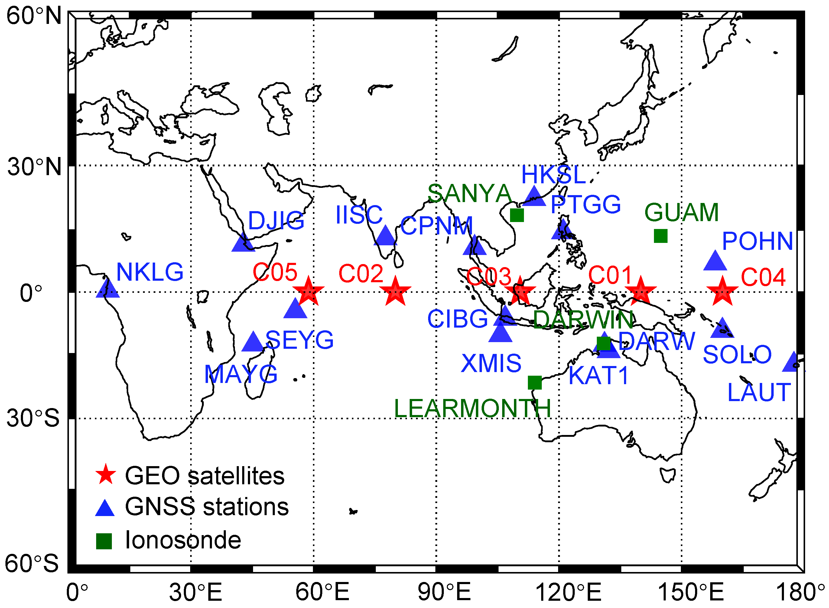
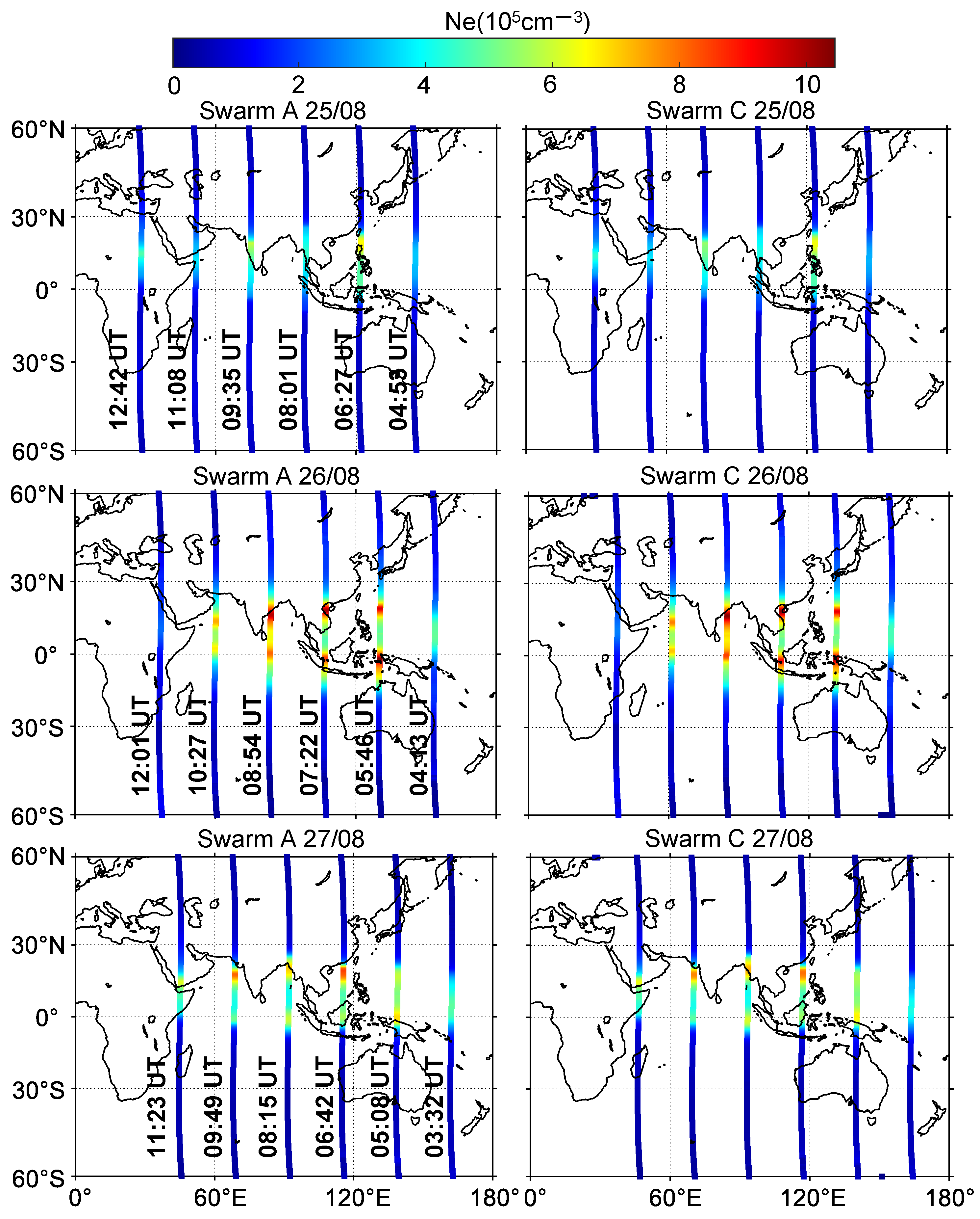
To detect ionospheric disturbance responses in TEC measurements of BDS-GEO satellites, a descriptive statistical analysis method is used on daily hourly TEC. Liu et al. [48] have first examined the ionospheric TEC observations from GPS receivers in Taiwan regions to study ionospheric electron density variations during the Chi-Chi earthquake. They have further computed a 15-day running median of the TEC and the associated inter-quartile range as a reference for detecting abnormal signals during severe earthquakes. It has demonstrated that a statistical analysis method is useful to register pre-earthquake ionospheric anomalies before significant earthquakes. Then, many researchers have started to use GPS TEC from the global ionospheric maps to statistically analyze the ionospheric disturbance responses before worldwide earthquakes [49,50,51,52,53,54]. In this work, the median of 30 days before the observed day is calculated to construct the anomaly bounds. In Equation (3), the first and third quartiles are also calculated to quantify the anomalous disturbance responses. There is a positive (greater than upper bound) or negative (smaller than lower bound) disturbance response when the value of BDS-GEO TEC is outside of the upper and lower bounds.
{ TEC i > Upper   Bound = M + 1.5 ( U Q M ) TEC i < Lower   Bound = M 1.5 ( M L Q )   positive   negative response response
where M is the median of TEC series from global ionospheric map (GIM) model; and L Q and U Q are the first and third quartiles, respectively.
The critical frequency ( f o F 2 ) and peak height ( h m F 2 ) of the ionospheric F2 layer are collected from four ionosonde stations over low-latitude regions to investigate the ionospheric disturbance responses during the different stages of the storm. Meanwhile, the relative deviations of the f o F 2 and h m F 2 are used to measure the disturbance intensity of F2 layer signatures, which is defined by equation D f o F 2 = ( f o F 2 ( i ) f o F 2 ( q ) ) / f o F 2 ( q ) and D h m F 2 = ( h m F 2 ( i ) h m F 2 ( q ) ) / h m F 2 ( q ) , where f o F 2 ( i ) and h m F 2 ( i ) represent the measurement of f o F 2 and h m F 2 during the storm time, respectively; and f o F 2 ( q ) and h m F 2 ( q ) represent the quiet value of f o F 2 and h m F 2 calculated from the five-day average before the storm, respectively. It can be considered that positive deviation corresponds to the positive ionospheric responses, and negative deviation corresponds to the negative ionospheric responses.

4. Data Sources

We use 15 multi-GNSS experiment (MGEX) stations with BDS-GEO observations and four ionosonde stations over low-latitude areas to study temporal-spatial variation of the ionosphere during the geomagnetic storm on 25–27 August 2018. Table 1 shows the detailed geographic and geomagnetic coordinates of MGEX stations. In addition, the specific locations of these stations are marked by blue triangles and green squares in Figure 1. As shown in Figure 1, the MGEX stations are distributed in latitude from 30°S to 30°N, and longitude from 0°E to 180°E. The ionosonde stations are located at 18.3°N and 109.4°E (SANYA), 13.6°N and 144.9°E (GUAM), 12.4°S and 130.9°E (DARWIN), and 21.8°S and 114.1°E (LEARMONTH), respectively. The standard GIMs are used to construct the upper and lower bounds for studying the ionospheric disturbance responses. Moreover, the solar wind velocity, F10.7 solar flux index, the interplanetary magnetic field (IMF) Bz, By, and geomagnetic indexes Dst and Kp are used to analyze the different performance of geomagnetic conditions.

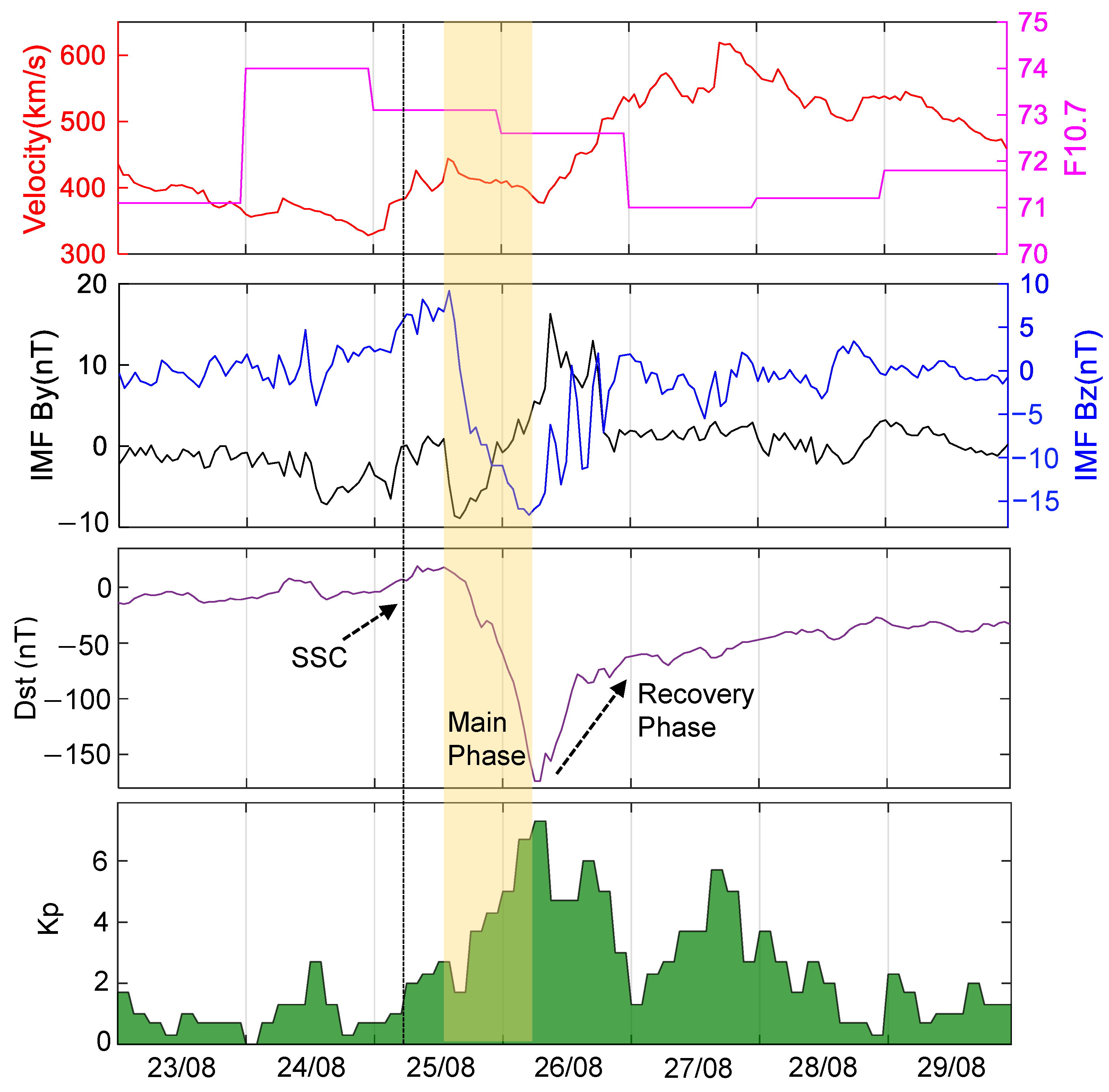
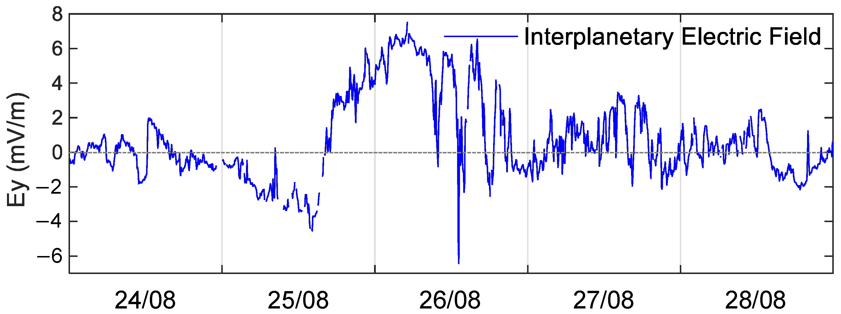
5. Solar and Geomagnetic Conditions of the Storm

In Figure 2, the solar wind velocity, F10.7 solar flux index, the interplanetary magnetic field (IMF) Bz, By, and geomagnetic parameters Dst and Kp are used to reflect the variation of geomagnetic condition during 23–29 August 2018. It can be seen that the indices IMF Bz, By, Dst and Kp all show a regular variation during 23–24 August. However, the F10.7 index shows a sudden increase to the peak value of 74 and the solar wind velocity presents a slight decrease on 24 August. The Dst index suddenly changes at 06:00 UT and then rises to 19 nT at 08:00 UT on 25 August 2018, which remains at a stable variation of around 5 to 20 nT until 16:00 UT. The geomagnetic storm sudden commencement (SSC) starts at 06:00 and lasts for 10 h. From the beginning of 17:00 UT on 25 August 2018, the Dst index decreases rapidly and reaches the minimum of −174 nT at 07:00 UT on 26 August 2018, while the Kp index reaches the maximum of nearly 7. This indicates that a strong geomagnetic storm has occurred. The main phase of the storm lasts for 14 h from 17:00 UT on 25 August to 07:00 UT on 26 August. During the main phase, the IMF Bz and By both show a disturbance that the magnitude of Bz drops from the maximum of 9 nT to the minimum of −16.8 nT, and By index increases to the peak value of nearly 15 nT. After 07:00 UT on 26 August 2018, the recovery phase of the storm lasts for about three days, shown in Figure 2. During the recovery phase, the Dst index increases gradually and returns to normal state. However, the solar wind velocity unexpectedly increases from 372 km/s to 580 km/s, as well as the IMF Bz, which is an unusual phenomenon compared with previous geomagnetic storms. The Kp index shows a peak value of 5 and then gradually decreased to quiet state during the recovery phase. During 28–29 August, all indices return to regular variation, except the solar wind velocity shows a decrease.

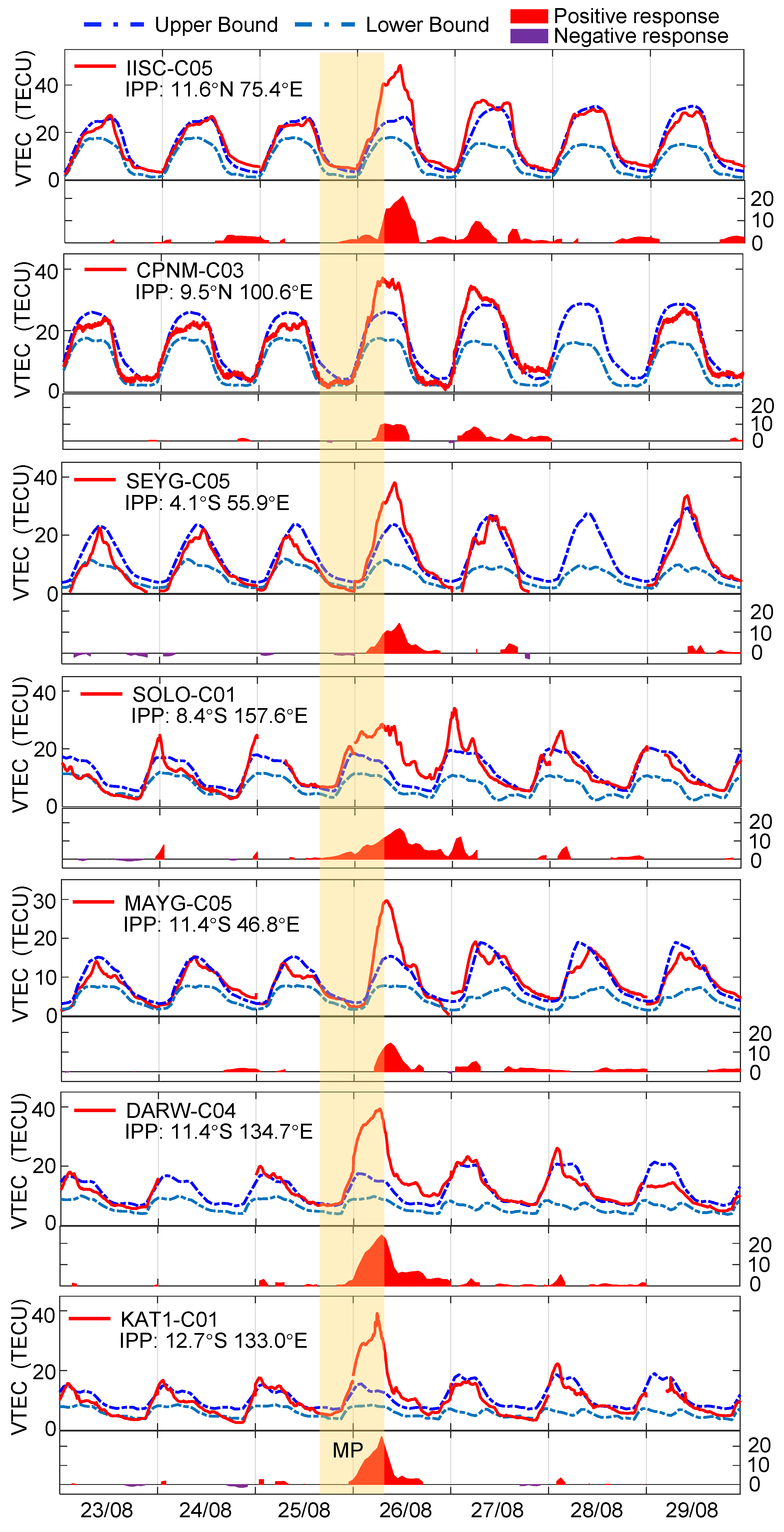
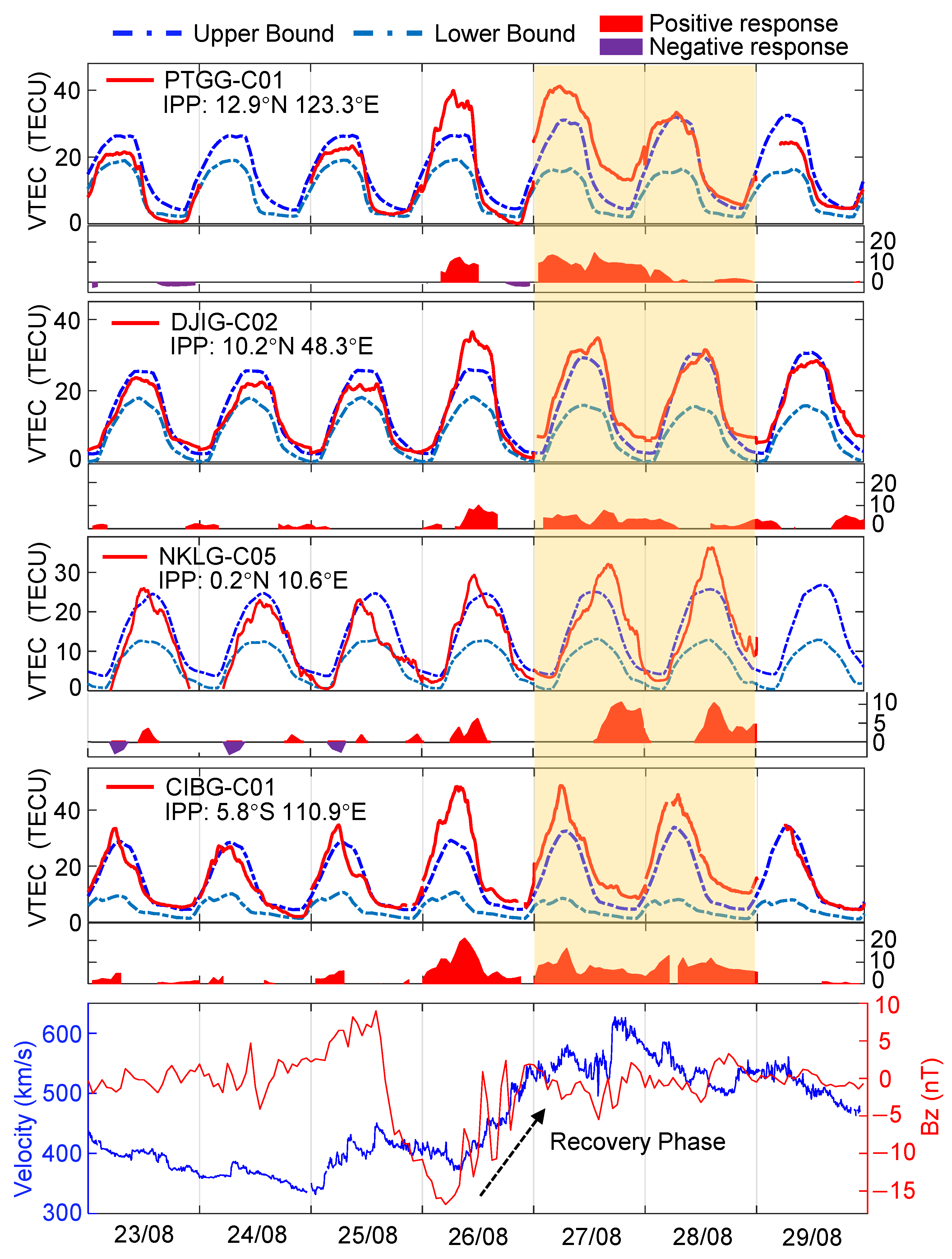
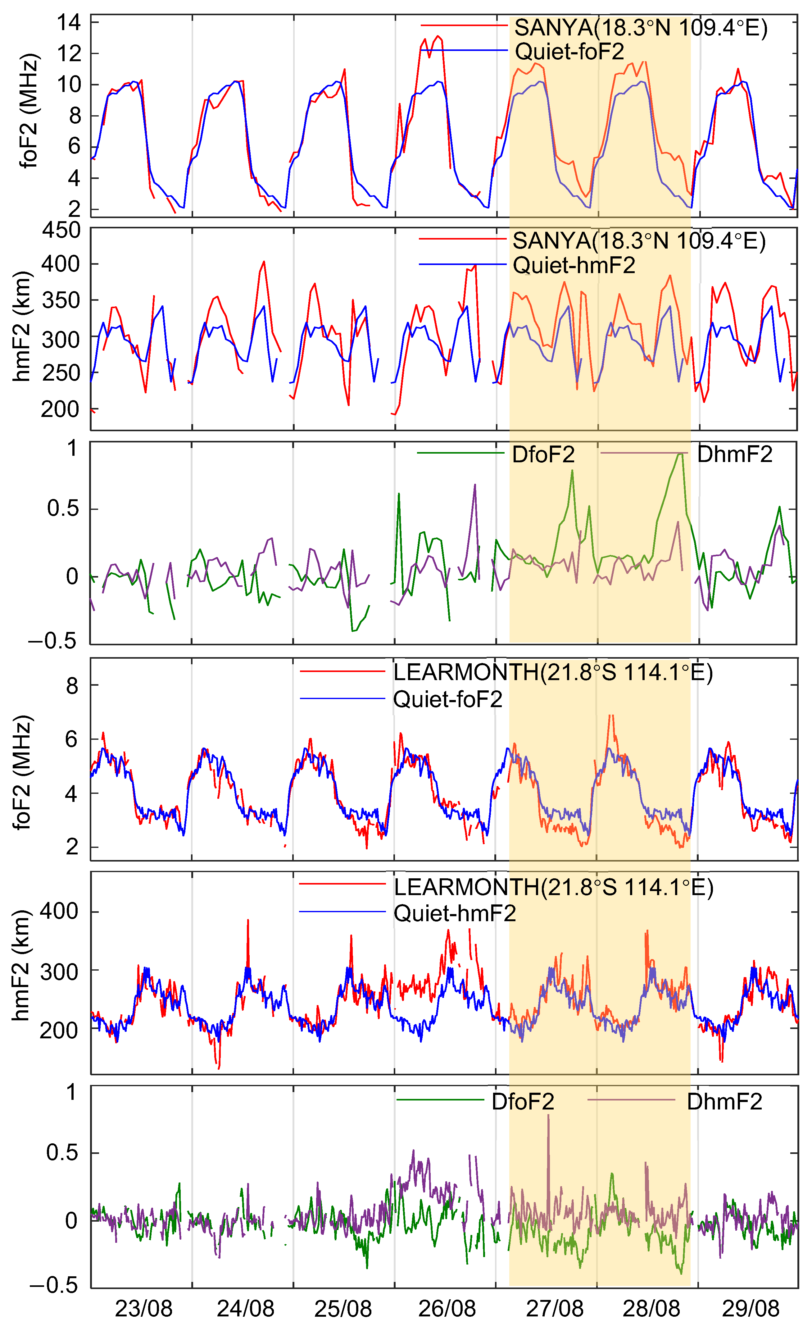
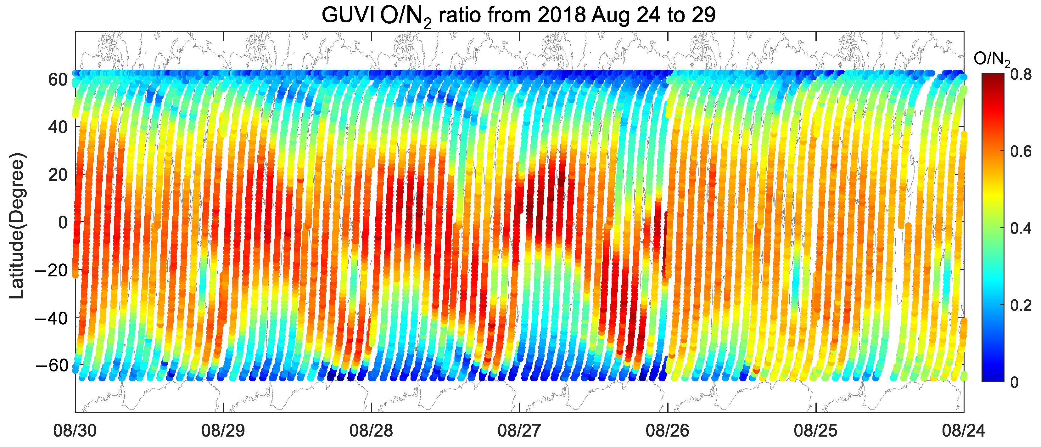
6. Ionospheric Disturbance Responses

The ionospheric responses to the geomagnetic storm on 23–29 August 2018 are investigated by BDS GEO observations. The diurnal variations of GEO TEC and the corresponding upper bounds and lower bounds are calculated from the GIM model over different locations in Figure 3. The dark blue and light blue dotted lines indicate the corresponding upper bound and lower bound, respectively. The red and purple error areas represent positive and negative disturbance signatures, respectively. The yellow area is the main phase of the storm. As shown in Figure 3, there are no significant disturbance signatures of GEO TEC during quiet time on 23–24 August 2018. The TEC magnitudes during this quiet time are 25 TECU (IISC), 20 TECU (DARW), 21 TECU (SEYG), 15 TECU (MAYG), and 18 TECU (KAT1), respectively. From the beginning of the main phase of the storm on 25 August 2018, the TEC does not immediately respond to the sudden disturbance of the geomagnetic storm. After 6 to 9 h, the magnitude of GEO TEC starts to increase rapidly. The ionospheric TEC from GEO satellites responds severely to the storm. At about 07:00–09:00 UT on 26 August 2018, the magnitudes of GEO TEC from different stations increases to the maximum of 48.2 TECU (IISC), 39.3 TECU (DARW), 38.0 TECU (SEYG), 29.6 TECU (MAYG), and 39.0 TECU (KAT1), respectively. Compared with quiet time, the relative increase from these stations is ranging from 0.8 to 1.16. The red areas show that large positive disturbance signatures of low-latitude ionosphere are detected during the main phase of the storm. The largest positive response is up to about 25.1 TECU at KAT1 station, and the smallest is up to 14.1 TECU at MAYG station. As the recovery phase starting on 26 August 2018, the magnitude of GEO TEC decreases to normal state, and the intensity of positive disturbance signatures gradually weaken, which indicates the local ionosphere observed from these stations returns to quiet state during the recovery phase.
Figure 4 shows the variation of critical frequency ( f o F 2 ) and peak height ( h m F 2 ), as well their relative deviations from 23–29 August 2018 at DARWIN and GUAM stations. The peak height of F layer is often used to study the possible driving force of an electrodynamic source to uplift or decrease the ionospheric F layer. In Figure 4, the f o F 2 observed from DARWIN and GUAM stations shows an obvious enhancement up to nearly 10 MHz on 26–27 August 2018. The D f o F 2 of both two stations even increases to around 0.6–0.8, which indicates that the ionosphere generates a positive disturbance response during the main phase of the geomagnetic storm in August 2018. The h m F 2 of DARWIN station has the same trends with f o F 2 , with an increase to 380 km on 26 August. During the recovery phase of the storm, the f o F 2 and h m F 2 of two ionosonde stations have no prominent disturbance compared with the averaged quiet days.
We discover a special local-area anomaly of the low-latitude ionosphere during the recovery phase of this geomagnetic storm on 27–28 August 2018. Figure 5 shows the variation of GEO TEC and the corresponding disturbance bounds from four stations during 23–29 August 2018. It can be seen that the GEO TEC started to exceed the upper bound at around 02:00 UT on 27 August. The positive disturbance signatures occur, and the duration of signatures is up to about 1.5 days. It is noticeable that the positive response from station CIBG lasted for about 2 days. The magnitude of the GEO TEC series reaches the maximum of 41.1 TECU (PTGG), 34.8 TECU (DJIG), 35 TECU (NKLG), and 48.6 TECU (CIBG), respectively, and the corresponding positive signatures vary from 7.9 TECU to 16.3 TECU during the recovery phase on 27–29 August. Compared with the main phase of the storm, there is a long-term TEC enhancement and the duration of positive response in the recovery phase is almost 2–3 times that of the main phase. The magnitude of positive response during the recovery phase is smaller than that of the main phase. The bottom subgraph of Figure 5 represents the variation of solar wind velocity and IMF-Bz on 23–29 August 2018. It shows that there is an intensive increment on solar wind velocity, along with a moderate perturbation of IMF-Bz during the recovery phase of the storm.
The results from Figure 3, Figure 4 and Figure 5 show that a prominent positive disturbance response of the ionosphere is detected during the main phase of the storm on 26 August 2018. The magnitudes of positive signatures over all the selected stations vary from 14.1–25.1 TECU, which shows that BDS-GEO satellites can effectively detect the fine variations of ionospheric TEC. Meanwhile, the f o F 2 and h m F 2 parameters of the F2 layer also display an increment during the main phase. GEO TEC observed from four stations generate a persistent enhancement along with long-duration positive disturbance signatures on 27–29 August, which is distinct from normal performance during the recovery phase of other storms. In addition, the unique phenomenon does not cover all low-latitude areas in this paper, but exhibits a local-area characteristic, compared with similar studies on this geomagnetic storm [37,55]. Therefore, we have selected the SANYA and LEARMONTH ionosonde stations that are close to the CIBG station in the longitude direction to further investigate the performance of the ionospheric F layer during the recovery phase of the storm on 27–29 August 2018. Figure 6 shows the variation of f o F 2 and h m F 2 parameters at SANYA and LEARMONTH stations on 23–29 August. It shows that a persistently enhanced peak height up to 400 km of the F2 layer on 27–29 August is observed from two ionosonde stations. The previous studies show that the sudden increment in the layer height of the ionosphere is likely to cause the Rayleigh-Taylor instability and the development of spread-F irregularities [40]. Combined with ionosonde results, we think that the uplift of F layer height is one of the possible factors contributing to the local-area positive disturbance signatures over low-latitude regions during the recovery phase of this storm.
Figure 7 presents the variations of the electron density Ne observed from the Swarm A and C satellites on 25–27 August 2018. The Ne is regarded as the regular level reference to analyze the disturbed variation of Ne from Swarm A and C during the storm time on 25 August. It can notice that the variation of low-latitude Ne from Swarm A and C both present a strong equatorial ionization anomaly (EIA) crest from 60°E to 130°E during the main phase of storm on 26 August. The uplift of ionospheric F2 layer observed from ionosonde SANYA is simultaneous with this strong EIA crest. The intensity of EIA crest magnitude on August 27 has become smaller than that of EIA crest magnitude on 26 August, but along with an obvious enhancement of Ne over low-latitude areas compared to the Ne on 25 August. The in situ electron density Ne measured by the Swarm A and C satellites verifies the presence of the persistent positive response and the uplift of F2 layer observed from GEO satellites and ionosonde stations during this geomagnetic storm.

7. Discussion

The change of thermospheric composition is often regarded as one of the sources causing the global ionospheric disturbances, and the O/N2 ratio is used as an important index of thermospheric composition to investigate the ionospheric disturbance responses during geomagnetic storms [56]. Paul et al. [57] used the TEC data derived from the GPS receivers to investigate the latitudinal ionospheric response of three geomagnetic storms, and found that the enhancement of O/N2 ratio possibly contributed to the positive disturbance signatures of the storm during the recovery phase. Bagiya et al. [58] proposed that the production or enhancement of ionospheric plasma at F region heights is attributed to the enhancement in atomic oxygen, which can explain the enhancement in O/N2 ratio at low-latitude regions. To observe the variation of thermosphere neutral composition during 24–29 August 2018, the O/N2 ratio variation is collected from Global Ultraviolet Imager (GUVI) instrument onboard the TIMED satellite. The variation of O/N2 ratio is presented in Figure 8. The O/N2 ratio is about 0.4–0.6 at quiet time on 24–25 August 2018. Compared with the value of O/N2 ratio at quiet time, the O/N2 ratio shows a prominent enhancement to nearly 1.0 at equatorial and low latitudes at 0–10 UT on 26 August 2018. During the recovery phase of the storm on 27–28 August, the O/N2 ratio also remains at high values compared with that on 24 August. Compared with other low latitudes, the areas that have a higher enhancement of O/N2 ratio are close to the locations of CIBG station and SANYA and LEARMONTH ionosondes in the longitude direction, where a persistent positive disturbance response is observed during the recovery phase of the storm. We further think that the TEC enhancement over low-latitude areas with a higher O/N2 ratio might contribute to the EIA anomaly, disturbed neutral composition, and equatorward winds [37].
The variation of interplanetary electric field during 24–28 August 2018 is presented in Figure 9, which can be controlled by the combination of high-speed solar wind and IMF Bz. As shown in Figure 9, the interplanetary electric field displays the long-duration positive phases during the recovery phase of the storm. Previous studies have demonstrated that the persistent prompt penetration of interplanetary electric field (PPEF) into the low latitudes can be attributed to the combined effects of high-speed solar wind and IMF Bz fluctuations [39]. Therefore, the enhancement of electric field caused by solar wind and IMF Bz in the low altitudes during the recovery phase of the storm possibly contributes the positive ionospheric response. The neutral winds and PPEF both result in the positive ionospheric response due to the expansion of EIA crest to higher latitudes from Figure 7 [55,59]. Additionally, the solar wind variation also can facilitate the response of O/N2 ratios during the geomagnetic storms [60]. From these results, the uplift of F layer height and the enhanced O/N2 ratio are possibly the main factors causing the local-area positive disturbance signatures over low latitudes during the recovery phase of the storm in August 2018.

8. Conclusions

We use the BDS-GEO satellites and ionosondes to investigate the disturbance responses of the low-latitude ionosphere in the eastern hemisphere during the geomagnetic storm in August 2018. The upper and lower bounds are calculated by GIM TEC to detect the positive or negative signatures from the BDS GEO TEC. The BDS GEO satellites can effectively detect the high-resolution variations of ionospheric TEC, compared with the GIM model during the long-term monitoring. During the main phase of the storm, the large positive disturbance signatures are detected on 26 August over all the selected stations at low-latitude regions, and the magnitude of disturbance signatures vary from 14.1 to 25.1 TECU. During the recovery phase of the storm, the local persistent positive signatures are observed on 27–28 August. The increment of f o F 2 and h m F 2 are also observed by using ionosondes. The in situ electron density Ne measured by the Swarm A and C satellites also verifies the presence of the uplift of the F2 layer observed from ionosonde stations during this geomagnetic storm. The thermospheric composition variation possibly has a direct impact on the disturbance responses of ionospheric TEC. The positive disturbance signatures at low latitudes during the recovery phases of the storm are mainly attributed to the enhancement of the O/N2 ratio and the uplift of the F layer.

Author Contributions

J.T. and X.G. conceived and designed the experiments; J.T. and X.G. performed the experiments; X.G. and Z.Z. wrote the paper; D.Y. and X.H. analyzed the data; J.T. and X.W. revised the paper. All authors have read and agreed to the published version of the manuscript.

Funding

This research is supported by the National Key Research & Development Program (No. 2017YFE0131400), the National Natural Science Foundation of China (No. 42074045), the Key Laboratory for Digital Land and Resources of Jiangxi Province, East China University of Technology (No. DLLJ202104), and the National Natural Science Foundation of China (No. 41761089).

Institutional Review Board Statement

Not applicable.

Informed Consent Statement

Not applicable.

Data Availability Statement

MGEX data are available from https://cddis.nasa.gov/archive/gnss/data/campaign/mgex/ (accessed on 12 August 2021). The ionosondes data are provided by GIRODidbase (https://ulcar.uml.edu/ accessed on 12 August 2021). The SANYA ionosonde data are provided by the Beijing National Observatory of Space Environment, Institute of Geology and Geophysics Chinese Academy of Sciences through the Geophysics center, National Earth System Science Data Center (http://wdc.geophys.ac.cn/ accessed on 12 August 2021). The Swarm satellite data are obtained from the European Space Agency (https://swarm-diss.eo.esa.int/ accessed on 12 August 2021). The O/N2 ratio data from GUVI are provided by the website (http://guvitimed.jhuapl.edu/ accessed on 12 August 2021). The OMNI data are obtained from the GSFC/SPDF OMNIWeb interface (http://omniweb.gsfc.nasa.gov/ accessed on 12 August 2021).

Acknowledgments

The authors acknowledge IGS for providing MGEX data, GIRODidbase for providing ionosonde data, the European Space Agency for providing Swarm satellite data, GUVI for providing O/N2 ratio data, and OMNIWeb for providing OMNI data. They would also like to thank the anonymous reviewers for their constructive comments in improving the article.

Conflicts of Interest

The authors declare no conflict of interest.

References

  1. Gonzalez, W.D.; Joselyn, J.A.; Kamide, Y.; Kroehl, H.W.; Rostoker, G.; Tsurutani, B.T.; Vasyliunas, V.M. What is a geomagnetic storm? J. Geophys. Res. Space Phys. 1994, 99, 5771–5792. [Google Scholar] [CrossRef]
  2. Cai, X.; Burns, A.G.; Wang, W.; Qian, L.; Solomon, S.C.; Eastes, R.W.; McClintock, W.E.; Laskar, F.I. Investigation of a neutral “tongue” observed by GOLD during the geomagnetic storm on May 11, 2019. J. Geophys. Res. Space Phys. 2021, 126, e2020JA028817. [Google Scholar] [CrossRef]
  3. Yue, X.; Wang, W.; Lei, J.; Burns, A.; Zhang, Y.; Wan, W.; Liu, L.; Hu, L.; Zhao, B.; Schreiner, W.S. Long-lasting negative ionospheric storm effects in low and middle latitudes during the recovery phase of the 17 March 2013 geomagnetic storm. J. Geophys. Res. Space Phys. 2016, 121, 9234–9249. [Google Scholar] [CrossRef] [Green Version]
  4. Matsushita, S. A study of the morphology of ionospheric storms. J. Geophys. Res. 1959, 64, 305–321. [Google Scholar] [CrossRef]
  5. Afraimovich, E.L.; Astafyeva, E.I.; Demyanov, V.V.; Edemskiy, I.K.; Gavrilyuk, N.S.; Ishin, A.B.; Kosogorov, E.A.; Leonovich, L.A.; Lesyuta, O.S.; Palamartchouk, K.S.; et al. A review of GPS/GLONASS studies of the ionospheric response to natural and anthropogenic processes and phenomena. J. Space Weather Space Clim. 2013, 3, A27. [Google Scholar] [CrossRef] [Green Version]
  6. Muella, M.; Paula, E.R.; Monteiro, A.A. Ionospheric scintillation and dynamics of fresnel-scale irregularities in the inner region of the equatorial ionization anomaly. Surv. Geophys. 2013, 34, 233–251. [Google Scholar] [CrossRef]
  7. Tesema, F.; Damtie, B.; Nigussie, M. The response of the ionosphere to intense geomagnetic storms in 2012 using GPS-TEC data from east Africa longitudinal sector. J. Atmos. Sol.-Terr. Phys. 2015, 135, 143–151. [Google Scholar] [CrossRef]
  8. Wen, D.; Yuan, Y.; Ou, J.; Zhang, K. Ionospheric response to the geomagnetic storm on August 21, 2003 over China using GNSS-based tomographic technique. IEEE Trans. Geosci. Remote Sens. 2010, 48, 3212–3217. [Google Scholar] [CrossRef]
  9. Huo, X.; Yuan, Y.; Ou, J.; Zhang, K. Monitoring the daytime variations of equatorial ionospheric anomaly using IONEX data and CHAMP GPS data. IEEE Trans. Geosci. Remote Sens. 2011, 49, 105–114. [Google Scholar] [CrossRef]
  10. Astafyeva, E.; Zakharenkova, I.; Förster, M. Ionospheric response to the 2015 St. Patrick’s Day storm: A global multi-instrumental overview. J. Geophys. Res. Space Phys. 2015, 120, 9023–9037. [Google Scholar] [CrossRef] [Green Version]
  11. Shults, K.; Astafyeva, E.; Adourian, S. Ionospheric detection and localization of volcano eruptions on the example of the April 2015 Calbuco events. J. Geophys. Res. Space Phys. 2016, 121, 10303–10315. [Google Scholar] [CrossRef] [Green Version]
  12. Liu, X.; Zhang, Q.; Shah, M.; Hong, Z. Atmospheric-ionospheric disturbances following the April 2015 Calbuco volcano from GPS observations. Adv. Space Res. 2017, 60, 2836–2846. [Google Scholar] [CrossRef]
  13. Savastano, G.; Komjathy, A.; Verkhoglyadova, O.; Mazzoni, A.; Crespi, M.; Wei, Y.; Mannucci, A.J. Real-time detection of tsunami ionospheric disturbances with a stand-alone GNSS receiver: A preliminary feasibility demonstration. Sci. Rep. 2017, 7, 46607. [Google Scholar] [CrossRef] [PubMed]
  14. Cherniak, I.; Zakharenkova, I. Ionospheric total electron content response to the great American solar eclipse of 21 August 2017. Geophys. Res. Lett. 2018, 45, 1199–1208. [Google Scholar] [CrossRef]
  15. Song, Q.; Ding, F.; Zhang, X.; Liu, H.; Mao, T.; Zhao, X.; Wang, Y. Medium-scale traveling ionospheric disturbances induced by Typhoon Chan-hom over China. J. Geophys. Res. Space Phys. 2019, 124, 2223–2237. [Google Scholar] [CrossRef]
  16. de Oliveira, C.; Espejo, T.; Moraes, A.; Costa, E.; Sousasantos, J.; Lourenço, L.F.D.; Abdu, M.A. Analysis of plasma bubble signatures in total electron content maps of the low-latitude ionosphere: A simplified methodology. Surv. Geophys. 2020, 41, 897–931. [Google Scholar] [CrossRef]
  17. Yadav, S.; Sunda, S.; Sridharan, R. The impact of the 17 March 2015 St. Patrick’s Day storm on the evolutionary pattern of equatorial ionization anomaly over the Indian longitudes using high-resolution spatiotemporal TEC maps: New insights. Space Weather 2016, 14, 786–801. [Google Scholar] [CrossRef]
  18. Liu, J.; Zhang, D.; Coster, A.J.; Zhang, S.R.; Ma, G.-Y.; Hao, Y.-Q.; Xiao, Z. A case study of the large-scale traveling ionospheric disturbances in the eastern Asian sector during the 2015 St. Patrick’s Day geomagnetic storm. Ann. Geophys. 2019, 37, 673–687. [Google Scholar] [CrossRef] [Green Version]
  19. Mengist, C.K. Response of ionosphere over Korea and adjacent areas to 17 March 2015 geomagnetic storm. Adv. Space Res. 2019, 64, 183–198. [Google Scholar] [CrossRef]
  20. Qian, L.; Wang, W.; Burns, A.G.; Chamberlin, P.C.; Coster, A.; Zhang, S.R.; Solomon, S.C. Solar flare and geomagnetic storm effects on the thermosphere and ionosphere during 6-11 September 2017. J. Geophys. Res. Space Phys. 2019, 124, 2298–2311. [Google Scholar] [CrossRef]
  21. Reddybattula, K.D.; Panda, S.K.; Ansari, K.; Peddi, V. Analysis of ionospheric TEC from GPS, GIM and global ionosphere models during moderate, strong, and extreme geomagnetic storms over Indian region. Acta Astronaut. 2019, 161, 283–292. [Google Scholar] [CrossRef]
  22. Zakharenkova, I.; Cherniak, I.; Krankowski, A. Features of storm-induced ionospheric irregularities from ground-based and spaceborne GPS observations during the 2015 St. Patrick’s Day storm. J. Geophys. Res. Space Phys. 2019, 124, 10728–10748. [Google Scholar] [CrossRef]
  23. Dugassa, T.; Jbhc, D.; Mn, E. Statistical study of geomagnetic storm effects on the occurrence of ionospheric irregularities over equatorial/low-latitude region of Africa from 2001 to 2017. J. Atmos. Sol.-Terr. Phys. 2020, 199, 105198. [Google Scholar] [CrossRef]
  24. Nava, B.; Rodríguez-Zuluaga, J.; Alazo-Cuartas, K.; Kashcheyev, A.; Migoya-Orué, Y.; Radicella, S.M.; Amory-Mazaudier, C.; Fleury, R. Middle- and low-latitude ionosphere response to 2015 St. Patrick’s Day geomagnetic storm. J. Geophys. Res. Space Phys. 2016, 121, 3421–3438. [Google Scholar] [CrossRef] [Green Version]
  25. Bolaji, O.S.; Adebiyi, S.J.; Fashae, J.B.; Ikubanni, S.O.; Adenle, H.A.; Owolabi, C. Pattern of latitudinal distribution of ionospheric irregularities in the African region and the effect of March 2015 St. Patrick’s Day storm. J. Geophys. Res. Space Phys. 2020, 125, e27641. [Google Scholar] [CrossRef]
  26. Sharma, S.K.; Singh, A.K.; Panda, S.K.; Ahmed, S.S. The effect of geomagnetic storms on the total electron content over the low latitude Saudi Arab region: A focus on St. Patrick’s Day storm. Astrophys. Space Sci. 2020, 365, 35. [Google Scholar] [CrossRef]
  27. Brunini, C.; Azpilicueta, F. GPS slant total electron content accuracy using the single layer model under different geomagnetic regions and ionospheric conditions. J. Geod. 2010, 84, 293–304. [Google Scholar] [CrossRef]
  28. Kunitsyn, V.; Kurbatov, G.; Yasyukevich, Y.; Padokhin, A. Investigation of SBAS L1/L5 signals and their application to the ionospheric TEC studies. IEEE Geosci. Remote Sens. Lett. 2015, 12, 547–551. [Google Scholar] [CrossRef]
  29. Zhao, X.; Jin, S.; Mekik, C.; Feng, J. Evaluation of regional ionospheric grid model over China from dense GPS observations. Geod. Geodyn. 2016, 7, 361–368. [Google Scholar] [CrossRef] [Green Version]
  30. Yang, H.; Xuhai, Y.; Zhe, Z.; Zhao, K. High-precision ionosphere monitoring using continuous measurements from BDS GEO satellites. Sensors 2018, 18, 714. [Google Scholar] [CrossRef] [Green Version]
  31. Padokhin, A.M.; Tereshin, N.A.; Yasyukevich, Y.V.; Andreeva, E.S.; Nazarenko, M.O.; Yasyukevich, A.S.; Kozlovtseva, E.A.; Kurbatov, G.A. Application of BDS-GEO for studying TEC variability in equatorial ionosphere on different time scales. Adv. Space Res. 2018, 63, 257–269. [Google Scholar] [CrossRef]
  32. Bai, X.; Cai, C. Independent temporal and spatial variation analysis of ionospheric TEC over Asia-Pacific area based on BDS GEO satellites. Meas. Sci. Technol. 2020, 31, 45004. [Google Scholar] [CrossRef]
  33. Huang, F.; Lei, J.; Otsuka, Y.; Luan, X.; Liu, Y.; Zhong, J.; Dou, X. Characteristics of medium-scale traveling ionospheric disturbances and ionospheric irregularities at mid-latitudes revealed by the total electron content associated with the Beidou geostationary satellite. IEEE Trans. Geosci. Remote Sens. 2020, 59, 6424–6430. [Google Scholar] [CrossRef]
  34. Luo, X.; Lou, Y.; Gu, S.; Li, G.; Xiong, C.; Song, W.; Zhao, Z. Local ionospheric plasma bubble revealed by BDS geostationary earth orbit satellite observations. GPS Solut. 2021, 25, 117. [Google Scholar] [CrossRef]
  35. Hu, L.; Lei, J.; Sun, W.; Zhao, X.; Wu, B.; Xie, H.; Yang, S.; Wu, Z.; Zheng, J.; Ning, B.; et al. Latitudinal variations of daytime periodic ionospheric disturbances from Beidou GEO TEC observations over China. J. Geophys. Res. Space Phys. 2021, 126, e2020JA028809. [Google Scholar] [CrossRef]
  36. Abunin, A.A.; Abunina, M.A.; Belov, A.V.; Chertok, I.M. Peculiar solar sources and geospace disturbances on 20–26 August 2018. Solar Phys. 2020, 295, 7. [Google Scholar] [CrossRef] [Green Version]
  37. Li, Q.; Huang, F.; Zhong, J.; Zhang, R.; Kuai, J.; Lei, J.; Liu, L.; Ren, D.; Ma, H.; Yoshikawa, A.; et al. Persistence of the long-duration daytime TEC enhancements at different longitudinal sectors during the August 2018 geomagnetic storm. J. Geophys. Res. Space Phys. 2020, 125, e2020JA028238. [Google Scholar] [CrossRef]
  38. Lei, J.; Huang, F.; Chen, X.; Zhong, J.; Ren, D.; Wang, W.; Yue, X.; Luan, X.; Jia, M.; Dou, X.; et al. Was magnetic storm the only driver of the long-duration enhancements of daytime total electron content in the Asian-Australian sector between 7 and 12 September 2017? J. Geophys. Res. Space Phys. 2018, 123, 3217–3232. [Google Scholar] [CrossRef]
  39. Ren, D.; Lei, J.; Zhou, S.; Li, W.; Huang, F.; Luan, X.; Dang, T.; Liu, Y. High-speed solar wind imprints on the ionosphere during the recovery phase of the August 2018 geomagnetic storm. Space Weather 2020, 18, e2020SW002480. [Google Scholar] [CrossRef]
  40. Moro, J.; Xu, J.; Denardini, C.M.; Resende, L.C.A.; Neto, P.B.; Da Silva, L.A.; Silva, R.P.; Chen, S.S.; Picanço, G.A.S.; Carmo, C.S.; et al. First look at a geomagnetic storm with Santa Maria Digisonde data: F region signatures and comparisons over the American sector. J. Geophys. Res. Space Phys. 2021, 126, e2020JA028663. [Google Scholar] [CrossRef]
  41. Blagoveshchensky, D.V.; Sergeeva, M.A. Ionospheric parameters in the European sector during the magnetic storm of August 25–26, 2018. Adv. Space Res. 2020, 65, 11–18. [Google Scholar] [CrossRef]
  42. Sardon, E.; Rius, A.; Zarraoa, N. Estimation of the transmitter and receiver differential biases and the ionospheric total electron content from Global Positioning System observations. Radio Sci. 1994, 29, 577–586. [Google Scholar] [CrossRef]
  43. Zhang, B.; Ou, J.; Yuan, Y.; Li, Z. Extraction of line-of-sight ionospheric observables from GPS data using precise point positioning. Sci. China Earth Sci. 2012, 55, 1919–1928. [Google Scholar] [CrossRef]
  44. Liu, T.; Zhang, B.; Yuan, Y.; Li, Z.; Wang, N. Multi-GNSS triple-frequency differential code bias (DCB) determination with precise point positioning (PPP). J. Geod. 2019, 93, 765–784. [Google Scholar] [CrossRef]
  45. Ciraolo, L.; Azpilicueta, F.; Brunini, C.; Meza, A.; Radicella, S.M. Calibration errors on experimental slant total electron content (TEC) determined with GPS. J. Geod. 2007, 81, 111–120. [Google Scholar] [CrossRef]
  46. Xiang, Y.; Gao, Y. Improving DCB estimation using uncombined PPP. Navigation 2017, 64, 463–473. [Google Scholar] [CrossRef]
  47. Li, Z.; Yuan, Y.; Hui, L.; Ou, J.; Huo, X. Two-step method for the determination of the differential code biases of COMPASS satellites. J. Geod. 2012, 86, 1059–1076. [Google Scholar] [CrossRef]
  48. Liu, J.Y.; Chen, Y.I.; Chuo, Y.J.; Tsai, H.F. Variations of ionospheric total electron content during the Chi-Chi earthquake. Geophys. Res. Lett. 2001, 28, 1383–1386. [Google Scholar] [CrossRef] [Green Version]
  49. Ho, Y.Y.; Jhuang, H.K.; Su, Y.C.; Liu, J.Y. Seismo-ionospheric anomalies in total electron content of the GIM and electron density of DEMETER before the 27 February 2010 M8.8 Chile Earthquake. Adv. Space Res. 2013, 51, 2309–2315. [Google Scholar] [CrossRef]
  50. Tang, J.; Yao, Y.; Zhang, L. Temporal and spatial ionospheric variations of 20 April 2013 earthquake in Yaan, China. IEEE Geosci. Remote Sens. Lett. 2015, 12, 2242–2246. [Google Scholar] [CrossRef]
  51. Jiang, W.; Ma, Y.; Zhou, X.; Li, Z.; An, X.; Wang, K. Analysis of ionospheric vertical total electron content before the 1 April 2014 Mw 8.2 Chile earthquake. J. Seismol. 2017, 21, 1599–1612. [Google Scholar] [CrossRef]
  52. Tao, D.; Cao, J.; Battiston, R.; Li, L.; Ma, Y.; Liu, W.; Zhima, Z.; Wang, L.; Dunlop, M.W. Seismo-ionospheric anomalies in ionospheric TEC and plasma density before the 17 July 2006 M7.7 south of Java earthquake. Ann. Geophys. 2017, 35, 589–598. [Google Scholar] [CrossRef] [Green Version]
  53. Shah, M.; Tariq, M.A.; Ahmad, J.; Naqvi, N.A.; Jin, S. Seismo ionospheric anomalies before the 2007 M7.7 Chile earthquake from GPS TEC and DEMETER. J. Geodyn. 2019, 127, 42–51. [Google Scholar] [CrossRef]
  54. Liu, J.Y.; Le, H.; Chen, Y.I.; Chen, C.H.; Liu, L.; Wan, W.; Su, Y.Z.; Sun, Y.Y.; Lin, C.H.; Chen, M.Q. Observations and simulations of seismoionospheric GPS total electron content anomalies before the 12 January 2010 M7 Haiti earthquake. J. Geophys. Res. Space Phys. 2011, 116, A04302. [Google Scholar] [CrossRef] [Green Version]
  55. Lissa, D.; Srinivasu, V.; Prasad, D.; Niranjan, K. Ionospheric response to the 26 August 2018 geomagnetic storm using GPS-TEC observations along 80°E and 120°E longitudes in the Asian sector. Adv. Space Res. 2020, 66, 1427–1440. [Google Scholar] [CrossRef]
  56. Mansilla, G.A.; Zossi, M.M. Effects on the equatorial and low latitude thermosphere and ionosphere during the 19–22 December 2015 geomagnetic storm period. Adv. Space Res. 2019, 65, 2083–2089. [Google Scholar] [CrossRef]
  57. Paul, B.; Kumar, D.B.; Anirban, G. Latitudinal variation of F-region ionospheric response during three strongest geomagnetic storms of 2015. Acta Geod. Geophys. 2018, 53, 579–606. [Google Scholar] [CrossRef]
  58. Bagiya, M.S.; Hazarika, R.; Laskar, F.I.; Sunda, S.; Gurubaran, S.; Chakrabarty, D.; Bhuyan, P.K.; Sridharan, R.; Veenadhari, B.; Pallamraju, D. Effects of prolonged southward interplanetary magnetic field on low-latitude ionospheric electron density. J. Geophys. Res. Space Phys. 2014, 119, 5764–5776. [Google Scholar] [CrossRef]
  59. Liu, J.; Wang, W.; Burns, A.; Solomon, S.C.; Zhang, S.; Zhang, Y.; Huang, C. Relative importance of horizontal and vertical transports to the formation of ionospheric storm-enhanced density and polar tongue of ionization. J. Geophys. Res. Space Phys. 2016, 121, 8121–8133. [Google Scholar] [CrossRef]
  60. Chen, Y.; Wang, W.; Burns, A.G.; Liu, S.; Gong, J.; Yue, X.; Jiang, G.; Coster, A. Ionospheric response to CIR-induced recurrent geomagnetic activity during the declining phase of solar cycle 23. J. Geophys. Res. Space Phys. 2015, 120, 1394–1418. [Google Scholar] [CrossRef] [Green Version]
Figure 1. Blue triangles represent locations of MGEX stations, and the green squares represent ionosonde stations. The red stars represent projections of BeiDou Navigation Satellite System Geostationary Earth Orbit (BDS-GEO) satellites on the ground.
Remotesensing 14 02272 g001
Figure 2. Temporal variations of solar wind velocity, IMF-Bz component, Dst and Kp indexes during 23–29 August 2018. The yellow shadow shows the period of the storm main phase.
Remotesensing 14 02272 g002
Figure 3. Diurnal variations of Geostationary Earth Orbit (GEO) total electron content (TEC) and corresponding upper bounds and lower bounds calculated from the global ionospheric map (GIM) model over different stations during 23–29 August 2018. The red and purple areas represent positive signatures and negative signatures, respectively. The yellow vertical bar is the duration of the main phase. The VTEC is vertical TEC, and the TECU is TEC Units.
Remotesensing 14 02272 g003
Figure 4. The f o F 2 and h m F 2 (red lines) and corresponding averaged quiet values (blue lines) at DARWIN and GUAM stations. The green and purple lines represent D f o F 2 and D h m F 2 , respectively. The yellow bars represent the duration of the main phase.
Remotesensing 14 02272 g004
Figure 5. Diurnal variations of GEO TEC and the corresponding disturbance bounds from four stations during 23–29 August 2018. The bottom figure shows the variation of solar wind velocity (blue line) and IMF-Bz (red line), respectively. The yellow bar is the disturbance duration during the recovery phase.
Remotesensing 14 02272 g005
Figure 6. The f o F 2 and h m F 2 (red lines) and corresponding averaged quiet values (blue lines) at SANYA and LEARMONTH stations. The green and purple lines represent D f o F 2 and D h m F 2 , respectively. The yellow bars represent disturbance duration during the recovery phase.
Remotesensing 14 02272 g006
Figure 7. The electron density Ne from Swarm satellites A and C on 25–27 August 2018.
Remotesensing 14 02272 g007
Figure 8. Variation of O/N2 ratio from TIMED/GUVI during 24–29 August 2018.
Remotesensing 14 02272 g008
Figure 9. Variation of the interplanetary electric field during 24–28 August 2018.
Remotesensing 14 02272 g009
Table 1. The list of geographic and geomagnetic coordinates of multi-GNSS experiment (MGEX) stations.
StationGeographic CoordinatesGeomagnetic Coordinates
CIBG6.4°S, 106.8°E15.7°S, 179.5°E
CPNM10.7°N, 99.3°E1.3°N, 172.1°E
DARW12.8°S, 131.1°E21.3°S, 155.0°W
DJIG11.5°N, 42.8°E7.2°N, 116.9°E
HKSL22.4°N, 113.9°E12.9°N, 173.7°W
IISC13.0°N, 77.6°E4.7°N, 151.0°E
KAT114.4°S, 132.2°E22.8°S, 153.7°W
LAUT17.6°S, 177.4°E20.5°S, 106.8°W
MAYG12.8°S, 45.3°E16.9°S, 115.7°E
NKLG0.4°N, 9.7°E1.6°N, 82.5°E
POHN6.9°N, 158.2°E0.8°N, 129.6°W
PTGG14.5°N, 121.0°E5.2°N, 166.7°W
SEYG4.7°S, 55.5°E10.4°S, 127.1°E
SOLO9.4°S, 159.9°E14.9°S, 125.7°W
XMIS10.5°S, 105.7°E19.8°S, 178.3°E
Publisher’s Note: MDPI stays neutral with regard to jurisdictional claims in published maps and institutional affiliations.

