
What Is the Most Suitable Height Range of ALS Point Cloud and LiDAR Metric for Understorey Analysis? A Study Case in a Mixed Deciduous Forest, Pokupsko Basin, Croatia

 , , , ,
  and
and
Abstract
:1. Introduction
- (i)
- Modelling plot-level height to canopy base (HCB) models based on LiDAR data;
- (ii)
- To test the performance of the method using understorey field data and, lastly;
- (iii)
- To analyse the influence of the HCB filter, which is used to select understorey LiDAR points, LiDAR metrics and other factors on the estimates of the UH and UC.
2. Materials and Methods
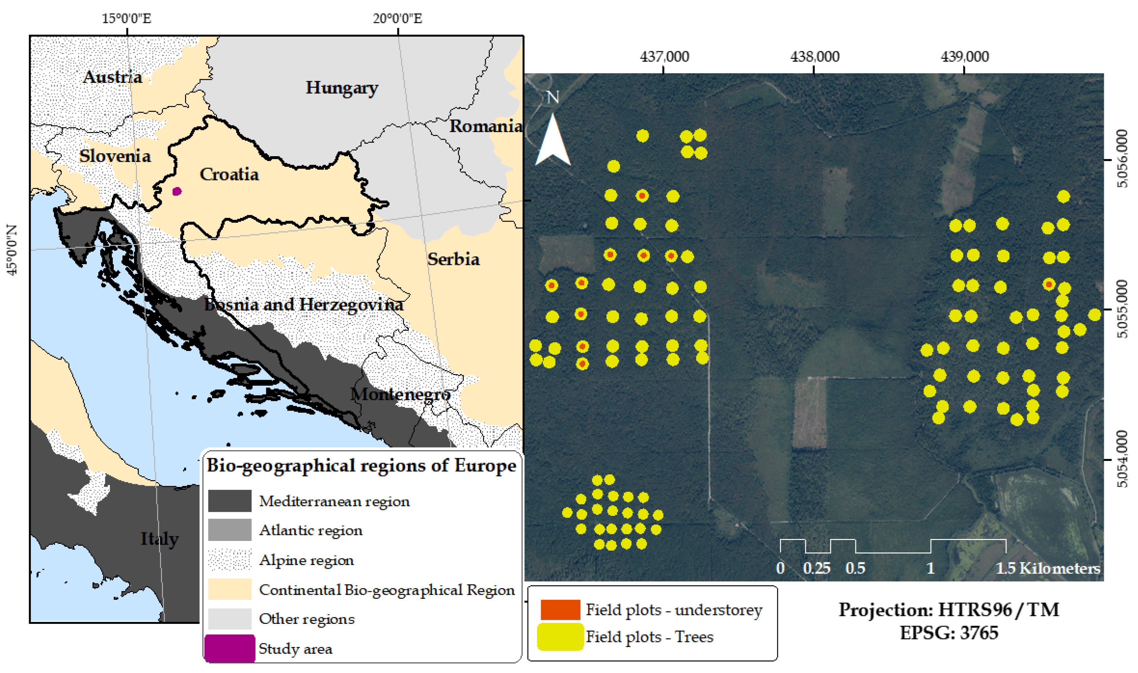
2.1. Study Area
2.2. Datasets
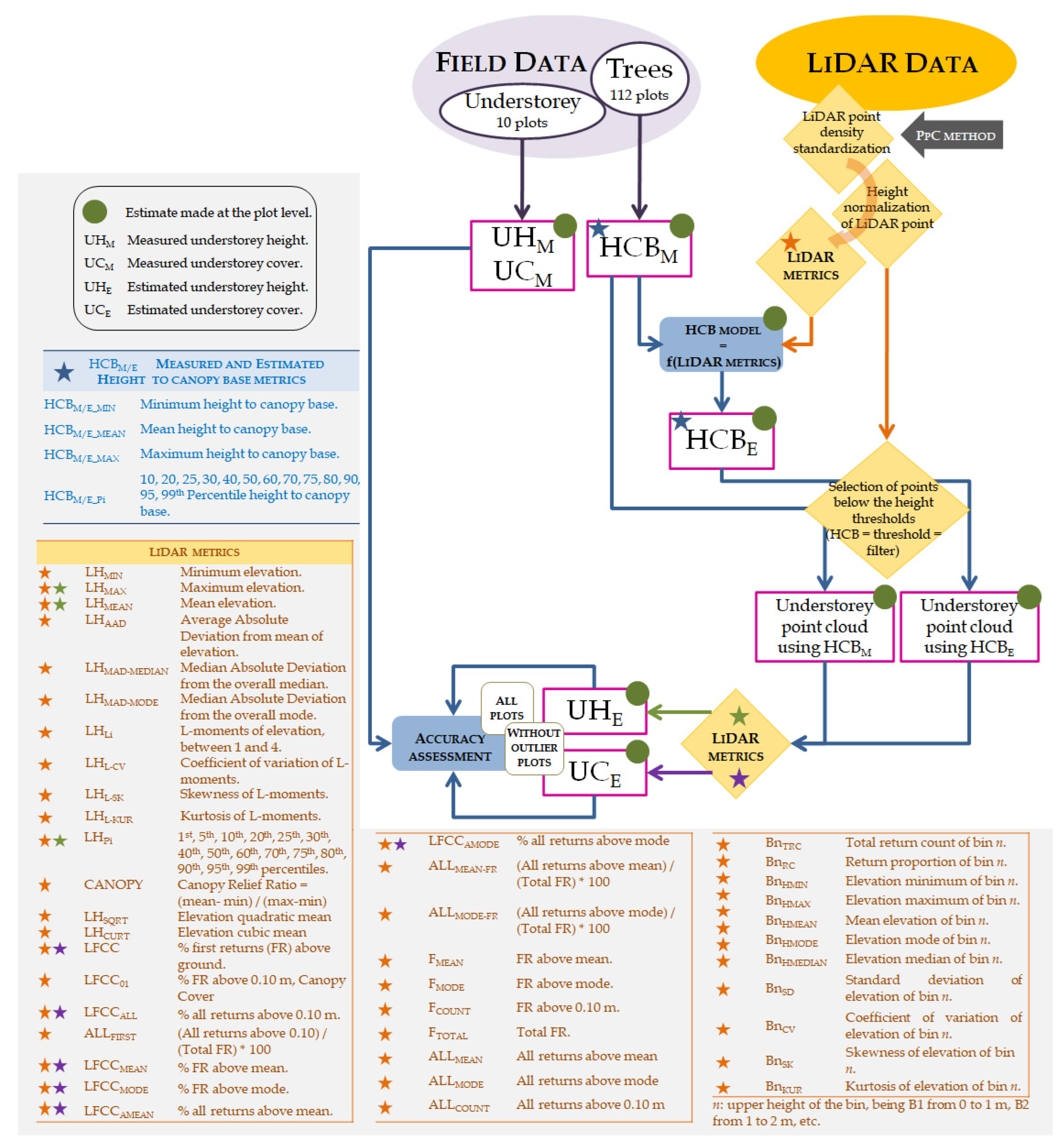
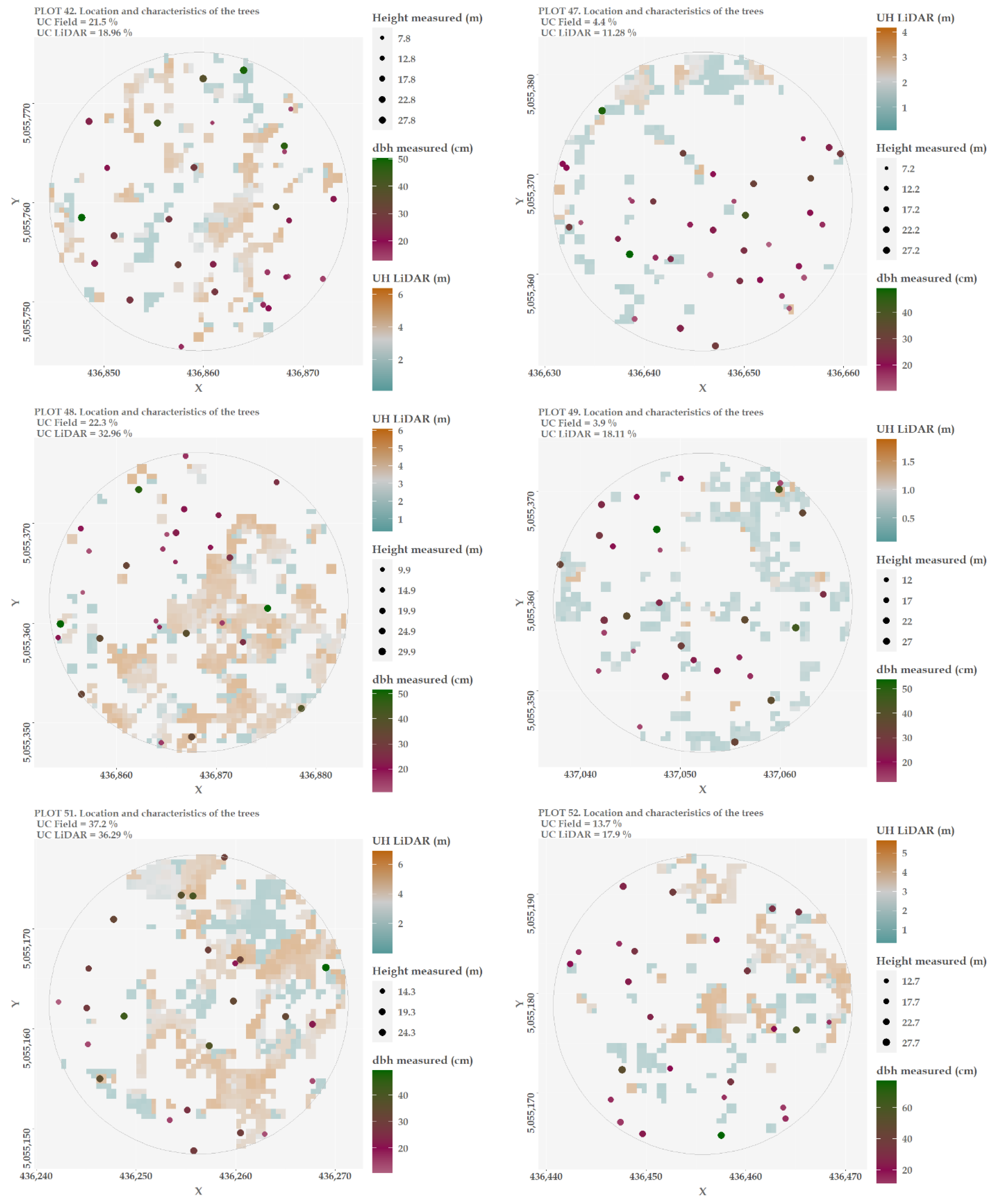
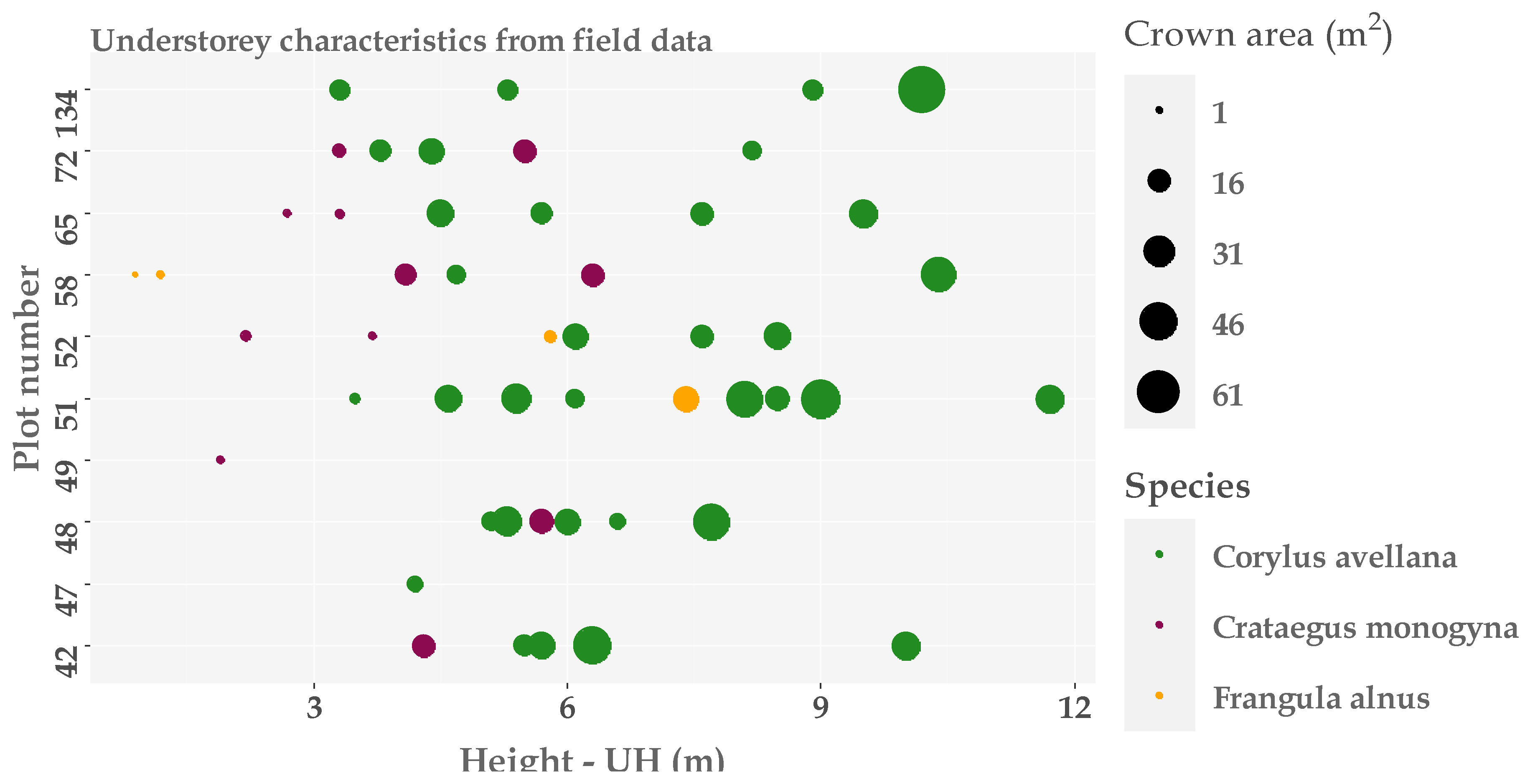
2.2.1. Field Data
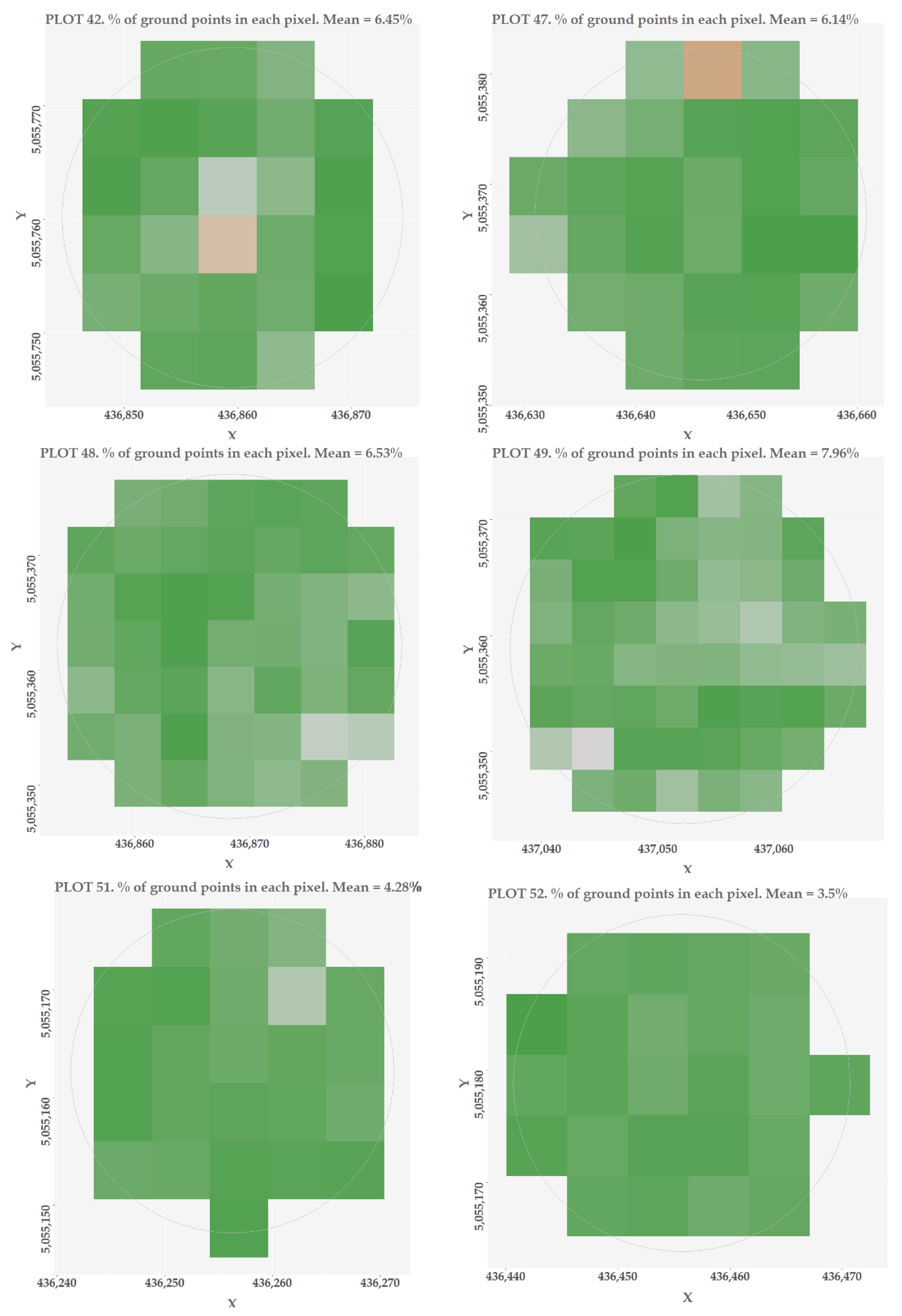
2.2.2. LiDAR Data
2.3. Methodology
2.3.1. Processing LiDAR Data
2.3.2. Estimates of HCB Models
2.3.3. Understorey Analysis and Assessment
3. Results and Discussion
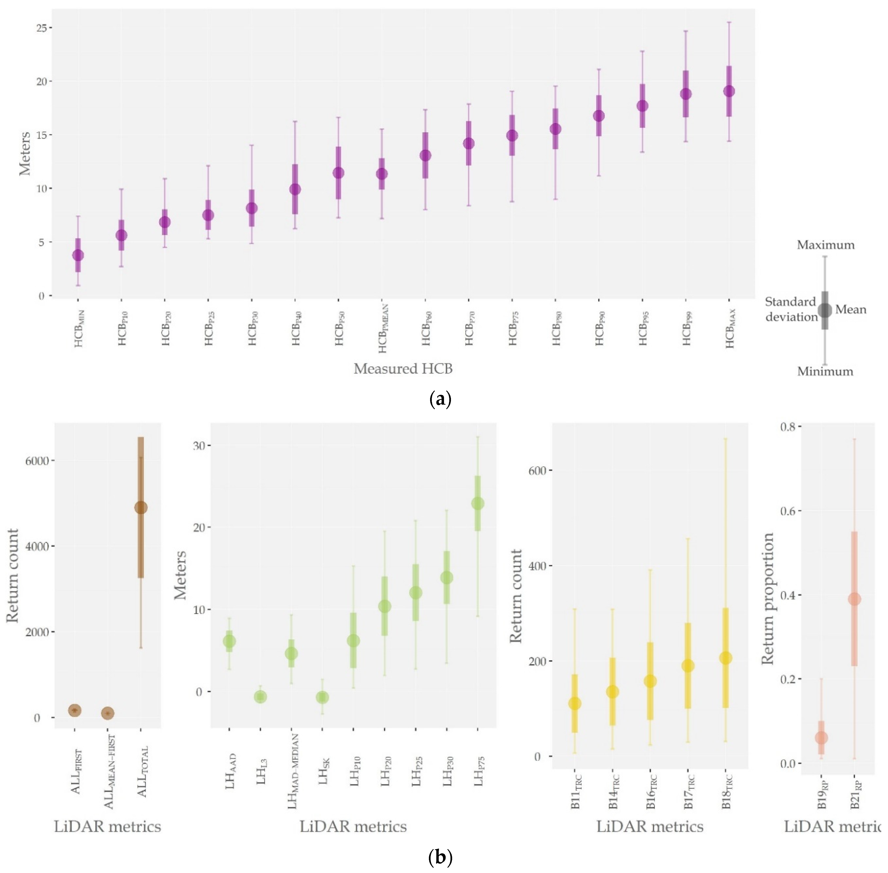
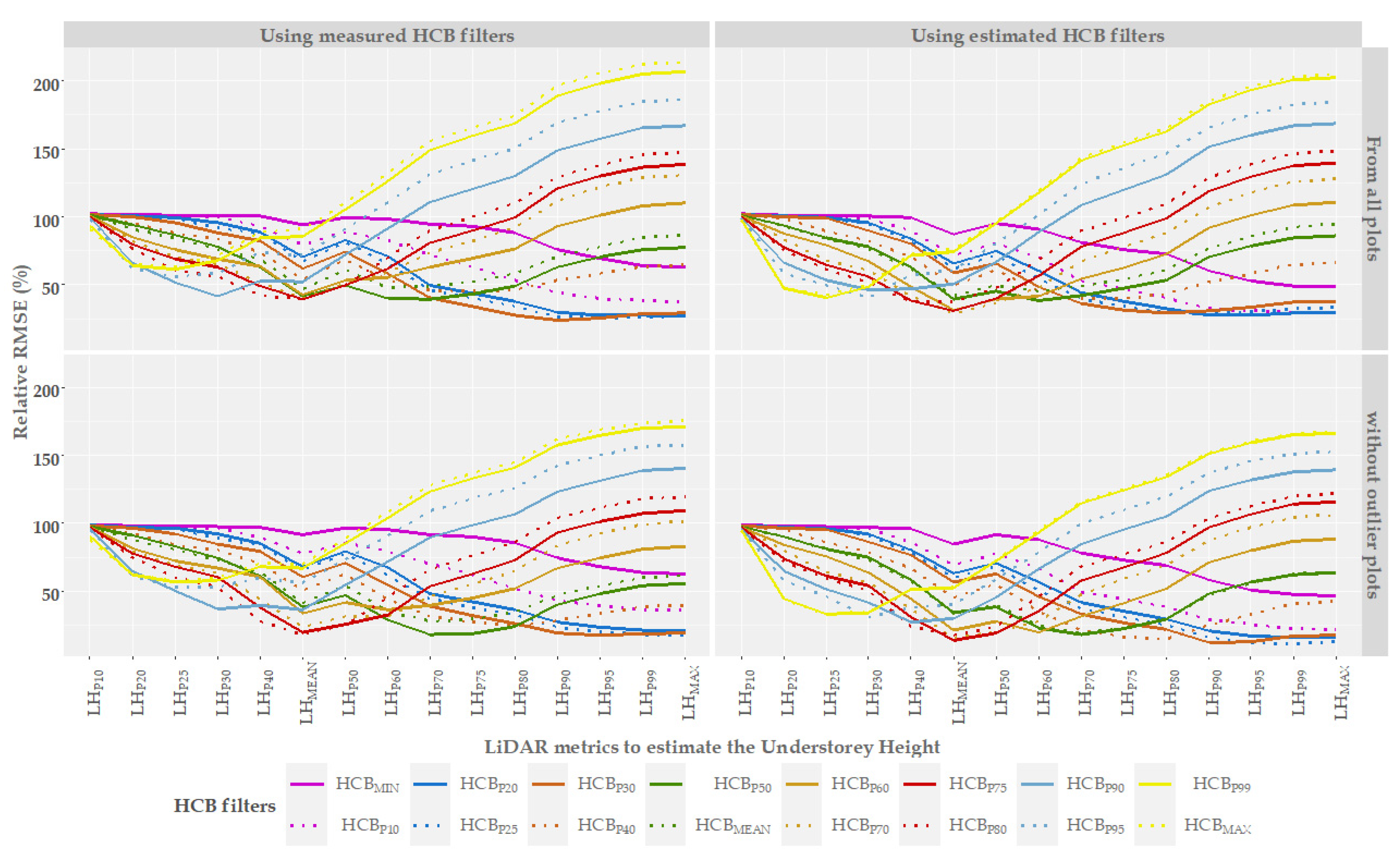
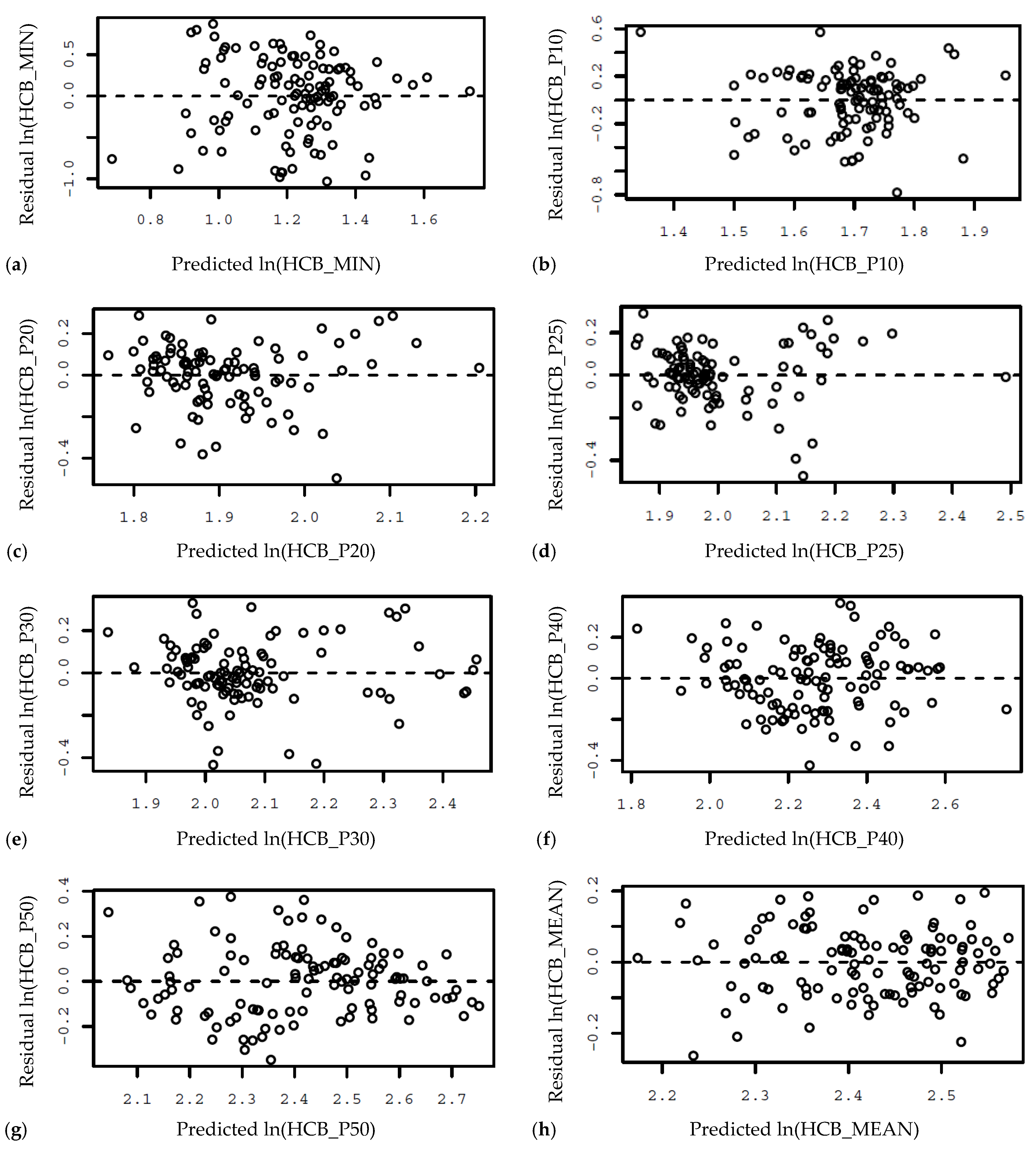
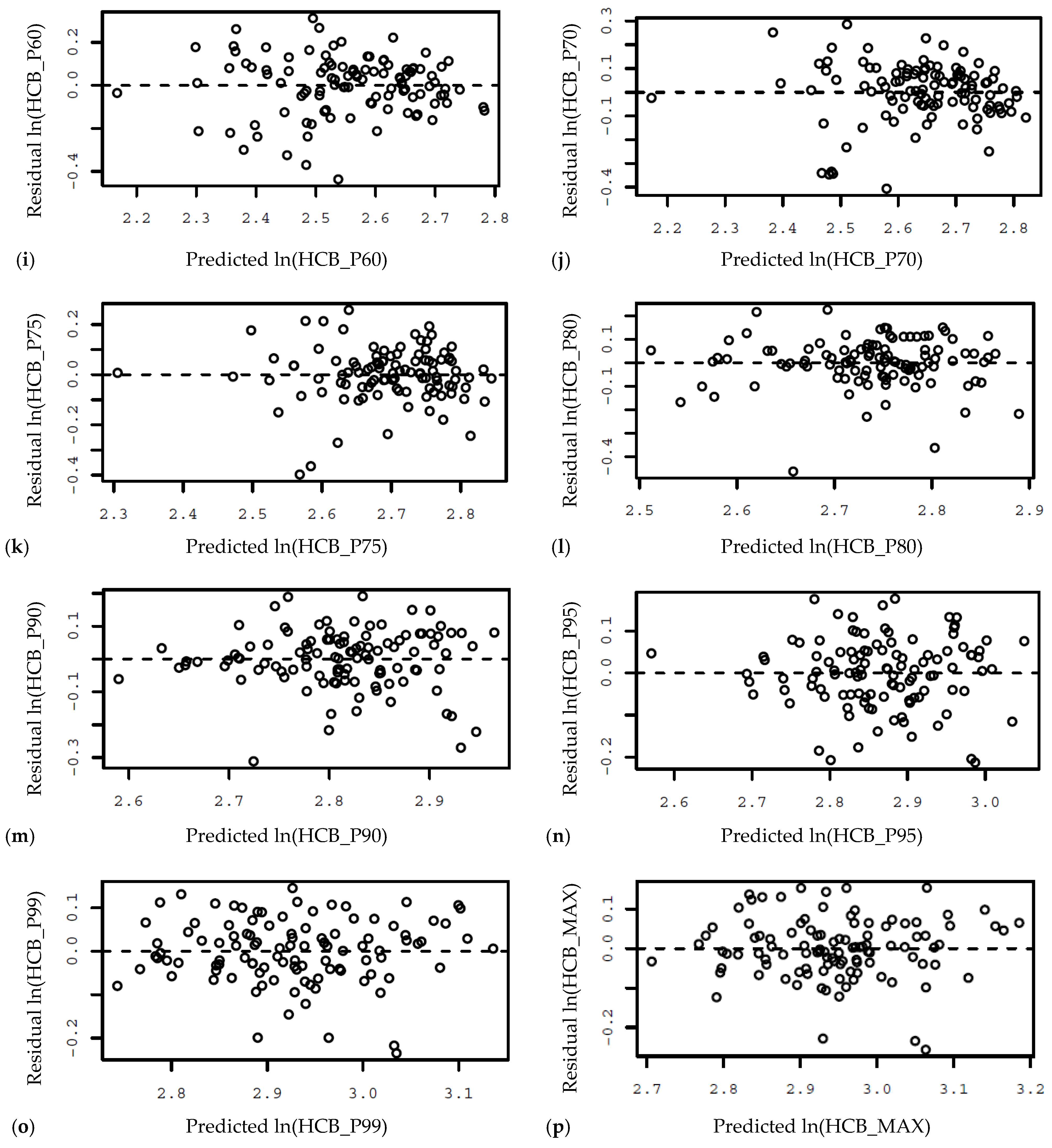
3.1. Estimates of HCB Filters
3.2. Understorey Evaluation
3.2.1. Understorey Height Evaluation
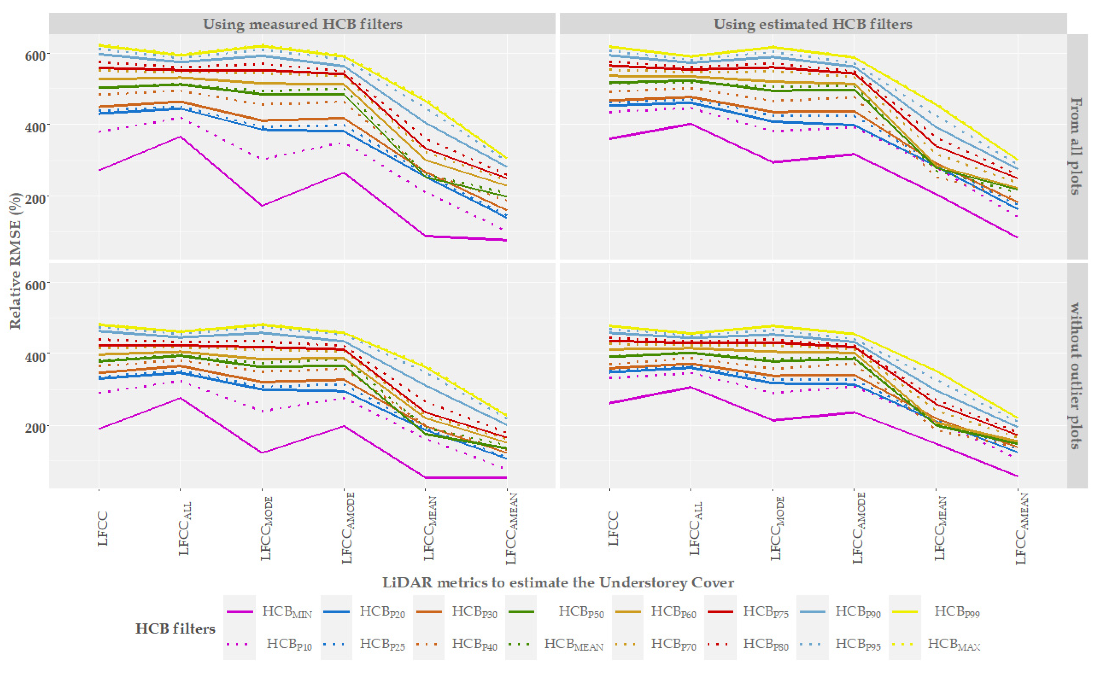
3.2.2. Understorey Cover Evaluation
3.3. Effects of Factors on the Quality of UHE and UCE
4. Conclusions
Supplementary Materials
Author Contributions
Funding
Acknowledgments
Conflicts of Interest
Abbreviations
| dbh | Diameter at breast height. |
| hcb | Individual height to crown base. |
| HCB | Height to canopy base. |
| HCBM/HCBE | Height to canopy base models using measured and estimated data, respectively. |
| UHM/UHE | Measured and estimated understorey height. |
| UCM/UCE | Measured and estimated understorey cover. |
Appendix A. Comparison between the Field Data and LiDAR Data


Appendix B. Quantitative Results

| Parameter | Mean | Min | Max | SD |
|---|---|---|---|---|
| HCBMIN | 3.75 | 0.93 | 7.39 | 1.57 |
| HCBP10 | 5.63 | 2.69 | 9.91 | 1.42 |
| HCBP20 | 6.84 | 4.48 | 10.90 | 1.19 |
| HCBP25 | 7.51 | 5.29 | 12.10 | 1.40 |
| HCBP30 | 8.14 | 4.85 | 14.02 | 1.72 |
| HCBP40 | 9.92 | 6.23 | 16.24 | 2.33 |
| HCBP50 | 11.44 | 7.24 | 16.60 | 2.45 |
| HCBMEAN | 11.35 | 7.17 | 15.51 | 1.47 |
| HCBP60 | 13.07 | 8.00 | 17.32 | 2.15 |
| HCBP70 | 14.20 | 8.39 | 17.87 | 2.08 |
| HCBP75 | 14.94 | 8.76 | 19.05 | 1.91 |
| HCBP80 | 15.55 | 8.97 | 19.54 | 1.89 |
| HCBP90 | 16.77 | 11.17 | 21.10 | 1.92 |
| HCBP95 | 17.69 | 13.38 | 22.78 | 2.06 |
| HCBP99 | 18.81 | 14.35 | 24.67 | 2.17 |
| HCBMAX | 19.07 | 14.40 | 25.50 | 2.36 |
| ALLFIRST | 162.74 | 118.13 | 193.34 | 16.89 |
| ALLMEAN−FIRST | 94.30 | 62.34 | 111.57 | 8.19 |
| ALLTOTAL | 4897.66 | 1622.00 | 6063.00 | 1647.01 |
| LHAAD | 6.11 | 2.68 | 8.90 | 1.31 |
| LHL3 | −0.67 | −1.39 | 0.68 | 0.40 |
| LHMAD−MEDIAN | 4.62 | 0.94 | 9.32 | 1.71 |
| LHSK | −0.71 | −2.77 | 1.45 | 0.52 |
| LHP10 | 6.19 | 0.39 | 15.29 | 3.39 |
| LHP20 | 10.37 | 1.93 | 19.50 | 3.62 |
| LHP25 | 12.03 | 2.73 | 20.79 | 3.47 |
| LHP30 | 13.89 | 3.42 | 22.06 | 3.24 |
| LHP75 | 22.90 | 9.15 | 31.01 | 3.37 |
| B11TRC | 110.54 | 6.00 | 309.00 | 61.27 |
| B14TRC | 135.35 | 15.00 | 308.00 | 71.21 |
| B16TRC | 157.40 | 23.00 | 391.00 | 81.40 |
| B17TRC | 189.57 | 29.00 | 456.00 | 90.07 |
| B18TRC | 206.03 | 31.00 | 666.00 | 105.10 |
| B19RP | 0.06 | 0.01 | 0.20 | 0.04 |
| B21RP | 0.39 | 0.01 | 0.77 | 0.16 |


References
- Ruiz, L.Á.; Recio, J.A.; Crespo-Peremarch, P.; Sapena, M. An Object-Based Approach for Mapping Forest Structural Types Based on Low-Density LiDAR and Multispectral Imagery Based on Low-Density LiDAR and Multispectral Imagery. Geocarto Int. 2016, 33, 443–457. [Google Scholar] [CrossRef]
- Lim, K.; Treitz, P.; Wulder, M.; St-Onge, B.; Flood, M. LiDAR Remote Sensing of Forest Structure. Prog. Phys. Geogr. 2003, 27, 88–106. [Google Scholar] [CrossRef] [Green Version]
- Crespo-Peremarch, P.; Ruiz, L.A.; Balaguer-Beser, A. A Comparative Study of Regression Methods to Predict Forest Structure and Canopy Fuel Variables from LiDAR Full-Waveform Data. Rev. De Teledetección 2016, 45, 27–40. [Google Scholar] [CrossRef] [Green Version]
- Almeida, D.R.A.; Broadbent, E.N.; Zambrano, A.M.A.; Wilkinson, B.E.; Ferreira, M.E.; Chazdon, R.; Meli, P.; Gorgens, E.B.; Silva, C.A.; Stark, S.C.; et al. Monitoring the Structure of Forest Restoration Plantations with a Drone-Lidar System. Int. J. Appl. Earth Obs. Geoinf. 2019, 79, 192–198. [Google Scholar] [CrossRef]
- Sumnall, M.; Fox, T.R.; Wynne, R.H.; Thomas, V.A. Mapping the Height and Spatial Cover of Features beneath the Forest Canopy at Small-Scales Using Airborne Scanning Discrete Return Lidar. ISPRS J. Photogramm. Remote Sens. 2017, 133, 186–200. [Google Scholar] [CrossRef]
- Hill, R.A.; Broughton, R.K. Mapping the Understorey of Deciduous Woodland from Leaf-on and Leaf-off Airborne LiDAR Data: A Case Study in Lowland Britain. ISPRS J. Photogramm. Remote Sens. 2009, 64, 223–233. [Google Scholar] [CrossRef]
- Andersen, H.E.; Foster, J.R.; Reutebuch, S.E. Estimating Forest Structure Parameters Within Fort Lewis Military Reservation Using Airborne Laser Scanner (LIDAR) Data. In Proceedings of the 2nd International Precision Forestry Symposium; University of Washington, College of Forest Resources: Seattle, WA, USA, 2003; pp. 45–53. [Google Scholar]
- Latifi, H.; Hill, S.; Schumann, B.; Heurich, M.; Dech, S. Multi-Model Estimation of Understorey Shrub, Herb and Moss Cover in Temperate Forest Stands by Laser Scaner Data. Int. J. For. Res. 2017, 90, 496–514. [Google Scholar] [CrossRef] [Green Version]
- Hamraz, H.; Contreras, M.A.; Zhang, J. Vertical Stratification of Forest Canopy for Segmentation of Understory Trees within Small-Footprint Airborne LiDAR Point Clouds. J. Photogramm. Remote Sens. 2017, 130, 385–392. [Google Scholar] [CrossRef] [Green Version]
- Fragoso, L.; Quirós, E.; Durán-Barroso, P. Variability in Estimated Runoff in a Forested Area Based on Different Cartographic Data Sources. For. Syst. 2017, 26, eRC02. [Google Scholar] [CrossRef] [Green Version]
- Fernández-Álvarez, M.; Armesto, J.; Picos, J. LiDAR-Based Wildfire Prevention in WUI: The Automatic Detection, Measurement and Evaluation of Forest Fuels. Forests 2019, 10, 148. [Google Scholar] [CrossRef] [Green Version]
- Barber, Q.E.; Bater, C.W.; Braid, A.C.R.; Coops, N.C.; Tompalski, P.; Nielsen, S.E. Airborne Laser Scanning for Modelling Understory Shrub Abundance and Productivity. For. Ecol. Manag. 2016, 377, 46–54. [Google Scholar] [CrossRef]
- Li, A.; Dhakal, S.; Glenn, N.F.; Spaete, L.P.; Shinneman, D.J.; Pilliod, D.S.; Arkle, R.S.; McIlroy, S.K. Lidar Aboveground Vegetation Biomass Estimates in Shrublands: Prediction, Uncertainties and Application to Coarser Scales. Remote Sens. 2017, 9, 903. [Google Scholar] [CrossRef] [Green Version]
- Aldred, A.H.; Bonnor, G.M. Application of Airborne Lasers to Forest Surveys; Canadian Forestry Service, Petawawa National Forestry Centre: Petawawa, ON, Canada, 1985; ISBN 0662138651. [Google Scholar]
- Maltamo, M.; Naesset, E.; Vauhkonen, J. Forestry Applications of Airborne Laser Scanning. Concepts and Case Studies. In Managing Forest Ecosystems; Springer: Berlin/Heidelberg, Germany, 2014; ISBN 9789402406115. [Google Scholar]
- Means, J.E.; Acker, S.A.; Fitt, B.J.; Renslow, M.; Emerson, L.; Hendrix, C.J. Predicting Forest Stand Characteristics with Airborne Scanning Lidar. Photogramm. Eng. Remote Sens. 2000, 66, 1367–1371. [Google Scholar]
- Maltamo, M.; Karjalainen, T.; Repola, J.; Vauhkonen, J. Incorporating Tree- and Stand-Level Information on Crown Base Height into Multivariate Forest Management Inventories Based on Airborne Laser Scanning. Silva Fenn. 2018, 52, 10006. [Google Scholar] [CrossRef]
- Pearse, G.D.; Watt, M.S.; Dash, J.P.; Stone, C.; Caccamo, G. Comparison of Models Describing Forest Inventory Attributes Using Standard and Voxel-Based Lidar Predictors across a Range of Pulse Densities. Int. J. Appl. Earth Obs. Geoinf. 2019, 78, 341–351. [Google Scholar] [CrossRef]
- Riaño, D.; Chuvieco, E.; Condés, S.; González-Matesanz, J.; Ustin, S.L. Generation of Crown Bulk Density for Pinus Sylvestris L. from Lidar. Remote Sens. Environ. 2004, 92, 345–352. [Google Scholar] [CrossRef]
- Andersen, H.; Mcgaughey, R.J.; Reutebuch, S.E. Estimating Forest Canopy Fuel Parameters Using LIDAR Data. Remote Sens. Environ. 2005, 94, 441–449. [Google Scholar] [CrossRef]
- Engelstad, P.S.; Falkowski, M.; Wolter, P.; Poznanovic, A.; Johnson, P. Estimating Canopy Fuel Attributes from Low-Density LiDAR. Fire 2019, 2, 38. [Google Scholar] [CrossRef] [Green Version]
- García, M.; Saatchi, S.; Casas, A.; Koltunov, A.; Ustin, S.; Ramirez, C.; Garcia-Gutierrez, J.; Balzter, H. Quantifying Biomass Consumption and Carbon Release from the California Rim Fire by Integrating Airborne LiDAR and Landsat OLI Data. J. Geophys. Res. Biogeosci. 2017, 122, 340–353. [Google Scholar] [CrossRef]
- Almeida, D.R.A.; Stark, S.C.; Chazdon, R.; Nelson, B.W.; Cesar, R.G.; Meli, P.; Gorgens, E.B.; Duarte, M.M.; Valbuena, R.; Moreno, V.S.; et al. The Effectiveness of LiDAR Remote Sensing for Monitoring Forest Cover Attributes and Landscape Restoration. For. Ecol. Manag. 2019, 438, 34–43. [Google Scholar] [CrossRef]
- Wing, B.M.; Ritchie, M.W.; Boston, K.; Cohen, W.B.; Gitelman, A.; Olsen, M.J. Prediction of Understory Vegetation Cover with Airborne LiDAR in an Interior Ponderosa Pine Forest. Remote Sens. Environ. 2012, 124, 730–741. [Google Scholar] [CrossRef]
- Goodwin, N.R. Assessing Understorey Structural Characteristics in Eucalypt Forests: An Investigation of LiDAR Techniques; University of New South Wales: Sydney, NSW, Australia, 2006. [Google Scholar]
- Glenn, N.F.; Spaete, L.P.; Sankey, T.T.; Derryberry, D.R.; Hardegree, S.P.; Mitchell, J.J. Errors in LiDAR-Derived Shrub Height and Crown Area on Sloped Terrain. J. Arid. Environ. 2011, 75, 377–382. [Google Scholar] [CrossRef]
- Sankey, T.T.; Mcvay, J.; Swetnam, T.L.; McClaran, M.P.; Heilman, P.; Nichols, M. UAV Hyperspectral and Lidar Data and Their Fusion for Arid and Semi-Arid Land Vegetation Monitoring. Remote Sens. Ecol. Conserv. 2018, 4, 20–33. [Google Scholar] [CrossRef]
- Prošek, J.; Šímová, P. UAV for Mapping Shrubland Vegetation: Does Fusion of Spectral and Vertical Information Derived from a Single Sensor Increase the Classification Accuracy? Int. J. Appl. Earth Obs. Geoinf. 2019, 75, 151–162. [Google Scholar] [CrossRef]
- Martinuzzi, S.; Vierlin, L.A.; Gould, W.A.; Falkowski, M.J.; Evans, J.S.; Hudak, A.T.; Vierling, K.T. Mapping Snags and Understory Shrubs for a LiDAR-Based Assessment of Wildlife Habitat Suitability. Remote Sens. Environ. 2009, 119, 2533–2546. [Google Scholar] [CrossRef] [Green Version]
- Venier, L.A.; Swystun, T.; Mazerolle, M.J.; Kreutzweiser, D.P.; WainioKeizer, K.L.; McIlwrick, K.A.; Woods, M.E.; Wang, X. Modelling Vegetation Understory Cover Using LiDAR Metrics. PLoS ONE 2019, 27, e0220096. [Google Scholar] [CrossRef] [PubMed] [Green Version]
- Fragoso-Campón, L.; Quirós, E.; Mora, J.; Gutiérrez, J.A.; Durán-Barroso, P. Accuracy Enhancement for Land Cover Classification Using LiDAR and Multitemporal Sentinel 2 Images in a Forested Watershed. In Proceedings of the Envifonment, Green Technology and Engineering International Conference, Semarang, Indonesia, 18 October 2018; pp. 2–5. [Google Scholar]
- Jarron, L.R.; Coops, N.C.; Mackenzie, W.H.; Tompalski, P.; Dykstra, P. Detection of Sub-Canopy Forest Structure Using Airborne LiDAR. Remote Sens. Environ. 2020, 244, 111770. [Google Scholar] [CrossRef]
- Su, J.G.; Bork, E.W. Characterization of Diverse Plant Communities in Aspen Parkland Rangeland Using LiDAR Data. Appl. Veg. Sci. 2007, 10, 407–416. [Google Scholar] [CrossRef]
- Ritchie, M.W.; Hann, D.W. Equations for Predicting Height to Crown Base for Fourteen Tree Species in Southwest Oregon; Oregon State University, Forest Research Laboratory (USA): Corvallis, OR, USA, 1987; Volume 50. [Google Scholar]
- Rijal, B.; Weiskittel, A.R.; Kershaw, J.A. Development of Height to Crown Base Models for Thirteen Tree Species of the North American Acadian Region. For. Chron. 2012, 88, 60–73. [Google Scholar] [CrossRef] [Green Version]
- Fu, L.; Zhang, H.; Sharma, R.P.; Pang, L.; Wang, G. A Generalized Nonlinear Mixed-Effects Height to Crown Base Model for Mongolian Oak in Northeast China. For. Ecol. Manag. 2017, 384, 34–43. [Google Scholar] [CrossRef]
- Sharma, R.P.; Vacek, Z.; Vacek, S.; Podrázský, V.; Jansa, V. Modelling Individual Tree Height to Crown Base of Norway Spruce (Picea Abies (L.) Karst.) and European Beech (Fagus Sylvatica L.). PLoS ONE 2017, 12, e0186394. [Google Scholar] [CrossRef] [PubMed] [Green Version]
- Stefanidou, A.; Gitas, I.Z.; Korhonen, L.; Stavrakoudis, D.; Georgopoulos, N. LiDAR-Based Estimates of Canopy Base Height for a Dense Uneven-Aged Structured Forest. Remote Sens. 2020, 12, 1565. [Google Scholar] [CrossRef]
- Balenović, I.; Jurjević, L.; Milas, A.S.; Gašparović, M.; Ivanković, D.; Seletković, A. Testing the Applicability of the Official Croatian DTM for Normalization of UAV-Based DSMs and Plot-Level Tree Height Estimations in Lowland Forests. Croat. J. For. Eng. 2019, 40, 163–174. [Google Scholar]
- Ostrogović Sever, M.Z.; Alberti, G.; Delle Vedove, G.; Marjanović, H. Temporal Evolution of Carbon Stocks, Fluxes and Carbon Balance in Pedunculate Oak Chronosequence under Close-to-Nature Forest Management. Forests 2019, 10, 814. [Google Scholar] [CrossRef] [Green Version]
- Klepac, D.; Fabijanić, G. Management of Pedunculate Oak Forest. In Monography: Pedunculate Oak in Croatia; Klepac; Croatian Academy of Science and Art and Croatian Forests Ltd.: Zagreb, Croatia, 1996; pp. 257–272. [Google Scholar]
- Croatian Forests Ltd. Forest Management Area Plan for the Republic of Croatia for the Period 2016–2025; Croatian Forests Ltd.: Zagreb, Croatia, 2016. [Google Scholar]
- Michailoff, I. Zahlenmässiges Verfahren Für Die Aus- Führung Der Bestandeshöhenkurven. Cbl. Und Thar. Forstl. Jahrb. 1943, 6, 273–279. [Google Scholar]
- Martín-García, S.; Balenović, I.; Jurjević, L.; Lizarralde, I.; Indir, K.; Ponce, R.A. Height to Crown Base Modelling for the Main Tree Species in an Even-Aged Pedunculate Oak Forest: A Case Study from Central Croatia. South-East Eur. For. 2021, 12, 1–11. [Google Scholar] [CrossRef]
- ASPRS LAS Specification 1.4—R15; The American Sciety for Photogrammetry & Remote Sensign. ASPRS: Bethesda, MD, USA, 2019; 47p.
- TerraSolid Ltd. TerraScan—Software for LiDAR Data Processing and 3D Vector Data Creation; TerraSolid Ltd.: Helsinki, Finland, 2012. [Google Scholar]
- Buján, S.; González-Ferreiro, E.M.; Cordero, M.; Miranda, D. PpC: A New Method to Reduce the Density of Lidar Data. Does It Affect the DEM Accuracy? Photogramm. Rec. 2019, 34, 304–329. [Google Scholar] [CrossRef]
- Alonso, R.; Lizarralde, I.; Rodríguez-Puerta, F.; Pérez-Rodríguez, F. EasyLaz 1.0: Patent SO-8/2018 2018. Available online: https://www.researchgate.net/publication/324983460_easyLaz (accessed on 17 March 2022).
- McGaughey, R.J. FUSION/LDV: Software for LIDAR Data Analysis and Visualization; V4.20; USDA: Seatle, WA, USA, 2018; 212p, Available online: http://forsys.sefs.uw.edu/fusion/fusion_overview.html (accessed on 17 March 2022).
- Kraus, K.; Pfeifer, N. Determination of Terrain Models in Wooded Areas with Airborne Laser Scanner Data. ISPRS J. Photogramm. Remote Sens. 1998, 53, 193–203. [Google Scholar] [CrossRef]
- R Core Team. R: A Language and Environment for Statistical Computing; R Core Team: Vienna, Austria, 2019. [Google Scholar]
- Lumley, T. Leaps: Regression Subset Selection. R Package Version 3.0. 2017. Available online: https://cran.r-project.org/package=leaps (accessed on 17 March 2022).
- Sprugel, D.G. Correcting for Bias in Log-Transformed Allometric Equations. Ecology 1983, 64, 209–210. [Google Scholar] [CrossRef]
- Fox, J.; Weisberg, S. An {R} Companion to Applied Regression, 3rd ed.; R Core Team: Vienna, Austria, 2019. [Google Scholar]
- Maguya, A.S.; Tegel, K.; Junttila, V.; Kauranne, T.; Korhonen, M.; Burns, J.; Leppanen, V.; Sanz, B. Moving Voxel Method for Estimating Canopy Base Height from Airborne Laser Scanner Data. Remote Sens. 2015, 7, 8950–8972. [Google Scholar] [CrossRef] [Green Version]
- Luo, L.; Zhai, Q.; Su, Y.; Ma, Q.; Kelly, M.; Guo, Q. Simple Method for Direct Crown Base Height Estimation of Individual Conifer Trees Using Airborne LiDAR Data. Opt. Express 2018, 26, 767–781. [Google Scholar] [CrossRef] [PubMed]
- Skowronski, N.; Clark, K.; Nelson, R.; Hom, J.; Patterson, M. Remotely Sensed Measurements of Forest Structure and Fuel Loads in the Pinelands of New Jersey. Remote Sens. Environ. 2007, 108, 123–129. [Google Scholar] [CrossRef]
- Morsdorf, F.; Mårell, A.; Koetz, B.; Cassagne, N.; Pimont, F.; Rigolot, E.; Allgöwer, B. Discrimination of Vegetation Strata in a Multi-Layered Mediterranean Forest Ecosystem Using Height and Intensity Information Derived from Airborne Laser Scanning. Remote Sens. Environ. 2010, 114, 1403–1415. [Google Scholar] [CrossRef] [Green Version]
- Riaño, D.; Meier, E.; Allgöwer, B.; Chuvieco, E.; Ustin, S.L. Modeling Airborne Laser Scanning Data for the Spatial Generation of Critical Forest Parameters in Fire Behavior Modeling. Remote Sens. Environ. 2003, 86, 177–186. [Google Scholar] [CrossRef]
- Gopalakrishnan, R.; Thomas, V.A.; Wynne, R.H.; Coulston, J.W.; Fox, T.R. Shrub Detection Using Disparate Airborne Laser Scanning Acquisitions over Varied Forest Cover Types. Int. J. Remote Sens. 2017, 39, 1220–1242. [Google Scholar] [CrossRef]


| Dataset | No of Plots | Forest Attribute | Mean | Min | Max | SD |
|---|---|---|---|---|---|---|
| Overstorey—to estimate HCB at plot level | 112 | Age (years) | 75 | 43 | 163 | 34 |
| dbhM (cm) | 27.0 | 17.0 | 39.9 | 5.5 | ||
| HL (m) | 24.9 | 18.2 | 32.4 | 3.1 | ||
| N (trees∙ha−1) | 620 | 311 | 1840 | 293 | ||
| G (m2∙ha−1) | 32.2 | 15.4 | 67.0 | 8.0 | ||
| V (m3∙ha−1) | 400.6 | 158.0 | 1020.1 | 136.1 | ||
| Understorey estimation and validation | 10 | Age (years) | 74 | 58 | 93 | 15 |
| dbhM (cm) | 29.9 | 24.2 | 37.8 | 3.6 | ||
| HL (m) | 24.9 | 21.8 | 29.6 | 2.5 | ||
| N (trees∙ha−1) | 417 | 340 | 622 | 90 | ||
| G (m2∙ha−1) | 29.1 | 24.0 | 41.4 | 7.0 | ||
| V (m3∙ha−1) | 371.8 | 258.4 | 617.9 | 128.5 | ||
| UHM (m) | 6.19 | 1.90 | 8.71 | 1.98 | ||
| UCM (%) | 17.29 | 3.95 | 37.22 | 9.54 |
| HCB Model Equation (n° plots) | RMSE (m) Relative RMSE (%) | Bias | p.Bias | R2 | EF | VIF | Parameter | Est. | p-Value |
|---|---|---|---|---|---|---|---|---|---|
| HCBMIN Equation (2) (111) | 1.51 m 40.31% | −0.0664 | 1.7719 | 31.12 | 7.01 | 2.58 | Intercept | 1.560 | *** |
| LHSK | 0.345 | * | |||||||
| LHMAD−MEDIAN | −0.115 | ** | |||||||
| B21RP | 1.121 | *** | |||||||
| HCBP10 Equation (1) (104) | 1.33 m 23.67% | −0.0131 | 0.2321 | 36.05 | 12.07 | 2.95 | Intercept | 0.821 | ** |
| log(LHP10) | −0.148 | ** | |||||||
| log(LHP25) | 0.452 | *** | |||||||
| HCBP20 Equation (1) (95) | 1.00 m 14.62% | −0.0016 | 0.0238 | 55.10 | 29.17 | 1.15 | Intercept | 2.567 | *** |
| log(LHP10) | −0.053 | * | |||||||
| log(B11TRC) | −0.127 | *** | |||||||
| HCBP25 Equation (1) (95) | 1.05 m 14.05% | 0.0002 | 0.0023 | 66.89 | 43.47 | 2.23 | Intercept | 2.887 | *** |
| log(ALLTOTAL) | −0.165 | *** | |||||||
| log(LHP10) | −0.127 | *** | |||||||
| log(LHP30) | 0.275 | *** | |||||||
| HCBP30 Equation (1) (101) | 1.23 m 15.09% | 0.0004 | 0.0046 | 70.50 | 49.09 | 1.00 | Intercept | 3.420 | *** |
| log(S17TRC) | −0.186 | *** | |||||||
| log(S19RP) | 0.12895 | *** | |||||||
| HCBP40 Equation (2) (110) | 1.59 m 16.06% | −0.0011 | 0.0107 | 73.65 | 53.34 | 1.36 | Intercept | 2.490 | *** |
| LHL3 | −0.249 | *** | |||||||
| LHP20 | −0.020 | *** | |||||||
| B17TRC | −0.001 | *** | |||||||
| HCBP50 Equation (2) (112) | 1.70 m 14.86% | −0.0137 | 0.1194 | 72.79 | 51.91 | 1.65 | Intercept | 2.728 | *** |
| LHL3 | −0.395 | *** | |||||||
| LHP30 | −0.0329 | *** | |||||||
| B18TRC | −0.001 | *** | |||||||
| HCBMEAN Equation (2) (111) | 1.07 m 9.42% | −0.0032 | 0.0281 | 69.30 | 47.06 | 1.32 | Intercept | 1.936 | *** |
| LHL3 | −0.126 | *** | |||||||
| ALLFIRST | 0.003 | *** | |||||||
| B16TRC | −0.001 | *** | |||||||
| HCBP60 Equation (2) (108) | 1.64 m 12.53% | −0.0146 | 0.1118 | 65.81 | 42.08 | 1.07 | Intercept | 2.029 | *** |
| LHP10 | −0.014 | *** | |||||||
| ALLMEAN−FIRST | 0.008 | *** | |||||||
| B16TRC | −0.001 | *** | |||||||
| HCBP70 Equation (2) (109) | 1.59 m 11.22% | −0.0160 | 0.1125 | 65.26 | 41.25 | 2.84 | Intercept | 1.950 | *** |
| ALLMEAN−FIRST | 0.008 | *** | |||||||
| B14TRC | 0.001 | *** | |||||||
| B16TRC | −0.002 | *** | |||||||
| HCBP75 Equation (2) (107) | 1.51 m 10.11% | −0.0087 | 0.0584 | 62.27 | 37.51 | 2.78 | Intercept | 2.106 | *** |
| ALLMEAN−FIRST | 0.007 | *** | |||||||
| B14TRC | 0.001 | *** | |||||||
| B16TRC | −0.001 | *** | |||||||
| HCBP80 Equation (2) (107) | 1.55 m 9.94% | −0.0076 | 0.0490 | 58.93 | 33.44 | 2.84 | Intercept | 2.420 | *** |
| LHP75 | 0.016 | *** | |||||||
| B14TRC | 0.001 | *** | |||||||
| B16TRC | −0.001 | *** | |||||||
| HCBP90 Equation (2) (110) | 1.49 m 8.91% | −0.0031 | 0.0185 | 63.62 | 39.36 | 2.76 | Intercept | 2.407 | *** |
| LHP75 | 0.019 | *** | |||||||
| B14TRC | 0.001 | *** | |||||||
| B16TRC | −0.001 | *** | |||||||
| HCBP95 Equation (2) (111) | 1.47 m 8.31% | −0.0017 | 0.0096 | 70.75 | 49.12 | 2.83 | Intercept | 2.350 | *** |
| LHP75 | 0.023 | *** | |||||||
| B14TRC | 0.001 | *** | |||||||
| B16TRC | −0.001 | *** | |||||||
| HCBP99 Equation (2) (107) | 1.40 m 7.46% | −0.0012 | 0.0062 | 76.91 | 58.34 | 2.93 | Intercept | 2.118 | *** |
| LHAAD | 0.052 | *** | |||||||
| LHP20 | 0.018 | *** | |||||||
| ALLFIRST | 0.002 | ** | |||||||
| HCBMAX Equation (2) (107) | 1.48 m 7.73% | −0.0010 | 0.0054 | 78.35 | 60.61 | 1.42 | Intercept | 2.272 | *** |
| LHP75 | 0.020 | *** | |||||||
| ALLFIRST | 0.003 | *** | |||||||
| ALLMEAN−FIRST | −0.003 | * |
| Filter | LiDAR Metric | Plots | Model Significance | RMSE | RMSEr |
|---|---|---|---|---|---|
| Estimated HCBP25 | LHP75 | All plots | R2 = 0.68 p-value * | 2.10 m | 33.90% |
| LHP95 | Without outliers | R2 = 0.80 p-value * | 0.88 m | 12.63% | |
| Measured HCBP25 | LHP75 | All plots | R2 = 0.77 p-value ** | 2.46 m | 39.74% |
| LHP80 | Without outliers | R2 = 0.76 p-value * | 2.29 m | 32.83% |
| Filter | LiDAR Metric | Plots | Model Significance | RMSE | RMSEr |
|---|---|---|---|---|---|
| Estimated HCBP10 | LFCCAMEAN | All plots | R2 = 0.84 p-value ** | 18.64% | 141.58% |
| LFCCAMEAN | Without outliers | R2 = 0.81 p-value * | 17.53% | 107.55% | |
| Measured HCBP10 Measured HCBMIN | LFCCAMEAN | All plots | R2 = 0.70 p-value * | 13.35% | 101.36% |
| LFCCMEAN | Without outliers | R2 = 0.69 p-value • | 8.76% | 53.73% |
Publisher’s Note: MDPI stays neutral with regard to jurisdictional claims in published maps and institutional affiliations. |
© 2022 by the authors. Licensee MDPI, Basel, Switzerland. This article is an open access article distributed under the terms and conditions of the Creative Commons Attribution (CC BY) license (https://creativecommons.org/licenses/by/4.0/).
Share and Cite
Martín-García, S.; Balenović, I.; Jurjević, L.; Lizarralde, I.; Buján, S.; Alonso Ponce, R. What Is the Most Suitable Height Range of ALS Point Cloud and LiDAR Metric for Understorey Analysis? A Study Case in a Mixed Deciduous Forest, Pokupsko Basin, Croatia. Remote Sens. 2022, 14, 2095. https://doi.org/10.3390/rs14092095
Martín-García S, Balenović I, Jurjević L, Lizarralde I, Buján S, Alonso Ponce R. What Is the Most Suitable Height Range of ALS Point Cloud and LiDAR Metric for Understorey Analysis? A Study Case in a Mixed Deciduous Forest, Pokupsko Basin, Croatia. Remote Sensing. 2022; 14(9):2095. https://doi.org/10.3390/rs14092095
Chicago/Turabian StyleMartín-García, Saray, Ivan Balenović, Luka Jurjević, Iñigo Lizarralde, Sandra Buján, and Rafael Alonso Ponce. 2022. "What Is the Most Suitable Height Range of ALS Point Cloud and LiDAR Metric for Understorey Analysis? A Study Case in a Mixed Deciduous Forest, Pokupsko Basin, Croatia" Remote Sensing 14, no. 9: 2095. https://doi.org/10.3390/rs14092095