Laboratory Heat Flux Estimates of Seawater Foam for Low Wind Speeds

Abstract

Laboratory experiments were conducted to measure the heat flux from seafoam continuously generated in natural seawater. Using a control volume technique, heat flux was calculated from foam and foam-free surfaces as a function of ambient humidity (ranged from 40% to 78%), air–water temperature difference (ranged from −9 °C to 0 °C), and wind speed (variable up to 3 m s⁻¹). Water-surface skin temperature was imaged with a calibrated thermal infrared camera, and near-surface temperature profiles in the air, water, and foam were recorded. Net heat flux from foam surfaces increased with increasing wind speed and was shown to be up to four times greater than a foam-free surface. The fraction of the total heat flux due to the latent heat flux was observed for foam to be 0.75, with this value being relatively constant with wind speed. In contrast, for a foam-free surface the fraction of the total heat flux due to the latent heat flux decreased at higher wind speeds. Temperature profiles through foam are linear and have larger gradients, which increased with wind speed, while foam free surfaces show the expected logarithmic profile and show no variation with temperature. The radiometric surface temperatures show that foam is cooler and more variable than a foam-free surface, and bubble-resolving thermal images show that radiometrically transparent bubble caps and burst bubbles reveal warm foam below the cool surface layer, contributing to the enhanced variability.

1. Introduction

Aeration and bubble injection by energetic breaking waves in the open ocean and the surf zone leave behind foam that can persist for many seconds to minutes. Wave breaking with visible air entrainment is important to the air–sea gas flux [1,2], mass and momentum transfer [3], and heat flux [4,5]. However, apart from its contribution to sea spray generation [6], residual foam is not considered to be dynamically important. The importance of residual foam generated by breaking waves lies in its remote sensing signature over a wide spectrum of electromagnetic radiation, including microwave [7,8], visible [9,10] and thermal infrared (IR) wavelengths [11,12,13]. The high albedo and contrast of foam at visible wavelengths has been used to quantify the statistics, kinematics, and dynamics of wave breaking [14,15,16,17] and to measure water surface velocities [18,19,20]. Similarly, the high emissivity of foam at microwave wavelengths has been used to quantify the statistics of wave breaking [21] and quantify air–sea gas exchange [22].

Recent work with IR imagers operating in the mid- and longwave spectral regions has revealed a complex signature of residual foam due to breaking waves. Although limited data are available, they show that the foam IR brightness temperature of actively breaking waves is higher than a quiescent water surface at the same physical temperature [23,24]. Furthermore, this increase in brightness temperature is due to a one to three percent increase in the emissivity for typical oblique viewing angles [13,25]. In contrast to the IR signature of actively breaking waves, recent observations have noted that the residual foam from breaking waves can appear cooler than the surrounding undisturbed water [26,27]. The brightness temperature of the residual foam was found by [27] to be as much as 0.3 K below the brightness temperature of the surrounding surface water. The cooling foam phenomenon was recently exploited by [28] to study energy dissipation due to breaking waves.

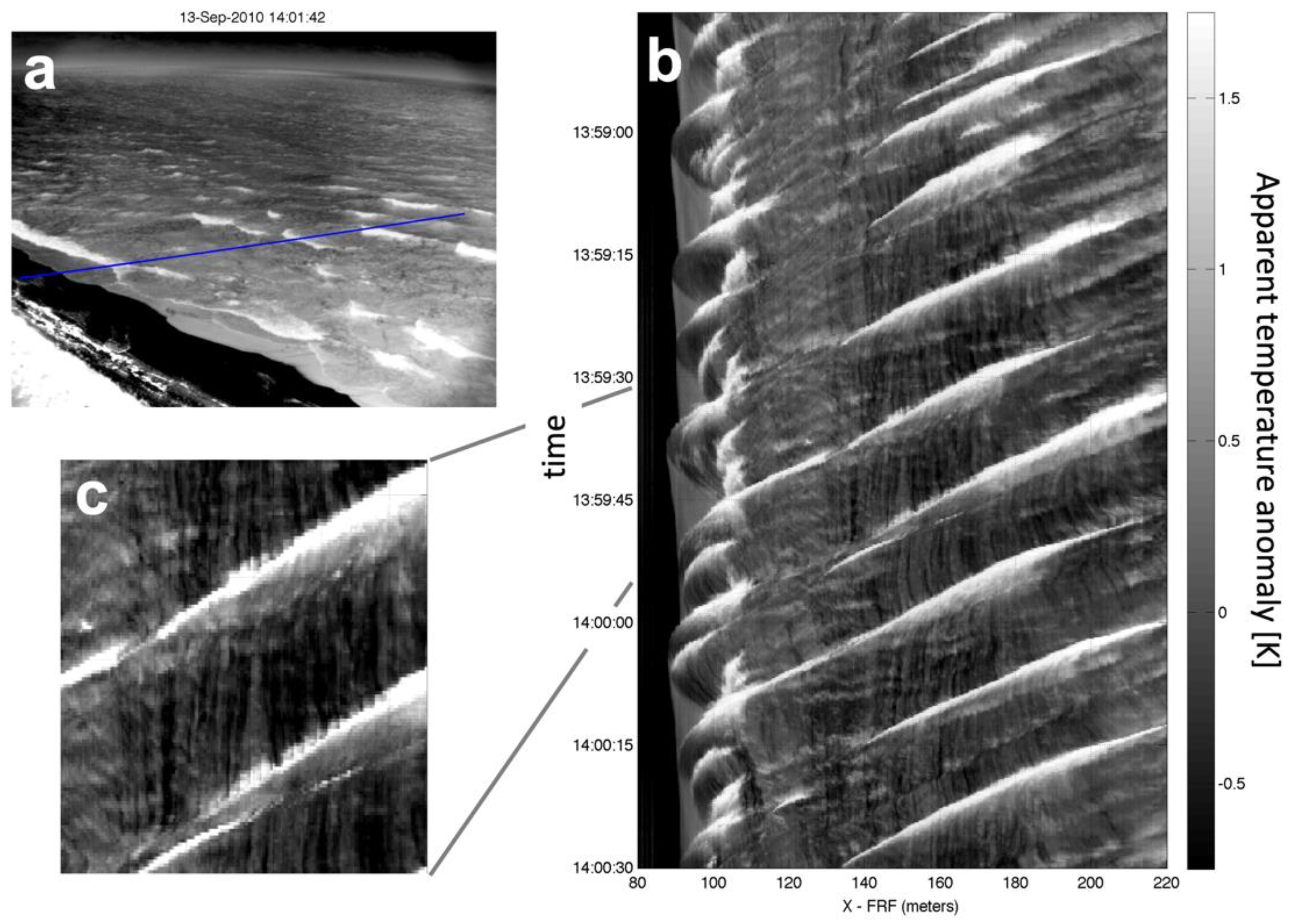
Cooler residual foam is a ubiquitous signature of breaking waves. Figure 1a shows an IR image of breaking waves acquired in the early morning (0900 EDT, 1400 UTC, 13 September 2010) from a tower-mounted IR camera viewing shoaling and breaking waves at the beach of the USACE Field Research Facility in Duck NC [29]. A Hovmöller (time and space) diagram of cross-shore IR brightness temperature taken from Figure 1a is shown in Figure 1b, and Figure 1c is an expanded section of Figure 1b. The oblique traces of the bright (warm) surface show the actively breaking faces of waves, while the darker (cooler) and more long-lived foam patches in the wakes of the breaking waves appear as the vertical streaks. In this example, the stable foam cools within seconds of the passage of an active wave front by 0.5 °K to 1 °K compared to the nearby non-foam covered water surface.

Cooling of residual foam has relevance for thermal remote sensing of the ocean surface. Based on the observations of [27], cooling foam whitecapping could cause an error in surface temperature estimates from satellites if the magnitude of the cooling is the same as that of the cool skin correction [30,31]. Furthermore, [29] showed that the difference in the IR brightness temperature between cooling foam and actively breaking wave crests can be used to isolate the dynamic portion of the wave. The active portion of the breaking wave, also called the roller or stage ‘A’ breaking wave [32], was identified by [29] using IR wavelengths, which had a distinct advantage over using imaging in visible wavelengths where the actively breaking crests and foam have nearly an equally bright signature. Finally, thermal IR imagery of cooling seafoam and warmer breaking wave crests was also shown to correlate with microwave brightness temperatures of the passive and active stages of wave breaking [33].

The mechanism for rapidly cooling residual foam is not definitively known, though [27] argue that evaporative cooling plays a central role. Their hypothesis is that, once formed, the water-to-air sensible and latent heat fluxes from the thin surface film of water in the residual foam will be much larger than the heat fluxes through the undisturbed water surface. Moreover, the small volume of water contained in the thin bubble walls at the air–water interface (O (2–10) μm thick, e.g., [34]) and restricted exchange of the interstitial water with the bulk water phase below the foam imply the temperature decrease of the foam due to the cooling could be amplified by the relatively small thermal mass of the foam compared to the underlying bulk water.

The importance of bubbles and spray drops from foam bubbles bursting to the heat flux through seafoam is not clear. The latent and sensible heat flux of bubbles from wave breaking were estimated by [5] using standard gas and heat flux formulae and available bubble size distributions. They estimated that the bubble-mediated heat flux at winds speeds greater than 25 m s⁻¹ is less than five percent of the net heat flux. Near surface temperature data were analyzed by [4] and suggested that bubbles are not a significant factor in cooling the ocean surface. Spray can directly contribute to the water heat flux when the droplets exchange heat with the atmosphere and reenter the water, communicating the heat loss or gain back to the water body [35]. Measurements of enthalpy (total heat) transfer made by [36] in a laboratory wind tunnel showed a decrease in the enthalpy transfer coefficient for wind speeds from 0 to 4 m/s followed by an increase at higher wind speed when spray was present. Spray can indirectly modulate the air–water heat flux through altered evaporation and humidity profiles.

In this work, we measure heat loss from foam-free and foam-covered seawater surfaces, with the foam being generated by a subsurface diffuser. The results are relevant to stage B [32] residual foam in the wake of a breaking wave rather than to the Type A actively generated foam. Using a laboratory wind tunnel, we carefully controlled the bulk air–water temperature difference, relative humidity, and wind speed conditions provided. Latent and sensible heat fluxes between the water and the air are calculated with a control volume technique. We will not directly examine the role of spray but examine the assumption that the observed cooling of foam on a seawater surface is due to the enhancement of heat fluxes from sea foam compared to a foam-free seawater surface. To the best of our knowledge, these are the first direct measurements of the heat flux due to sea foam.

2. Materials and Methods

2.1. Heat Flux Estimation

Air–water heat flux estimates were made based on air-side measurements of vertical profiles of temperature and humidity upwind and downwind of a foam-covered water surface. As shown below, this method allows for explicit separation of the heat transfer components from the total heat flux.

The wind tunnel is considered to be a control volume, thus heat loss from the water surface can be estimated through the net balance between the upwind and downwind sensible heat content and water vapor (i.e., latent heat),

$$Q_T=Q_s+Q_L+Q_R$$

(1)

where Q represents heat flux (J s⁻¹) and the subscripts are defined as follows: T represent the total net flux, S represents the sensible component, L represents the latent component, and R represents the radiative component, respectively. The heat flux components were computed from:

$$Q_L=\frac{L_w{\rho }_a}{A_s}{\displaystyle \underset{A}{\iint }\left(q_d-q_u\right)U_{d}dA}$$

(2)

$$\begin{array}{c}{Q}_s=\frac{c_{pa}{\rho }_a}{A_s}\left({\displaystyle \underset{A}{\iint }\left(1-q_d\right)T_d{U}_{d}dA-{\displaystyle \underset{A}{\iint }\left(1-q_u\right)T_u{U}_{u}dA}}\right)+\\ \frac{c_{pw}{\rho }_a}{A_s}\left({\displaystyle \underset{A}{\iint }{q}_d{T}_d{U}_{d}dA-{\displaystyle \underset{A}{\iint }{q}_u{T}_u{U}_{u}dA}}\right)\end{array}$$

(3)

$$Q_R=\sigma \left(T_{skin}^4-T_u^4\right)$$

(4)

where L_w is the latent heat of vaporization, c_pa is the heat capacity of dry air, ρ_a is the air density, T is measured air temperature, U is the wind velocity, q is water vapor mass fraction, and A is the cross-sectional area of the air flow, and σ = 5.67 × 10⁸ is the Stefan–Boltzmann constant. A is taken as the cross-sectional area of the air outflow over the tank surface, which is affected by the surface heat flux, and A_s is the surface area of the tank (0.258 m²). Measurements upwind and downwind of the foam or water surface are denoted by u and d subscripts, respectively, and q and ρ_a were determined through standard relationships using the measured atmospheric pressure, air temperature, and relative humidity. Net radiative heat flux is calculated as the difference in the total radiation, estimated via the Stefan–Boltzmann law, of the surrounding wind tunnel walls (assumed to ambient temperature) and the water surface skin temperature, similar to [23]. Finally, Equation (1) describes the enthalpy change of the air in the system, Q_E, if the net radiative heat flux is neglected. In these measurements, Q_R is small because the wind tunnel and water temperature are approximately equal, thus we will be using Q_E in place of Q_T going forward.

2.2. Laboratory Measurements

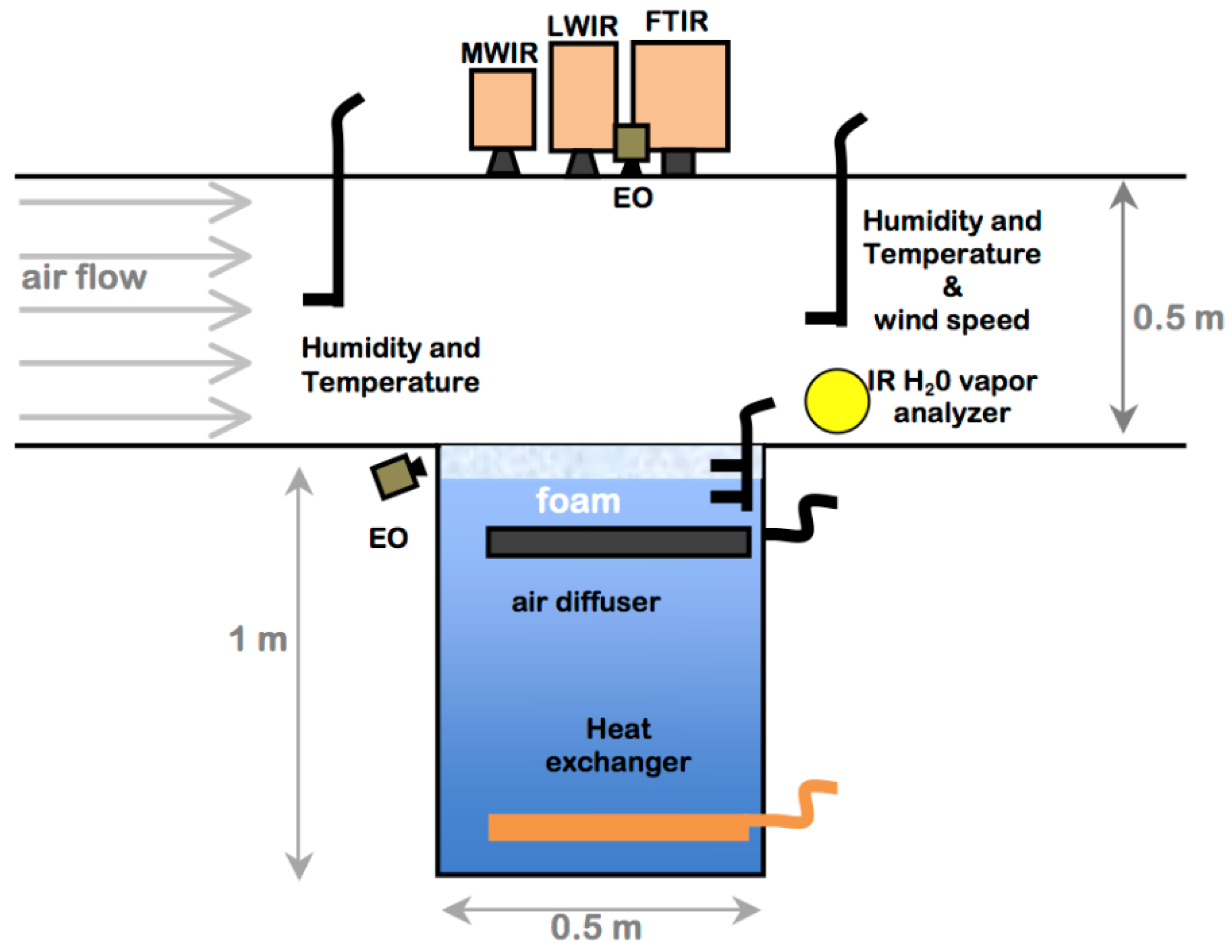
Laboratory experiments were performed in the wind-wave tunnel described by [37]. The system is comprised of a test tank 0.5 m × 0.5 m in cross section and 1 m deep imbedded in the center of a wind tunnel. The wind tunnel has a test chamber 0.5 m × 0.5 m in cross-section and 1.5 m in length as shown in the schematic in Figure 2. The modest dimensions of the facility allow both detailed air and water measurements and careful regulation of the air flow and water conditions. The wind turbine is tuned to provide stable low speed airflow (0–5 m/s). Airflow through the test section is drawn from the room housing the wind tunnel with temperature and humidity controlled by an industrial HVAC system. Low humidity conditions were achieved by running the HVAC system, while leaving the HVAC system off for one to two days with the tank lid open would gradually increase the relative humidity in the room air.

Natural, filtered seawater was used in the tank for all tests, and sodium hypochlorite was periodically used to control bacterial growth and contamination. Prior to the start of measurements on a given day, the water surface was cleaned of dust and surfactants through suctioning and physical wiping of the surface with lint-free optical paper [38]. A layer of saltwater foam approximately 1.7 cm thick was generated by forcing compressed laboratory air at a rate of 0.4 l s⁻¹ that had been filtered to remove water and oil through a submerged diffuser in the tank. The diffuser, positioned 10 cm below the mean water level, was made from gas-permeable tubing, similar to that used in previous laboratory experiments [39,40] and field simulations of seafoam [8]. Bubbles entrained in salt water will equilibrate with respect to temperature and water vapor concentration within one second of formation [5]. The mean diameter of bubbles produced by the diffuser was estimated to be 1 mm, and bubbles of this size have a terminal rise velocity of 10 cm/s. This implies a residence time of 1 s in the water layer below the foam. Bubbles in the foam layer will travel vertically at roughly the ratio of the void fraction volume (approximated as the foam volume times 0.74, a sphere close packing filling efficiency) to the air flow rate, which gives an approximately 8 s residence in the foam layer. Thus, bubbles would have adequate time to equilibrate before reaching the air–water interface.

Temperature in the bulk tank water was regulated to within 0.5 °C using a flow-through, constant temperature heat exchanger, and before each experimental test the heat exchanger was turned off. Heat loss to the room through the tank walls was minimized by 6 cm thick rigid polyisocyanurate foam insulation fixed to the four vertical sides of the tank, and the bottom of the tank was left exposed.

A thermal infrared camera viewed and recorded the scene through a 5 cm diameter port in the top of the test section. The IR camera was a long-wave infrared, QWIP array imager (FL 640 QLW, AEG INFRAROT-MODULE GmbH) measuring in the 8 to 10 μm wavelength band with a 640 by 480 pixel array. The thermal camera was positioned to view the foam surface at a distance of 50 cm from an off-nadir angle of 10° to avoid direct camera reflection giving a spatial resolution of 0.05 cm per pixel. IR imagery was captured at a frame rate of 20 Hz. The top of the wind tunnel test section was constructed of a 6 mm thick aluminum plate coated with a high-IR emissivity paint and insulated on the top side with 6 cm thick polyisocyanurate foam. The insulated tank ceiling minimized both temperature gradients in the air phase not caused by air–water heat exchange and reflections of the tank in the IR images. The IR camera was corrected for nonuniformity and calibrated to radiometric brightness temperature using a precision blackbody target (Santa Barbara Infrared model 11104) with an assumed emissivity of unity. A two-point calibration scheme was used, with reference calibration temperature images acquired with the black body temperature set 1 °C above and below the initial bulk water temperature.

In-water tank measurements consisted of a vertical array of six calibrated thermistors (Sable Systems TC-2000, type T) spaced at 0.2, 0.6, 1.0, 1.8, 5.2 and 7.2 cm depth from the air–water/foam interface with the top four thermistors positioned to nominally sample in the foam layer. The thermocouples were calibrated prior to the experiment in a NIST traceable constant temperature bath to reduce the maximum absolute temperature error to 0.05 °C. Air-side instruments were mounted at a constant height of 2.5 cm above the mean water level. These sensors were: thermistors mounted upwind and downwind of the water tank; an open path Li-Cor LI-7500A water vapor analyzer (WVA) mounted downwind of the test section; and a cup and vane anemometer mounted downwind of the WVA. Heat flux time series were measured over a range of wind speeds, from 0.5 m s⁻¹ to a maximum wind speed of 2.5 m s⁻¹ to prevent foam and spray from leaving the test section and contaminating the downwind water vapor and temperature measurements. Test conditions spanned air–water temperature differences of −9 °C to 0 °C (a negative value indicates air cooler than water), and ambient relative humidity from 40% to 78%.

3. Results

3.1. Heat Flux

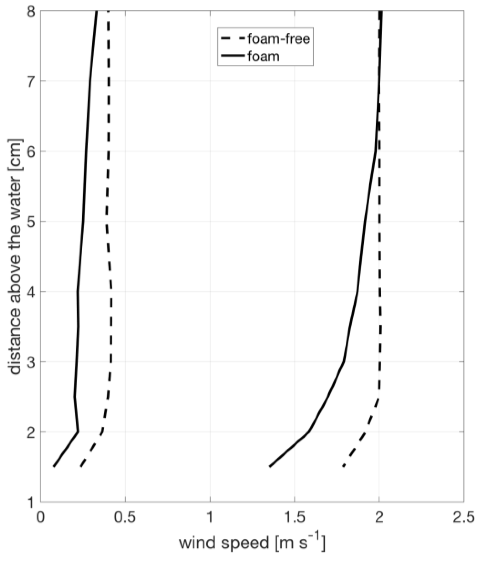
Velocity profiles measured using the traversing pitot tube, shown in Figure 3, demonstrate that the boundary layer over the water surface has a height of approximately 6 cm over foam and 3 cm over foam-free surface, which is expected given the increased roughness of the foam layer. Therefore, our measurement of temperature and humidity at a fixed height of 3 cm just downstream of the tank is within in that boundary layer. We use a fixed 3 cm layer depth for all calculations as a standardization to allow for consistent comparison between foam and foam-free conditions. Implications of this methodology are examined in the discussion.

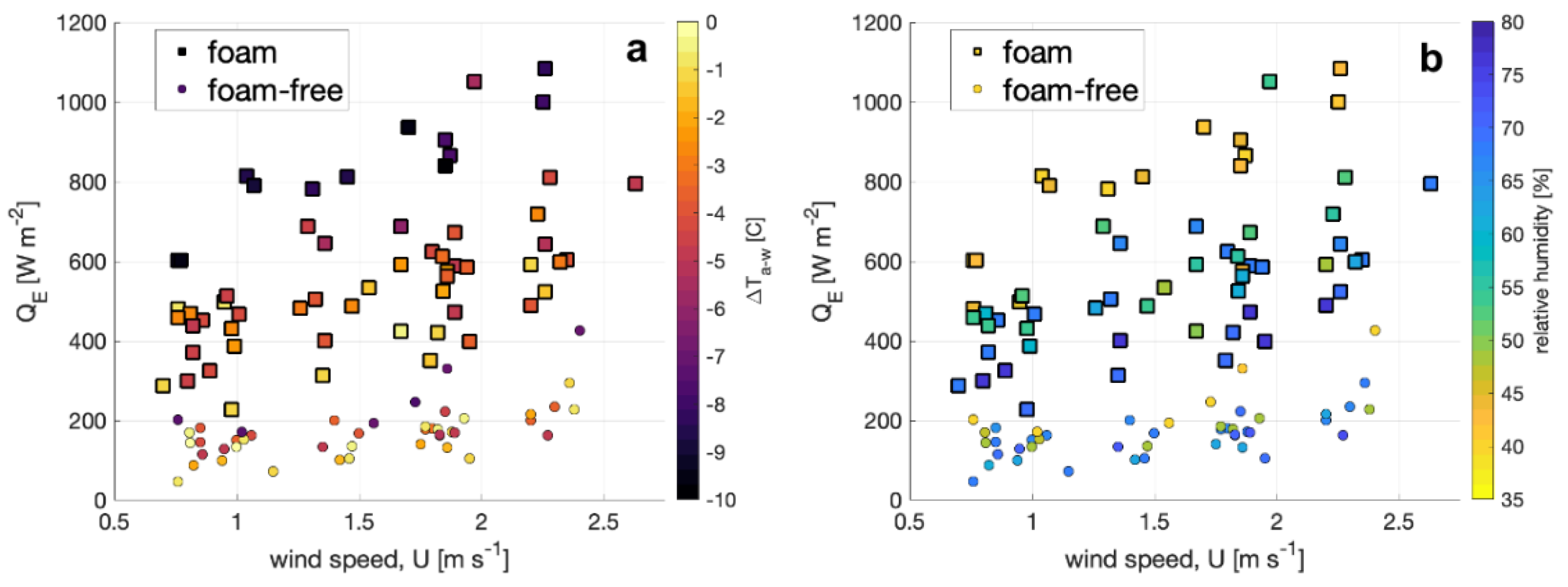
The enthalpy flux Q_E is shown for foam-covered and foam-free water surface in Figure 4 plotted as a function of wind speed and segregated by air-water temperature difference (Figure 4a) and relative humidity (Figure 4b). The enthalpy flux is a factor of three to four larger at a given wind speed, air–water temperature difference (ΔT_a-w), and relative humidity (RH) for a foam-covered surface compared to Q_E for a foam-free surface. At a given wind speed, Q_E for the foam-covered cases is also correlated with RH and ΔT_a-w. Unsurprisingly, the highest values for Q_E occur for the lowest RH and most negative ΔT_a-w (air cooler than water), conditions that favor the largest upwards latent and sensible heat fluxes, respectively. The correlation of Q_E with RH and ΔT_a-w is also observed for foam-free surfaces, although it is most notable for the most negative ΔT_a-w and smallest RH.

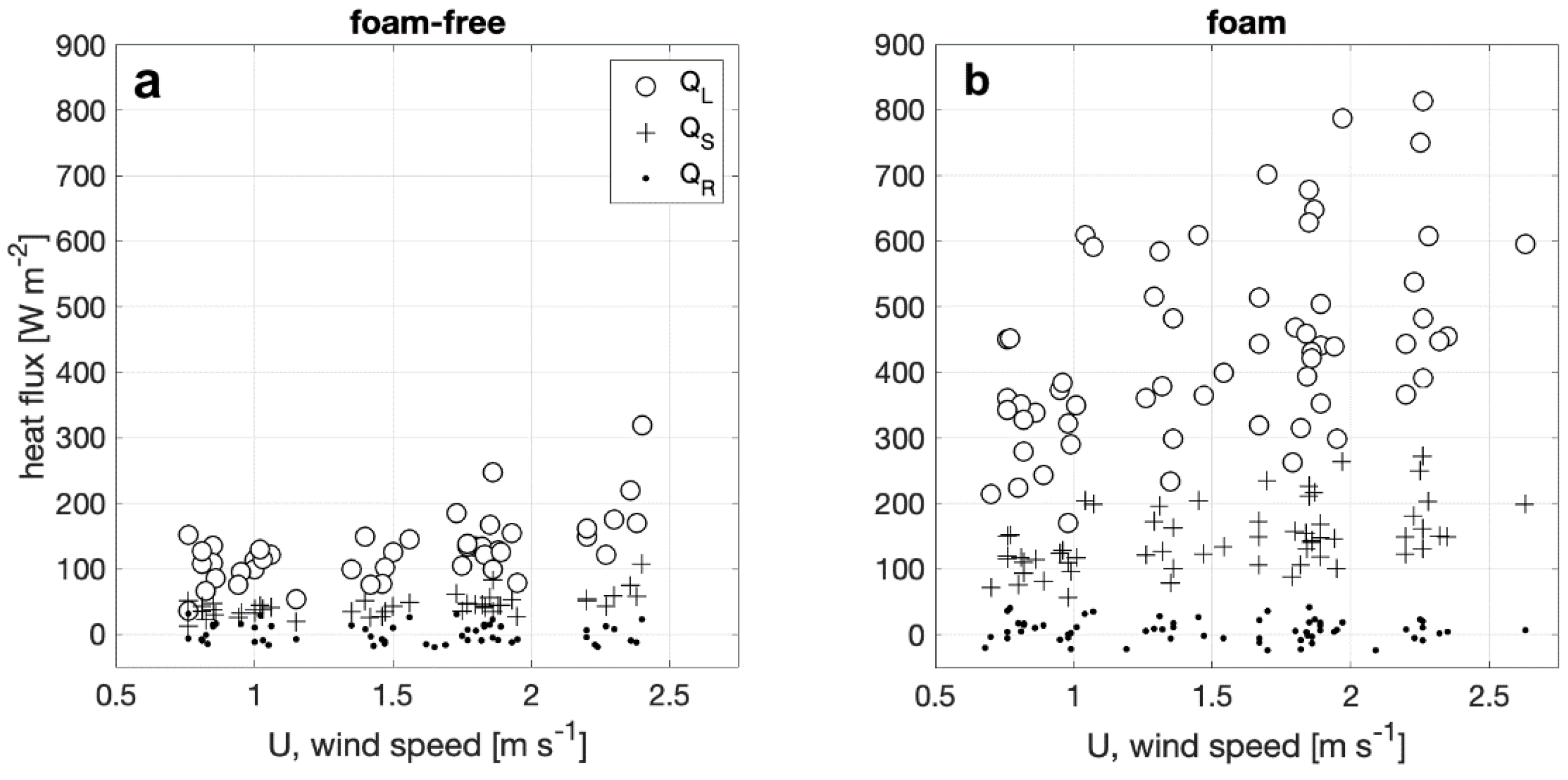
Net heat flux components Q_S, Q_L, and Q_R from foam-covered and foam-free surfaces are plotted against wind speed in Figure 5. Overall trends indicate both Q_S and Q_L increase with increasing wind speed. Q_L dominates Q_E under the conditions tested for both foam-covered and foam-free surfaces. This result for foam-free conditions is consistent with previous measurements [36]. Furthermore, Q_L and Q_S from the foam-covered surfaces increase up to two and three-fold from a foam-free water surface. The magnitude of the net radiative heat flux, Q_R, is on average 12 and 18 W m⁻² for foam-free and foam surfaces, or 7% and 3% of Q_E, respectively. As Q_R only depends on differences between water and wind tunnel wall temperatures, variation with wind speed and relative humidity is not observed.

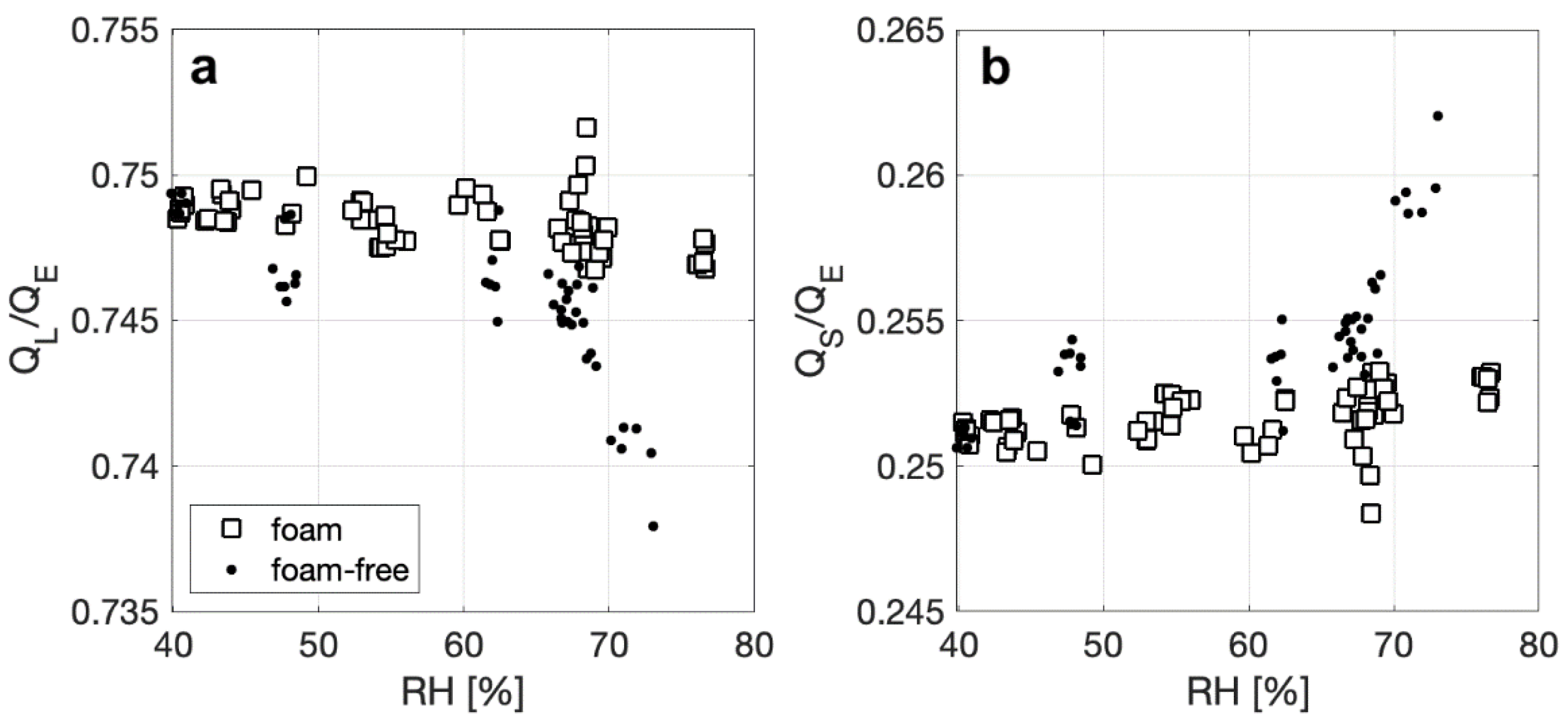
We further explore the enhancement of in latent heat flux for foam by calculating the ratio of Q_L to Q_E and the ratio of Q_S to Q_E. Overall, foam and foam-free surfaces have an approximate and consistent split of 75% of Q_E due to latent heat transfer, and 25% due to sensible heat transfer, with no discernable dependencies on ΔT_a-w, though observable trends do exist compared with RH. The plot of Q_L/Q_E versus RH in Figure 6a shows that, for both surfaces, the fraction of Q_E that is due to the latent heat flux decreases slightly as RH increases, with the change of Q_L/Q_E in RH being more apparent for a foam-free surface (0.75 to 0.74). This decrease in relative importance of Q_L as RH increases could be a result of a decrease in the water–air specific humidity gradient that drives the latent heat flux. Figure 6b shows the complimentary effect, where Q_S/Q_E shows a slight increase as RH increases, but to a larger degree for a foam free-surface (0.25 to 0.26) as RH increases. Overall, this suggests that small changes in the latent heat flux for a foam surface will have a greater effect on the total net heat flux for a range of RH conditions.

3.2. Vertical Water Temperature Profiles and Water-Surface Skin Temperature

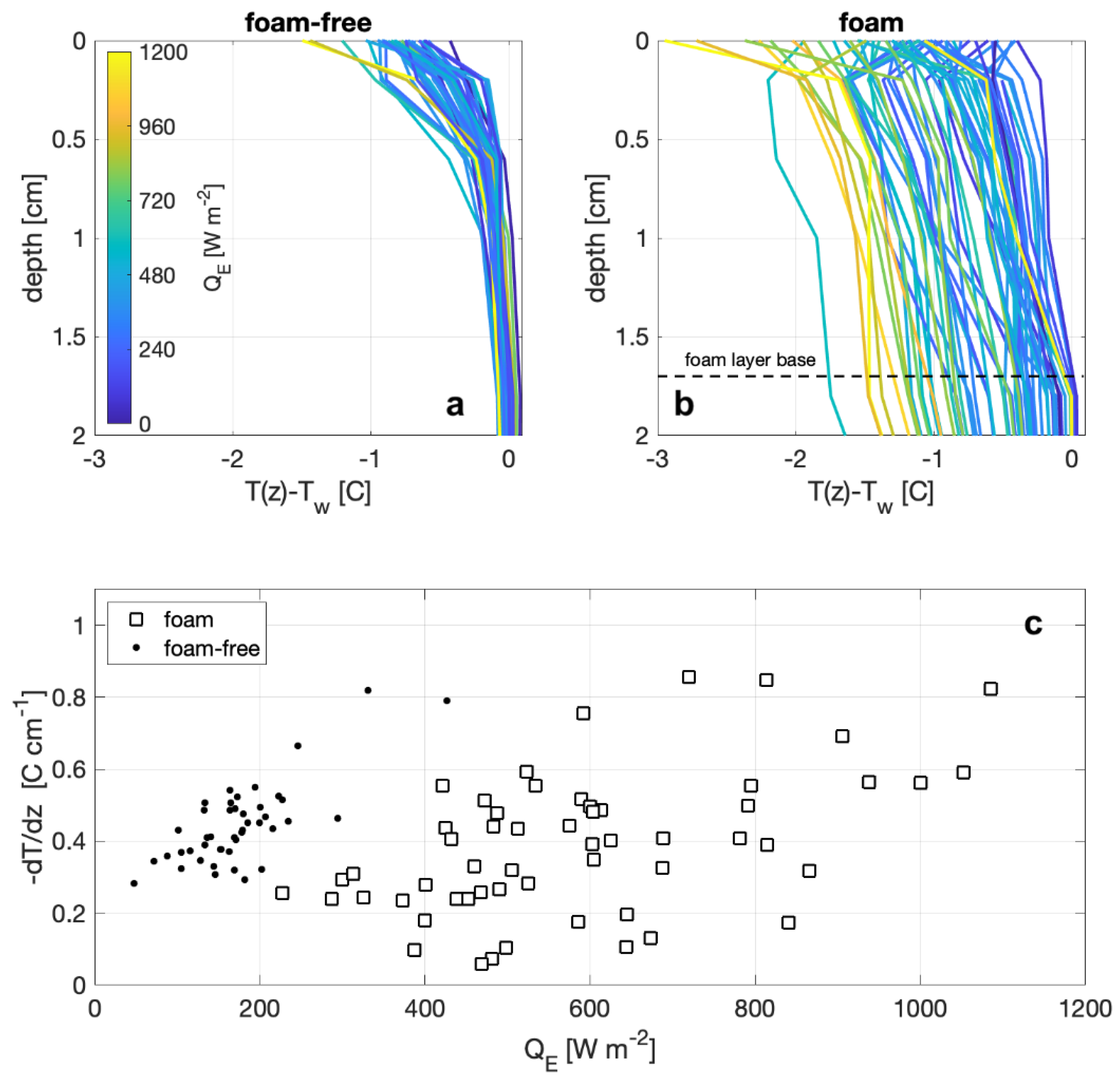
Measurements from the vertical temperature array show distinct differences between observations with and without foam on the surface, as shown in Figure 7. The profiles are plotted as the difference of the temperature at the measurement depth and the temperature at a depth of 7.2 cm (i.e., the deepest measurement depth), where depth is defined as the distance to the air–foam or air–water interface, and the surface temperature (depth = 0) is the radiometric temperature. The temperature profile for a foam-covered surface (Figure 7b) are approximately linear near the surface and show that the surface temperature differs from the bulk temperature, below the foam layer, with the largest differences corresponding to larger measured Q_E. Temperature profiles in the absence of foam (Figure 7a) show exponential increases in the surface temperature that closely resemble those investigated by [41]. However, the overall temperature differences of the non-foam profiles do not seem to be correlated with observed heat fluxes, but instead the near-surface temperature gradients, from 0 cm to 1.8 cm (Figure 7c), are negatively correlated with observed Q_E. The near-surface temperature gradients within foam show little to no correlation with measured heat flux. Thus, the general difference between the shape of the profiles is consistent with the enhanced mechanical mixing due to the foam generation. In the absence of foam, convective mixing from surface cooling and forced overturns from wind stress become the largest influences.

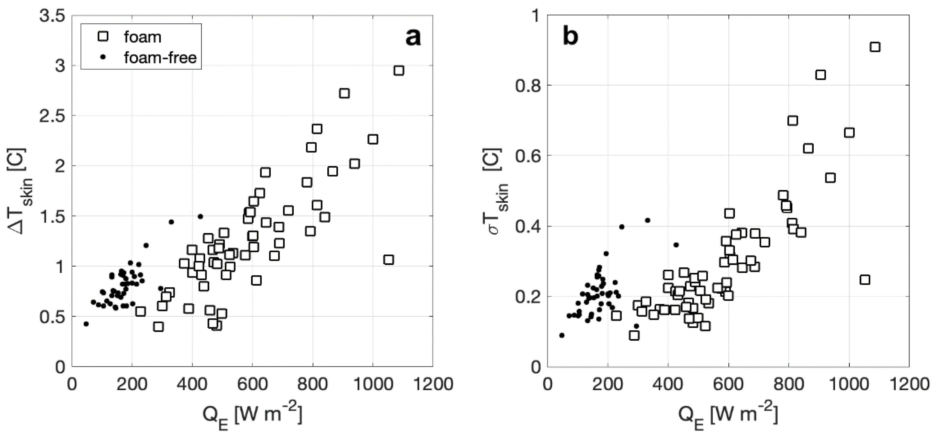
Here, we define the bulk-skin temperature difference, ΔT_skin, as the temperature measured at 7.2 cm depth minus the radiometric brightness temperature from the calibrated IR camera, T_IR, with ΔT_skin positive indicating a cooler skin temperature. The skin temperature variability, σT_skin, is calculated as the standard deviation of the temperature distribution in the image over the measurement period. Plotted in Figure 8a, ΔT_skin for both surface types varies approximately as a linear function of Q_E with the magnitude of ΔT_skin increasing with increasing heat flux, consistent with the expected relationship proposed by [42]. The range of ΔT_skin with foam is twice as large as ΔT_skin without foam and the heat flux range with foam is several times large than without foam. In Figure 8b, σT_skin is shown to have patterns similar to ΔT_skin, where the overall skin temperature distribution increases with increasing heat flux, and σT_skin has a larger range for a foam surface. For foam-free surfaces, σT_skin increase more rapidly and is larger than a foamy surface for similar Q_E.

4. Discussion

4.1. Bulk Heat Flux Parameterization

The observed enthalpy flux is parameterized based on wind speed and a linear enthalpy gradient assumed from standard observations,

$$Q_T=\rho C_{k}U\left(k_s-k\right)$$

(5)

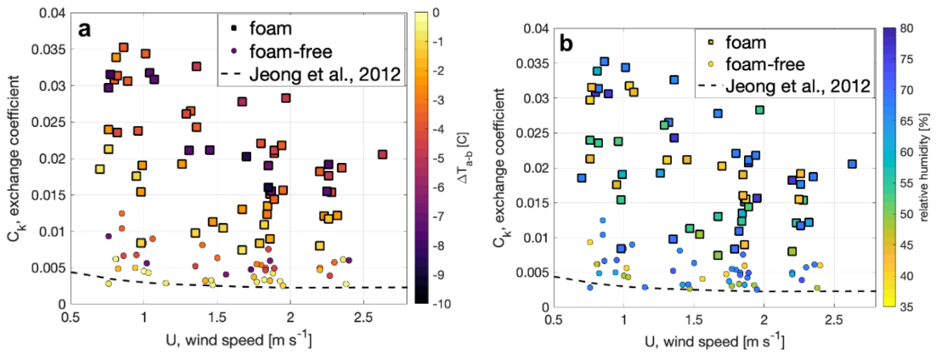
where C_k is the enthalpy exchange coefficient that can be determined from our observations, k is the enthalpy observed at a standard height and k_s is the surface enthalpy calculated for saturated air. The enthalpy for saturated air under the observed conditions was computed following conventional meteorological parameterizations. The resulting determination of C_k is shown in Figure 9 and demonstrates the expected decrease of C_k under light winds over both surfaces, and the new result that the enthalpy exchange from the foam surface is up to a factor of four larger than foam-free surface. The results also show that C_k is a function of the air–water temperature difference (Figure 9a), where C_k is larger, for a given wind speed, when the water temperature is warmer than the air. In contrast, C_k does not appear to depend on relative humidity (Figure 9b).

Our enthalpy exchange coefficients for foam-free conditions are compared with values for foam-free conditions reported by [36] in Figure 9. The comparison shows a similar trend of decreasing C_k with increasing wind speed and that the measurements by [36] agree with our measurements at small air-bulk temperature difference. Further quantitative comparisons with [36] are precluded by differences in experimental conditions such as fetch and location of the air temperature measurements above the surface.

4.2. Spray and Bubble Effects

Spray and its contribution to the observed net heat flux was not explicitly measured during this experiment. However, many of the spray jet and film drops (diameters 10–100 μm) produced from bubble bursting would have had the opportunity to reenter the tank and not blow outside the test area, except at the highest wind speeds, as we noted only minimal water accumulation immediately downwind of the test section. As we did not measure the spray production, we cannot assign the fraction of the heat flux due to the presence of spray, though [36] estimated that spray mediated component of C_k could be as much at 38% for conditions with wind generated waves and spray in a flume.

There is an additional heat flux arising from the foam generation due to heat flux to the bubbles during their creation. In our experiments, we inject compressed ambient-temperature air into the diffuser. As the compressed air is allowed to cool to room temperature before it enters the diffuser, upon decompression in the diffuser, it cools due to adiabatic expansion. However, there is also a cooling term, as water vapor evaporates into the bubble after it forms. In the following calculations, we assume conditions for maximum enthalpy flux from the water so that the air bubbles rising from 10 cm depth will both completely equilibrate in terms of temperature and water vapor before they rise to the surface with the net effect of cooling the water in the tank. Thermal and water vapor equilibrium of the bubbles during their rise time is reasonable. The millimeter diameter bubbles generated here have rise velocities in the order of 0.1 m s⁻¹ [43,44] and subsequent rise times in the order of 1 s to the foam layer. Calculations by [4] indicate these bubbles will thermally equilibrate in less than 0.3 s. Following the methodology of [4], the bubble equilibration time scale for water vapor was estimated by [5] to be an order of magnitude shorter than the thermal equilibrium time scale. The net heat flux from the water to atmosphere via bubble formation, Q_b, is

$$Q_b=F_a\left[{\rho }_a{c}_{pa}\left(T_w-T_d\right)+L_w{q}_s\right]$$

(6)

where F_a is the volumetric air flux through the diffuser, T_d is the diffuser air temperature (measured at 2.7 K cooler than ambient temperature due to adiabatic decompression), and q_s is the specific humidity at saturation. Equation (6) assumes that the air entering the bubble diffuser is completely dry, and that the latent heat is transferred to the bubbles from the water. The resulting Q_b from the observed conditions during foam production range from 67 to 120 W m⁻² with an average of 93 W m⁻². The portion of Q_b due to the bubble-mediated latent heat flux ranges from a low of approximately 80% (i.e., a latent flux of 95 W m⁻² when Q_b is 120 W m⁻²) to a high of approximately 95% (i.e., a latent flux of 64 W m⁻² when Q_b is 67 W m⁻²). Compared to the values for the component heat fluxes shown in Figure 5a for a foam-free surface, Q_b represents a doubling of the net water-to-air heat flux. As discussed below, because Q_b is a major component of the net heat flux through a foam-covered surface, we hypothesize that the bubble-mediated heat flux plays a central role In creating the cool foam.

These calculated bubble-mediated heat fluxes explain the increases in component heat fluxes between foam-free and foam-covered surface seen in Figure 5a,b, respectively. Furthermore, this additional source of sensible and latent heat to the air phase from the bubbles works to create an unstable boundary layer, as shown in the wind speed profiles in Figure 3. The unstable boundary layer increases upward mixing and increases the latent and sensible heat transfer not due to bubbles.

4.3. Vertical and Horizontal Surface Thermal Structure

The foam-free temperature profiles (Figure 7) show the characteristic exponential decay of temperature with depth of a logarithmic boundary layer profile. This boundary layer in the water is unsurprising given the relatively low wind speeds in the tunnel. However, at similar values of Q_E, the temperature profiles in the foam-covered cases start at a lower temperature and do not increase as quickly with increasing depth as the temperature profiles for the foam-free cases. As a result, water temperature at a particular depth is lower when foam is present than under a foam-free surface (for the same Q_E). This shows the cool-foam effect is not just a surface effect (i.e., a lower skin temperature), but reflects cooling that extends through the foam and into the bulk water beneath. Furthermore, the smaller temperature gradients at similar Q_E between foam and foam-free shown in Figure 7c indicate that the transfer velocity for the vertical transport of heat is larger for a foam-covered surface than the transfer velocity for the foam-free case. Figure 3 shows that the presence of foam causes the air-side boundary layer to deepen. Figure 5 shows that at a given wind speed, the latent and sensible heat fluxes through a foam-covered surface are nearly double those at foam-free surfaces.

These three observations concerning the differences between a foam-covered and foam-free surface lead us to propose that the cool foam effect is due to the foam both decreasing the thermal mass of the surface in contact with the air and increasing the net water-to-air heat flux. The effect of the decrease in thermal mass is seen by considering the void fraction of the foam. Given the foam thickness (1.7 cm), the volumetric flow rate of air (400 cm³/s), and the surface area of the tank (2500 cm²), we estimate that the foam void fraction is between 0.80 and 0.94 with a mean bubble residence time on order of 10 s. Note that this is much higher than the densest regular packing of a collection of spheres, because as the foam ages and the interstitial water drains, the bubbles deform from spherical shape with an increase in void fraction [45]. If the presence of the foam does not affect either the transfer of heat through the water or the water-to-air heat flux, the temperature decrease for the foam would be ten times that of a foam-free surface, since the heat loss is coming from a smaller mass of water.

Figure 7b shows the measured cooling in the foam is in the order of 3 °C, whereas we predicted a cooling of 10 °C based on the estimated void fraction and resulting change in thermal mass of the foam layer. The smaller foam cooling suggests that the foam increases transport of heat upwards through the water column. Furthermore, the relatively small temperature gradient through the foam layer (Figure 7c) is suggestive of the increased mixing in the foam compared with the exponential temperature gradients in the foam-free profile. This reveals the process differences that occur between a foam-covered and foam-free surface are due to rising bubbles in the foam layer. Our conceptual model for the near-surface temperature profile with active foam generation is that the more homogenous layer results from enhanced mixing. Warmer bulk water is continually brought to the base of the foam layer by continual bubble supply from the foam generator. Within the foam layer, bubbles from below replace bubbles at the surface as they thin and burst, thus moving water to the surface. As the bubble and surrounding water move through the foam layer, the air in the bubble warms due to the sensible heat flux into the bubble while the surrounding fluid cools due to the latent and sensible heat fluxes into the bubble. The combination of the net upward heat flux through the surface combined with the cooling of the water surrounding the bubbles both form the cool foam and is responsible for the increase in the net heat flux.

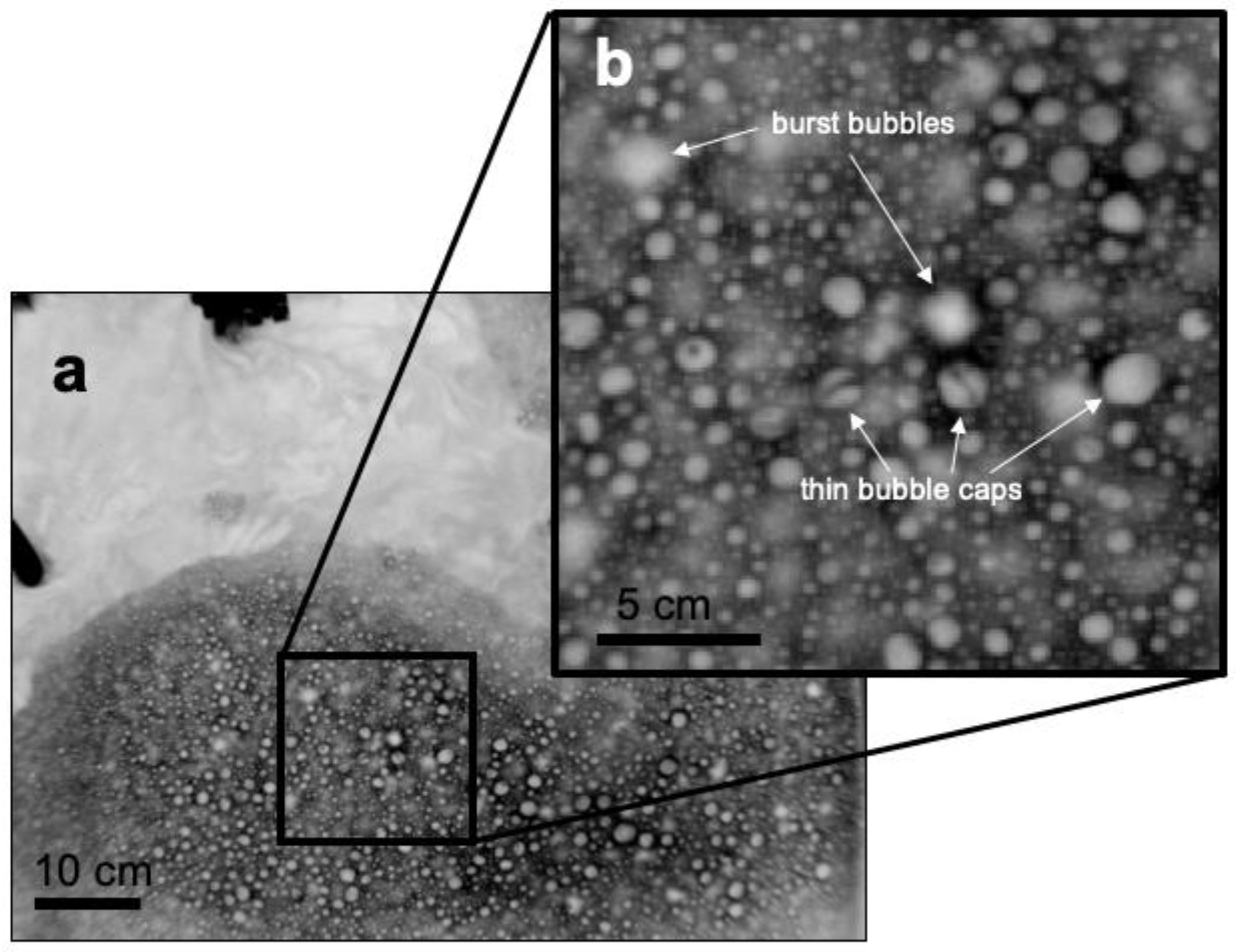
Figure 8a shows that at a particular value of Q_E, ΔT_skin for a foam-covered surface is approximately a factor of two smaller than ΔT_skin for a foam-free surface. This result is consistent with our proposed mechanism since when foam is present, approximately half of the total water-to-air heat flux is supported by the bubble-mediated sensible and latent heat fluxes. The measured bulk-skin temperature difference represents the free energy gradient driving the non-bubble related heat fluxes, and as discussed above, the presence of the foam does not affect these significantly. The decrease in σT_skin between foam-covered and foam-free surfaces is also consistent with our model since the decreased thermal mass of the foam layer would work to homogenize horizontal temperature gradients. For reference to this explanation, Figure 10 shows a detailed image of the mottled appearance of foam from a time seconds after the foam generator has been shut off, where bubbles exist as both warm and cool over the surface of the foam layer. As seen in Figure 10, this affect is analogous to the cool stage B, or residual foam, observed by [27].

This conceptual model also has implications for thermal remote sensing applications of breaking waves. Cooled, residual foam was observed in the field by [27] and the cool foam was used by [29,46] to isolate the active part of a breaking wave from the passive residual foam. In an oceanic whitecap, bubbles form from the collapsing large void cavity of surface air entrained in the breaking wave [46]. For ocean conditions of a net heat flux from the ocean to the atmosphere driven by both an upwards latent and sensible heat flux, this would give a bubble population with a gas phase that is cooler than the surrounding water and under-saturated with respect to the water vapor concentration. Although the specific humidity and temperature gradients in these whitecap bubbles might not be as large as the laboratory bubbles used here, the direction of the heat fluxes would be the same, so it is reasonable to assume the cool-foam effect seen in oceanic breaking waves results from a mechanism similar to that proposed here. However, we were not able to examine the transition from the warmer actively breaking wave to the development of the cool residual foam as was seen in [27].

5. Conclusions

Combining data from laboratory experiments with a control volume approach, we calculate net heat fluxes from foam on seawater to air over a wind speed range of 0.5 to 2.5 m s⁻¹, an air–water temperature difference range of −9 to 0 °C, with relative humidity from 40% to 78%. Results show that, for the same wind speed, air–water temperature difference, and relative humidity, a foam-covered surface can enhance the net air–water heat flux by up to a factor of four relative to a foam-free surface. We hypothesize that this increase in net heat flux is due to a sensible and latent heat flux to the bubbles as they are submerged in the water. As the bubbles burst at the surface, this heat is transferred to the air phase, bypassing transfer through the air–water surface. The additional heat flux from the bubbles combined with the lower thermal mass of the foam layer leads to the formation of the cool-foam effect. The bubble-mediated heat flux also creates an unstable boundary layer in the air over the water.

The heat flux from foam increases with increasing wind speed, decreasing air–water temperature difference (air cooler than water), and decreasing ambient relative humidity. The effect of air–water temperature difference seems to have a more direct correlation to higher heat fluxes for a given wind speed than ambient relative humidity. Enthalpy exchange coefficients computed from the observed heat fluxes for foam decrease with increasing wind speed and are two to four times the exchange for foam-free conditions, which agree with the foam-free conditions measured earlier by [36] in a wind-wave flume. We speculate that the convergence of enthalpy exchange coefficients between foam and foam-free conditions, observed for our low wind speeds, may likely converge further under high wind speeds, at which point foam and spray are generated naturally by whitecapping. These results reinforce the cool, residual seafoam observations of [27] and provide a mechanism for the phenomenon. Overall, we found enhanced cooling in the radiometric skin temperature of foam relative to a foam-free surface. Further analysis showed a decrease in skin temperature variability for foam, which was due to directly to the presence of bubbles at the surface, and we developed a conceptual model to explain this in terms of the thermal mass of the foam layer.

References

- Wallace, D.W.R.; Wirick, C.D. Large air-sea gas fluxes associated with breaking waves. Nature 1992, 356, 694–696. [Google Scholar] [CrossRef]
- Farmer, D.M.; McNeil, C.L.; Johnson, B.D. Evidence for the importance of bubbles in increasing air-sea gas flux. Nature 1993, 361, 620–623. [Google Scholar] [CrossRef]
- Melville, W.K. The role of surface-wave breaking in air-sea interaction. Annu. Rev. Fluid Mech. 1996, 28, 279–321. [Google Scholar] [CrossRef]
- Farmer, D.M.; Gemmrich, J.R. Measurements of temperature fluctuations in breaking surface waves. J. Phys. Oceanogr. 1996, 26, 816–825. [Google Scholar] [CrossRef] [Green Version]
- Andreas, E.L.; Monahan, E.C. The role of whitecap bubbles in air-sea heat and moisture exchange. J. Phys. Oceanogr. 2000, 30, 433–442. [Google Scholar] [CrossRef]
- Andreas, E.L. Sea spray and the turbulent air-sea heat fluxes. J. Geophys. Res. Oceans 1992, 97, 11429–11441. [Google Scholar] [CrossRef]
- Nordberg, W.; Conaway, J.; Ross, D.B.; Wilheit, T.T. Measurements of microwave emission from a foam-covered, wind-driven sea. J. Atmos. Sci. 1971, 28, 429–435. [Google Scholar] [CrossRef] [Green Version]
- Rose, L.A.; Asher, W.E.; Reising, S.C.; Gaiser, P.W.; St. Germain, K.M.; Dowgiallo, D.J.; Horgan, K.A.; Farquharson, G.; Knapp, E.J. Radiometric measurements of the microwave emissivity of foam. IEEE Trans. Geosci. Remote Sens. 2002, 40, 2619–2625. [Google Scholar] [CrossRef]
- Lippmann, T.C.; Holman, R.A. Quantification of sand bar morphology: A video technique based on wave dissipation. J. Geophys. Res. 1989, 94, 995–1011. [Google Scholar] [CrossRef]
- Aarninkhof, S.G.J.; Ruessink, B.G. Video observations and model predictions of depth-induced wave dissipation. IEEE Trans. Geosci. Remote Sens. 2004, 42, 2612–2622. [Google Scholar] [CrossRef]
- Jessup, A.; Zappa, C.; Loewen, M.; Hesany, V. Infrared remote sensing of breaking waves. Nature 1997, 385, 52–55. [Google Scholar] [CrossRef]
- Marmorino, G.O.; Smith, G.B.; Lindemann, G.J. Infrared imagery of large-aspect-ratio Langmuir circulation. Cont. Shelf Res. 2005, 25, 1–6. [Google Scholar] [CrossRef]
- Niclos, R.; Caselles, V.; Valor, E.; Coll, C. Foam effect on the sea surface emissivity in the 8–14 mm range. J. Geophys. Res. 2007, 112, C12020. [Google Scholar] [CrossRef] [Green Version]
- Melville, W.K.; Matusov, P. Distribution of breaking waves at the ocean surface. Nature 2002, 417, 58–63. [Google Scholar] [CrossRef]
- Catalán, P.A.; Haller, M.C. Remote sensing of breaking wave phase speeds with application to non-linear depth inversions. Coast. Eng. 2008, 55, 93–111. [Google Scholar] [CrossRef]
- Van Dongeren, A.; Plant, N.; Cohen, A.; Roelvink, D.; Haller, M.; Catalan, P. Beach Wizard: Nearshore bathymetry estimation through assimilation of model computations and remote observations. Coast. Eng. 2008, 55, 1016–1027. [Google Scholar] [CrossRef]
- Thomson, J.; Jessup, A.T. A Fourier-Based Method for the Distribution of Breaking Crests from Video Observations. J. Atmos. Ocean. Technol. 2009, 26, 1663–1671. [Google Scholar] [CrossRef]
- Puleo, J.A.; Farquharson, G.; Frasier, S.J.; Holland, K.T. Comparison of optical and radar measurements of surf and swash zone velocity fields. J. Geophys. Res. Oceans 2003, 108, 3100. [Google Scholar] [CrossRef]
- Chickadel, C.C.; Holman, R.A.; Freilich, M.F. An optical technique for the measurement of longshore currents. J. Geophys. Res. 2003, 108, 3364. [Google Scholar] [CrossRef] [Green Version]
- Wilson, G.W.; Ozkan-Haller, H.T.; Holman, R.A.; Haller, M.C.; Honegger, D.A.; Chickadel, C.C. Surf zone bathymetry and circulation predictions via data assimilation of remote sensing observations. J. Geophys. Res. Oceans 2014, 119, 1993–2016. [Google Scholar] [CrossRef] [Green Version]
- Bettenhausen, M.H.; Anguelova, M.D. Brightness Temperature Sensitivity to Whitecap Fraction at Millimeter Wavelengths. Remote Sens. 2019, 11, 2036. [Google Scholar] [CrossRef] [Green Version]
- Asher, W.; Wang, Q.; Monahan, E.C.; Smith, P.M. Estimation of air-sea gas transfer velocities from apparent microwave brightness temperature. Mar. Technol. Soc. J. 1998, 32, 32–40. [Google Scholar]
- Branch, R.; Chickadel, C.C.; Jessup, A.T. Thermal Infrared Multipath Reflection from Breaking Waves Observed at Large Incidence Angles. IEEE Trans. Geosci. Remote Sens. 2014, 52, 249–256. [Google Scholar] [CrossRef]
- Niclos, R.; Valor, E.; Caselles, V.; Coll, C.; Sanchez, J.M. In situ angular measurements of thermal infrared sea surface emissivity-Validation of models. Remote Sens. Environ. 2005, 94, 83–93. [Google Scholar] [CrossRef]
- Branch, R.; Chickadel, C.C.; Jessup, A.T. Infrared emissivity of seawater and foam at large incidence angles in the 3–14 µm wavelength range. Remote Sens. Environ. 2016, 184, 15–24. [Google Scholar] [CrossRef] [Green Version]
- Fogelberg, R. A Study of Microbreaking Modulation by Ocean Swell Using Infrared and Microwave Techniques. Ph.D. Thesis, University of Washington, Seattle, WA, USA, 2003. [Google Scholar]
- Marmorino, G.O.; Smith, G.B. Bright and dark ocean whitecaps observed in the infrared. Geophys. Res. Let. 2005, 32, 1–4. [Google Scholar] [CrossRef]
- Masnadi, N.; Chickadel, C.C.; Jessup, A.T. On the Thermal Signature of the Residual Foam in Breaking Waves. J. Geophys. Res. Oceans 2021, 126, e2020JC016511. [Google Scholar] [CrossRef]
- Carini, R.; Chickadel, C.; Jessup, A.; Thomson, J. Estimating wave energy dissipation in the surf zone using thermal infrared imagery. J. Geophy. Res. 2015, 120, 3937–3957. [Google Scholar] [CrossRef]
- Wick, G.A.; Emery, W.J.; Kantha, L.H.; Schluessel, P. The behavior of the bulk-skin sea surface temperature difference under varying wind speed and heat flux. J. Phys. Ocean. 1996, 26, 1969–1988. [Google Scholar] [CrossRef]
- Fairall, C.W.; Bradley, E.F.; Godfrey, J.S.; Wick, G.A.; Edson, J.B.; Young, G.S. Cool-skin and warm-layer effects on sea surface temperature. J. Geophys. Res. 1996, 101, 1295–1308. [Google Scholar] [CrossRef]
- Monahan, E.C. Whitecaps and foam. Encycl. Ocean. Sci. 2001, 6, 3213–3219. [Google Scholar]
- Potter, H.; Smith, G.B.; Snow, C.M.; Dowgiallo, D.J.; Bobak, J.P.; Anguelova, M.D. Whitecap lifetime stages from infrared imagery with implications for microwave radiometric measurements of whitecap fraction. J. Geophys. Res. Oceans 2015, 120, 7521–7537. [Google Scholar] [CrossRef]
- Poulain, S.; Villermaux, E.; Bourouiba, L. Ageing and burst of surface bubbles. J. Fluid Mech. 2018, 851, 636–671. [Google Scholar] [CrossRef] [Green Version]
- Andreas, E.L.; Edson, J.B.; Monahan, E.C.; Rouault, M.P.; Smith, S.D. The spray contribution to net evaporation from the sea: A review of recent progress. Bound. Layer Meteorol. 1995, 72, 3–52. [Google Scholar] [CrossRef]
- Jeong, D.; Haus, B.K.; Donelan, M.A. Enthalpy transfer across the air-water interface in high winds including spray. J. Atmos. Sci. 2012, 69, 2733–2748. [Google Scholar] [CrossRef]
- Asher, W.E.; Litchendorf, T.M. Visualizing near-surface co2 concentration fluctuations using laser-induced fluorescence. Exp. Fluids 2009, 46, 243–253. [Google Scholar] [CrossRef]
- Asher, W.E.; Pankow, J.F. The interaction of mechanically generated turbulence and interfacial films with a liquid phase controlled gas/liquid transport process. Tellus Ser. B 1986, 38, 305–318. [Google Scholar] [CrossRef]
- Mestayer, P.; Lefauconnier, C. Spray droplet generation, transport, and evaporation in a wind wave tunnel during the humidity exchange over the sea experiments in the simulation tunnel. J. Geophys. Res. Oceans 1988, 93, 572–586. [Google Scholar] [CrossRef]
- Camps, A.; Vall-llossera, M.; Villarino, R.; Reul, N.; Chapron, B.; Corbella, I.; Duffo, N.; Torres, F.; Miranda, J.J.; Sabia, R.; et al. The emissivity of foam-covered water surface at l-band: Theoretical modeling and experimental results from the fog 2003 field experiment. IEEE Trans. Geosci. Remote Sens. 2005, 43, 925–937. [Google Scholar] [CrossRef]
- Katsaros, K.B.; Liu, W.T.; Businger, J.A.; Tillman, J.E. Heat-transport and thermal structure in interfacial boundary-layer measured in an open tank of water in turbulent free convection. J. Fluid Mech. 1977, 83, 311–335. [Google Scholar] [CrossRef]
- Saunders, P.M. The temperature at the ocean-air interface. J. Atmos. Sci. 1967, 24, 269–273. [Google Scholar] [CrossRef] [Green Version]
- Thorpe, S.A. On the clouds of bubbles formed by breaking wind-waves in deep water, and their role in air/sea gas transfer. Philos. Trans. R. Soc. Lond. Ser. A 1982, 304, 155–210. [Google Scholar]
- Wu, J. Bubble populations and spectra in near-surface ocean-summary and review of field-measurements. J. Geophys. Res. Oceans 1981, 86, 457–463. [Google Scholar] [CrossRef]
- Kennedy, M.J.; Conroy, M.W.; Fleming, J.W.; Ananth, R. Velocimetry of interstitial flow in freely draining foam. Colloids Surf. A Physicochem. Eng. Asp. 2018, 540, 158–166. [Google Scholar] [CrossRef]
- Deane, G.B.; Stokes, M.D. Scale dependence of bubble creation mechanisms in breaking waves. Nature 2002, 418, 839–844. [Google Scholar] [CrossRef]
Figure 1.
(a) IR image from of the beach and surfzone at the USACE Field Research Facility in Duck NC, looking NNE. The camera tilt was ~15° below horizontal (75° incidence). Bright regions in the image indicate breaking wave crests that appear warmer than quiescent water and the much cooler region of the beach (lower left). (b) Space-time plot of IR temperature anomaly (mean removed) along the blue transect in (a). Wave crests approach the beach from right to left and the bright fronts of breaking waves are visible near the beach and over a submerged bar (at X = 180 m). (c) Near vertical traces of cooler (darker) residual foam appear almost instantaneously after individual breaking events, as seen in this enlargement. A wind of 9 m/s was blowing from the north (left to right in panel (a)), air temperature was 24.3 °C, and water temperature was 23.8 °C.
Figure 2.
Diagram of the laboratory foam tank–wind tunnel, where airflow is from left to right. Instruments include long-wave (LWIR), mid-wave (MWIR), visual foam profile and surface imagers (EO), and humidity and temperature probes. The wind tunnel fan, plenum, and air conditioning are not shown.
Figure 3.
Typical wind speed profiles during the experiment for foam covered (solid) and foam-free (dashed) water.
Figure 4.
Enthalpy flux estimates from foam (squares) and foam free (circles) plotted against wind speed and shaded according to (a) the air–water temperature difference and (b) the ambient relative humidity.
Figure 5.
Latent (QL), sensible (QS) and radiative (QR) heat flux components plotted against wind speed for (a) foam-free (b) and foam covered water surfaces for the same range of ambient air temperature and relative humidity conditions.
Figure 6.
Ratio of (a) the latent component (QL) and (b) the sensible component (QS) to the total heat flux (QT) for foam and foam-free surfaces plotted against relative humidity.
Figure 7.
Temperature profiles on the upper 2 cm from (a) foam-free and (b) foam tests. Line colors indicate the net heat flux of the measurement. (c) Bulk temperature gradients for foam-free (dots) and foam (squares) measurement from the surface to 1.8 cm depth are plotted against observed net heat flux.
Figure 8.
(a) Average bulk-skin temperature difference plotted versus observed enthalpy flux for foam and foam free-observations. (b) Skin temperature variability, calculated as the standard deviation, for foam and foam-free observations also plotted versus measured net heat flux.
Figure 9.
The calculated enthalpy exchange coefficient, Ck, for foam (squares) and foam-free (circles) surfaces is plotted versus wind speed and shaded to indicate (a) the air–bulk water difference and (b) ambient relative humidity observed. A curve generated from Ck determined by [36] from observations in a laboratory wind-wave flume for non-foam conditions is plotted for comparison.
Figure 10.
(a) Thermal IR image of cool foam (dark) and warmer foam-free water (light) taken after the foam generator was shut off. (b) An enlargement of the foam surface shows individual warm bubbles, burst bubble pockets, and cooler surrounding fluid.
Publisher’s Note: MDPI stays neutral with regard to jurisdictional claims in published maps and institutional affiliations. |
© 2022 by the authors. Licensee MDPI, Basel, Switzerland. This article is an open access article distributed under the terms and conditions of the Creative Commons Attribution (CC BY) license (https://creativecommons.org/licenses/by/4.0/).
Share and Cite
MDPI and ACS Style
Chickadel, C.C.; Branch, R.; Asher, W.E.; Jessup, A.T. Laboratory Heat Flux Estimates of Seawater Foam for Low Wind Speeds. Remote Sens. 2022, 14, 1925. https://doi.org/10.3390/rs14081925
AMA Style
Chickadel CC, Branch R, Asher WE, Jessup AT. Laboratory Heat Flux Estimates of Seawater Foam for Low Wind Speeds. Remote Sensing. 2022; 14(8):1925. https://doi.org/10.3390/rs14081925
Chicago/Turabian StyleChickadel, C. Chris, Ruth Branch, William E. Asher, and Andrew T. Jessup. 2022. "Laboratory Heat Flux Estimates of Seawater Foam for Low Wind Speeds" Remote Sensing 14, no. 8: 1925. https://doi.org/10.3390/rs14081925
Note that from the first issue of 2016, this journal uses article numbers instead of page numbers. See further details here.