
LiDAR-Based Real-Time Panoptic Segmentation via Spatiotemporal Sequential Data Fusion
by
 ,
,
Weiqi Wang
1, 
Xiong You
1,*,
Jian Yang
1,
Mingzhan Su
1,
Lantian Zhang
2,
Zhenkai Yang
1 and
Yingcai Kuang
1 1
Institute of Geospatial Information, PLA Strategic Support Force Information Engineering University, Zhengzhou 450052, China
2
Beijing Institute of Remote Sensing Information, Beijing 100011, China
*
Author to whom correspondence should be addressed.
Remote Sens. 2022, 14(8), 1775; https://doi.org/10.3390/rs14081775
Submission received: 12 February 2022
/
Revised: 3 April 2022
/
Accepted: 5 April 2022
/
Published: 7 April 2022
(This article belongs to the Special Issue Recent Trends in 3D Modelling from Point Clouds)
Abstract
:Fast and accurate semantic scene understanding is essential for mobile robots to operate in complex environments. An emerging research topic, panoptic segmentation, serves such a purpose by performing the tasks of semantic segmentation and instance segmentation in a unified framework. To improve the performance of LiDAR-based real-time panoptic segmentation, this study proposes a spatiotemporal sequential data fusion strategy that fused points in “thing classes” based on accurate data statistics. The data fusion strategy could increase the proportion of valuable data in unbalanced datasets, and thus managed to mitigate the adverse impact of class imbalance in the limited training data. Subsequently, by improving the codec network, the multiscale features shared by semantic and instance branches were efficiently aggregated to achieve accurate panoptic segmentation for each LiDAR scan. Experiments on the publicly available dataset SemanticKITTI showed that our approach could achieve an effective balance between accuracy and efficiency, and it was also applicable to other point cloud segmentation tasks.
1. Introduction
A prerequisite for an intelligent robot to perform an assigned task efficiently is an accurate “understanding” of the working environment and the expected impact. Achieving such understanding involves investigating a series of theoretical and technical issues, such as environmental perception, environment representation, and spatial inference of intelligent machines, which are key common technologies for the new generation of artificial intelligence (AI) and open up a new research territory for the surveying and mapping community [1]. Due to its fundamental role in the enabling technologies, environmental perception has attracted much attention in recent years. With the rapid development of AI and robotics, such abilities need to be transformed from processing two-dimensional space-time, static past time, and abstract and abbreviated symbolic expression to processing three-dimensional space-time, dynamic present time, and fine and rich three-dimensional reproduction of realistic scenes [2]. Furthermore, the revolution of deep learning for robotic vision and the availability of large-scale benchmark datasets have advanced research on the key capabilities of environmental perception, such as semantic segmentation [3], instance segmentation [4], object detection and multi-object tracking [5]. However, most research focuses on category/object-wise improvement for the individual tasks (e.g., reasoning of a single category in semantic segmentation, recognition of an individual object in instance segmentation), which falls short of the practical need to provide a holistic environment understanding for intelligent robots. Therefore, many researchers aim to bridge the gap with panoptic segmentation and multi-object detection and tracking. Panoptic segmentation was originally proposed by combining semantic segmentation with instance segmentation in a unified framework [6], which aims to unify point-wise semantic annotation of “stuff classes” (background classes) and instance ID annotation of “thing classes” (foreground classes).
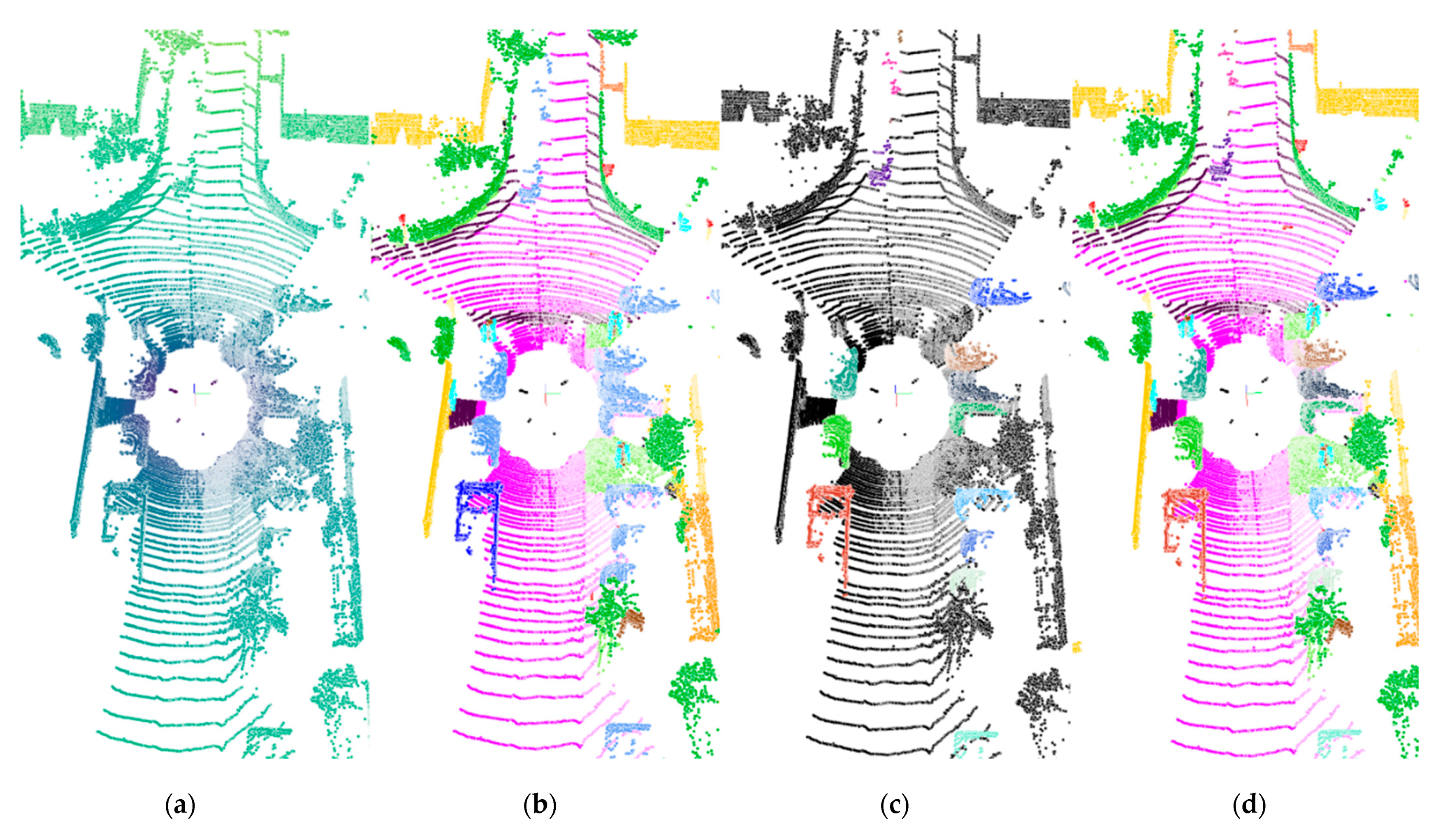
Though panoptic segmentation has garnered extensive attention in the image domain, it is still in its infancy for point cloud processing. Depending on the scene and the sensor, point cloud panoptic segmentation methods can be categorized into indoor RGB-D-based methods and outdoor LiDAR-based methods. As for indoor scenes, some progress has been made in terms of algorithms and benchmark datasets for panoptic segmentation of dense and homogeneous point clouds that are obtained from RGB-D sensors. The typical approach is to voxelize the point clouds and then extract or learn features directly point by point for clustering. However, on the one hand, it is difficult to apply the idea of indoor RGB-D-based methods to outdoor tasks because of sparsity, disorder, and uneven distribution of LiDAR point clouds in outdoor scenes. On the other hand, the small number of LiDAR point cloud datasets with accurate annotation information has constrained otherwise flourishing research on point cloud panoptic segmentation in outdoor scenes. Since LiDAR is less susceptible than vision sensors to light and weather conditions, it is now extensively used in environmental perception applications, such as robotic mapping, autonomous driving, 3D reconstruction, and other areas [3]. To pave way for research on LiDAR-based scene understanding, Behley et al. introduced the SemanticKITTI dataset [7] that provides point-wise annotation of each LiDAR scan in the KITTI dataset. The authors also set up qualification tasks, such as semantic segmentation, panoptic segmentation, semantic scene complementation, and dynamic object segmentation. For clarification, we illustrate panoptic segmentation as well as related tasks using sample data (sequence 08) from SemanticKITTI in Figure 1.
Currently, panoptic segmentation of LiDAR point clouds is achieved by either voxelizing the point clouds (with cubes or cylinders) for 3D convolution [8] or downscaling the point clouds into images for 2D convolution [9]. Voxelization usually yields high accuracy, but its intensive memory consumption and expensive computation cost make it impractical for real-time applications [10]. Downscaled point cloud projections represent each frame as a regular image of the same scale, and a variety of mature 2D image convolution methods are available for panoptic segmentation [11]. Although it is feasible for real-time data processing, the downscaled projection method inevitably loses some information and thus needs accuracy improvement. In general, several recently proposed LiDAR-based panoptic segmentation methods suffer from either low efficiency (resulting from the high computational complexity of point clouds) or low accuracy (due to downscaling point clouds to achieve real-time performance). It seems that efficiency and accuracy cannot be balanced. However, the applications of LiDAR, such as autonomous driving and mobile mapping, require real-time processing of point cloud data. The characteristics of LiDAR point cloud, the realistic need for real-time processing, and the accuracy requirements for scene understanding motivate the research on real-time panoptic segmentation of LiDAR point clouds in this study. In other words, how to improve the accuracy of panoptic segmentation while meeting the requirements of real time is the goal of our research. Specifically, this study proposes a spatiotemporal sequential data fusion strategy based on “thing classes” point fusion and considers that the LiDAR point cloud is sparse, susceptible to occlusion, and distance-dependent (i.e., dense in close range and sparse in far range), thereby yielding high-density data of “thing classes” objects. To meet the real-time requirements, the point cloud was downscaled and projected as a 2D bird’s-eye view (BEV) image and represented in polar coordinates instead of cartesian coordinates. Furthermore, multiscale features were efficiently extracted and aggregated by improving the codec network with UNet as the backbone, called PolarUNet3+. Within the proposed network, semantic and instance branches shared the features for semantic and instance predictions, respectively. Finally, the semantic segmentation predictions were fused with the instance segmentation predictions to remove the ambiguity in point-wise segmentation, thereby yielding panoptic segmentation prediction for a single scan. As for the choice of benchmark dataset, the nuScenes dataset [12] does not provide ground truths for panoptic segmentation, thus the experimental evaluation was performed only with the SemanticKITTI dataset. The experimental results show that our method could achieve an effective balance between accuracy and time efficiency.
The major contributions of this study are as follows:
- (1)
- A data fusion strategy based on “thing classes” points was proposed, which increased the proportion of valuable data in the unbalanced datasets. It could be combined with random sampling to balance the size of input data for training. This data fusion method could alleviate the adverse impact caused by the uneven category distribution of a point cloud. The experiments showed that this pattern was also applicable to other LiDAR point cloud segmentation tasks.
- (2)
- An improved UNet based on polar coordinate representation was used as a strong shared backbone, which could effectively aggregate shallow and deep features at full scales. The polar coordinate representation could minimize the negative impact caused by the inherent “the farther, the sparser” feature of LiDAR point clouds.
2. Related Work
Point cloud segmentation is fundamental to scene understanding, which requires an understanding of both global geometry and a combination of fine-grained features at each point to enable point-wise segmentation. This section presents research work related to semantic, instance, and panoptic segmentation for scene understanding with varying focuses, namely category prediction of environmental elements, object recognition of environmental elements, and an overall understanding of the environment, respectively.
2.1. Semantic Segmentation of Point Clouds
Early semantic segmentation of point clouds usually employed methods such as support vector machines, conditional random fields or random forests, which offered limited semantic annotation classes and low accuracy rates. Deep learning, with its powerful learning capabilities at the feature level, has progressively become the dominant approach for semantic segmentation of point clouds. In terms of application scenarios, point cloud semantic segmentation can be divided into indoor and outdoor applications; segmentation methods can be divided into four types: point convolution, image convolution, voxel convolution, and graph convolution [13]. Point clouds of an indoor scene are usually acquired by RGB-D sensors and characterized by limited spatial coverage, dense data points, and evenly distributed point clouds. For indoor scenes, PointNet [14] and PointNet++ [15], the most representative point convolution methods, extract local feature information for semantic segmentation through multiscale domain information of points. Researchers in [16] voxelized the point cloud to achieve indoor semantic segmentation by extracting aggregated voxel features. In [17], the point cloud was represented as a set of interconnected simple shapes with hyper points and directed graphs with attributes were used to capture the results with contextual information for semantic segmentation. For outdoor scenes, image convolution methods are more often used when real-time performance is considered. This category of methods downscales the 3D point cloud data by projecting them onto a 2D image plane, which is semantically segmented and then projected back onto the 3D data. In [18], images of the point cloud data were captured from all angles, and the 3D data were reduced in a multi-view format, for which the difficulty lays in selecting the viewpoint. Some studies [19,20,21] subjected the point cloud data to spherical projection to yield the range image for semantic segmentation. PolarNet [22] used a projection of the point cloud as a BEV and employed circular convolution to achieve semantic segmentation. If the requirement of real-time is not considered, voxel convolution dominates while rasterizing the point cloud and convolving it in the form of voxels to address the effects of disorder in the point cloud data. 3DCNN-DQN-RNN [23] and VolMap [24] were early works, but their performance was limited by the choice of voxel size and thus needs to be improved. Cylinder3D [25] considered the data distribution characteristics of the LiDAR point cloud, subjected the point cloud to cylindrical partitioning, and applied 3D sparse convolution to yield impressive segmentation performance. Objectively speaking, the characteristic of LiDAR point clouds, “the farther, the sparser”, is still a challenge to the voxel convolution methods.
2.2. Point Cloud Instance Segmentation
Similar to image instance segmentation methods, point cloud instance segmentation methods can be divided into two groups: proposal-based methods and proposal-free methods. Proposal-based methods first perform 3D object detection and then generate instance mask predictions for every object. Three-dimensional semantic instance segmentation (3D-SIS) [26] learns color and geometry features from RGB-D scans to achieve indoor semantic instance segmentation. Generative shape proposal networks (GSPNs) [27] develop a shape-aware module by enforcing geometric understanding to generate proposals. 3D-Bonet [28] formulates the bounding box generation task as an optimization problem and uses two independent branches to generate proposals and mask predictions. Proposal-based methods require multistage training and encounter the challenge of redundant proposals, which make it difficult to obtain real-time instance segmentation results.
Proposal-free methods usually regard instance segmentation as a clustering task based on semantic segmentation, and the research efforts focus on feature learning and clustering of instance points. The similarity group proposal network (SGPN) [29] is a pioneering development in which highly similar points are clustered by constructing a similarity matrix for the learned point features. A variety of instance segmentation methods based on similarity assessment have emerged immediately after that report. Reference [30] described 2D–3D hybrid feature learning based on a global representation of 2D BEVs combined with local point clouds and clustered instance points by using the mean shift algorithm. PointGroup [31] uses 3D sparse convolution to extract semantic information and guides instance generation through the offset prediction branch. As a subsequent clustering step to semantic segmentation, proposal-free methods are usually not computationally intensive, but the accuracy of their instance segmentation is limited by the performance of semantic feature extraction and the effect of sparse point clustering. At this stage, the challenge of the proposal-free methods is to improve the accuracy of instance partitioning while maintaining the efficiency of partitioning.
2.3. Point Cloud Panoptic Segmentation
As for feature extraction, point cloud panoptic segmentation puts semantic segmentation and instance segmentation under a unified framework in accordance with the four segmentation methods (i.e., point convolution, image convolution, voxel convolution, and graph convolution), and the proposal-based or proposal-free methods are used for instance point inference. Building on existing approaches of semantic and instance segmentation, research on panoptic segmentation focuses on aspects such as the disambiguation between semantic and instance predictions and the efficient clustering of instance points. Multiobject panoptic tracking (MOPT) [32] and EfficientLPS [33] downscale point cloud data into distance images for feature extraction and fuse semantic predictions with instance prediction results based on confidence levels to remove point-by-point prediction ambiguities. Panoptic-DeepLab [34] clusters neighboring points according to a prediction of the regression centers of the instances. DSNet [8] incorporates a learnable dynamic shift module based on Cylinder3D [25] to select different bandwidths for clustering sparse instance points. Panoptic-PolarNet is based on PolarNet [22] to downscale point clouds to BEV images to predict regression centers and offsets for real-time panoptic segmentation. Based on KPConv [35], 4D-PLS [5] achieves panoptic segmentation and target tracking by fusing multi-frame point clouds and using a density-based clustering method.
3. Method
Our work was inspired by Panoptic-PolarNet [9] and aimed to achieve improvement from four perspectives: The “thing classes” point data were fused in specific spatial and temporal domains; a robust shared backbone network, namely, Polar-UNet3+, was created by improving the codec network; a parallel semantic segmentation branch and instance segmentation branch were used to generate separate predictions; and finally, the semantic segmentation predictions and instance segmentation predictions were merged to yield the panoptic segmentation results. This section describes in detail the modules and the workflow of our method.
3.1. Overview
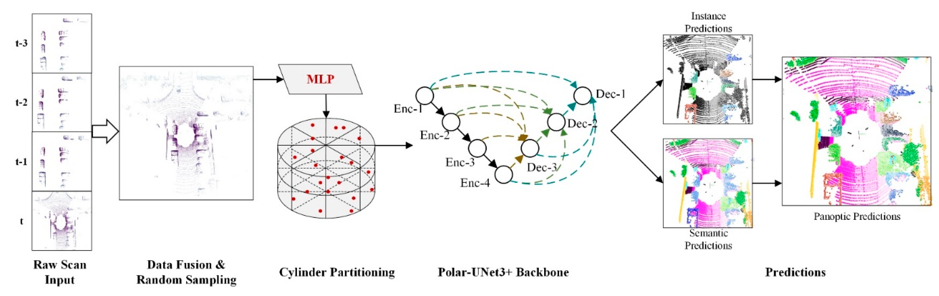
Our method draws on the panoptic segmentation process in Panoptic-PolarNet [9], and the design of each component was inspired by various distinguished methods, which resulted in the methodological framework shown in Figure 2. The spatiotemporal sequential data fusion module enabled the fusion of “thing classes” points in a specific spatiotemporal domain. This module worked with the random sampling module to reduce the amount of data input to the backbone network. The cylindrical partitioning module transformed the point cloud data from a cartesian coordinate representation into a polar coordinate representation and combined the point-wise features obtained through multilayer perceptron (MLP) processing with cylindrical voxelized partitioning to generate the cylindrical partitioning features. The backbone network module obtained a robust backbone network, Polar-UNet3+, by using full-scale skip connections, and the semantic segmentation branch shared the features extracted from the backbone network with the instance segmentation branch to generate predictions. The prediction fusion module fused the panoptic segmentation results using majority voting to eliminate the semantic segmentation ambiguity within instances caused by point-wise segmentation.
3.2. Multi-Scan Fusion via Foreground Point Selection
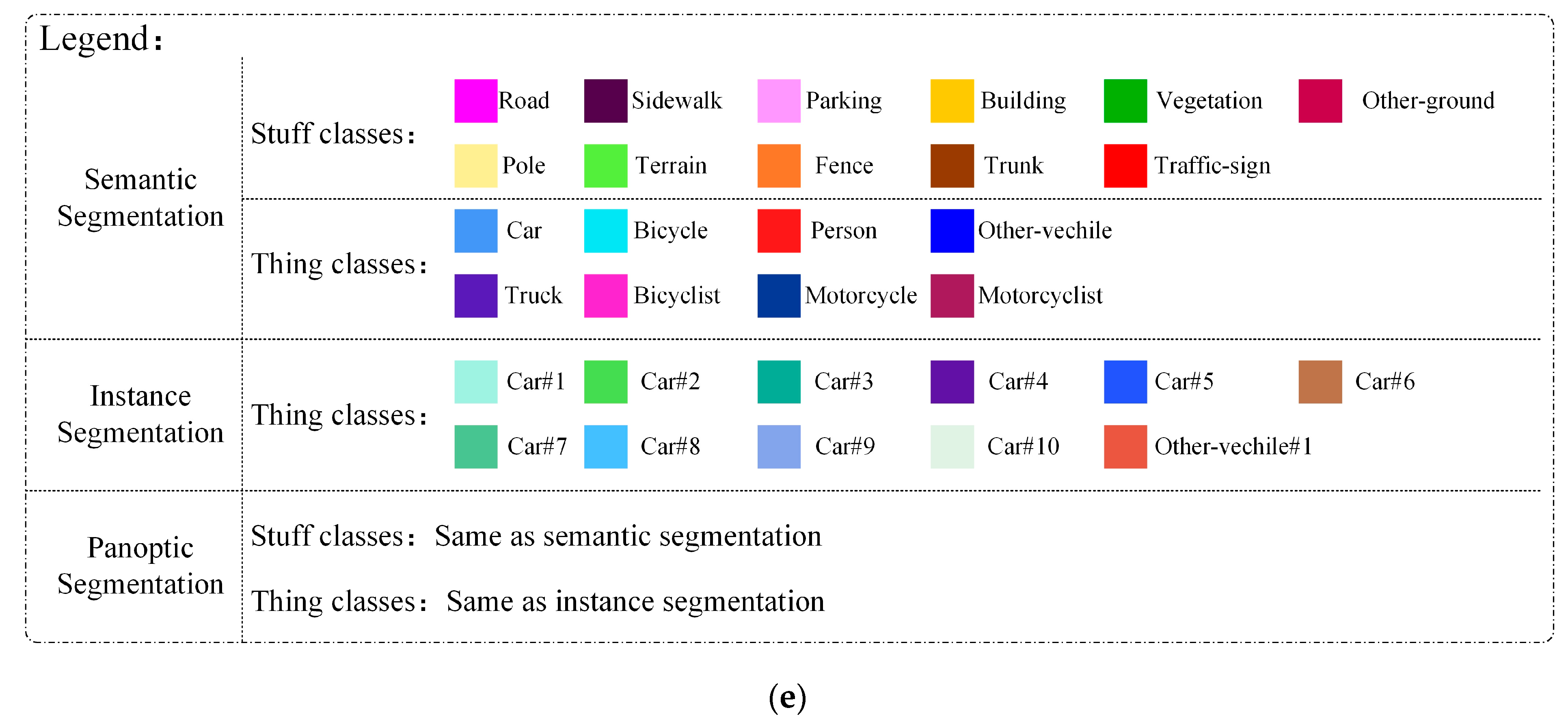
In panoptic segmentation, movable environmental elements are usually assigned to the “thing classes”, and immovable environmental elements are assigned to the “stuff classes”. In the SemanticKITTI dataset, for example, the number of “thing classes” was set to eight (“car”, “truck”, “bicycle”, “motorcycle”, “other-vehicle”, “person”, “bicyclist”, “motorcyclist”), while that of “stuff classes” was set to 11 (‘road”, “sidewalk”, “parking”, “other-ground”, “building”, “vegetation”, “trunk”, “terrain”, “fence”, “pole”, “traffic-sign”). To better analyze the distribution of various environmental elements in a single scan of point cloud data, we sampled every 100 frames in the sequence 00 data and counted the average percentage of various environmental elements in 46 frames of data, as shown in Table 1. (Considering the size of the table, we selected the proportion of 10 frames of data for display and the average proportion of 46 frames of data sampled in the last row.)
As the table shows, the average percentage of environmental elements in the “thing classes” was 8.9%, while the average percentage of environmental elements in the “stuff classes” was 91.1%. It was challenging to achieve accurate instance segmentation of the “thing classes” environmental elements with less than 10% of the data while still meeting real-time requirements. Inspired by the Range Sparse Net (RSN) [36], we proposed a spatiotemporal sequential data fusion strategy based on “thing classes” point fusion to improve the performance of panoptic segmentation by fusing multiple scans of “thing classes” point data to yield a relatively complete portrayal of the “thing classes” of instances. RSN achieves real-time object detection by predicting the “thing classes” points. RSN first downscales the LiDAR point cloud into an image, then segments the “thing classes” points and “stuff classes” points, and finally applies a convolution operation to the chosen “thing classes” points to yield 3D object detection.
As for autonomous driving in urban environments, where LiDAR collects environmental information at a fixed position relative to the vehicle, only part of the instance-level environmental elements can be captured in a single scan of data. In other words, the complete information on the instance-level environmental elements cannot be acquired in a single scan of data. As the position of the LiDAR acquisition changes, multiple views of the environment are continuously collected. By fusing multiple scans of data within a certain time window, theoretically, a relatively complete picture of the instances can be acquired. Our goal was to improve the panoptic segmentation performance by integrating the “thing classes” data in a specific spatial and temporal domain during training. For point cloud data and a time-window threshold for the current moment , we fused the “thing classes” point data located within time window and the point cloud data for the current moment. The fused point cloud data were taken as input for single-frame panoptic segmentation. Point cloud fusion was performed based on the pose description and coordinate transformation method in simultaneous localization and mapping (SLAM). Firstly, each point contained in the point cloud data was represented in the form of a homogeneous coordinate, namely , where is the cartesian coordinate of and is the intensity value. Then, the adjacent frame data were transformed into the same coordinate system for fusion based on the pose description matrix for fusion, where consists of a rotation matrix and a translation vector . The pose description matrix for any two frames of data transformed by coordinates could be expressed as , and the coordinate transformation process could be expressed as . Figure 3 shows a schematic diagram of instance-level point cloud fusion based on multiple scans of data (taking a car as an example).
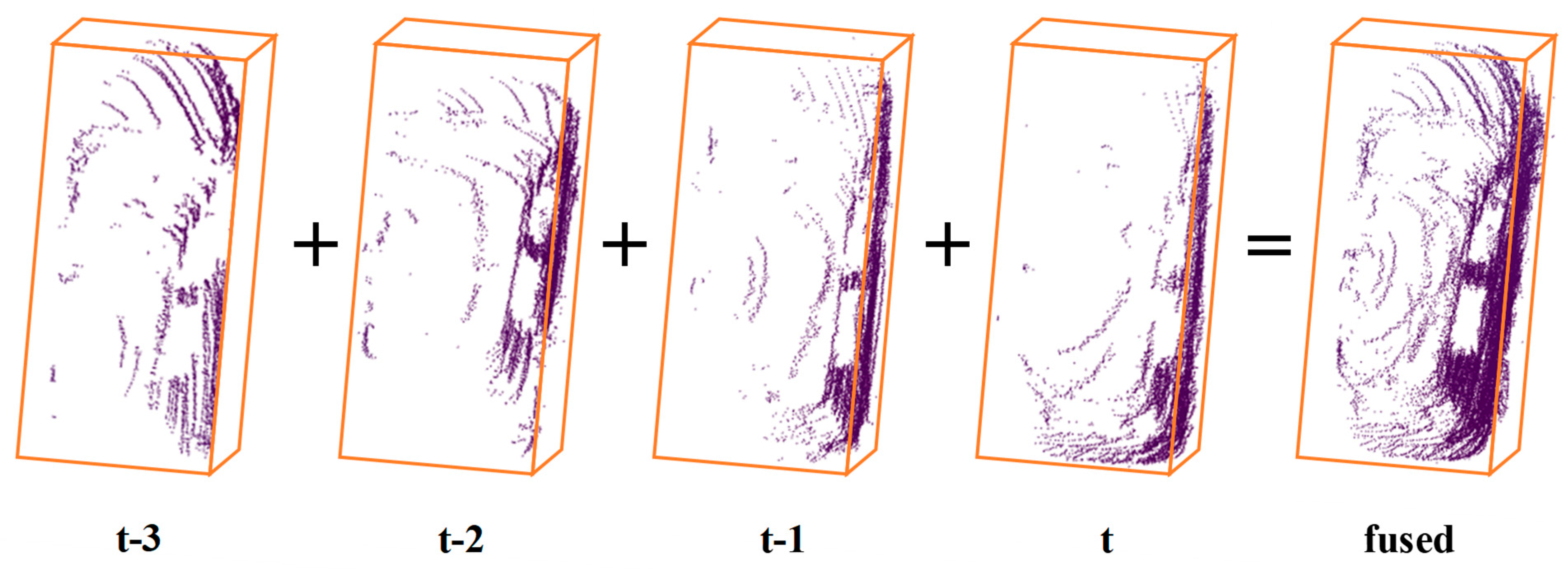
Considering that in the environment there are elements that are either stationary or moving at different speeds, the quality of the point cloud data fusion might be degraded when the “thing classes” elements are moving too fast or when a large time-window threshold is selected. Hence, the time-window threshold was set to 3 in this study. Figure 4 shows a schematic diagram of foreground environmental element point cloud data fusion based on the past three scans.
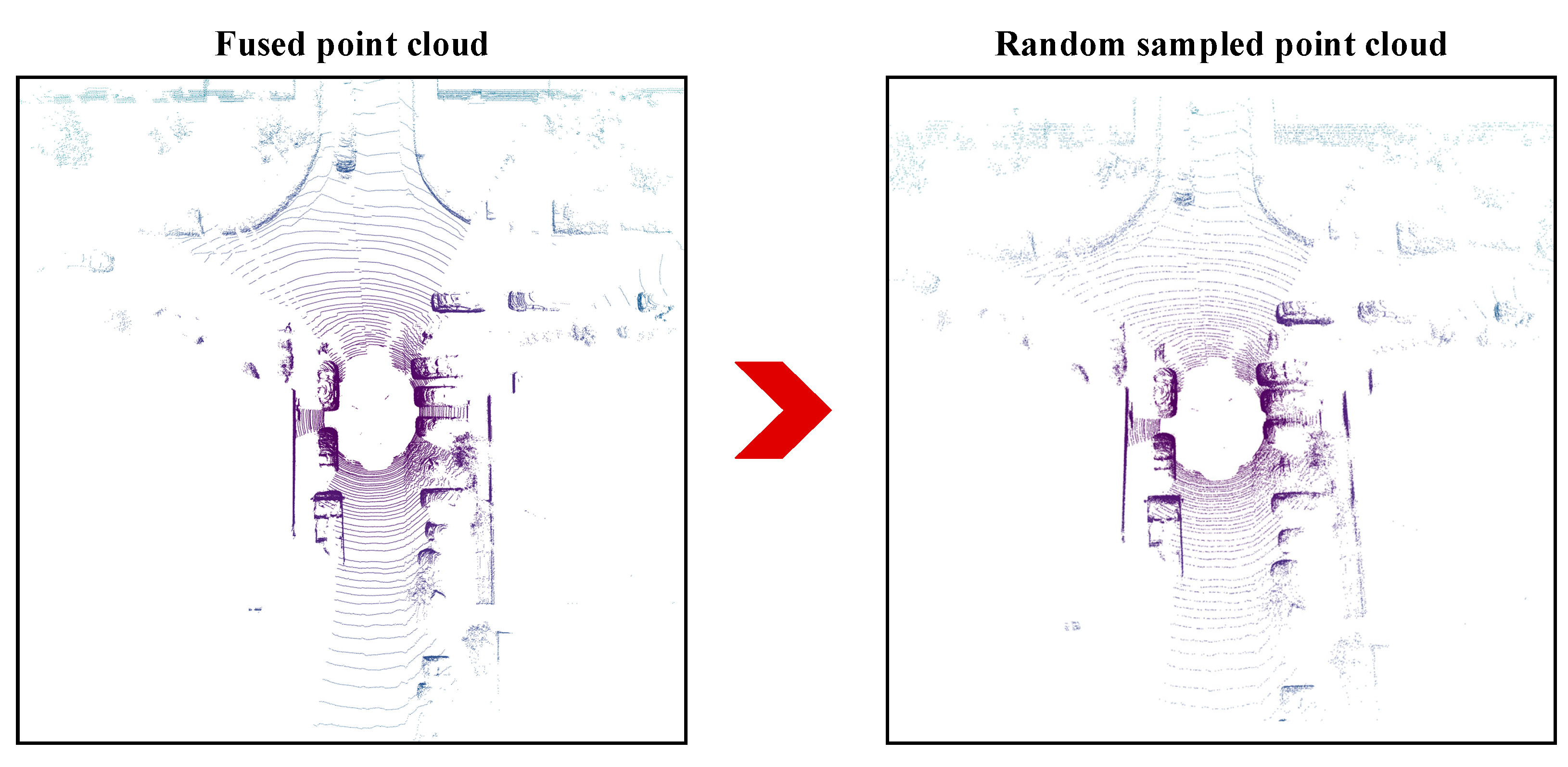
The fusion of multiple scans of “thing classes” point data increased the amount of input data for a single frame during the training, which resulted in an increase of the amount of input data by approximately 10% for each additional frame of “thing classes” point data fused. Moreover, only the current frame could be used in the panoptic segmentation test for single scan data, and it was impossible to fuse multiple frames from the past. To improve the performance and robustness of our approach, we randomly sampled training data after a certain number of epochs of initial training were performed with input data integrated with multiple scans’ “thing classes” points. In other words, the amount of input data that was fused with multiple scans’ “thing classes” points was randomly sampled to a single-frame data size, thereby ensuring that the amount of training data in a single scan was guaranteed to match the amount of validation and test split. Figure 5 shows a schematic diagram of random sampling of the fused point cloud data. The point cloud data became sparse, especially the environmental elements in “stuff” classes with high data proportions (such as roads).
3.3. Polar–Cylindrical Partitioning
When aiming to analyze the characteristics of the LiDAR point clouds, on the one hand, we easily found that if the point cloud was viewed from an overhead perspective, the 2D aerial view showed an approximate circular distribution of point data [22]. However, the LiDAR point cloud also showed a cylindrical distribution centered on the sensor [25]. On the other hand, the inherent “the farther, the sparser” feature of LiDAR point clouds causes the density of point cloud data to be inversely proportional to distance. That is, point density decreases as distance increases. Due to the “the farther, the sparser” feature, the cube-voxelization method that is suitable for homogeneous and dense indoor point clouds is not applicable to outdoor LiDAR point clouds. Based on the cylindrical distribution characteristics of point cloud data and the “the farther, the sparser” feature, PolarNet [22] and Cylinder3D [25] apply cylindrical voxelization of point clouds and achieve semantic segmentation by using two-dimensional convolution and three-dimensional sparse convolution, respectively. We took full advantage of the above-noted research findings and adopted cylindrical partitioning of the point cloud data according to polar coordinates.
With respect to the commonly used regular cubic voxelization method, each equal-sized grid contains significantly fewer data points as the distance increases, while the grids close to the center of the sensor contain more data points. Moreover, the polar coordinate system-based cylindrical voxelization method generates equal-angle sectors of different sizes with varying radii, while the volume of the sector closer to the sensor center is smaller than that of the sector farther away. Compared with conventional voxelization, benefiting from equal-angle division, cylindrical partitioning contains fewer data points in closer grids and more data points in more distant grids. Overall, the point data becomes increasingly evenly distributed within the grid as the distance varies. Each point in the input data at the current moment is transformed into a polar coordinate point by the following function:
After the coordinate transformation, the position of the point in the cylindrical partition is determined based on the point distance , axis radius , and azimuth . Then, the points within each sector in the partition are given a fixed length feature vector by MLP. This vector is used as an input feature for the backbone network.
3.4. Backbone Design
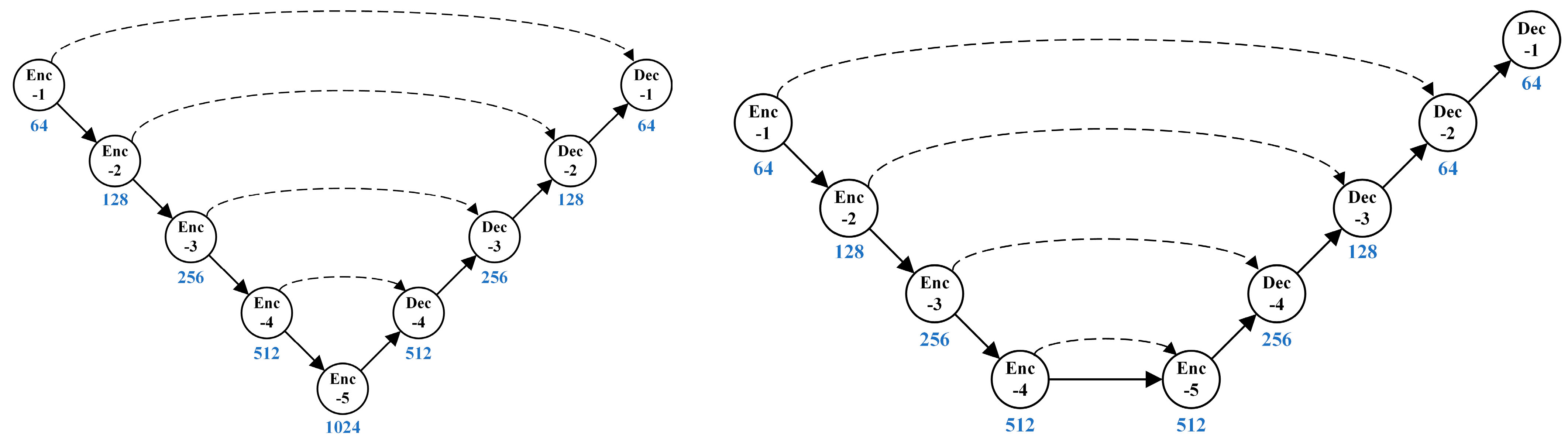
The design of the backbone network is central to achieving fast and accurate panoptic segmentation. Considering the research progress in real-time panoptic segmentation at the current stage, we chose the lightweight and efficient UNet [37] as the infrastructure and considered the contribution of UNet3+ [38] in improving network performance to create our backbone network, Polar-UNet3+. Figure 6 illustrates a schematic comparison of UNet and Panoptic-PolarNet.
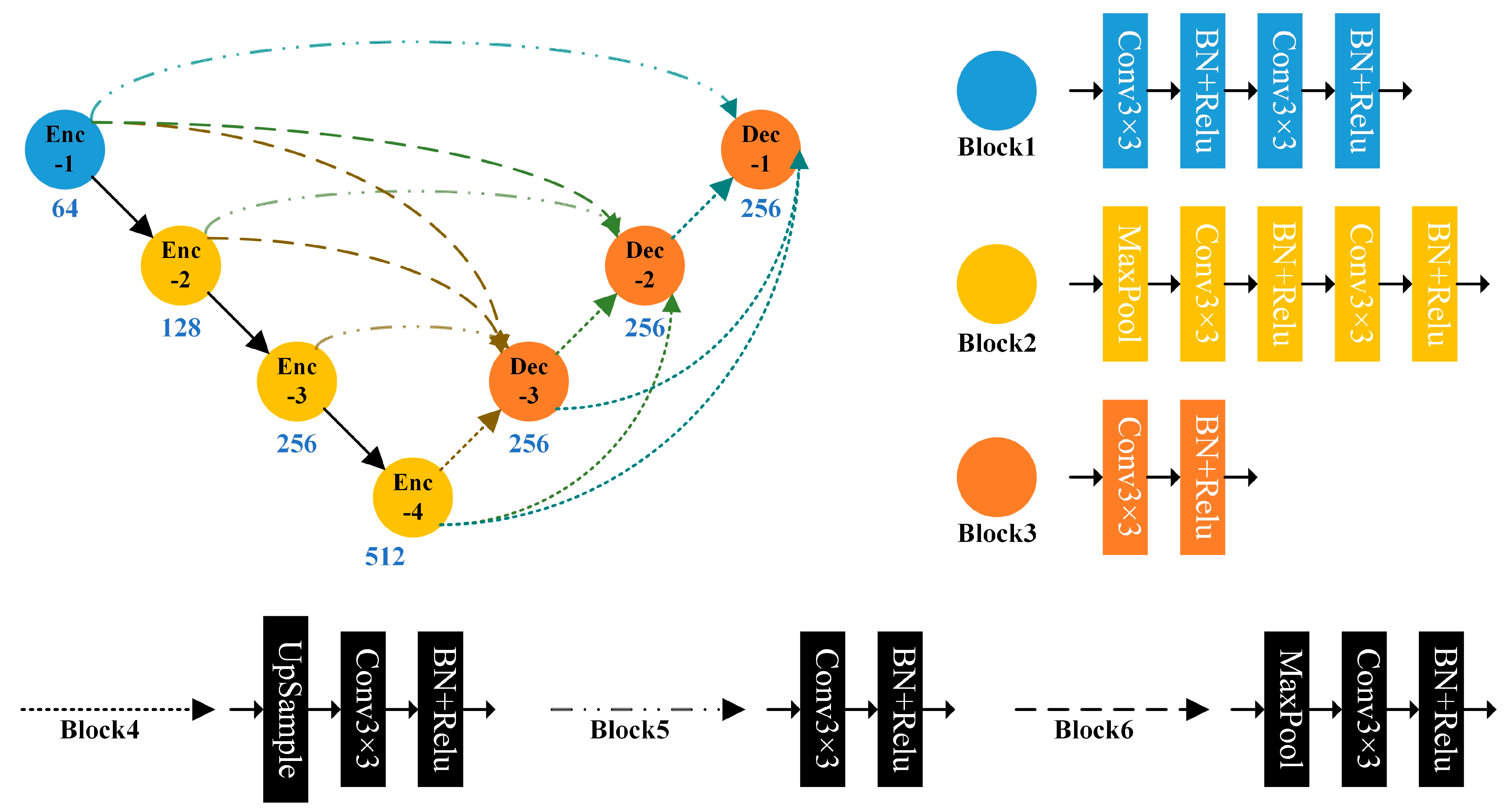
The key concern to network design is the model’s ability to efficiently extract and integrate features at all levels. As a classical “U-type” codec architecture, UNet integrates the features extracted from encoding and decoding sessions by using skip connections; UNet’s idea of feature integration is to integrate deep features upon the completion of coding without paying attention to shallow features. To fully integrate shallow features, UNet++ [39] uses nested joins to integrate shallow features from the first coding round, thereby improving performance, but the nested join approach may impair the real-time performance. UNet3+ goes a step further by using full-scale skip connections instead of nested joins, complemented by a deep supervision strategy. This enables the integration of feature information at full scale, thereby further improving performance while ensuring real-time performance. We proposed Polar-UNet3+ for LiDAR point cloud segmentation based on UNet3+. Polar-UNet3+ consists of four encoders and three decoders. Each decoder integrates multiscale features from the encoder or other decoders by upsampling or maximum pooling, thereby allowing each decoder to gain shallow and deep features at full scale, as shown in Figure 7. In contrast to UNet and Panoptic-PolarNet, Polar-UNet3+ integrates multiscale features through full-scale skip connections.
The features extracted by Polar-UNet3+ are shared by parallel semantic and instance branches. The semantic branches provide point-wise prediction annotations, and the instance branches offer regression centers for prediction instances. In the semantic branch, the unbalanced amount of data containing various environmental elements in the point cloud data poses a challenge for the semantic segmentation of small categories. Each scan contains a significantly higher proportion of “stuff classes” environmental elements than “thing classes” environmental elements. The imbalance in the data frequently causes the semantic segmentation network to tend to learn a high proportion of environmental element categories in training, and it is difficult to fully learn a very low proportion of environmental element categories. To minimize the performance loss of the semantic segmentation network due to the imbalance in the data, we chose a weighted cross-entropy loss function in the semantic branch :
where denotes a weight value that depends on the inverse of the frequency of occurrence of each category of environmental elements, denotes the predicted value for category , and represents the true value for category .
Concerning the instance branch, based on the regression center with comprehensive consideration given to the clustering effect and running time, this study employed the mean shift clustering algorithm to cluster the “thing classes” data points to generate the instance ID. 4D-PLS [5] and Panoptic-PolarNet [9] employ a density clustering algorithm, while DSNet [8] incorporates a dynamic shifting algorithm by improving the mean shift clustering algorithm. Compared with the density clustering algorithm, the mean shift clustering algorithm is less sensitive to density variations and noise points and is thus more suitable for sparse LiDAR point clouds. Moreover, unlike the dynamic shifting algorithm, the mean shift clustering algorithm does not require iterative operations of bandwidth and kernel functions and differentiation operations, thus effectively reducing the clustering time. We first chose the mean squared error loss as the loss function for the regression center prediction in the instance branch and then used the function as the loss function for the instance ID:
In summary, we used the loss function to train Polar-UNet3+:
3.5. Prediction Merging
Ideally, the inner points of the predicted instance ID should have consistent semantic labels. In other words, the same instance ID should share the same semantic label, and the same point should not be assigned to a different instance ID. However, in the class-independent instance segmentation method, it is inevitable that the semantic labels of the inner points of the same instance ID are inconsistent because the clustering of points into instances in the instance branch cannot consider the predicted values of the semantic categories in the semantic branch. To resolve the ambiguity between point-wise semantic annotations and shared instance IDs within each instance, we followed the majority voting strategy in the class-independent panoptic segmentation method to choose the semantic annotation value with the higher percentage of internal points of the same instance as the semantic annotation value of the instance ID, thereby correcting the points with inconsistent semantic annotations. The simple and efficient majority voting strategy ensured consistency between instance segmentation and semantic segmentation with minimal consumption of computational resources.
4. Experiments
In this section, we evaluate our approach on the public dataset SemanticKITTI. We performed the training on a hardware platform with eight GeForce RTX™ 2080 TI graphic processing units (GPUs) (11 GB of video memory) with 80 epochs. After 50 epochs of training, the random sampling strategy was applied. After all training, validation and testing were performed with a single graphics card after training.
4.1. Dataset and Metrics
To fully evaluate the performance of our method and to benchmark it against other panoptic segmentation algorithms, the SemanticKITTI dataset was chosen in this study for training validation and testing. The SemanticKITTI dataset provided 43,442 frames of point cloud data (sequences 00–10 were point cloud ground truths with point-wise annotations). Moreover, challenges for multiple segmentation tasks were launched at the dataset’s official website, where participants’ methods were assessed with uniform metrics. In reference to the requirements on the use of other algorithms and datasets, 19,130 frames of point cloud data from sequences 00–07 and 09–10 were used as the training dataset, 4071 frames of data from sequence 08 were used as the validation dataset, and 20,351 frames of point cloud data from sequences 11–21 were used as the test dataset. For the semantic segmentation and panoptic segmentation of single-frame data, 19 categories needed to be labeled. For the semantic segmentation of multiple scans, 25 categories needed to be annotated (six additional mobile categories). The evaluation metrics for semantic segmentation were mean intersection-over-union (mIoU):
where denotes the number of categories, denote true positive, false positive, and false negative values for category , respectively.
The evaluation metrics for panoptic segmentation [6,40] were the panoptic quality, recognition quality, and semantic quality, denoted as PQ, RQ, and SQ, respectively, for all categories; PQTh, SQTh, and RQTh, respectively, for the “thing classes”; and PQSt, SQSt, and RQSt, respectively, for the “stuff classes”. Additionally, only SQ was used as PQ† for PQ in the “stuff classes”. PQ, RQ, and SQ were defined as follows:
4.2. Performance and Comparisons
Table 2 presents the results of the quantitative evaluation of the method proposed in this study on the test dataset. We took FPS = 10 Hz as the grouping criterion to compare the panoptic segmentation performance of each algorithm to verify the effectiveness of the method proposed in this study. Note that the results of the comparison methods were obtained from the competition, and taking 10 Hz as the grouping criterion complied with the data acquisition frequency, which is usually used as the criterion of real-time performance.
Panoptic-PolarNet uses cylindrical partitioning for instance segmentation with UNet as the backbone network, 4D-PLS adopts multi-scan data fusion to achieve panoptic segmentation of single-scan data, and DS-Net applies 3D sparse convolution of cylindrical partitioning and the dynamic shifting clustering algorithm with multiple iterations. The method proposed in this study drew to varying degrees on these three panoptic segmentation methods. Compared with Panoptic-PolarNet, our approach improved PQ by 0.5% and FPS by 1 Hz. Compared with 4D-PLS, our approach improved PQ by 4.3%. The PQ obtained by DS-Net is 1.3% higher than that obtained by our method, but the FPS obtained by DS-Net is merely 3.4 Hz, which does not allow for real-time panoptic segmentation.
Furthermore, we investigated the key components for performance improvements based on the experiment results. As discussed in the related work (Section 2), a robust panoptic segmentation can be realized using either a strong backbone, excellent clustering methods, or smart data fusion strategies. Firstly, based on the powerful backbone named Cylinder3D, DS-Net proposes a dynamic shifting clustering method to improve the performance of panoptic segmentation. Cylinder3D adopts 3D sparse convolution and obtains a 67.8% mIoU score in single scan semantic segmentation competitions. Therefore, DS-Net can get a 55.9% PQ score. However, our backbone only got less than a 60% mIoU score in single scan semantic segmentation competitions. Thanks to the way of “thing classes” data fusion, we could approach the performance of DS-Net under the condition of meeting the requirements of real time. Secondly, 4D-PLS performs panoptic segmentation by fusing multi-scan data. Although multi-scan data are fused, the proportion of “thing classes” data remains unchanged. In our method, only the “thing classes” data were fused, which improved the proportion of valuable data for instance segmentation, and then improved the performance of panoptic segmentation. Finally, compared with Panoptic-PolarNet, our method adopted a strong backbone that could aggregate features at full scales, called Polar-UNet3+, which could achieve better performance in the case of shortening the panoptic segmentation time.
Table 3 shows, on a semantic category-by-semantic category basis, the quantitative evaluation results obtained by our proposed method on the test dataset. The quantitative evaluation results demonstrate that this method achieved a balance between accuracy and efficiency in panoptic segmentation.
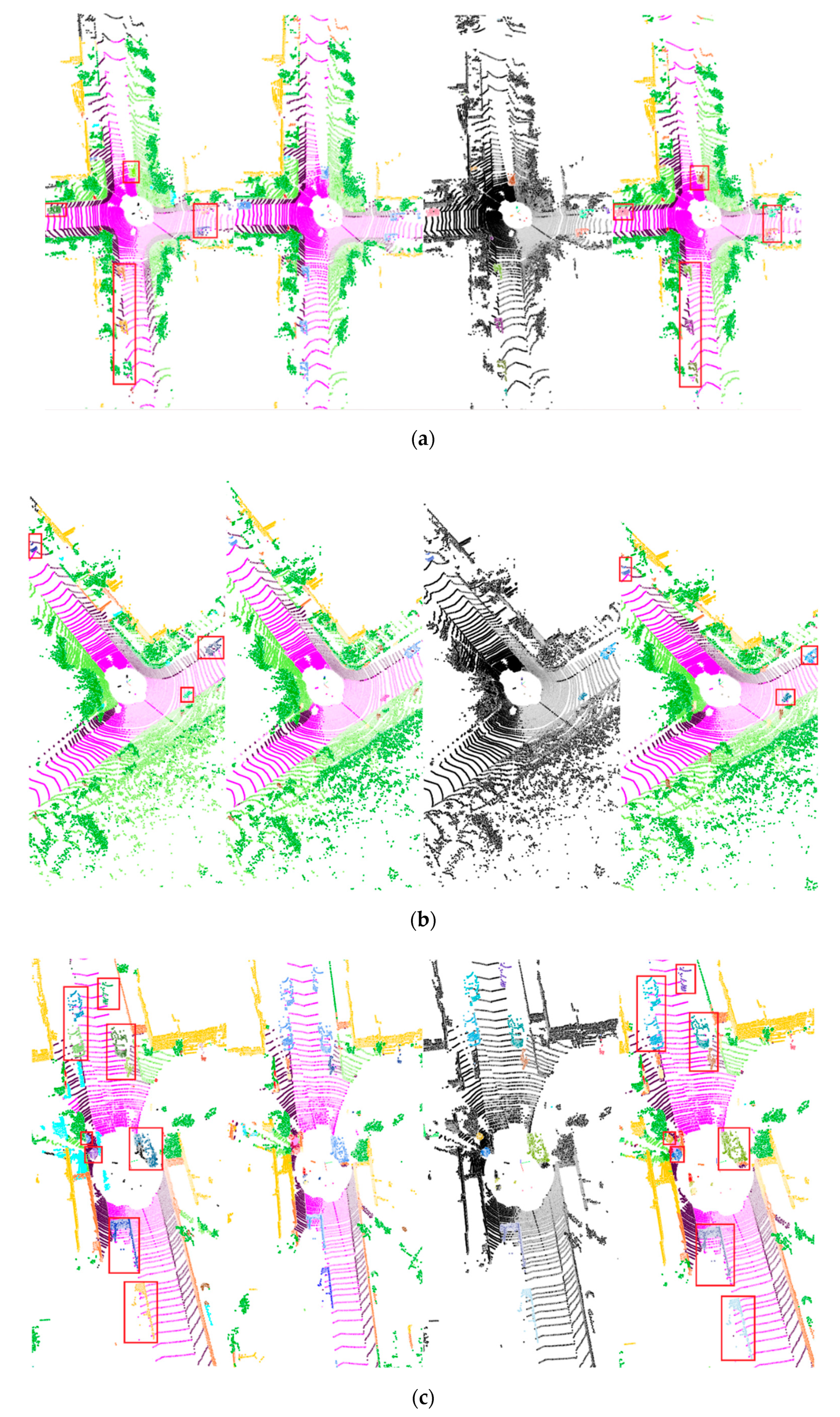
The visualizations of panoptic segmentation results on the validation split of SemanticKITTI are shown in Figure 8. The figure consists of five subfigures, which correspond to the panoptic segmentation results of the five scanned frames sampled at 800-frame intervals in the validation split. Each subfigure consists of four parts: the ground truth of the panoptic segmentation, the semantic segmentation predictions, the instance segmentation predictions, and the panoptic segmentation predictions. Note that we used semantic-kitti-api [44] to visualize the panoptic ground truths and predicted labels. During each visualization, the color corresponding to each instance was given randomly. Therefore, in Figure 8, each instance’s color of the ground truths and predicted labels is inconsistent. The qualitative comparison results show that we could accurately predict each instance and that the error mainly came from the point-wise annotations inside the instance, which will be a direction of improvement in the future.
The visualization results of panoptic segmentation on the test split of SemanticKITTI are shown in Figure 9. The figure consists of eleven subfigures, which correspond to the panoptic segmentation results of each sequence sampled at the 500th scan in the test split (since the 500th scan of sequence 16 contained only a few pedestrians and sequence 17 only had 491 scans, the 300th scan was selected in sequence 16–17). Each subfigure consists of four parts: the raw scan, the semantic segmentation predictions, the instance segmentation predictions, and the panoptic segmentation predictions. Because the test split did not provide ground truths for comparison, we did not use red rectangular boxes for identification.
4.3. Ablation Study
We present an ablation analysis of our approach, which considers the “thing classes” point cloud fusion, random sampling, Polar-Unet3+, and grid size. All results were compared on the validation set, sequence 08. Firstly, we set the grid size to (480, 360, 32) and investigated the contribution of each key component of the method. The results are shown in Table 4. As a key part of the performance improvement, Polar-Unet3+ boosted PQ by 0.8%, a further 0.9% performance improvement was achieved for the “thing classes” point fusion, and the random sampling module improved the stability of the method.
After analyzing the performance of each component, we explored the effect of voxelization size on segmentation time and performance, and the results are shown in Table 5. For the LiDAR point cloud featuring “dense in close range and sparse in far range”, finer voxels did not deliver significant performance gains but rather compromised segmentation efficiency.
4.4. Other Applications
The improvement of panoptic segmentation performance benefited from the “thing classes” data fusion and random sampling strategies. To fully evaluate the effectiveness and generalization of our method, we chose the more challenging semantic segmentation task and the moving object semantic segmentation task to verify our method. The semantic segmentation of moving objects involves training on the basis of multiple scans as input and labeling the semantic on a single scan (the environmental elements of 25 categories need to be predicted, and the environmental elements of specific categories need to be distinguished whether they are moving or not). Compared with moving object segmentation, moving object semantic segmentation not only distinguishes the state of environmental elements (moving or static) but also needs to accurately label all environmental elements. Compared with the semantic segmentation of a single scan, moving object semantic segmentation adds six categories: moving car, moving truck, moving other vehicle, moving person, moving bicyclist, and moving motorcyclist.
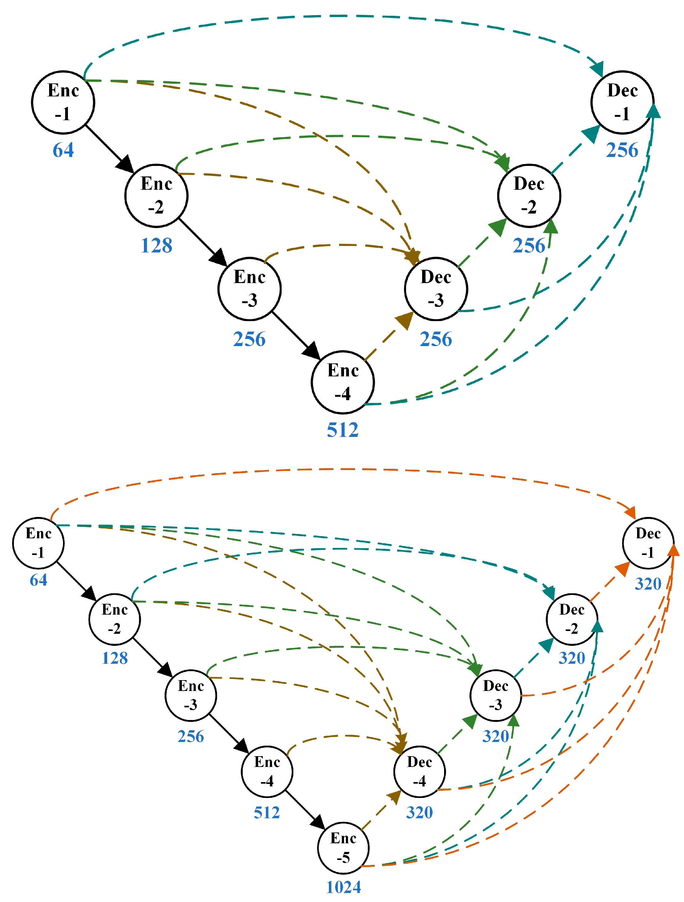
On the basis of ensuring real-time performance, we expanded Polar-Unet3+ for panoptic segmentation, including four encoders and three decoders, to MS-Polar-Unet3+, including five encoders and four decoders. The main reason for deepening the network was that semantic segmentation does not need to predict the instance ID, and the reduced amount of calculation can be used to deepen the network structure, as shown in Figure 10.
In the process of multiple-scan fusion, we defined “thing classes data” as moving-class data, including “moving car”, “moving truck”, “other moving vehicle”, “moving person”, “moving bicyclist”, and ‘moving motorcyclist”. In addition, “1 + P + M” was used to represent the multiple-scan fusion mode, in which P is the number of complete previous scans and M is the number of scans in which only moving-class points are fused. In the selection of P, due to the limitation of the hardware platform, it was difficult for us to integrate the past four scans, as in SemanticKITTI [7], and we set P to 2. In the selection of M, because the number of points in the moving classes accounts for a small proportion, we referred to the conclusion in Lidar-MOS [45] and set M to 8. In the training process, referring to the training parameter setting of the panoptic segmentation task, the grid size was (480, 360, 32), the number of training epochs was 80, and the random sampling strategy was applied at the 50th epoch.
Table 6 shows the quantitative evaluation results of our method on the test split of SemanticKITTI. Our method could obtain 52.9% mIoU on the basis of ensuring real-time performance. The moving object semantic segmentation results of Cylinder3D [25] come from the official evaluation website of SemanticKITTI [46], and we could not confirm its fusion quantity. Note that the existence of moving objects improves the difficulty of semantic segmentation. Cylinder3D [25] obtains 67.8% mIoU in a single scan semantic segmentation task, while it obtains only 52.5% mIoU in a multiple-scan semantic segmentation task. Our method obtained 52.9% mIoU on the basis of ensuring real-time performance.
The quantitative evaluation results of our proposed approach in panoptic segmentation and moving object semantic segmentation on the test split of SemanticKITTI show that our method achieved an effective balance between segmentation accuracy and efficiency, and the foreground data fusion and random sampling strategies could be popularized and applied to other LiDAR-based point cloud segmentation networks.
Furthermore, we combined the segmentation results of dynamic objects with SLAM to evaluate the effectiveness of our method. Moving objects in the environment will produce a wrong data association effect, which will affect the pose estimation accuracy of SLAM algorithms. If moving objects can be removed accurately, it will undoubtedly improve the performance of SLAM algorithms. We chose the MULLS [47] as the SLAM benchmark. We used three kinds of input data for experiments: raw scan, the scan which filtered out dynamic objects according to the semantic ground truth (abbreviated as Dynamic Moving GT), and the scan which filtered out dynamic objects according to the semantic predictions obtained by our method (abbreviated as Dynamic Moving).
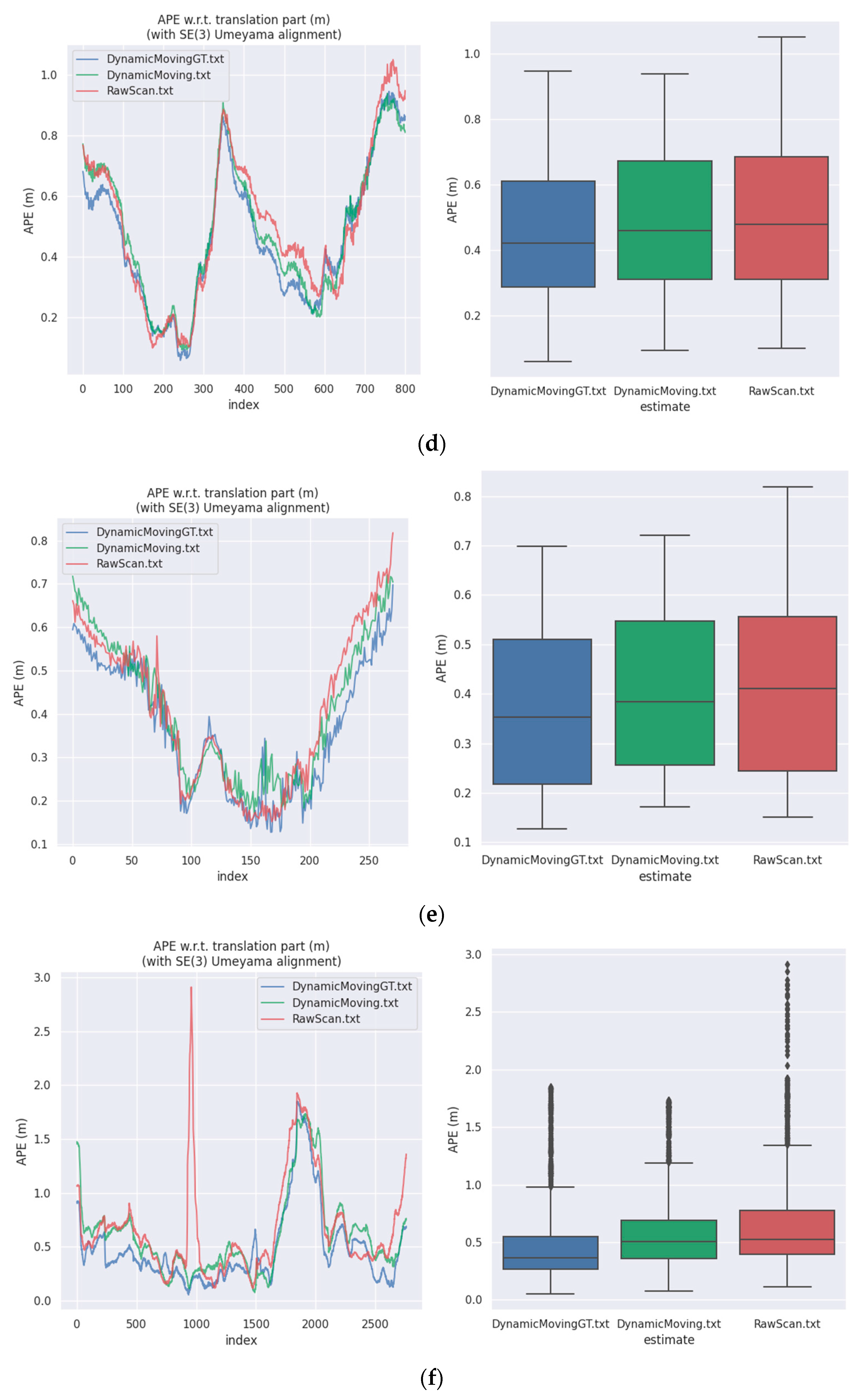
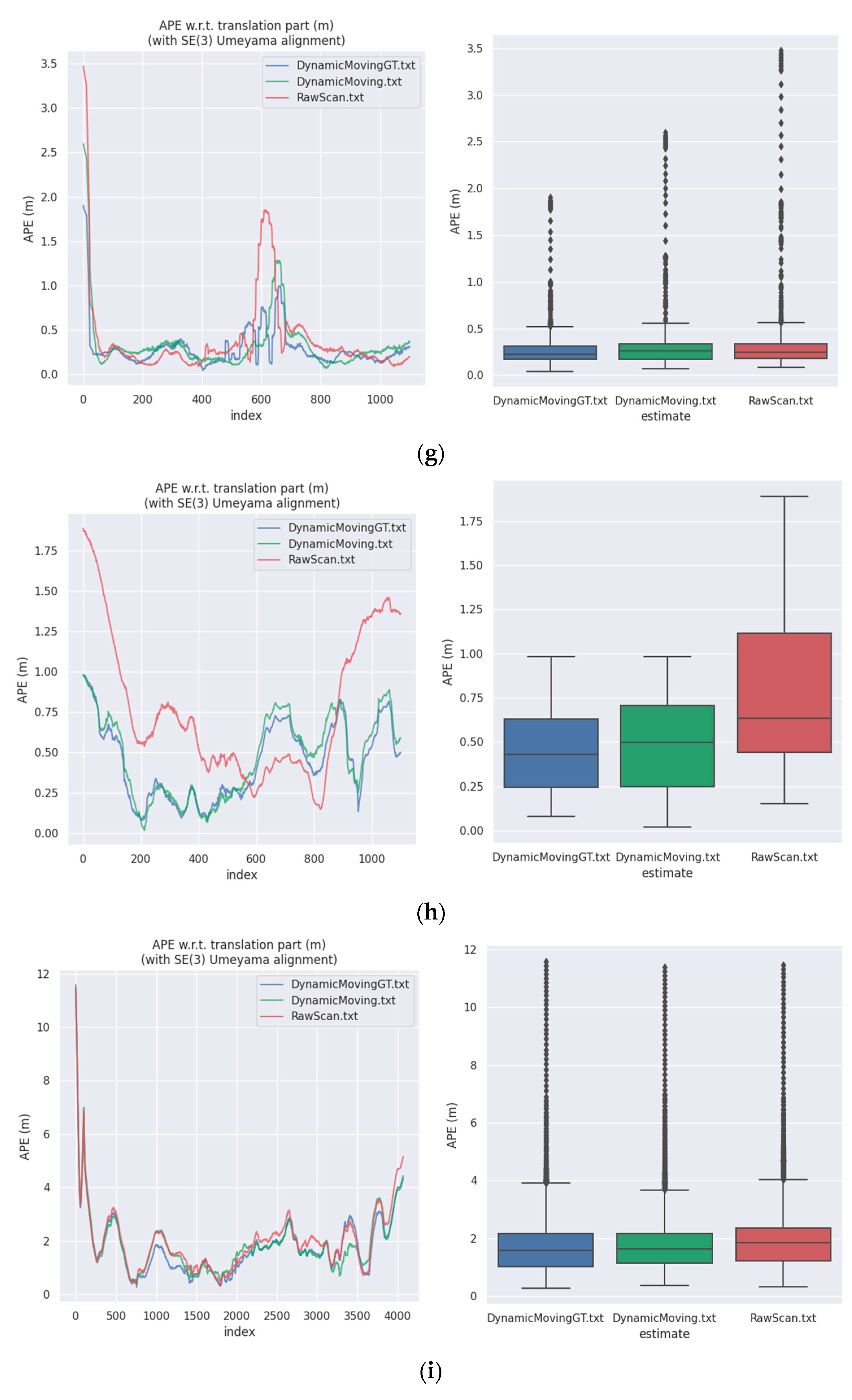
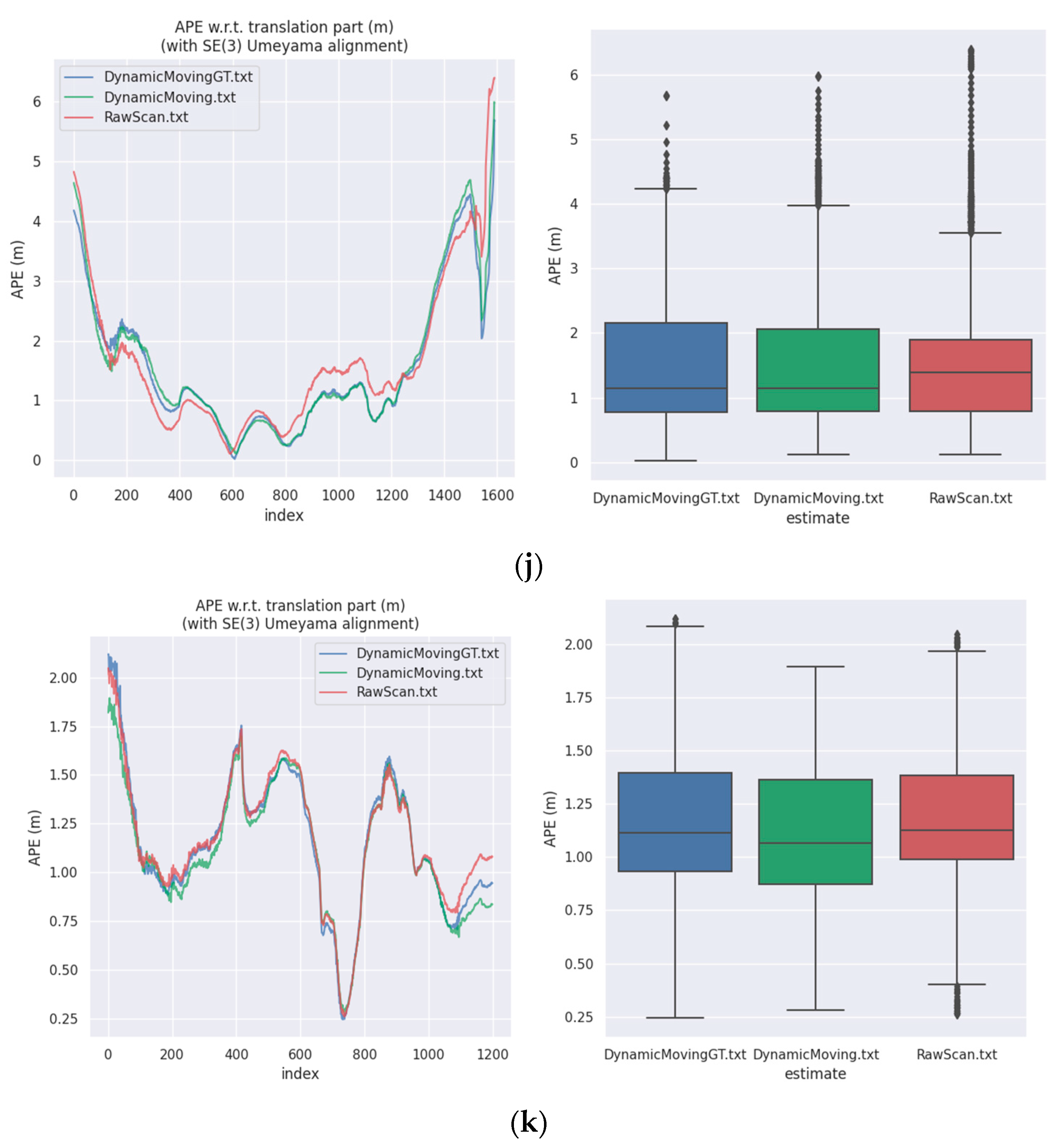
For the evaluation of the SLAM algorithm, the quantitative evaluation index of absolute pose error (APE) was applied, using Sim (3) Umeyama alignment in the calculation. We then used the evo tool [48] to evaluate the estimated pose results, including the root mean square error (RMSE), the mean error, the median error, and the standard deviation (Std.). Table 7 is a comparison of the APE used for the translation component of different inputs based on the MULLS. Figure 11 shows the APE visualization results for different inputs. This figure consists of eleven subfigures, which correspond to the sequence 00–10 in the SemanticKITTI dataset, respectively. According to Table 7 and Figure 10, it is obvious that filtering out dynamic objects could significantly improve the accuracy of pose estimation. Considering that most of the dynamic objects in the KITTI dataset were static in the environment, the experimental results strongly demonstrate the effectiveness of our method in segmenting dynamic objects, which improved the accuracy of pose estimation and enhanced the performance of different SLAM algorithms.
5. Conclusions
This study contributes to achieving fast and accurate scene understanding for autonomous driving in urban environments. Specifically, this study proposes a spatiotemporal sequential data fusion strategy based on the statistical analysis of the characteristics of LiDAR point cloud data. This strategy improved the segmentation performance of “thing classes” fusion while incorporating only a few valuable data points and allowed control of the training input by random sampling. Moreover, this strategy greatly mitigated the adverse effects caused by the uneven distribution of categories caused by the inherent characteristics of urban environment in the limited training data. We believe that this strategy is also applicable to other LiDAR point cloud segmentation tasks. The codec network was further improved by establishing full-scale skip connections to efficiently aggregate the multiscale features shared by semantic and instance branches and to enable accurate panoptic segmentation of a single scan in the consistency fusion module.
To evaluate the proposed method, the SemanticKITTI dataset with point-wise annotations of semantic and instance information was chosen for the experimentation. Experimental results on the SemanticKITTI dataset suggest that our proposed method could achieve an effective balance between accuracy and efficiency. To summarize, this study is an active exploration into the research on scene understanding for intelligent robots with real-time panoptic segmentation of LiDAR point clouds as the core. In the future, we will focus on the fast and accurate scene understanding of complex dynamic environments.
Author Contributions
Conceptualization, W.W. and X.Y.; formal analysis, W.W., X.Y. and J.Y.; methodology, W.W., X.Y., J.Y. and M.S.; software, W.W., L.Z., Z.Y. and Y.K.; supervision, J.Y.; validation, M.S.; writing—original draft, W.W., Z.Y. and Y.K.; writing—review and editing, X.Y., J.Y. and L.Z. All authors have read and agreed to the published version of the manuscript.
Funding
This research was funded by the National Natural Science Foundation of China (Project No.42130112 and No.42171456), the Youth Program of the National Natural Science Foundation of China (Project No.41901335 and No.41801317), the Central Plains Scholar Scientist Studio Project of Henan Province, and the National Key Research and Development Program of China (Project No.2017YFB0503503).
Institutional Review Board Statement
Not applicable.
Informed Consent Statement
Not applicable.
Data Availability Statement
Our experimental data are all open-source datasets.
Conflicts of Interest
The authors declare no conflict of interest.
References
- Gao, J. The 60 Anniversary and Prospect of Acta Geodaetica et Cartographica Sinica. Acta Geod. Cartogr. Sin. 2017, 46, 1219–1225. [Google Scholar]
- Li, D.; Hong, Y.; Wang, M.; Tang, L.; Chen, L. What can surveying and remote sensing do for intelligent driving? Acta Geod. Cartogr. Sin. 2021, 50, 1421–1431. [Google Scholar]
- Wang, W.; You, X.; Zhang, X.; Chen, L.; Zhang, L.; Liu, X. LiDAR-Based SLAM under Semantic Constraints in Dynamic Environments. Remote Sens. 2021, 13, 3651. [Google Scholar] [CrossRef]
- Guo, Y.; Wang, H.; Hu, Q.; Liu, H.; Liu, L.; Bennamoun, M. Deep Learning for 3D Point Clouds: A Survey. IEEE Trans. Pattern Anal. Mach. Intell. 2021, 43, 4338–4364. [Google Scholar] [CrossRef]
- Aygün, M.; Ošep, A.; Weber, M.; Maximov, M.; Stachniss, C.; Behley, J.; Leal-Taixé, L. 4D Panoptic LiDAR Segmentation. In Proceedings of the IEEE/CVF Conference on Computer Vision and Pattern Recognition, Nashville, TN, USA, 20–25 June 2021; pp. 5527–5537. [Google Scholar]
- Kirillov, A.; He, K.; Girshick, R.; Rother, C.; Dollár, P. Panoptic segmentation. In Proceedings of the IEEE/CVF Conference on Computer Vision and Pattern Recognition, Long Beach, CA, USA, 15–20 June 2019; pp. 9404–9413. [Google Scholar]
- Behley, J.; Garbade, M.; Milioto, A.; Quenzel, J.; Behnke, S.; Stachniss, C.; Gall, J. Semantickitti: A dataset for semantic scene understanding of lidar sequences. In Proceedings of the IEEE/CVF International Conference on Computer Vision, Seoul, Korea, 27 October–2 November 2019; pp. 9297–9307. [Google Scholar]
- Hong, F.; Zhou, H.; Zhu, X.; Li, H.; Liu, Z. Lidar-based panoptic segmentation via dynamic shifting network. In Proceedings of the IEEE/CVF Conference on Computer Vision and Pattern Recognition, Nashville, TN, USA, 20–25 June 2021; pp. 13085–13094. [Google Scholar]
- Zhou, Z.; Zhang, Y.; Foroosh, H. Panoptic-PolarNet: Proposal-free LiDAR Point Cloud Panoptic Segmentation. In Proceedings of the IEEE/CVF Conference on Computer Vision and Pattern Recognition, Nashville, TN, USA, 20–25 June 2021; pp. 13189–13198. [Google Scholar]
- Ryan, R.; Ran, C.; Enxu, L.; Ehsan, T.; Yuan, R.; Liu, B. Gp-s3net: Graph-based panoptic sparse semantic segmentation network. In Proceedings of the IEEE/CVF International Conference on Computer Vision (ICCV), Montreal, QC, Canada, 10–17 October 2021; pp. 16076–16085. [Google Scholar]
- Milioto, A.; Behley, J.; Mccool, C.; Stachniss, C. LiDAR Panoptic Segmentation for Autonomous Driving. In Proceedings of the 2020 IEEE/RSJ International Conference on Intelligent Robots and Systems (IROS), Las Vegas, NV, USA, 24 October–24 January 2021; pp. 8505–8512. [Google Scholar]
- Caesar, H.; Bankiti, V.; Lang, A.H.; Vora, S.; Liong, V.; Xu, Q.; Krishnan, A.; Pan, Y.; Baldan, G.; Beijbom, O. nuscenes: A multimodal dataset for autonomous driving. In Proceedings of the IEEE/CVF Conference on Computer Vision and Pattern Recognition, Seattle, WA, USA, 13–19 June 2020; pp. 11618–11628. [Google Scholar]
- Gao, B.; Pan, Y.; Li, C.; Geng, S.; Zhao, H. Are We Hungry for 3D LiDAR Data for Semantic Segmentation? A Survey of Datasets and Methods. IEEE Trans. Intell. Transp. Syst. 2021, 1–19. [Google Scholar] [CrossRef]
- Charles, R.Q.; Su, H.; Kaichun, M.; Guibas, L. Pointnet: Deep learning on point sets for 3d classification and segmentation. In Proceedings of the IEEE Conference on Computer Vision and Pattern Recognition, Honolulu, HI, USA, 21–26 July 2017; pp. 77–85. [Google Scholar]
- Charles, R.Q.; Li, Y.; Su, H.; Leonidas, J. PointNet++ deep hierarchical feature learning on point sets in a metric space. In Proceedings of the 31st International Conference on Neural Information Processing Systems, Long Beach, CA, USA, 4–9 December 2017; pp. 5105–5114. [Google Scholar]
- Choy, C.; Gwak, J.Y.; Savarese, S. 4D spatio-temporal convnets: Minkowski convolutional neural networks. In Proceedings of the IEEE/CVF Conference on Computer Vision and Pattern Recognition, Long Beach, CA, USA, 15–20 June 2019; pp. 3070–3079. [Google Scholar]
- Landrieu, L.; Simonovsky, M. Large-scale point cloud semantic segmentation with superpoint graphs. In Proceedings of the IEEE/CVF Conference on Computer Vision and Pattern Recognition, Salt Lake City, UT, USA, 18–23 June 2018; pp. 4558–4567. [Google Scholar]
- Lawin, F.J.; Danelljan, M.; Tosteberg, P.; Bhat, G.; Khan, F.; Felsberg, M. Deep projective 3D semantic segmentation. In Proceedings of the International Conference on Computer Analysis of Images and Patterns, Ystad, Sweden, 22–24 August 2017; pp. 95–107. [Google Scholar]
- Xu, C.; Wu, B.; Wang, Z.; Vajda, P.; Keutzer, K.; Tomizuka, M. Squeezesegv3: Spatially-adaptive convolution for efficient point-cloud segmentation. In Proceedings of the European Conference on Computer Vision, Glasgow, UK, 23–28 August 2020; pp. 1–19. [Google Scholar]
- Milioto, A.; Vizzo, I.; Behley, J.; Stachniss, C. Rangenet++: Fast and accurate lidar semantic segmentation. In Proceedings of the 2019 IEEE/RSJ International Conference on Intelligent Robots and Systems (IROS), Macau, China, 3–8 November 2019; pp. 4213–4220. [Google Scholar]
- Cortinhal, T.; Tzelepis, G.; Aksoy, E.E. SalsaNext: Fast, uncertainty-aware semantic segmentation of LiDAR point clouds. In Proceedings of the International Symposium on Visual Computing, San Diego, CA, USA, 5–7 October 2020; pp. 207–222. [Google Scholar]
- Zhang, Y.; Zhou, Z.; David, P.; Yue, X.; Xi, Z.; Gong, B.; Foroosh, H. Polarnet: An improved grid representation for online lidar point clouds semantic segmentation. In Proceedings of the IEEE/CVF Conference on Computer Vision and Pattern Recognition, Seattle, WA, USA, 13–19 June 2020; pp. 9598–9607. [Google Scholar]
- Liu, F.; Li, S.; Zhang, L.; Zhou, C.; Ye, R.; Wang, Y.; Lu, J. 3DCNN-DQN-RNN: A deep reinforcement learning framework for semantic parsing of large-scale 3D point clouds. In Proceedings of the IEEE International Conference on Computer Vision (ICCV), Venice, Italy, 22–29 October 2017; pp. 5679–5688. [Google Scholar]
- Radi, H.; Ali, W. VolMap: A Real-time Model for Semantic Segmentation of a LiDAR surrounding view. arXiv 2019, arXiv:1906.11873. [Google Scholar]
- Zhu, X.; Zhou, H.; Wang, T.; Hong, F.; Ma, Y.; Li, W.; Li, H.; Lin, D. Cylindrical and asymmetrical 3d convolution networks for lidar segmentation. In Proceedings of the IEEE/CVF Conference on Computer Vision and Pattern Recognition, Nashville, TN, USA, 20–25 June 2021; pp. 9934–9943. [Google Scholar]
- Hou, J.; Dai, A.; Nießner, M. 3D-SIS: 3D Semantic Instance Segmentation of RGB-D Scans. In Proceedings of the IEEE/CVF Conference on Computer Vision and Pattern Recognition, Long Beach, CA, USA, 15–20 June 2019; pp. 4416–4425. [Google Scholar]
- Yi, L.; Zhao, W.; Wang, H.; Sung, M.; Guibas, L. GSPN: Generative Shape Proposal Network for 3D Instance Segmentation in Point Cloud. In Proceedings of the IEEE/CVF Conference on Computer Vision and Pattern Recognition, Long Beach, CA, USA, 15–20 June 2019; pp. 3942–3951. [Google Scholar]
- Yang, B.; Wang, J.; Clark, R.; Hu, Q.; Wang, S.; Markham, A.; Trigoni, N. Learning object bounding boxes for 3D instance segmentation on point clouds. In Proceedings of the 33rd International Conference on Neural Information Processing Systems, Vancouver, BC, Canada, 8–14 December 2019; pp. 2940–2949. [Google Scholar]
- Wang, W.; Yu, R.; Huang, Q.; Neumann, U. SGPN: Similarity Group Proposal Network for 3D Point Cloud Instance Segmentation. In Proceedings of the IEEE/CVF Conference on Computer Vision and Pattern Recognition, Salt Lake City, UT, USA, 18–23 June 2018; pp. 2569–2578. [Google Scholar]
- Pham, Q.; Nguyen, T.; Hua, B.; Roig, G.; Yeung, S. JSIS3D: Joint Semantic-Instance Segmentation of 3D Point Clouds with Multi-Task Pointwise Networks and Multi-Value Conditional Random Fields. In Proceedings of the IEEE/CVF Conference on Computer Vision and Pattern Recognition, Long Beach, CA, USA, 15–20 June 2019; pp. 8819–8828. [Google Scholar]
- Jiang, L.; Zhao, H.; Shi, S.; Liu, S.; Fu, C.; Jia, J. PointGroup: Dual-Set Point Grouping for 3D Instance Segmentation. In Proceedings of the IEEE/CVF Conference on Computer Vision and Pattern Recognition, Seattle, WA, USA, 13–19 June 2020; pp. 4866–4875. [Google Scholar]
- Juana, V.; Rohit, M.; Wolfram, B.; Abhinav, V. MOPT: Multi-object panoptic tracking. arXiv 2020, arXiv:2004.08189. [Google Scholar]
- Sirohi, K.; Mohan, R.; Büscher, D.; Burgard, W.; Valada, A. EfficientLPS: Efficient LiDAR Panoptic Segmentation. IEEE Trans. Robot. 2021. [Google Scholar] [CrossRef]
- Cheng, B.; Collins, M.; Zhu, Y.; Liu, T.; Huang, T.; Adam, H.; Chen, L. Panoptic-DeepLab: A Simple, Strong, and Fast Baseline for Bottom-Up Panoptic Segmentation. In Proceedings of the IEEE/CVF Conference on Computer Vision and Pattern Recognition, Seattle, WA, USA, 13–19 June 2020; pp. 12472–12482. [Google Scholar]
- Thomas, H.; Qi, C.; Deschaud, J.; Marcotegui, B.; Goulette, F.; Guibas, L. KPConv: Flexible and Deformable Convolution for Point Clouds. In Proceedings of the IEEE/CVF International Conference on Computer Vision, Seoul, Korea, 27 October–2 November 2019; pp. 6410–6419. [Google Scholar]
- Sun, P.; Wang, W.; Chai, Y.; Elsayed, G.; Bewley, A.; Zhang, X.; Sminchisescu, C.; Anguelov, D. RSN: Range Sparse Net for Efficient, Accurate LiDAR 3D Object Detection. In Proceedings of the IEEE/CVF Conference on Computer Vision and Pattern Recognition, Nashville, TN, USA, 20–25 June 2021; pp. 5721–5730. [Google Scholar]
- Ronneberger, O.; Fischer, P.; Brox, T. U-net: Convolutional networks for biomedical image segmentation. In Proceedings of the International Conference on Medical image computing and computer-assisted intervention, Munich, Germany, 5–9 October 2015; pp. 234–241. [Google Scholar]
- Huang, H.; Lin, L.; Tong, R.; Hu, H.; Zhang, Q.; Iwamoto, Y.; Han, X.; Chen, Y.; Wu, J. UNet 3+: A Full-Scale Connected UNet for Medical Image Segmentation. In Proceedings of the 2020 IEEE International Conference on Acoustics, Speech and Signal Processing (ICASSP), Barcelona, Spain, 4–8 May 2020; pp. 1055–1059. [Google Scholar]
- Zhou, Z.; Siddiquee, M.M.R.; Tajbakhsh, N.; Liang, J. Unet++: A nested u-net architecture for medical image segmentation. In Proceedings of the Deep Learning in Medical Image Analysis and Multimodal Learning for Clinical Decision Support: 4th International Workshop, Granada, Spain, 20 September 2018; pp. 3–11. [Google Scholar]
- Porzi, L.; Bulò, S.; Colovic, A.; Kontschieder, P. Seamless scene segmentation. In Proceedings of the IEEE/CVF Conference on Computer Vision and Pattern Recognition, Long Beach, CA, USA, 15–20 June 2019; pp. 8269–8278. [Google Scholar]
- Lang, A.; Vora, S.; Caesar, H.; Zhou, L.; Yang, J.; Beijbom, O. PointPillars: Fast Encoders for Object Detection from Point Clouds. In Proceedings of the IEEE/CVF Conference on Computer Vision and Pattern Recognition, Long Beach, CA, USA, 15–20 June 2019; pp. 12689–12697. [Google Scholar]
- Shi, S.; Guo, C.; Jiang, L.; Wang, Z.; Shi, J.; Wang, X.; Li, H. PV-RCNN: Point-Voxel Feature Set Abstraction for 3D Object Detection. In Proceedings of the IEEE/CVF Conference on Computer Vision and Pattern Recognition, Seattle, WA, USA, 13–19 June 2020; pp. 10526–10535. [Google Scholar]
- Gasperini, S.; Mahani, M.; Marcos-Ramiro, A.; Navab, N.; Tombari, F. Panoster: End-to-end Panoptic Segmentation of LiDAR Point Clouds. IEEE Robot. Autom. Lett. 2021, 6, 3216–3223. [Google Scholar] [CrossRef]
- Semantic-kitti-api. Available online: https://github.com/PRBonn/semantic-kitti-api (accessed on 1 February 2022).
- Chen, X.; Li, S.; Mersch, B.; Wiesmann, L.; Gall, J.; Behley, J.; Stachniss, C. Moving Object Segmentation in 3D LiDAR Data: A Learning-based Approach Exploiting Sequential Data. IEEE Robot. Autom. Lett. 2021, 6, 6529–6536. [Google Scholar] [CrossRef]
- SemanticKITTI: Semantic Segmentation—Multiple Scans. Available online: https://competitions.codalab.org/competitions/20331#results (accessed on 1 February 2022).
- Pan, Y.; Xiao, P.; He, Y.; Shao, Z.; Li, Z. MULLS: Versatile LiDAR SLAM via Multi-metric Linear Least Square. In Proceedings of the 2021 IEEE International Conference on Robotics and Automation (ICRA), Xi’an, China, 30 May–5 June 2021; pp. 11633–11640. [Google Scholar]
- Grupp, M. Evo: Python Package for the Evaluation of Odometry and Slam. Available online: https://github.com/MichaelGrupp/evo (accessed on 10 March 2022).
Figure 1.
Visualization of typical LiDAR-based outdoor scene understanding tasks: (a) raw scan using viridis as a colormap, (b) semantic segmentation of environmental elements for category-level understanding, (c) instance segmentation of environmental elements in specific categories for object-level understanding, (d) panoptic segmentation for comprehensives understanding of the environmental element categories and specific category entities, and (e) legends for visualizing segmentation results; the segmentation results of the stuff classes below also follow this legend. Note that the number of entities varies in each scan, and thus the corresponding color for each entity in the thing classes is randomly generated. The color coding of thing classes in instance segmentation and panoptic segmentation do not apply to the remainder sections. (a) Raw Scan. (b) Semantic segmentation. (c) Instance segmentation. (d) Panoptic segmentation. (e) Legend of segmentation results.


Figure 2.
Overview of our proposed method. We first aligned “thing classes” point clouds together within the temporal window. After fusing them with the current scan, random sampling was performed as input (Section 3.2). Then, a network called Polar-UNet3+ (Section 3.4) was introduced, a strong backbone used for semantic segmentation and instance detection based on cylinder partitioning (Section 3.3). Finally, the panoptic prediction was obtained by fusing the above predictions.

Figure 3.
Schematic diagram of instance-level point cloud fusion based on multiple scans of data.

Figure 4.
Schematic diagram of data fusion of environmental element point cloud in “thing classes”. The “thing classes” environmental element points in the time window were selected and fused with the current scan through coordinate transformation to obtain relatively complete instance information of “thing classes” environmental elements.

Figure 5.
Result of random sampling of a fused point cloud. The point cloud became sparse after random sampling.
Figure 5.
Result of random sampling of a fused point cloud. The point cloud became sparse after random sampling.

Figure 6.
Architecture diagram of UNet and Panoptic-PolarNet; the dotted line refers to the skip connection.
Figure 6.
Architecture diagram of UNet and Panoptic-PolarNet; the dotted line refers to the skip connection.

Figure 7.
Architecture diagram of Polar-UNet3+. The detailed convolution configurations are represented by different colors and line styles.
Figure 7.
Architecture diagram of Polar-UNet3+. The detailed convolution configurations are represented by different colors and line styles.

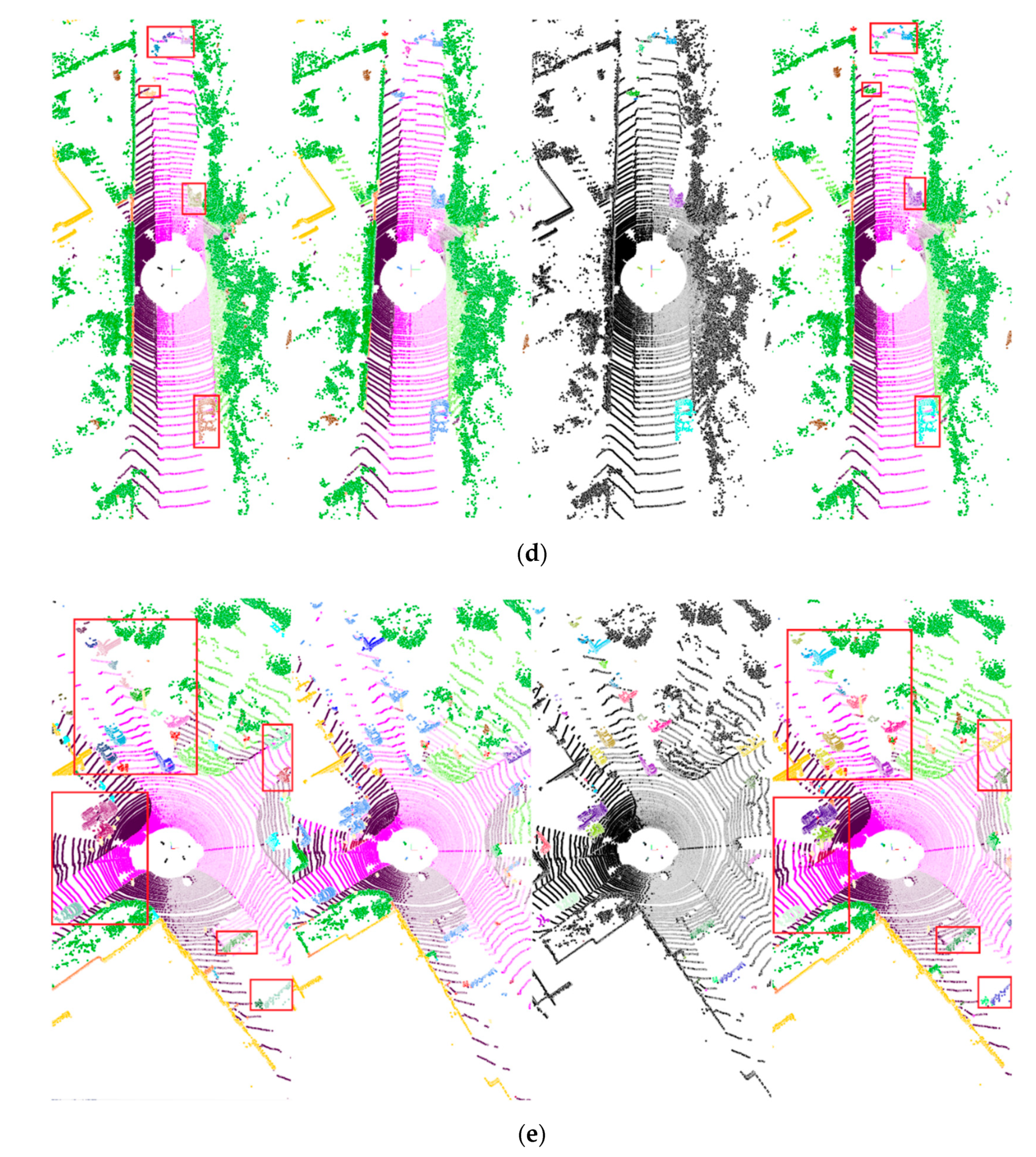
Figure 8.
Visualization of our approach on the validation split of SemanticKITTI—sequence 08. To better distinguish instances, we used red rectangular boxes for identification. From left to right: panoptic ground truth, semantic prediction, instance prediction, panoptic prediction. The colors of the stuff classes are consistent with the legends shown in Figure 1e, and the color of each instance of the thing classes in each subfigure is given randomly. (a) Scan 800. (b) Scan 1600. (c) Scan 2400. (d) Scan 3200. (e) Scan 4000.


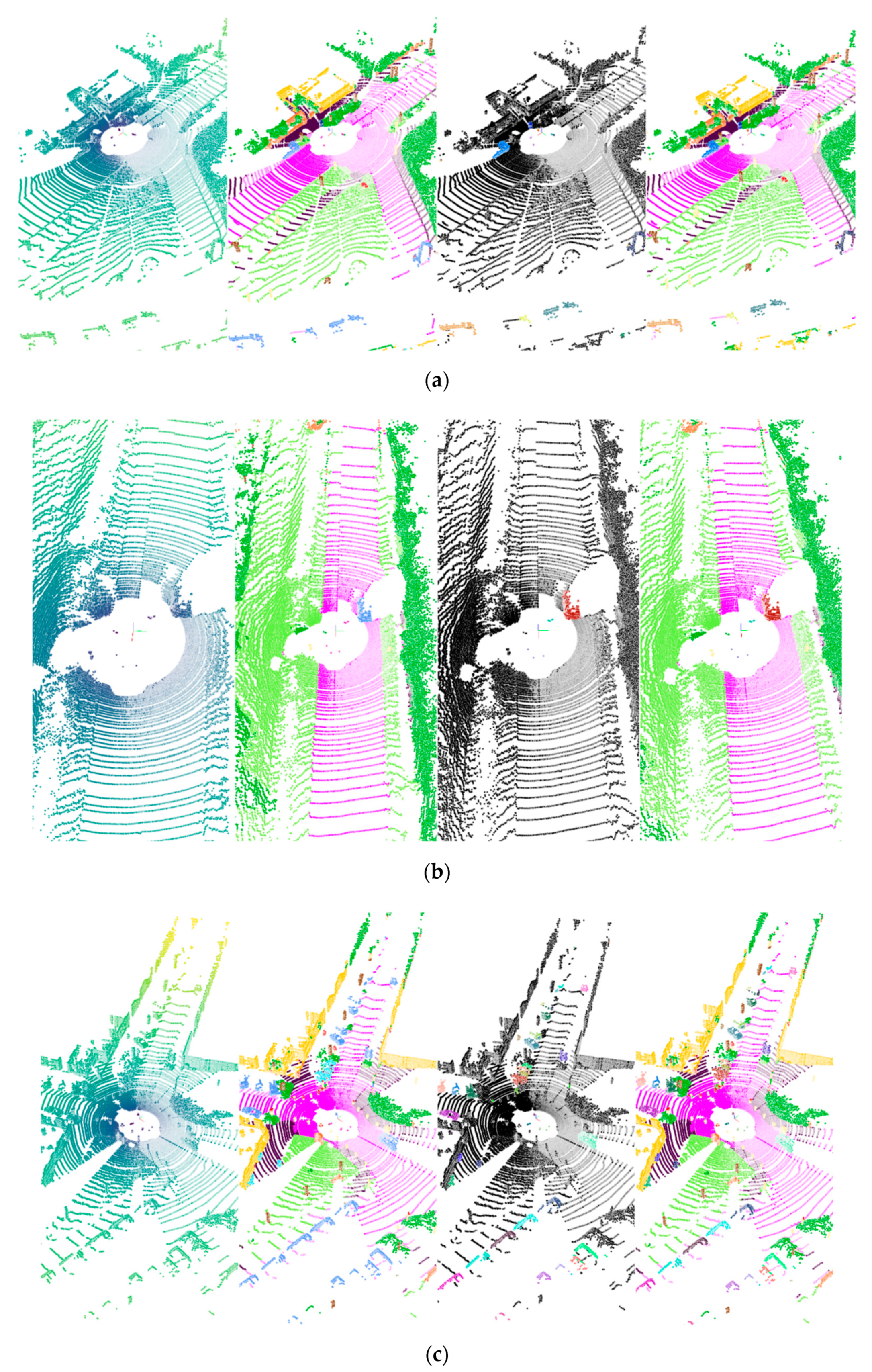
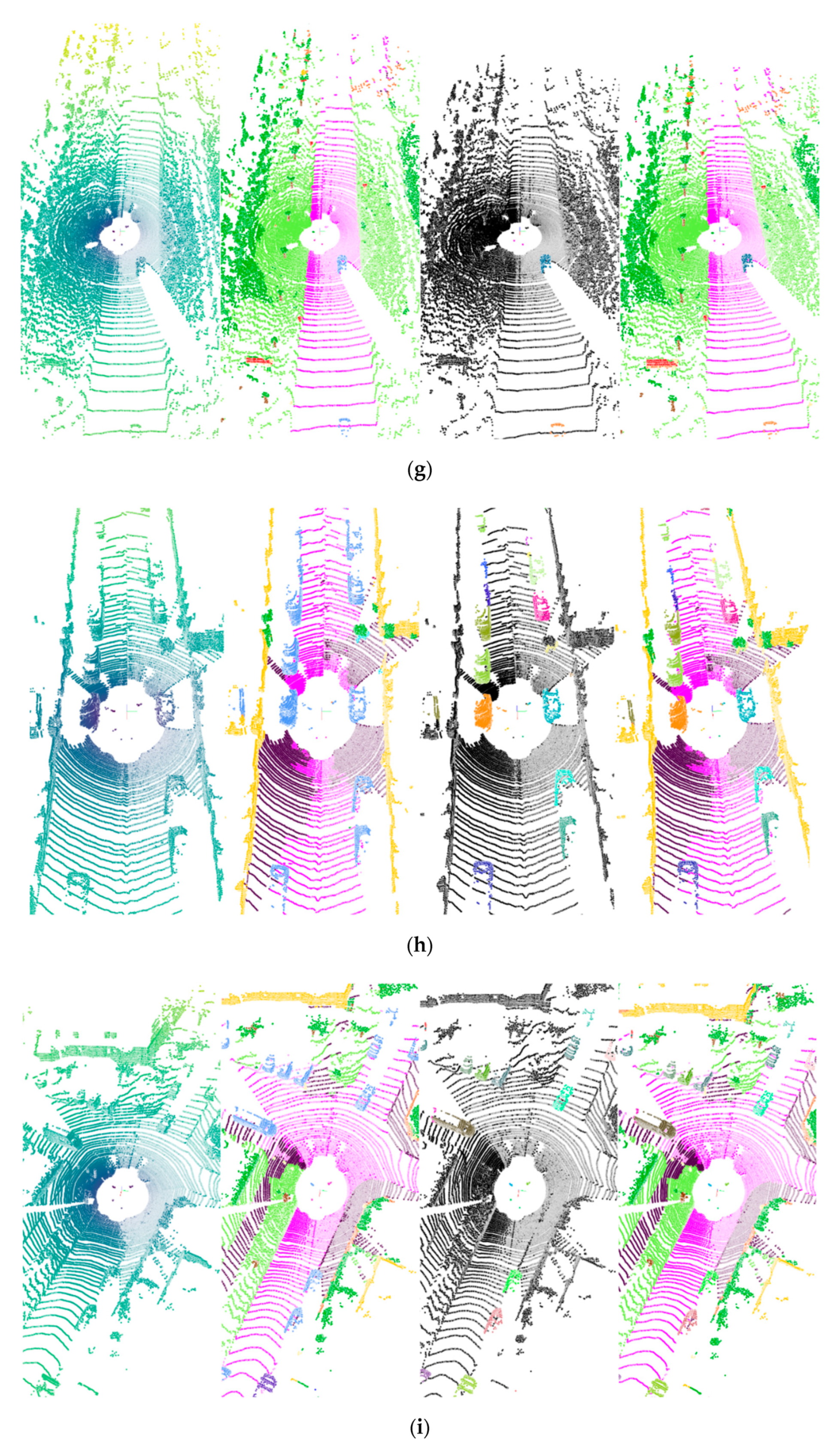
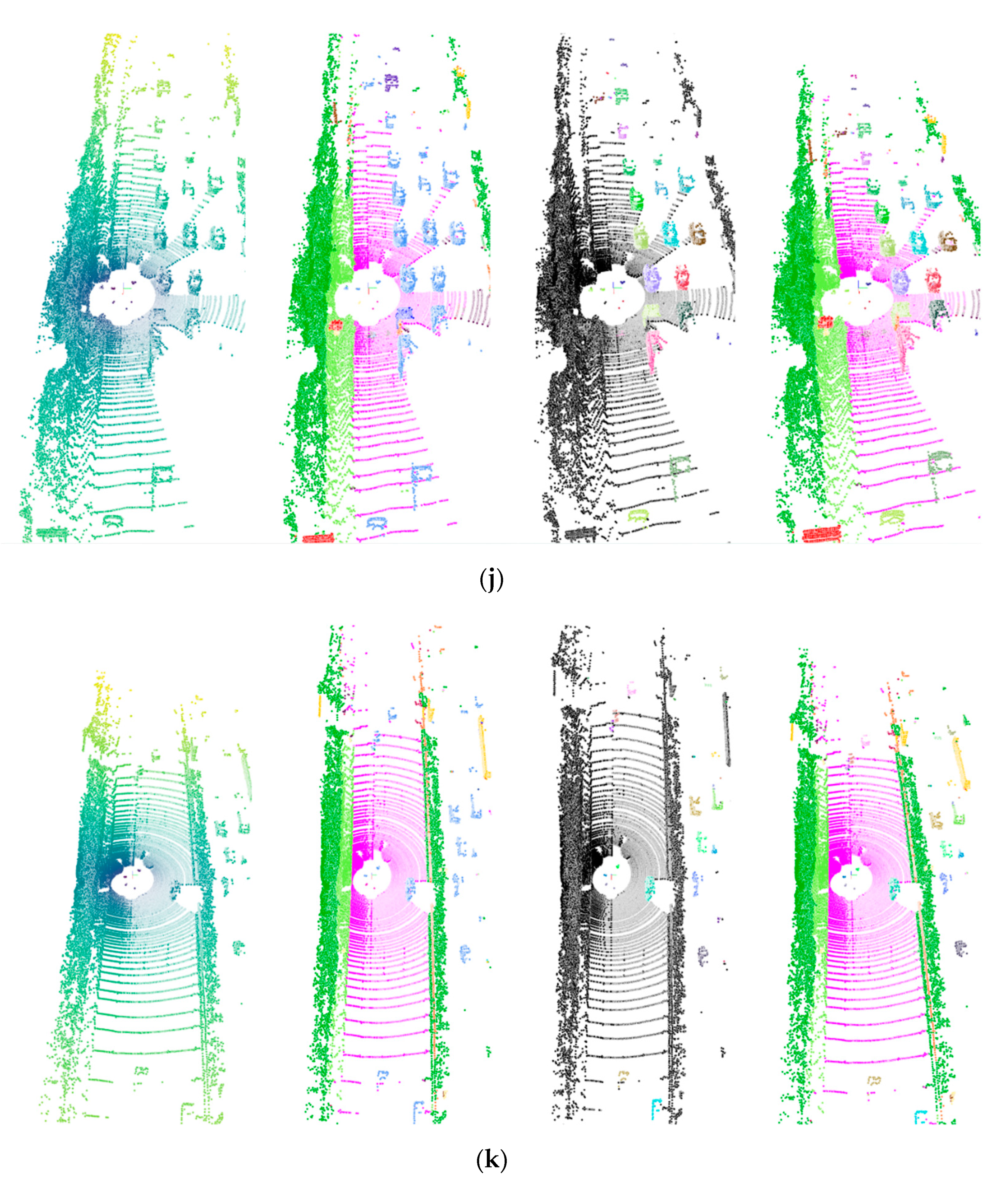
Figure 9.
Visualization of our approach on the test split of SemanticKITTI—sequence 11–21. From left to right: raw scan, semantic prediction, instance prediction, panoptic prediction. The colors of the stuff classes are consistent with the legends shown in Figure 1e, and the color of each instance of the thing classes in each subfigure is given randomly. (a) Sequence 11. (b) Sequence 12. (c) Sequence 13. (d) Sequence 14. (e) Sequence 15. (f) Sequence 16. (g) Sequence 17. (h) Sequence 18. (i) Sequence 19. (j) Sequence 20. (k) Sequence 21.


Figure 10.
Architecture diagram of Polar-Unet3+ and MS-Polar-Unet3+. The difference was that an encoder and decoder were added.
Figure 10.
Architecture diagram of Polar-Unet3+ and MS-Polar-Unet3+. The difference was that an encoder and decoder were added.

Figure 11.
Experimental results of MULLS on the SemanticKITTI dataset. (a) Sequence 00. (b) Sequence 01. (c) Sequence 02. (d) Sequence 03. (e) Sequence 04. (f). Sequence 05. (g) Sequence 06. (h) Sequence 07. (i) Sequence 08. (j) Sequence 09. (k) Sequence 10.
Figure 11.
Experimental results of MULLS on the SemanticKITTI dataset. (a) Sequence 00. (b) Sequence 01. (c) Sequence 02. (d) Sequence 03. (e) Sequence 04. (f). Sequence 05. (g) Sequence 06. (h) Sequence 07. (i) Sequence 08. (j) Sequence 09. (k) Sequence 10.


Table 1.
Statistics on the proportion of various environmental elements in each scan.
| Scan | Car | Bicycle | Motorcycle | Truck | Other-Vehicle | Person | Bicyclist | Motorcyclist | Road | Parking | Sidewalk | Other-Ground | Building | Fence | Vegetation | Trunk | Terrain | Pole | Traffic-Sign | Unlabeled |
|---|---|---|---|---|---|---|---|---|---|---|---|---|---|---|---|---|---|---|---|---|
| 000 | 3.40 | 0 | 0 | 0 | 0 | 0 | 0 | 0.07 | 27.46 | 2.62 | 21.14 | 0 | 14.65 | 0.30 | 21.76 | 0.96 | 2.38 | 0.43 | 0.08 | 4.76 |
| 500 | 10.71 | 0 | 0 | 0 | 0 | 0 | 0 | 0 | 10.95 | 0 | 23.05 | 0 | 26.97 | 3.08 | 22.14 | 0 | 0.05 | 0.13 | 0.05 | 2.87 |
| 1000 | 9.97 | 0 | 0 | 0 | 0 | 0.01 | 0 | 0 | 11.92 | 0 | 19.92 | 0 | 15.71 | 1.39 | 27.90 | 2.95 | 9.09 | 0.03 | 0 | 1.12 |
| 1500 | 12.15 | 0.54 | 1.23 | 0 | 0 | 0 | 0 | 0 | 21.83 | 10.78 | 3.74 | 0 | 38.10 | 0.04 | 7.94 | 2.26 | 0.18 | 0.16 | 0 | 1.05 |
| 2000 | 8.94 | 0 | 0 | 0 | 0 | 0 | 0 | 0 | 12.29 | 0 | 9.77 | 0 | 14.57 | 11.72 | 31.05 | 3.02 | 6.75 | 0.70 | 0.01 | 1.19 |
| 2500 | 7.34 | 0 | 0 | 0 | 0 | 0 | 0 | 0 | 12.08 | 0 | 7.80 | 0 | 27.71 | 4.75 | 13.29 | 0.92 | 22.35 | 0.20 | 0.02 | 3.54 |
| 3000 | 18.13 | 0 | 0 | 0.70 | 2.83 | 0 | 0.13 | 0 | 28.09 | 2.44 | 9.38 | 0 | 6.31 | 0.32 | 20.55 | 1.30 | 5.03 | 0.24 | 0 | 4.55 |
| 3500 | 7.01 | 0 | 0.04 | 0 | 0 | 0 | 0 | 0 | 12.01 | 0.01 | 20.82 | 0 | 24.31 | 4.88 | 25.54 | 0 | 0.14 | 0.31 | 0.05 | 4.88 |
| 4000 | 17.85 | 0 | 0 | 0 | 0 | 0 | 0 | 0 | 14.62 | 0 | 5.85 | 0 | 4.62 | 2.01 | 48.23 | 0.02 | 5.44 | 0.23 | 0 | 1.13 |
| 4500 | 7.55 | 0 | 0 | 0 | 1.02 | 0 | 0 | 0 | 19.74 | 6.54 | 16.19 | 0 | 35.92 | 0.98 | 7.66 | 2.55 | 0 | 0.18 | 0.10 | 1.55 |
| Average | 8.51 | 0.03 | 0.14 | 0.02 | 0.15 | 0.02 | 0.01 | 0 | 16.81 | 1.44 | 14.50 | 0 | 20.91 | 3.66 | 23.74 | 0.88 | 6.29 | 0.34 | 0.04 | 2.52 |
Table 2.
Comparison of LiDAR-based panoptic segmentation performance on the test split of SemanticKITTI. Metrics are provided in [%], and FPS is in [Hz].
Table 2.
Comparison of LiDAR-based panoptic segmentation performance on the test split of SemanticKITTI. Metrics are provided in [%], and FPS is in [Hz].
| Method | PQ | PQ† | RQ | SQ | PQTh | RQTh | SQTh | PQSt | RQSt | SQSt | mIoU | FPS | Runtime | Publication |
|---|---|---|---|---|---|---|---|---|---|---|---|---|---|---|
| RangeNet [20] + PointPillar [41] | 37.1 | 45.9 | 47.0 | 75.9 | 20.2 | 25.2 | 75.2 | 49.3 | 62.8 | 76.5 | 52.4 | 2.4 | 417 ms | IROS/CVPR 2019 |
| KPConv [35] + PointPillar [41] | 44.5 | 52.5 | 54.4 | 80.0 | 32.7 | 38.7 | 81.5 | 53.1 | 65.9 | 79.0 | 58.8 | 1.9 | 526 ms | ICCV/CVPR 2019 |
| SalsaNext [21] + PV-RCNN [42] | 47.6 | 55.3 | 58.6 | 79.5 | 39.1 | 45.9 | 82.3 | 53.7 | 67.9 | 77.5 | 58.9 | — | — | CVPR 2020 |
| MOPT [32] | 43.1 | 50.7 | 53.9 | 78.8 | 28.6 | 35.5 | 80.4 | 53.6 | 67.3 | 77.7 | 52.6 | 6.8 | 147 ms | CVPR 2020 |
| Panoster [43] | 52.7 | 59.9 | 64.1 | 80.7 | 49.9 | 58.8 | 83.3 | 55.1 | 68.2 | 78.8 | 59.9 | — | — | IEEE RAS 2021 |
| DS-Net [8] | 55.9 | 62.5 | 66.7 | 82.3 | 55.1 | 62.8 | 87.2 | 56.5 | 69.5 | 78.7 | 61.6 | 3.4 | 294 ms | CVPR 2021 |
| GP-S3Net [10] | 60.0 | 69.0 | 72.1 | 82.0 | 65.0 | 74.5 | 86.6 | 56.4 | 70.4 | 78.7 | 70.8 | 3.7 | 270 ms | ICCV 2021 |
| 4D-PLS [5] | 50.3 | 57.8 | 61.1 | 81.6 | 45.3 | 53.2 | 84.4 | 54.0 | 66.8 | 79.5 | 61.3 | — | — | CVPR 2021 |
| LPSAD [11] | 38.0 | 47.0 | 48.2 | 76.5 | 25.6 | 31.8 | 76.8 | 47.1 | 60.1 | 76.2 | 50.9 | 11.8 | 85 ms | IROS 2020 |
| Panoptic-PolarNet [9] | 54.1 | 60.7 | 65.0 | 81.4 | 53.3 | 60.6 | 87.2 | 54.8 | 68.1 | 77.2 | 59.5 | 11.6 | 86 ms | CVPR 2021 |
| Ours | 54.6 | 61.5 | 65.5 | 81.7 | 54.0 | 61.9 | 86.7 | 55.1 | 68.2 | 78.1 | 60.6 | 12.7 | 79 ms | — |
Table 3.
Class-wise results on the test split of SemanticKITTI by our approach. Metrics are provided in [%].
Table 3.
Class-wise results on the test split of SemanticKITTI by our approach. Metrics are provided in [%].
| Metrics | Car | Bicycle | Motorcycle | Truck | Other-Vehicle | Person | Bicyclist | Motorcyclist | Road | Parking | Sidewalk | Other-Ground | Building | Fence | Vegetation | Trunk | Terrain | Pole | Traffic-Sign | Mean |
|---|---|---|---|---|---|---|---|---|---|---|---|---|---|---|---|---|---|---|---|---|
| PQ | 91.0 | 43.3 | 46.6 | 28.3 | 33.3 | 62.3 | 70.4 | 56.7 | 88.4 | 29.7 | 59.6 | 3.02 | 82.4 | 48.1 | 79.0 | 56.6 | 42.4 | 53.2 | 63.6 | 54.6 |
| RQ | 97.4 | 60.2 | 55.9 | 32.0 | 37.7 | 73.1 | 77.7 | 61.4 | 96.4 | 39.4 | 75.3 | 5.01 | 88.8 | 63.6 | 95.5 | 75.9 | 57.3 | 72.2 | 80.4 | 65.5 |
| SQ | 93.4 | 71.9 | 83.4 | 88.4 | 88.4 | 85.3 | 90.6 | 92.4 | 91.7 | 75.2 | 79.2 | 60.4 | 92.8 | 75.6 | 82.7 | 74.6 | 74.0 | 73.7 | 79.1 | 81.7 |
| IoU | 95.1 | 49.3 | 42.9 | 37.8 | 38.1 | 60.1 | 63.1 | 29.1 | 90.7 | 57.6 | 73.2 | 18.7 | 90.1 | 61.9 | 84.3 | 69.3 | 67.8 | 60.0 | 62.4 | 60.6 |
Table 4.
Ablation study of the proposed approach with key components (using to represent each component) on the validation split of SemanticKITTI. Metrics are provided in [%].
Table 4.
Ablation study of the proposed approach with key components (using to represent each component) on the validation split of SemanticKITTI. Metrics are provided in [%].
| Architecture | Polar-UNet3+ | Data Fusion | Random Sample | PQ | mIoU |
|---|---|---|---|---|---|
| Baseline: Polar-UNet | -- | -- | -- | 55.4 | 62.8 |
| Proposed | 56.2 | 63.2 | |||
| 57.1 | 62.9 | ||||
| 57.5 | 63.0 |
Table 5.
Ablation study of the proposed approach with different grid sizes on the validation split of SemanticKITTI. Metrics are provided in [%], and FPS is in [Hz].
Table 5.
Ablation study of the proposed approach with different grid sizes on the validation split of SemanticKITTI. Metrics are provided in [%], and FPS is in [Hz].
| Grid Sizes | PQ | mIoU | FPS |
|---|---|---|---|
| 360 × 360 × 32 | 56.4 | 62.6 | 15.1 |
| 480 × 360 × 32 | 57.5 | 63.0 | 12.7 |
| 600 × 360 × 32 | 57.7 | 63.1 | 9.3 |
Table 6.
Comparison of LiDAR-based moving object semantic segmentation performance on the test split of SemanticKITTI. Metrics are provided in [%].
Table 6.
Comparison of LiDAR-based moving object semantic segmentation performance on the test split of SemanticKITTI. Metrics are provided in [%].
| Method | Car | Bicycle | Motorcycle | Truck | Other-Vehicle | Person | Bicyclist | Motorcyclist | Road | Parking | Sidewalk | Other-Ground | Building | Fence | Vegetation | Trunk | Terrain | Pole | Traffic-Sign | Moving Car | Moving Truck | Moving Other-Vehicle | Moving Person | Moving Bicyclist | Moving Motorcyclist | mIoU | |
|---|---|---|---|---|---|---|---|---|---|---|---|---|---|---|---|---|---|---|---|---|---|---|---|---|---|---|---|
| Cylinder3D | Single | 97.1 | 67.6 | 64.0 | 59.0 | 58.6 | 73.9 | 67.9 | 36.0 | 91.4 | 65.1 | 75.5 | 32.3 | 91.0 | 66.5 | 85.4 | 71.8 | 68.5 | 62.6 | 65.6 | — | — | — | — | — | — | 67.8 |
| Multiple | 94.6 | 67.6 | 63.8 | 41.3 | 38.8 | 12.5 | 1.7 | 0.2 | 90.7 | 65.0 | 74.5 | 32.3 | 92.6 | 66.0 | 85.8 | 72.0 | 68.9 | 63.1 | 61.4 | 74.9 | 0 | 0.1 | 65.7 | 68.3 | 11.9 | 52.5 | |
| Ours | 1 + 2 + 0 | 95.4 | 46.9 | 47.3 | 38.0 | 33.9 | 12.8 | 0 | 0 | 91.8 | 68.2 | 75.3 | 6.9 | 90.7 | 64.3 | 84.5 | 70.8 | 66.0 | 62.7 | 62.2 | 81.9 | 5.6 | 3.7 | 55.5 | 66.9 | 27.4 | 50.4 |
| 1 + 2 + 8 | 94.4 | 57.2 | 47.5 | 42.5 | 32.4 | 14.0 | 0 | 0 | 91.3 | 63.2 | 74.4 | 16.5 | 91.2 | 66.6 | 85.7 | 70.9 | 67.0 | 63.6 | 65.4 | 78.5 | 8.1 | 5.9 | 74.3 | 65.9 | 46.3 | 52.9 | |
Table 7.
Comparison of APE for translation part (unit: m).
| Sequences | Raw Scan | Dynamic Moving GT | Dynamic Moving (Our Method) | |||||||||
|---|---|---|---|---|---|---|---|---|---|---|---|---|
| RMSE | Mean | Median | Std. | RMSE | Mean | Median | Std. | RMSE | Mean | Median | Std. | |
| 00 | 1.58 | 1.32 | 1.01 | 0.87 | 1.40 | 1.09 | 0.81 | 0.88 | 1.32 | 1.10 | 0.94 | 0.73 |
| 01 | 5.71 | 5.25 | 5.56 | 2.23 | 2.05 | 1.93 | 1.91 | 0.70 | 2.14 | 2.03 | 1.94 | 0.68 |
| 02 | 11.41 | 10.23 | 8.70 | 5.07 | 5.70 | 4.79 | 4.10 | 3.09 | 5.95 | 5.24 | 4.26 | 2.82 |
| 03 | 0.56 | 0.50 | 0.48 | 0.25 | 0.51 | 0.46 | 0.42 | 0.23 | 0.54 | 0.49 | 0.46 | 0.23 |
| 04 | 0.45 | 0.41 | 0.41 | 0.18 | 0.40 | 0.37 | 0.35 | 0.15 | 0.44 | 0.41 | 0.38 | 0.16 |
| 05 | 0.80 | 0.67 | 0.53 | 0.45 | 0.60 | 0.48 | 0.37 | 0.36 | 0.71 | 0.60 | 0.51 | 0.37 |
| 06 | 0.64 | 0.40 | 0.25 | 0.50 | 0.38 | 0.29 | 0.23 | 0.24 | 0.49 | 0.34 | 0.26 | 0.35 |
| 07 | 0.89 | 0.78 | 0.63 | 0.44 | 0.50 | 0.44 | 0.43 | 0.23 | 0.54 | 0.48 | 0.50 | 0.25 |
| 08 | 2.32 | 1.99 | 1.85 | 1.19 | 2.12 | 1.78 | 1.58 | 1.16 | 2.16 | 1.84 | 1.62 | 1.13 |
| 09 | 2.10 | 1.68 | 1.38 | 1.26 | 1.95 | 1.58 | 1.14 | 1.14 | 2.03 | 1.62 | 1.15 | 1.22 |
| 10 | 1.22 | 1.17 | 1.13 | 0.33 | 1.20 | 1.15 | 1.12 | 0.35 | 1.17 | 1.12 | 1.07 | 0.33 |
Publisher’s Note: MDPI stays neutral with regard to jurisdictional claims in published maps and institutional affiliations. |
© 2022 by the authors. Licensee MDPI, Basel, Switzerland. This article is an open access article distributed under the terms and conditions of the Creative Commons Attribution (CC BY) license (https://creativecommons.org/licenses/by/4.0/).
Share and Cite
MDPI and ACS Style
Wang, W.; You, X.; Yang, J.; Su, M.; Zhang, L.; Yang, Z.; Kuang, Y. LiDAR-Based Real-Time Panoptic Segmentation via Spatiotemporal Sequential Data Fusion. Remote Sens. 2022, 14, 1775. https://doi.org/10.3390/rs14081775
AMA Style
Wang W, You X, Yang J, Su M, Zhang L, Yang Z, Kuang Y. LiDAR-Based Real-Time Panoptic Segmentation via Spatiotemporal Sequential Data Fusion. Remote Sensing. 2022; 14(8):1775. https://doi.org/10.3390/rs14081775
Chicago/Turabian StyleWang, Weiqi, Xiong You, Jian Yang, Mingzhan Su, Lantian Zhang, Zhenkai Yang, and Yingcai Kuang. 2022. "LiDAR-Based Real-Time Panoptic Segmentation via Spatiotemporal Sequential Data Fusion" Remote Sensing 14, no. 8: 1775. https://doi.org/10.3390/rs14081775
Note that from the first issue of 2016, this journal uses article numbers instead of page numbers. See further details here.