Towards Predicting the Measurement Noise Covariance with a Transformer and Residual Denoising Autoencoder for GNSS/INS Tightly-Coupled Integrated Navigation

Abstract

The tightly coupled navigation system is commonly used in UAV products and land vehicles. It adopts the Kalman filter to combine raw satellite observations, including the pseudorange, pseudorange rate and Doppler frequency, with the inertial measurements to achieve high navigational accuracy in GNSS-challenged environments. The accurate estimation of measurement noise covariance can ensure the quick convergence of the Kalman filter and the accuracy of the navigation results. Existing tightly coupled integrated navigation systems employ either constant noise covariance or simple noise covariance updating methods, which cannot accurately reflect the dynamic measurement noises. In this article, we propose an adaptive measurement noise estimation algorithm using a transformer and residual denoising autoencoder (RDAE), which can dynamically estimate the covariance of measurement noise. The residual module is used to solve the gradient degradation problem. The DAE is adopted to learn the essential characteristics from the noisy ephemeris data. By introducing the attention mechanism, the transformer can effectively learn the time and space dependency of long-term ephemeris data, and thus dynamically adjusts the noise covariance with the predicted factors. Extensive experimental results demonstrate that our method can achieve sub-meter positioning accuracy in the outdoor open environment. In a GNSS-degraded environment, our proposed method can still obtain about 3 m positioning accuracy. Another test on a new dataset also confirms that our proposed method has reasonable robustness and adaptability.

1. Introduction

In the GNSS/INS integrated system, INS is an autonomous navigation system that relies on airborne equipment to complete navigation tasks autonomously [1,2,3]. However, the accumulation of position errors over time leads to poor accuracy. GNSS can obtain stable solutions in an open-sky environment, but its accuracy is severely reduced in the urban canyon with high-rise buildings, inside tunnels and under dense tree canopies [4]. Therefore, combining the above two systems together can effectively leverage their respective advantages to form a navigation system with long-term stability, self-restraint, and high-frequency output [3,4,5,6]. Regarding the integration of GNSS/INS, the most common mode is the loosely coupled (LC) mode [7]. The implementation of LC mode is relatively simple, but in the case of GNSS it must be receiving more than four satellites. However, the tightly coupled (TC) method is to directly fuse the GNSS raw output observations with the INS output, so the tightly coupled mode can still provide GNSS signal updates when fewer than four satellites are received [8].

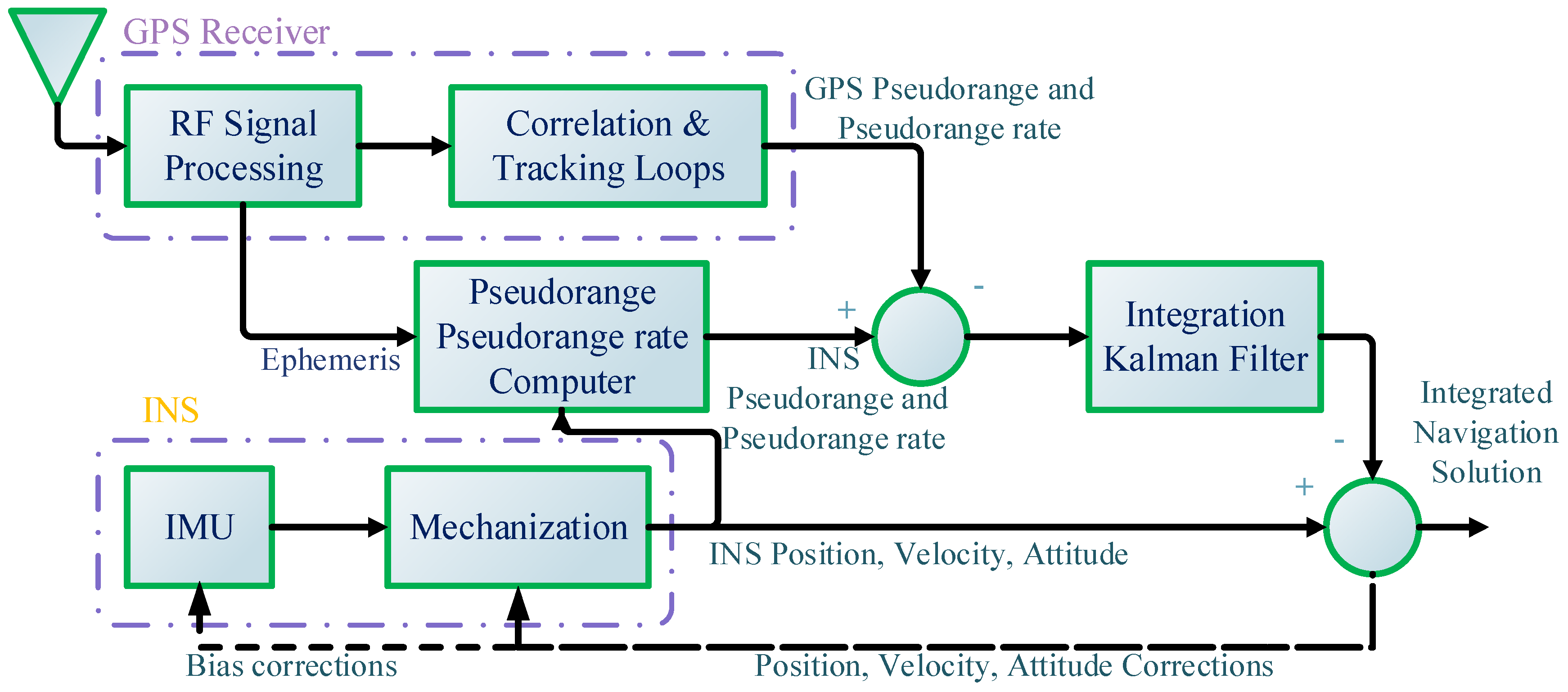
The TC integrated system can obtain better positioning accuracy in harsh environments. At this time, satellite signals may be blocked, making the statistical characteristics of measurement noise uncertain and time-varying. Inaccurate estimation of measurement noise covariance causes filter divergence [9]. A TC integration system uses the GNSS raw observation data (pseudorange and pseudorange rate measurements) as a reference to evaluate and correct the INS error [10]. For the measurement noise covariance in a tightly coupled integrated navigation system, traditional methods generally assume that it is a fixed a priori constant value, but it cannot truly represent the actual statistical characteristics of the measurement noise during actual operation. In actual navigation system applications, in order to be able to deal with the instability of the measurement noise covariance matrix [11], the adaptive Kalman filter (AKF) that can estimate R online should be used to ensure the positioning accuracy and continuity of the navigation results [12].

In recent years, deep learning domain knowledge has been widely used in natural language processing and computer vision [13]. These methods discover complex structures through specific backpropagation and error correction mechanisms to instruct the machine how to change its internal parameters for learning features. Because a neural network has an ability to learn data relationships, for this article a neural network algorithm was designed in the TC integrated system. The algorithm can automatically learn the measurement noise parameters online and make adaptive adjustments according to the actual environment, so that the Kalman filter can perform accurate position estimation.

Conventionally, due to the inaccurate statistical characteristics of noise, the model cannot reflect the real physical process, so the observed values do not correspond to the model, which in turn leads to filter divergence [14]. In practical application scenarios, it is inaccurate to assume that the noise is fixed. Therefore, adaptively adjusting the statistical characteristics of noise for different actual environments is more in line with the navigation process and improves the positioning performance in challenging environments.

For solving the problem of noise covariance estimation in the GNSS/INS integrated system, various adaptive adjustment methods have been developed in different scenarios [15]. Cho and Choi combined Sigma-point KF (SPKF) with a receding-horizon strategy to propose a new filtering scheme that is beneficial for reducing initial estimation error and temporal unknown bias [16]. Gao et al. [17] proposed a strategy of seam tracking monitoring, in which the Sage–Husa AKF is given to estimate the statistical characteristics of noise, and the filter parameters are adjusted to achieve an adaptive ability in the case of noise changes. He et al. [18] proposed a method to estimate the covariance matrix of measurement noise using a simplified Sage–Husa filter. Meng et al. [15] presented an adaptive unscented Kalman filter (UKF) with a noise statistic estimator to make up for some of the shortcomings of the standard UKF.

Furthermore, covariance matching technology uses innovative covariance or residual covariance to reasonably estimate the covariance of the process noise and measurement noise at each sampling moment [19]. When the statistical characteristics of noise need to be estimated, using the IAE method to estimate the covariance reduces the navigation accuracy, and even causes a risk of filtering divergence [20]. In response to this problem, Zhang et al. [21] proposed an INS/GNSS integrated navigation system adaptive estimation (RMAE) method based on redundant measurements, which uses the INS solution as redundant measurements to estimate the measurement noise covariance matrix. Due to the advantages of this aspect, in order to solve the coupling problem of estimating the measurement value and the process noise covariance at the same time, Ge et al. [22] proposed a scheme combining the RMAE method with the estimation algorithm of process noise covariance. To improve the position accuracy and reliability, Ge et al. [23] proposed a strategy for the mitigation of GNSS measurement disturbances in which the time-varying covariance of measurement noise is estimated by RMAE and Burg methods according to the statistical characteristics of the difference sequences. Sun et al. [24] proposed a pseudorange error prediction method based on an ensemble bagged regression tree that updates the measurement noise covariance for tightly coupled GNSS/IMU navigation systems in urban areas. Ding et al. [25] combined Bayesian inference methods with unscented Kalman filters to propose a new algorithm for estimating aerodynamic parameters and noise in aircraft dynamical systems. Bao et al. [26] established an adaptive maneuvering target-tracking method using the interactive multiple method (IMM) for maneuver identification, and, at the same time, introduced the Sage–Husa adaptive filtering algorithm to estimate the measurement noise covariance in real time.

Due to the powerful data representation capabilities of neural networks in computer vision and natural language processing, there have been some methods combining neural networks with KF to improve the positioning accuracy of INS/GNSS integrated navigation systems. Haarnoja et al. [27] designed a neural network suitable for state estimation by using covariance matrices to convey the expected degree of uncertainty in observations. Liu et al. [28] introduced deep inference for covariance estimation (DICE) to predict the covariance of a sensor measurement from raw sensor data. The model restricts covariance predictions to positive definite values using a deep convolutional neural network to learn a noise model of sensor measurements. Coskun et al. [29] proposed the LSTM Kalman filter (LSTM-KF), a new architecture which can learn the motion model and all noise parameters of the Kalman filter, thus allowing us to train our models with less data successfully. In the LC integrated navigation system, Gao et al. [30] introduced reinforcement learning to estimate the process noise covariance adaptively. The algorithm takes the navigation system as the environment, takes the negative value of the positioning error as the reward and uses the deep deterministic policy as the gradient to obtain the optimal estimation. Wu et al. [31] proposed an algorithm based on a multi-task learning model, which can estimate the processing noise covariance and measurement noise covariance of a Kalman filter simultaneously.

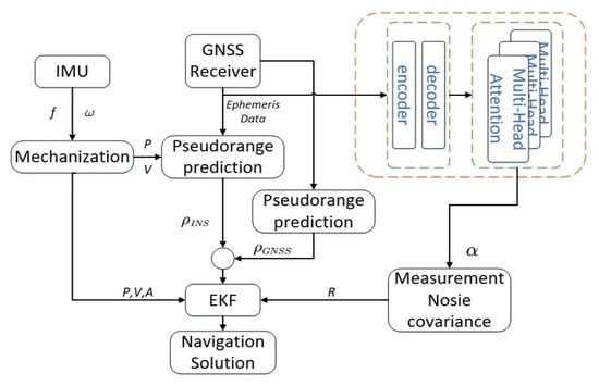
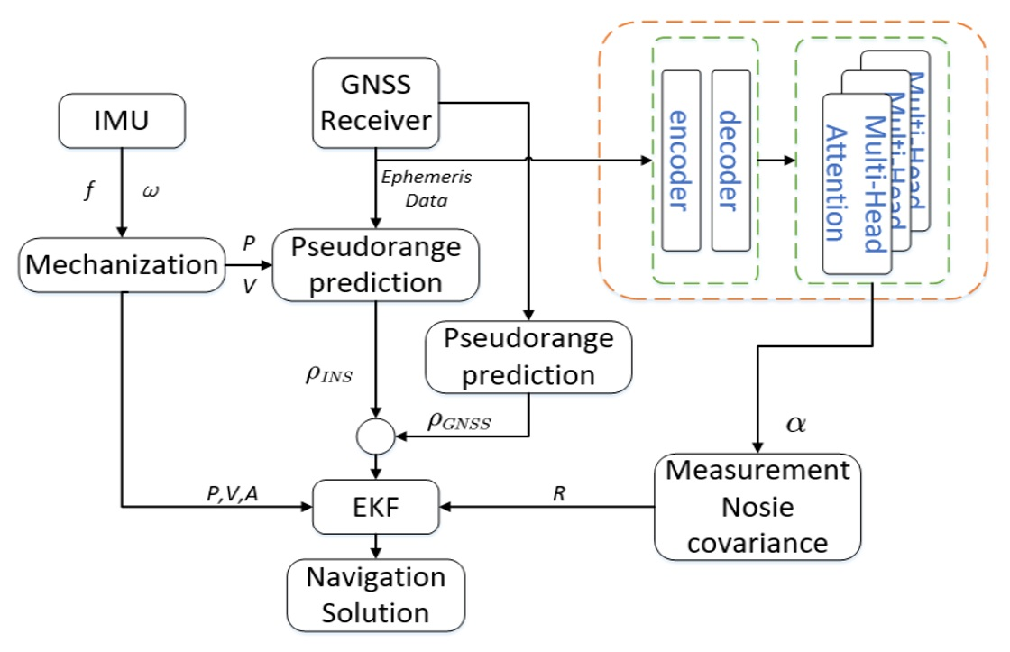
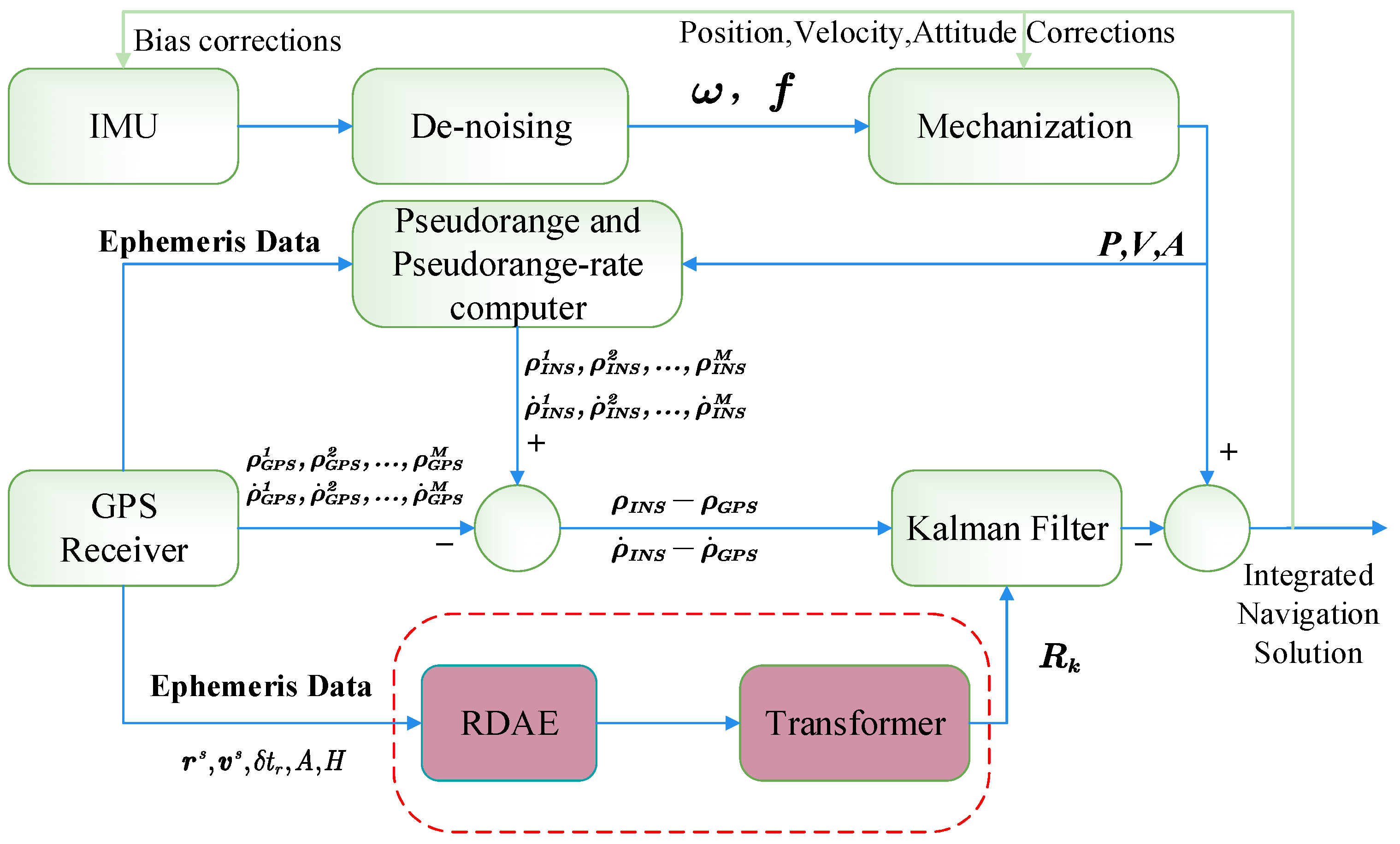
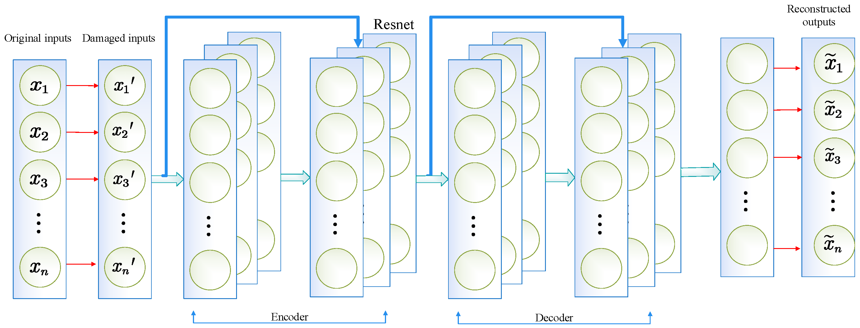
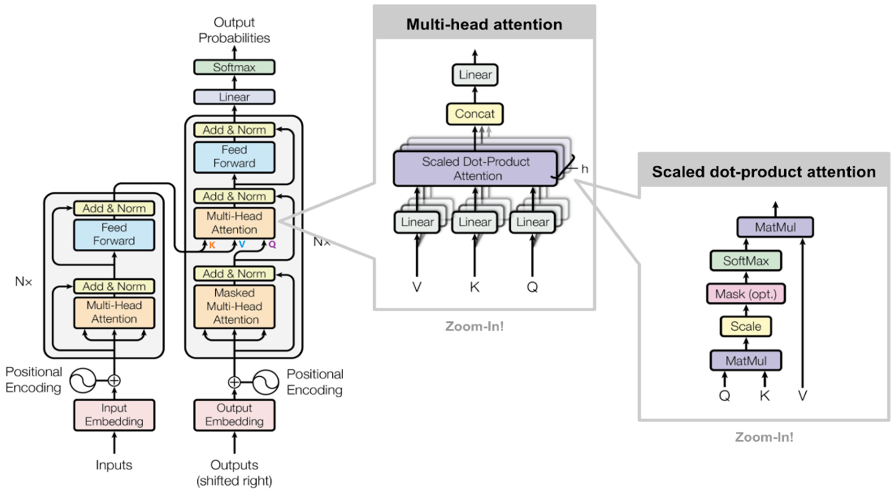
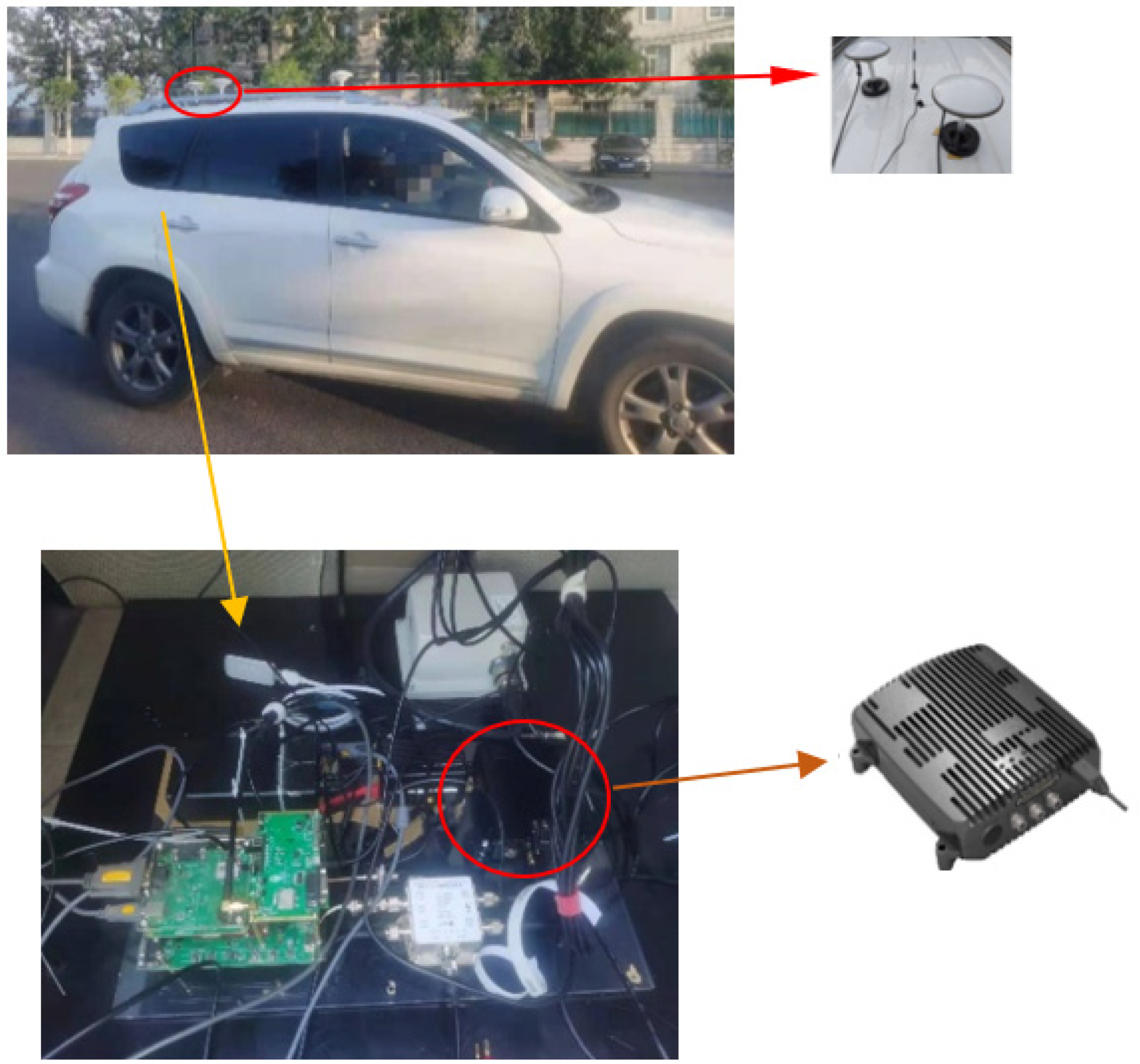
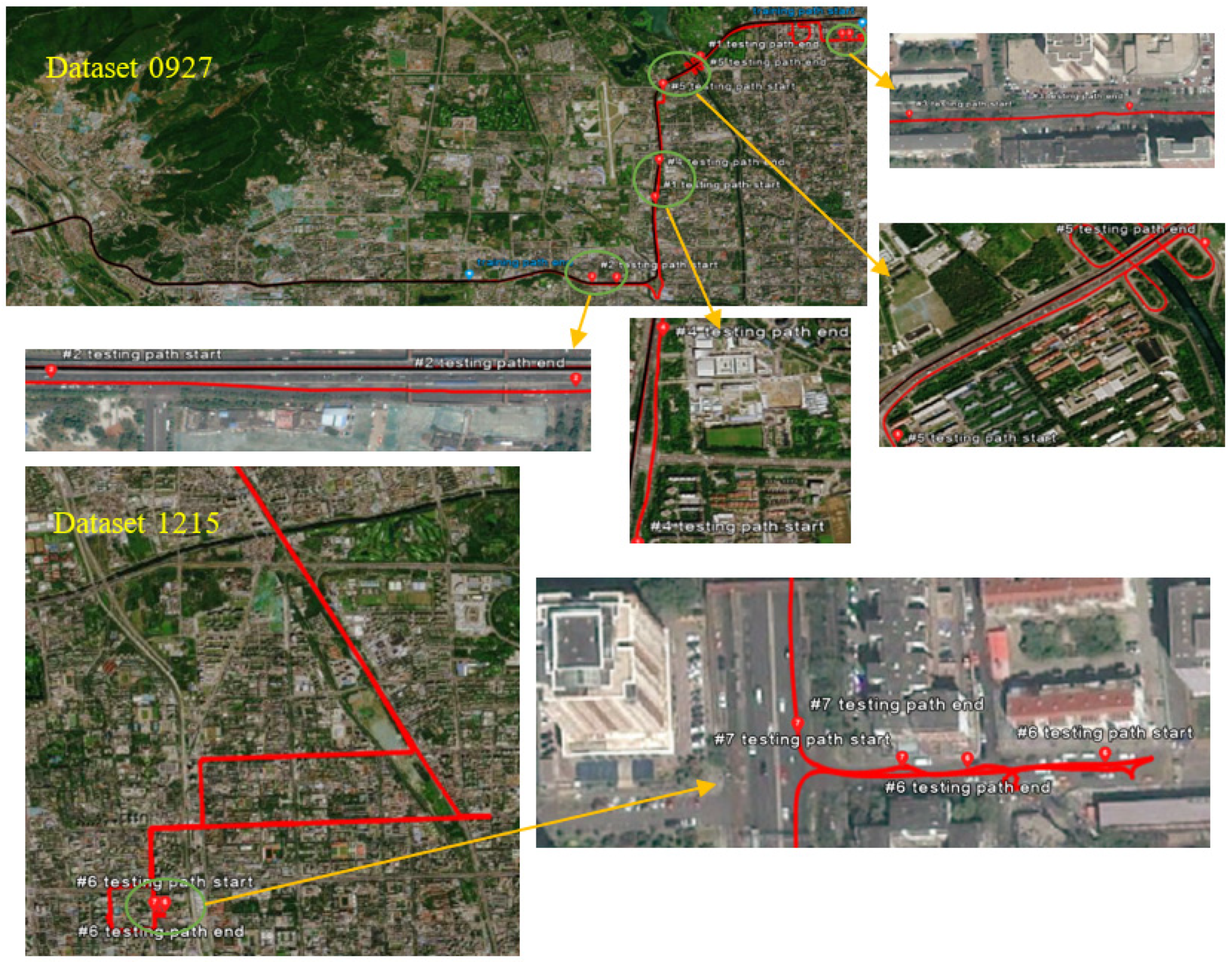
We propose a transformer-based noise covariance prediction model, which exploits an attention mechanism to learn the uncertainty of current raw satellite observations, and combines it with a Kalman filter to adaptively adjust the measurement noise covariance. Before the data enters the transformer network model, we use the residual denoising autoencoder (RDAE) to filter the original data. This method can make the model obtain better generalization ability, and make the task of adaptive adjustment of measurement noise covariance better. We conducted extensive experiments on practical road test data to evaluate our proposed navigation algorithm. Experimental results indicate that our proposed method is superior to the traditional algorithm of adjusting the covariance matrix of measurement noise, and obtains the best performance in comparison with other networks.

The remainder of this paper is organized as follows: Section 2 briefly introduces the INS/GNSS tightly coupled integrated system and our proposed algorithm; Section 3 demonstrates and presents an analysis of the algorithm based on actual road tests; Section 4 discusses the experimental results; and Section 5 presents the final conclusion.

2. Materials and Methods

In this study, the tightly coupled navigation system was considered to have a higher performance than the loosely coupled navigation system. We first describe the standard tightly coupled integrated system [32], the block diagram of which is shown in Figure 1. As shown in Figure 1, the difference between pseudorange and pseudorange rate measurements from the GNSS and corresponding INS prediction values are fed into the KF to estimate the INS error. Then, the output result of the INS is corrected according to the correlation error to obtain the final navigation and positioning result.

2.1. Tightly Coupled Integration Dynamic Model

The state transition equation of the inertial navigation system is as follows:

$$\delta \dot{X_I}=F_I{X}_I+G_I{\omega }_I$$

(1)

where the state vector $\delta \dot{X}=\left[\delta r,\delta v,\phi ,b_a,b_g\right]$ includes the position error

The term $F_I$ is the dynamic coefficient matrix of the INS error with the following formula:

$$F_I=\left[\begin{array}{cc}\begin{array}{ccc}{0}_{3\times 3}& F_r& 0_{3\times 3}\\ 0_{3\times 3}& 0_{3\times 3}& F_v\\ 0_{3\times 3}& F_{\epsilon }& 0_{3\times 3}\end{array}& \begin{array}{cc}{0}_{3\times 3}& 0_{3\times 3}\\ 0_{3\times 3}& R_b^l\\ R_b^l& 0_{3\times 3}\end{array}\\ \begin{array}{ccc}{0}_{3\times 3}& 0_{3\times 3}& 0_{3\times 3}\\ 0_{3\times 3}& 0_{3\times 3}& 0_{3\times 3}\end{array}& \begin{array}{cc}{F}_{\omega }& 0_{3\times 3}\\ 0_{3\times 3}& F_f\end{array}\end{array}\right]$$

(2)

where F_r, F_v, F_ε are the correlation matrices of the position, velocity and attitude error equations, respectively; the formula is as follows:

$$F_r=\left[\begin{array}{ccc}0& \frac{1}{\left(R_M+h\right)}& 0\\ \frac{1}{\left(R_M+h\right)\cos \phi }& 0& 0\\ 0& 0& 1\end{array}\right], F_v=\left[\begin{array}{ccc}0& f_u& -f_n\\ -f_u& 0& f_e\\ f_n& -f_e& 0\end{array}\right], F_r=\left[\begin{array}{ccc}0& \frac{1}{\left(R_M+h\right)}& 0\\ \frac{-1}{\left(R_N+h\right)}& 0& 0\\ \frac{-\tan \phi }{\left(R_N+h\right)}& 0& 1\end{array}\right]$$

(3)

$R_b^l$ is the rotation matrix from the b-frame to the l-frame; $F_{\omega }$ $F_f$ are the correlation matrices of the error models of the gyroscope and accelerometer, which conform to a first-order Markov process.

The state transition equation of the GNSS is as follows:

$$\delta \dot{X_G}=F_G{X}_G+G_G{\omega }_G$$

(4)

where the state vector of the GNSS model $\delta X_G=\left[\begin{array}{cc}\Delta t_r& \Delta {\dot{t}}_r\end{array}\right]$ includes the receiver clock error $\Delta t_r$ and clock drift $\Delta {\dot{t}}_r$. The coefficient matrix of GNSS error is

$$F_G=\left[\begin{array}{cc}0& 1\\ 0& 0\end{array}\right]$$

(5)

The error models of the INS and GNSS are combined as follows:

$$\delta \dot{X}=F\delta X+G\omega$$

(6)

$$\left[\begin{array}{c}\delta \dot{X_I}\\ \delta \dot{X_G}\end{array}\right]=\left[\begin{array}{cc}{F}_I& 0\\ 0& F_G\end{array}\right]\left[\begin{array}{c}\delta X_I\\ \delta X_G\end{array}\right]+\left[\begin{array}{c}{G}_I\\ G_G\end{array}\right]\omega$$

(7)

2.2. Tightly Coupled Integration Measurement Model

The error model of measurement is expressed as

$$\delta Z_k=H_k\delta X_k+{\epsilon }_k$$

(8)

where $H_k$ is the measurement matrix, which defines the change rule of the observation vector with the state, and the formula is as follows:

$$H_k=\begin{array}{cc}\begin{array}{ccc}{H}_{M\times 3}^{\rho }& 0_{M\times 3}& 0_{M\times 9}\\ 0_{M\times 3}& H_{M\times 3}^{\dot{\rho }}& 0_{M\times 9}\end{array}& \begin{array}{cc}-1_{M\times 1}& 0_{M\times 1}\\ 0_{M\times 1}& -1_{M\times 1}\end{array}\end{array}$$

$H_{M\times 3}^{\rho }$ and $H_{M\times 3}^{\dot{\rho }}$ are converted from unit line of sight vectors.

The measurement information is composed of the difference between the observed values of the pseudorange and pseudorange rate obtained by the GNSS and the predicted value calculated by the INS.

$$\delta Z=\left[\begin{array}{c}\delta Z_{\rho }\\ \delta Z_{\dot{\rho }}\end{array}\right]=\left[\begin{array}{c}{\rho }_{INS}-{\rho }_{GPS}\\ {\dot{\rho }}_{INS}-{\dot{\rho }}_{GPS}\end{array}\right]$$

(9)

2.2.1. Pseudorange Measurements

Since we need to propagate the error state in the KF process, the pseudorange is written in the following format:

$$\delta Z_{\rho }={\rho }_{INS}-{\rho }_{GPS}$$

(10)

The pseudorange obtained by the GNSS receiver is modeled [33] as the following formula:

$${\rho }_{GPS}^m=r^m+c\Delta t_r-c\Delta t_s+c{I}^m+c{T}^m+{\epsilon }_{\rho }^m$$

(11)

where $r^m$ is the geometric distance, $\Delta t_r$ is the receiver’s clock offset, $\Delta t_s$ is the satellite’s clock offset, $c$ is the speed of light, $I^m$ is the ionospheric delay, $T^m$ is the tropospheric delay and ${\epsilon }_{\rho }^m$ are other errors.

The pseudorange calculated from the inertial navigation output and satellite ephemeris information is as follows [34]:

$${\rho }_{INS}^m=\sqrt{{\left(x_{INS}-x^m\right)}^2+{\left(y_{INS}-y^m\right)}^2+{\left(z_{INS}-z^m\right)}^2}$$

(12)

where $X_{INS}={\left[x_{INS},y_{INS},z_{INS}\right]}^T$ is the output of INS and $X^m={\left[x^m,y^m,z^m\right]}^T$ is the $m^{th}$ satellite’s position.

2.2.2. Pseudorange Rate Measurements

The formula for the measurement value of the pseudorange rate is as follows:

$$\delta Z_{\dot{\rho }}={\dot{\rho }}_{INS}-{\dot{\rho }}_{GPS}$$

(13)

The formula for calculating the Doppler shift is as follows:

$$D^m=\frac{\left[\left(v^m-v\right)·I^m\right]L}{c}$$

(14)

where $v^m={\left[v_x^m,v_y^m,v_z^m\right]}^T$ is the velocity of the satellite, $v={\left[v_x,v_y,v_z\right]}^T$ is the true receiver velocity, $L$ is the satellite’s transmission frequency, $I^m$ is the line of sight unit vector from the satellite to the GNSS receiver.

Given the Doppler value, the pseudorange rate can be computed as

$${\dot{\rho }}_{GPS}^m=-\frac{D^{m}c}{L}$$

(15)

The formula for calculating an estimate of the pseudorange rate by the INS is as follows:

$${\dot{\rho }}_{INS}^m=I_x^m\left(v_{x,I}-v_x^m\right)+I_y^m\left(v_{y,I}-v_y^m\right)+I_z^m\left(v_{z,I}-v_z^m\right)$$

(16)

where $v_{x,I}, v_{y,I}, v_{z,I}$ are the receiver’s velocities in the e-frame estimated by the INS.

2.3. Navigation Fusion with EKF

The data output results of the INS and GNSS systems can be fused by EKF. The solution of EKF is a iterative procedure with time update step given by [35] as follows

$$\{\begin{array}{c}{x}_k^{-}={\mathsf{\Phi }}_{k,k-1}{x}_{k-1}^{+}\\ P_k^{-}={\mathsf{\Phi }}_{k,k-1}{P}_{k-1}^{+}{\mathsf{\Phi }}_{k,k-1}^T+Q_{k-1}\end{array}$$

(17)

where $x_{k-1}^{+}$ is the state estimation at time $k-1$ and $P_{k-1}^{+}$ is the estimation covariance. $x_k^{-}$ and $P_k^{-}$ denote the state prediction value and prediction covariance value at time $k$. ${\mathsf{\Phi }}_{k,k-1}$ is the state transition matrix. $Q_{k-1}$ is the process noise covariance matrix.

The measurement updating step is provided as

$$\{\begin{array}{c}{K}_k=P_k^{-}{H}_k^T{\left(H_k{P}_k^{-}{H}_k^T+R_k\right)}^{-1}\\ x_k^{+}=x_k^{-}+K_k\left(\delta Z_k-H_k{x}_k^{-}\right)\\ P_k^{+}=\left(I-K_k{H}_k\right)P_k^{-}\end{array}$$

(18)

where $\delta Z_k$ denotes the measurement vector and $H_k$ is the measurement matrix. $K_k$ denotes the Kalman gain and $R_k$ is the noise covariance matrix of measurement.

2.4. Proposed Methodology

In this section, we introduce the framework of the algorithm, which is based on a tightly coupled integration framework, by applying a neural network approach to adjust the measurement covariance matrix R adaptively, as Figure 2 shows. First, for the deep residual denoising auto-encoder, the unsupervised method is used for training, and the signal reconstruction strategy is used to filter the sensor measurement noise; we subsequently use it to extract valuable features for later tasks. Then, we utilize a transformer network to accurately adjust the covariance matrix of the measurement noise in the tightly coupled system adaptively, and our proposed RT algorithm obtains high-precision and high-continuity positioning in challenging and complex environments. Next, we present the details of these modules.

2.4.1. Residual Denoising Auto-Encoder

Considering that the raw data from satellite ephemeris inevitably contain various noises, we use the proposed RDAE neural network for feature extraction, which fundamentally combines the advantages of Resnet and AE, and eliminates the relevant noise in the original sensor data through the method of signal reconstruction. Firstly, the data feature loss phenomenon is simulated by randomly removing features from the original input matrix using some probability distribution. The network uses this missing data to calculate and iterate the error between the refined data and the original. In this way, the network learns the corrupted data. There are two reasons why this corrupted data is very significant: For one, the weight noise trained on corrupted data is relatively small by comparison with non-corrupted data training. Second, the corrupted data, to some extent, reduces the gap between the training data and the test data. The robustness of the weight trained in this way is improved [36]. As illustrated by Figure 3, the encoder and decoder of RDAE contains Resnet rather than the fully connected layers.

The composition of the raw input data at time $t$ is $x\left(t\right)=\left\{r^s\left(t\right),v^s\left(t\right),\Delta t_r\left(t\right),A\left(t\right),H\left(t\right)\right\}$ (satellite position, satellite speed, receiver clock bias, azimuth, elevation).

Given the noisy training samples, $X={\left\{x\left(t\right)\right\}}_{t=1}^T$ and the corresponding corrupted samples are $\tilde{X}={\left\{\tilde{x}\left(t\right)\right\}}_{t=1}^T$ (i.e., dropout), where $T$ is the final time of the training data.

The network is trained by minimizing the error between the training data and the output data with the following formula:

$$L\left(X,\tilde{X}\right)=\frac{1}{2}\Vert X-\tilde{X}\Vert {}_2^2$$

(19)

Next, we perform supervised fine-tuning of the network, then perform this “denoising” process, and the final feature map of the encoder is applied to the following network tasks.

2.4.2. Measurement Noise Estimation Based on Transformer

In this section, we propose a new algorithm based on a transformer, which can adaptively estimate the measurement noise covariance of GNSS/INS in tightly coupled integrated navigation.

When RTK-fixed solutions are available from GNSS signals, as shown in Figure 2, the algorithm we propose is suitable for the training mode. Firstly, the covariance matrix of measurement noise is initialized, and then the network takes $r^s,v^s,\Delta t_r,A,H$ as the inputs of the RT. A Kalman filter is used to optimize the inertial navigation error estimation by integrating the inertial navigation output and GNSS measurement data. The inertial navigation output is corrected using the optimized inertial navigation error estimation results to obtain the estimation results of positioning, velocity and attitude. Regarding the parameter selection of the transformer, the data dimension of the encoder and decoder is 32, which corresponds to the number of GNSSs at the same time; the number of attention heads is 8; the number of encoder and decoder layers is 6; the linear layer dimension is 2048. The input data of the network are the position, velocity, clock error, azimuth and elevation of each satellite at each moment. We believe that the observation noise level of the satellite at this moment can be deduced by analyzing the characteristics of these data. In addition, the feature is extracted by the attention analysis mechanism of the data. The length of the vector is 32, which corresponds to the respective data of 32 satellites at the same time. The output sequence of the network has a length of 2 and a dimension of 32, representing the observed noise levels of the pseudorange and pseudorange rate of the 32 satellites, respectively. The network output is used to adjust the R matrix, and the subsequent process of the Kalman filter is also incorporated into the network gradient propagation chain; that is, the other intermediate quantities of the Kalman filter are passed into the network as parameters. Finally, the final position is used for loss calculation and backpropagation.

When the car is running in harsh environments, such as viaducts, tree-lined roads or urban canyons, the signal received by the GNSS is relatively weak and the noise is relatively large. At this time, the accurate measurement of the covariance estimation matrix R has a great influence on the results of GNSS/INS integrated navigation. In this study, a transformer network was used to adjust the measurement covariance estimation matrix R adaptively. We compared and analyzed by calculating the maximum, minimum, mean and variance of the positioning error. The relevant details are shown in Algorithm 1.

Algorithm 1: Estimation Algorithm for Measurement Noise Covariance.

Input: Ephemeris data.

Output: Positioning result.

1: Procedure: RT-AKF training;

2: Initialize R0, and the weight of the network;

3: For training episode $i=1,\dots N$;

4: Predict the pseudorange ${\rho }_{INS}$ and pseudorange rate ${\dot{\rho }}_{INS}$ using the INS output and satellite ephemeris information;

5: Operate RDAE, denoising the ephemeris data;

6: Train the transformer to predict the R matrix with the inputs of $r^s,v^s,\delta t_r,A,H$;

7: Update the KF with the predicted R;

8: End for;

9: End procedure.

Lately, RNN and LSTM [37] have been widely used to process time series data, but their training is iterative and serial, and must wait for the current state to be processed before processing the next state, resulting in a high training cost. In this paper, we introduce the transformer to predict the measurement noise covariance matrix R. Compared with RNN and LSTM, our transformer model [38] replaces the sequence-aligned recurrent architecture with a self-attention mechanism, and the training is parallel—that is, all states are trained at the same time—which greatly increases the computational efficiency. The architectural elements of the transformer are shown in Figure 4.

The architecture of the transformer network model is composed of two parts: the encoder and the decoder. The encoder is the process that encodes the input into a mathematical representation of a hidden layer, which the decoder then maps to a sequence. The left side of the image above is one layer of our encoder. The encoder has six layers of this structure. Similarly, the right side of the image is one layer of our decoder. The decoder has six layers of this structure. The output results through the decoder first pass through a linear layer and then enter the softmax layer. Each encoder consists of a multi-head self-attention mechanism and a position feedforward network. Similar to the encoder, each decoder has a multi-head self-attention mechanism, a multi-head contextual attention mechanism and a position feedforward network.

The main component of the transformer network model is the unit of the attention mechanism. The transformer encodes the input data as a set of n-dimensional key-value pairs (K, V). The transformer adopts the scaled dot-product attention mode, as show below:

$$Attention\left(Q,K,V\right)=softmax\left(\frac{Q{K}^T}{\sqrt{n}}\right)V$$

(20)

The transformer model is extensively used in the NLP (natural language processing) fields, such as machine translation, text summarization, speech recognition, etc. Therefore, in order to process text information, the embedding and positional encoding layer are added before the input. On this basis, our network structure has been simplified, and these two layers are directly removed to adapt to our network input, thus speeding up the operation of the network.

The network takes the satellite position, satellite speed, receiver clock error, satellite azimuth and elevation as network inputs, and the output of the network is a vector $\alpha$, which adaptively adjusts the measurement covariance R, and the formula is defined as follows:

$$R^{\prime }=e^{\alpha }·R$$

(21)

We adopted the mean absolute error (MAE) loss function as our objective function, as follows:

$$Loss=\frac{1}{n}{\displaystyle \sum }_{i=1}^n\left|{\lambda }_i^{\prime }-{\lambda }_i\right|$$

(22)

where ${\lambda }^{\prime }$ and $\mathsf{\lambda }$ represent the location coordinates predicted by the network and the real location coordinates respectively. The reference ground truth position is obtained with higher-precision integrated equipment.

3. Results

3.1. Equipment Installation and Data Collection

In order to evaluate the performance of the RT-AKF algorithm when the GNSS signal is unstable, data were collected on the roads of Beijing, China for experimental testing on September 27, 2020. We collected a large number of IMU and GNSS data from ground vehicles equipped with M39 equipment in a typical challenging urban environment. A schematic diagram of the installation of the data collection equipment is shown in Figure 5. M39 is an INS/GNSS integrated system developed by Wuhan MAPP Space-Time Navigation Technology Co. Ltd. (Wuhan, China) with a high-precision GNSS board and a high-precision MEMS gyroscope. The instruments and specifications are given in

Table 1. Instruments and Specifications.

Sensors	Parameters	Accuracy
M39	Gyro in-run bias stability	8°/h
	Gyro angle random walk	0.12°/sqrt(h)
	Gyro range	±100°/s
	ACC in-run bias stability	0.2 mg
	ACC velocity random walk	0.09 m/s/sqrt(h)
	ACC range	±5 g
	Frequency	200 Hz
GNSS	Position	1 m
	Frequency	1 Hz

.

3.2. Experimental Setup and Trajectory

In order to verify the effectiveness of our proposed algorithm, we selected several data segments from the vehicle-mounted data set at different times of two days for experiments. As shown in Figure 6, the trajectory of dataset 0927 was divided into the following two parts: firstly, we took the data section from 12,000 s to 14,500 s as the training set, marked in black; secondly, we took the data section from 14,500s to 17,000 s as the test set, marked in red. The trajectory of dataset 1215, indicated by the red line, was applied as the testing dataset. Meanwhile, in dataset 0927, we selected a long road segment, #1, with a duration of 500s to evaluate and test the performance of different neural networks, which included avenues, viaducts and other complex scenes. Otherwise, four particularly complex scenarios (#2, #3, #4 and #5), marked with green circle, were intentionally selected to evaluate the effectiveness of the algorithm. Road segment #2 was a complex scene where only one or two satellites were received, the quality of the satellite signal was not good and the noise contained was large, resulting in large errors. Road segment #3 was an urban canyon, surrounded by many tall buildings, which may affect GNSS signal reception. Road segment #4 was the tree-lined road section, where tall trees may increase the error of the GNSS signal. Road segment #5 was the viaduct part. The car turned several times from top to bottom, which could well reflect the navigation characteristics in this special scene. From

Table 2. Seven Data Segments of Complex Scenarios.

Data Segment		Time from Start to End for Segment	Length of Data Segment (s)	Complex Scenarios
Dataset 0927	#1	15,500~16,000	500	Long road segment with avenues, viaducts
	#2	15,000~15,100	100	Poor satellite signal quality
	#3	16,800~16,900	100	Urban canyon
	#4	15,500~15,600	100	Foliage-covered areas
	#5	15,800~15,900	100	Viaducts with continuous turns
Dataset 1215	#6	547,000~547,200	200	Urban canyon with low speed
	#7	548,100~548,200	100	Urban canyon

, we can clearly see the start and end time of each complex road section, the duration of each road section and the actual scenes of these road sections. In dataset 1215, we also picked up two segments, #6 and #7, for conducting experiments; these two segments were the mainly urban canyon environments, surrounded by many high-rise buildings, which may block satellite signals. Through experiments on different experimental datasets, we found that the proposed algorithm was still effective, indicating that the algorithm has good robustness.

The implementation of the entire algorithm was implemented using the Pytorch1.7.1 library. As shown in Figure 7, we selected a 500 s road segment from the test data set and calculated its statistical positioning error. In this experiment, the dropout probability was set to 0.5, the learning rate was set to 0.0001, the epochs were set to 200, the layer was set to six, the number of heads for multi-head attention was eight and the optimization algorithm was Adam.

3.3. Contrastive Experiments with Different Network Models

We applied different network models to tightly coupled combined navigation to compare the effect of network models on navigation and positioning results. Four network models performed the practical road data:

(1).

CNN: CNN mainly extracts local features of data through convolution operations, then classifies, recognizes, predicts or makes decisions based on features. In this study, we used CNN to propose useful features from satellite ephemeris data to predict the measurement noise covariance matrix R.

(2).

LSTM: The LSTM model is a special kind of RNN, which can solve the short-term dependency bottleneck of RNN by introducing the gate mechanism and cell state. Satellite ephemeris information is fed into the network.

(3).

Transformer: The details of the transformer part are as described in the fourth part above.

(4).

Transformer + RDAE(RT): The method we proposed in this paper first enters the RDAE part for denoising processing, then feeds into the transformer network model.

We selected the experimental road segment #1 of total testing data in Figure 6 for about 500 s to conduct a comparative test of different network models. As shown in Figure 6, the road segment contains some special complex scenarios, such as boulevards, viaducts, etc. Figure 8 shows the position error comparison of different network models, and it can be seen that the error obtained using the RT algorithm was the smallest. The use of RDAE for denoising did have a certain effect compared with Transformer, making it easier to keep the error within a small range for a long time. The position error obtained by the LSTM model was higher than that of the Transformer model. It was highly possible for the CNN model to have large individual position errors.

3.4. Evaluation of the Computational Cost of the Network Models

The complexity of the network model seriously affects the efficiency of the network model. If the time complexity is too high, the training and prediction of the model will take a lot of time, and the idea and prediction model cannot be quickly verified. If the space complexity is too high, the model will have too many parameters, which can easily lead to overfitting. To calculate the complexity of different network models, we evaluated the computational cost of our proposed algorithm on a computer equipped with 1 GPU (NVDIA GeForce GTX 1060), Intel(R) Core (TM) i7-7700HQ CPU (2.80 GHz) and 8 GB RAM.

We list the parameters, training time and prediction time of all the above comparison methods in

Table 3. The Algorithm Complexity of Different Models.

Mode Type	Params	Training Time (s)	Prediction Time (ms)
CNN	21,026	27.19	1.04
LSTM	157,696	42.68	1.10
RDAE	21,092	86	-
RT	1,675,904	320	14.9

. Since the training time of RDAE refers to the time spent in the pre-training phase, we only show the time spent in the RT method. It can be viewed from the table that although RT spent more training time and prediction time than CNN and LSTM, it achieved higher position accuracy performance. Now, the training of an algorithm can be carried out on cloud servers, and considering the increasingly powerful functions of AI chips, future research can be carried out on embedded platforms.

3.5. Experimental Comparison of Different Methods

The effectiveness of our proposed RT-AKF was verified by comparing it with the results of three traditional methods.

(1)

RT-AKF: Our proposed method, which uses RDAE to de-noise the original data and a transformer to adaptively estimate the covariance matrix of the measurement noise.

(2)

C-KF: The Kalman filter directly defines the measured noise covariance as a constant.

(3)

E-AKF: The Kalman filter method for adaptive estimation of measurement noise covariance using elevation angle.

(4)

I-AKF [39]: The Kalman filter method for adaptive estimation of measurement noise covariance using innovation.

From the testing dataset part of dataset 0927, we selected four road sections with a length of 100 s for experimental verification. To compare the generalization ability of our algorithm on different datasets, we also selected two sections of road data segment with durations of 200 s and 100 s from the training dataset 1215 as experimental tests. We introduced the MAX (maximum error), MIN (minimum error), μ (mean error) and σ² (variance of error) metrics to compare and analyze the positioning errors of the models, as

Table 4. Position Error Comparison Using Different Algorithm in Segment #2.

Strategy	Position Error (m)
	MAX	MIN	μ	σ2
C-KF	42.85	3.10	14.17	79.51
E-KF	48.01	1.82	15.23	112.06
I-AKF	112.08	3.51	50.22	359.55
RT-AKF	10.56	0.03	3.03	10.60

,

Table 5. Position Error Comparison Using Different Algorithm in Segment #3.

Strategy	Position Error (m)
	MAX	MIN	μ	σ2
C-KF	6.46	0.68	2.40	2.06
E-KF	6.64	0.85	2.31	1.97
I-AKF	14.26	0.27	4.35	21.00
RT-AKF	5.92	0.30	1.54	1.80

,

Table 6. Position Error Comparison Using Different Algorithm in Segment #4.

Strategy	Position Error (m)
	MAX	MIN	μ	σ2
C-KF	2.57	0.02	1.31	0.66
E-KF	2.25	0.05	0.92	0.23
I-AKF	2.98	0.16	1.09	0.36
RT-AKF	1.46	0.16	0.68	0.09

,

Table 7. Position Error Comparison Using Different Algorithm in Segment #5.

Strategy	Position Error (m)
	MAX	MIN	μ	σ2
C-KF	4.61	0.23	1.50	1.18
E-KF	3.70	0.21	1.29	1.13
I-AKF	3.28	0.36	1.30	0.55
RT-AKF	2.34	0.41	0.96	0.20

,

Table 8. Position Error Comparison Using Different Algorithm in Segment #6.

Strategy	Position Error (m)
	MAX	MIN	μ	σ2
C-KF	6.11	2.49	4.74	0.71
E-KF	6.02	2.39	4.79	0.64
I-AKF	7.89	1.70	5.75	0.64
RT-AKF	4.74	1.47	3.36	0.58

and

Table 9. Position Error Comparison Using Different Algorithm in Segment #7.

Strategy	Position Error (m)
	MAX	MIN	μ	σ2
C-KF	4.46	1.34	2.43	0.70
E-KF	4.43	1.45	2.41	0.68
I-AKF	7.73	0.91	2.56	2.24
RT-AKF	2.82	0.69	1.98	0.37

show. In order to better compare and analyze different algorithms intuitively, we have drawn the position error diagram and accuracy comparison diagram of different algorithms, as shown in the following figures.

Road segment #2 is a complex scene where only one or two satellites are received; therefore, the position error will be relatively large. From the experimental results in Figure 9 and Figure 10, we can indicate that our proposed RT-AKF method performed the best compared with other traditional methods. The I-AKF method had the worst performance: the maximum position error even reached 112.08 m, and the average error exceeded 50 m, as shown in Table 4. The reason for the failure of the I-AKF method may be due to the poor quality of the satellite signal, so adaptively adjusting the noise covariance through innovation becomes more inaccurate, so this method fails. Our RT-AKF method had an average error of only 3.03 m and a minimum error of only 0.03 m, which was completely better than the other three traditional methods.

Road segment #3 was an urban canyon, which may affect GNSS signal reception. As Figure 11 and Figure 12 show, it can be observed that the position error in the middle section was generally higher than that in other sections. It may be that the satellite signal was blocked at this time, so the method based on I-AKF had the largest error at this time: the largest even reached 14 m. As shown in Table 5, compared with other methods, our proposed method RT-AKF obtained the smallest position error, with an average error of 1.54 m.

Road segment #4 was the tree-lined road section, where tall trees may increase the error of the GNSS signal. Figure 13 demonstrates that the positioning accuracy with 67% confidence using the RT-AKF algorithm was better than that using the C-KF and the E-KF algorithm, and it was also better than that using the I-AKF algorithm. In spite of the fact that the maximum error obtained by the I-AKF method was larger than that of other methods, the mean error as not the largest. The mean and variance of the error obtained by C-KF were both the largest, indicating that the position error obtained by this method fluctuates greatly and is more unstable, as shown in Figure 14 and Table 6.

Road segment #5 was the viaduct part. The car rotated several times from top to bottom on the viaduct, which fully reflects the occlusion of the satellite signals in this scene. As Table 7 shows, the maximum and minimum values of the errors obtained were not very different under the comparison of the four methods, but the mean and variance obtained by our proposed method RT-AKF as the smallest. From the experimental results in Figure 15 and Figure 16, the C-KF, E-KF and I-AKF methods achieved similar accuracy at 67% confidence compared with our proposed RT-AKF method; however, the positioning error of I-AKF method at 90% confidence diverged to about 2.8 m. In addition, the maximum position error of the C-KF method at certain moments even reached more than 4 m, indicating that the stability of other methods is poor.

Road segment #6 was an urban canyon section with a duration of 200 s, and the speed of the car was slower. As Table 8 shows, the maximum and minimum values of the positioning errors were smaller than those obtained by the other three traditional methods, and the average error reached 3.36 m, which was lower than other traditional methods. To infer from the results of the experiment in Figure 17 and Figure 18, we recognize that our proposed RT-AKF method performed the best compared with other traditional methods in the whole road section. Due to the poor signal quality of satellites, the I-AKF method had the worst performance.

Road segment #7 was a straight road shaded by greenery. The mean error obtained by our proposed RT-AKF method was the smallest among the four methods, as Table 9 shows. It can be viewed from Figure 19 and Figure 20 that the overall performance of our method was better than the other three traditional methods: the maximum error as only 2.82 m, which was much smaller than the maximum error of other methods. Road segment #6 and #7 indicate that the effectiveness of our proposed method is verified on different datasets.

4. Discussion

From the comparison of the above experimental results, we recognize that our proposed method RT-AKF could achieve relatively good performance in various complex scenarios compared with the other three traditional methods. In some extremely complex scenarios, the traditional methods essentially failed, and the error reached tens of meters or more. However, the proposed method RT-AKF could control the mean error around 3m, which is enough to show that our method has strong performance robustness. The experiments on the new testing dataset prove that our proposed method has strong adaptability.

Arranging the data on the backend server could reduce the training cost of the algorithm. With the continuous increase of artificial intelligence computing resources in embedded platforms, we believe that in the near future the training and prediction operations of deep learning models could be calculated in a local integrated system.

5. Conclusions

In this article, in order to reflect changes in the environment dynamically, we propose an algorithm based on a transformer and denoising RDAE to estimate the covariance of measurement noise adaptively. For the traditional method, compared with the estimation covariance of the measurement noise in the tightly coupled navigation, it was found that the positioning accuracy obtained by using the novel algorithm proposed by us was higher. The algorithm we proposed could be used on emergency rescue vehicles, road cleaning vehicles, fire-fighting vehicles and medical vehicles.

Experiments performed on datasets with challenging environment and comparison with traditional covariance estimation strategies of measurement noise indicated that the RT-AKF method we proposed could achieve better performance in various challenging and complex scenarios, especially when the satellite signal quality was very poor. When the error obtained by other traditional methods reached tens of meters, our method could control the average error to about 3 m, indicating the strong robustness of our proposed method. Another test on a new dataset also confirms that our proposed method has reasonable robustness and adaptability.

References

1. Titterton, D.; Weston, J. Strapdown Inertial Navigation Technology; Institution of Engineering and Technology: London, UK, 2004. [Google Scholar]
2. GNSS/INS Integration. In Global Positioning Systems, Inertial Navigation, and Integration; John Wiley and Sons: Hoboken, NJ, USA, 2007; pp. 382–424. [CrossRef]
3. Noureldin, A.; Karamat, T.B.; Eberts, M.D.; El-Shafie, A. Performance Enhancement of MEMS-Based INS/GPS Integration for Low-Cost Navigation Applications. IEEE Trans. Veh. Technol. 2009, 58, 1077–1096. [Google Scholar] [CrossRef]
4. Skog, I.; Handel, P. In-Car Positioning and Navigation Technologies—A Survey. IEEE Trans. Intell. Transp. Syst. 2009, 10, 4–21. [Google Scholar] [CrossRef]
5. Liu, H.; Nassar, S.; El-Sheimy, N. Two-Filter Smoothing for Accurate INS/GPS Land-Vehicle Navigation in Urban Centers. IEEE Trans. Veh. Technol. 2010, 59, 4256–4267. [Google Scholar] [CrossRef]
6. Groves, P.D. Principles of GNSS, Inertial, and Multisensor Integrated Navigation Systems—Second Edition. J. Navig. 2013, 67, 191–192. [Google Scholar] [CrossRef]
7. Grejner-Brzezinska, D.A.; Toth, C.K.; Sun, H.; Wang, X.; Rizos, C. A Robust Solution to High-Accuracy Geolocation: Quadruple Integration of GPS, IMU, Pseudolite, and Terrestrial Laser Scanning. IEEE Trans. Instrum. Meas. 2011, 60, 3694–3708. [Google Scholar] [CrossRef]
8. Hu, G.; Gao, S.; Zhong, Y. A derivative UKF for tightly coupled INS/GPS integrated navigation. ISA Trans 2015, 56, 135–144. [Google Scholar] [CrossRef] [PubMed]
9. Han, H.; Wang, J.; Du, M. GPS/BDS/INS tightly coupled integration accuracy improvement using an improved adaptive interacting multiple model with classified measurement update. Chin. J. Aeronaut. 2018, 31, 556–566. [Google Scholar] [CrossRef]
10. Peyraud, S.; Betaille, D.; Renault, S.; Ortiz, M.; Mougel, F.; Meizel, D.; Peyret, F. About Non-Line-Of-Sight satellite detection and exclusion in a 3D map-aided localization algorithm. Sensors 2013, 13, 829–847. [Google Scholar] [CrossRef] [Green Version]
11. Dhital, A.; Lachapelle, G.; Bancroft, J.B. Bancroft. Improving the Reliability of Personal Navigation Devices in Harsh Environments. In Proceedings of the 2015 International Conference on Indoor Positioning and Indoor Navigation (IPIN), Banff, AB, Canada, 13–16 October 2015; pp. 1–7. [Google Scholar] [CrossRef]
12. Huang, Y.; Zhang, Y.; Wu, Z.; Li, N.; Chambers, J. A Novel Adaptive Kalman Filter with Inaccurate Process and Measurement Noise Covariance Matrices. IEEE Trans. Autom. Control 2018, 63, 594–601. [Google Scholar] [CrossRef] [Green Version]
13. LeCun, Y.; Bengio, Y.; Hinton, G. Deep learning. Nature 2015, 521, 436–444. [Google Scholar] [CrossRef]
14. Yashpal Singh, R.M. Relative Study of Measurement Noise Covariance R and Process Noise Covariance Q of the Kalman Filter in Estimation. IOSR J. Electr. Electron. Eng. 2015, 10, 112–116. [Google Scholar] [CrossRef]
15. Meng, Y.; Gao, S.; Zhong, Y.; Hu, G.; Subic, A. Covariance matching based adaptive unscented Kalman filter for direct filtering in INS/GNSS integration. Acta Astronaut. 2016, 120, 171–181. [Google Scholar] [CrossRef]
16. Cho, S.Y.; Choi, W.S. Robust Positioning Technique in Low-Cost DR/GPS for Land Navigation. IEEE Trans. Instrum. Meas. 2006, 55, 1132–1142. [Google Scholar] [CrossRef]
17. Gao, X.; You, D.; Katayama, S. Seam Tracking Monitoring Based on Adaptive Kalman Filter Embedded Elman Neural Network During High-Power Fiber Laser Welding. IEEE Trans. Ind. Electron. 2012, 59, 4315–4325. [Google Scholar] [CrossRef]
18. Qiusheng., H.; Wei, C.; Xu., Y. An Improved Adaptive Kalman Filtering Algorithm for balancing vehicle. In Proceedings of the 2017 Chinese Automation Congress (CAC), Jinan, China, 20–22 October 2017; pp. 5721–5725. [Google Scholar]
19. Bavdekar, V.A.; Deshpande, A.P.; Patwardhan, S.C. Identification of process and measurement noise covariance for state and parameter estimation using extended Kalman filter. J. Process Control 2011, 21, 585–601. [Google Scholar] [CrossRef]
20. Hide, C.; Moore, T.; Smith, M. Adaptive Kalman Filtering for Low-cost INS/GPS. J. Navig. 2003, 56, 143–152. [Google Scholar] [CrossRef]
21. Zhang, H.; Chang, Y.H.; Che, H. Measurement-based adaptive Kalman filtering algorithm for GPS/INS integrated navigation system. J. Chin. Inert. Technol. 2010, 18, 696–701. [Google Scholar] [CrossRef]
22. Ge, B.; Zhang, H.; Jiang, L.; Li, Z.; Butt, M.M. Adaptive Unscented Kalman Filter for Target Tracking with Unknown Time-Varying Noise Covariance. Sensors 2019, 19, 1371. [Google Scholar] [CrossRef] [Green Version]
23. Ge, B.; Zhang, H.; Fu, W.; Yang, J. Enhanced Redundant Measurement-Based Kalman Filter for Measurement Noise Covariance Estimation in INS/GNSS Integration. Remote Sens. 2020, 12, 3500. [Google Scholar] [CrossRef]
24. Sun, R.; Zhang, Z.; Cheng, Q.; Ochieng, W.Y. Pseudorange error prediction for adaptive tightly coupled GNSS/IMU navigation in urban areas. GPS Solut. 2021, 26, 28. [Google Scholar] [CrossRef]
25. Ding, D.; He, K.F.; Qian, W.Q.; Fan, Q.-Y. A Bayesian Adaptive Unscented Kalman Filter for Aircraft Parameter and Noise Estimation. J. Sens. 2021, 2021, 9002643. [Google Scholar] [CrossRef]
26. Bao, X.; Chen, H.; Li, J. Adaptive Tracking Algorithm with Radar Position Errors and Measurement Noise Covariance Matrix. In Proceedings of the 2021 33rd Chinese Control and Decision Conference (CCDC), Kunming, China, 22–24 May 2021; pp. 414–419. [Google Scholar]
27. Haarnoja, T.; Ajay, A.; Levine, S.; Abbeel, P. Backprop KF: Learning Discriminative Deterministic State Estimators. In Proceedings of the 30th International Conference on Neural Information Processing Systems (NIPS 2016), Barcelona, Spain, 5–10 December 2016. [Google Scholar]
28. Liu, K.; Ok, K.; Vega-Brown, W.; Roy, N. Deep Inference for Covariance Estimation: Learning Gaussian Noise Models for State Estimation. In Proceedings of the 2018 IEEE International Conference on Robotics and Automation (ICRA), Brisbane, Australia, 21–25 May 2018; pp. 1436–1443. [Google Scholar]
29. Coskun., H.; Achilles., F.; DiPietro., R.; Navab, N.; Tombari, F. Long Short-Term Memory Kalman Filters: Recurrent Neural Estimators for Pose Regularization. In Proceedings of the IEEE International Conference on Computer Vision (ICCV), Venice, Italy, 22–29 October 2017; pp. 5525–5533. [Google Scholar]
30. Gao, X.; Luo, H.; Ning, B.; Zhao, F.; Bao, L.; Gong, Y.; Xiao, Y.; Jiang, J. RL-AKF: An Adaptive Kalman Filter Navigation Algorithm Based on Reinforcement Learning for Ground Vehicles. Remote Sens. 2020, 12, 1704. [Google Scholar] [CrossRef]
31. Wu, F.; Luo, H.; Jia, H.; Zhao, F.; Xiao, Y.; Gao, X. Predicting the Noise Covariance with a Multitask Learning Model for Kalman Filter-Based GNSS/INS Integrated Navigation. IEEE Trans. Instrum. Meas. 2021, 70, 2504013. [Google Scholar] [CrossRef]
32. Noureldin, A.; Karamat., T.B.; Georgy, J. Global Positioning System. In Fundamentals of Inertial Navigation, Satellite-Based Positioning and Their Integration; Spring: Berlin/Heidelberg, Germany, 2013. [Google Scholar] [CrossRef]
33. Misra, P.; Enge, P. Global Positioning System: Signals, Measurements and Performance; Ganga-Jamuna Press: Lincolin, IL, USA, 2001. [Google Scholar]
34. Chiang, K.W.; Duong, T.T.; Liao, J.K. The performance analysis of a real-time integrated INS/GPS vehicle navigation system with abnormal GPS measurement elimination. Sensors 2013, 13, 10599–10622. [Google Scholar] [CrossRef] [PubMed] [Green Version]
35. Gelb, A. Applied Optimal Estimation; MIT Press: Cambridge, MA, USA, 1974. [Google Scholar]
36. Vincent, P.; Larochelle, H.; Bengio, Y.; Manzagol, P.-A. Extracting and composing robust features with denoising autoencoders. In Proceedings of the 25th International Conference on Machine Learning(ICML), Helsinki, Finland, 5–9 July 2008; pp. 1096–1103. [Google Scholar]
37. Hochreiter, S.; Schmidhuber, J. Long short-term memory. Neural Comput. 1997, 9, 1735–1780. [Google Scholar] [CrossRef] [PubMed]
38. Vaswani, A.; Shazeer, N.; Parmar, N.; Uszkoreit, J.; Jones, L.; Gomez, A.N.; Kaiser, Ł.; Polosukhin, I. Attention Is All You Need. Adv. Neural Inf. Processing Syst. 2017, 30, 5998–6008. [Google Scholar]
39. Akhlaghi, S.; Zhou, N.; Huang, Z. Adaptive Adjustment of Noise Covariance in Kalman Filter for Dynamic State Estimation. In Proceedings of the 2017 IEEE Power & Energy Society General Meeting, Chicago, IL, USA, 16–20 July 2017; pp. 1–5. [Google Scholar]
Figure 1. A tightly coupled GNSS/INS integration architecture.
Remotesensing 14 01691 g001
Figure 2. The flowchart of our proposed TC integration of GNSS/INS system.
Remotesensing 14 01691 g002
Figure 3. The overview of our proposed RDAE network.
Remotesensing 14 01691 g003
Figure 4. The transformer model’s architecture.
Remotesensing 14 01691 g004
Figure 5. The equipment installation diagram.
Remotesensing 14 01691 g005
Figure 6. The trajectory of the road experiment in dataset 0927 and dataset 1215.
Remotesensing 14 01691 g006
Figure 7. The statistical positioning errors with different hyper-parameters. These include (a) position error with different dimensions of the feedforward layer; (b) position error with different number of heads; (c) position error with different layers.
Remotesensing 14 01691 g007
Figure 8. The position errors of GNSS/INS tightly coupled integrated navigation with R estimated by different neural networks.
Remotesensing 14 01691 g008
Figure 9. Accuracy comparison by different methods in segment #2.
Remotesensing 14 01691 g009
Figure 10. The positioning errors of GNSS/INS tightly coupled integrated by different methods in segment #2.
Remotesensing 14 01691 g010
Figure 11. Accuracy comparison by different methods in segment #3.
Remotesensing 14 01691 g011
Figure 12. The positioning errors of GNSS/INS tightly coupled integrated by different methods in segment #3.
Remotesensing 14 01691 g012
Figure 13. Accuracy comparison by different methods in segment #4.
Remotesensing 14 01691 g013
Figure 14. The positioning errors of GNSS/INS tightly coupled integrated by different methods in segment #4.
Remotesensing 14 01691 g014
Figure 15. Accuracy comparison by different methods in segment #5.
Remotesensing 14 01691 g015
Figure 16. The positioning errors of GNSS/INS tightly coupled integrated by different methods in segment #5.
Remotesensing 14 01691 g016
Figure 17. Accuracy comparison by different methods in segment #6.
Remotesensing 14 01691 g017
Figure 18. The positioning errors of GNSS/INS tightly coupled integrated by different methods in segment #6.
Remotesensing 14 01691 g018
Figure 19. Accuracy comparison by different methods in segment #7.
Remotesensing 14 01691 g019
Figure 20. The positioning errors of GNSS/INS tightly coupled integrated by different methods in segment #7.
Remotesensing 14 01691 g020