
ISAR Resolution Enhancement Method Exploiting Generative Adversarial Network


1
Information and Navigation College, Air Force Engineering University, Xi’an 710077, China
2
Jiuquan Satellite Launch Center, Jiuquan 732750, China
3
Key Laboratory of Wave Scattering and Remote Sensing Information, Fudan University, Shanghai 200433, China
*
Author to whom correspondence should be addressed.
Remote Sens. 2022, 14(5), 1291; https://doi.org/10.3390/rs14051291
Submission received: 26 January 2022
/
Revised: 22 February 2022
/
Accepted: 4 March 2022
/
Published: 6 March 2022
Abstract
:Deep learning has been used in inverse synthetic aperture radar (ISAR) imaging to improve resolution performance, but there still exist some problems: the loss of weak scattering points, over-smoothed imaging results, and the universality and generalization. To address these problems, an ISAR resolution enhancement method of exploiting a generative adversarial network (GAN) is proposed in this paper. We adopt a relativistic average discriminator (RaD) to enhance the ability of the network to describe target details. The proposed loss function is composed of feature loss, adversarial loss, and absolute loss. The feature loss is used to get the main characteristics of the target. The adversarial loss ensures that the proposed GAN recovers more target details. The absolute loss is adopted to make the imaging results not over-smoothed. Experiments based on simulated and measured data under different conditions demonstrate that the proposed method has good imaging performance. In addition, the universality and generalization of the proposed GAN are also well verified.
1. Introduction
With its rapid development, inverse synthetic aperture radar (ISAR) technology can acquire high-resolution radar images of non-cooperative targets under the conditions of an all-day and all-weather environment, which are widely used in military and civil fields [1]. The high range resolution of ISAR is due to the broadband of the transmitted signal, while the high azimuth resolution is determined by the virtual aperture synthesized by the relative motion between the radar and the target. ISAR images contain a lot of feature information of targets, which is vital for target recognition [2]. However, it is not easy to obtain the satisfactory ISAR images in the actual imaging process. The actual ISAR images are often blurred and the resolution is limited. That is because of non-cooperation of targets and noise interference. In addition, the radar echo of the target is often incomplete, which further degrades the quality of the ISAR image. Therefore, it is important to find a method to improve the resolution of the ISAR image.
Since the non-cooperative targets can always be regarded as a combination of scattering points, the sparse reconstruction algorithms based on compressive sensing (CS) are used to handle the imaging problems, which have attracted the attention of many scholars in recent years [3,4,5]. The echo received by ISAR physically has the sparsity characteristic. So, the CS method is very suitable for ISAR imaging with sparse aperture (SA). Many well-known CS algorithms have been applied to ISAR imaging, such as the orthogonal matching pursuit (OMP) algorithm [6], smoothed -norm (SL0) algorithm [7], fast iterative shrinkage-thresholding algorithm (FISTA) [8], alternating direction method of multipliers (ADMM) [9], and so on. These CS methods obtain the high-resolution ISAR images by the -norm or -norm optimization. Compared with traditional ways, the CS method has better resolution performance on ISAR images. However, the image quality obtained by the CS method is limited by the sparse observation model and it will inevitably produce some fake points if the model is not accurate, which will affect the resolution performance. In addition, the computational complexity of the CS method is high, which results in the time consumption of the CS method being too long to realize real-time imaging.
Recently, deep learning has shown great potential in the field of radar signal processing, including ISAR imaging. Scholars utilize the powerful end-to-end learning ability of neural networks to solve the nonlinear mapping. Deep learning breaks the limitations of traditional ways and gets better results. Many specific neural networks have been applied in ISAR imaging. A complex-valued convolutional neural network (CV-CNN) is proposed in [10] and has advantages in imaging quality and computational efficiency. A deep neural network needs mass data for training, but adequate training data cannot be guaranteed in the field of radar imaging. So, a fully convolutional neural network (FCNN) is applied to ISAR imaging in [11]. FCNN does not have fully connected layers, and the number of weights to be trained is lower. So, it can be trained with a smaller training set. In [12], a deep residual network is proposed to achieve resolution enhancement for ISAR images, which obtains a better performance than the CS method. In [13], a novel U-net-based imaging method is proposed to improve the quality of ISAR images. A super-resolution ISAR imaging method based on deep-learning-assisted time-frequency analysis (TFA) is proposed in [14], in which the basic structure of the neural network also adopts the U-net. In [15], the author proposes a joint FISTA and Visual Geometry Group Network (VGGNet) ISAR imaging method to improve imaging performance and reduce complexity. In [16], the author notices that many articles use the generative adversarial network (GAN) for SAR image translation, while few articles apply GAN to ISAR imaging. At the same time, most studies aim to minimize reconstruction error based on mean-square-error (MSE), which affects the quality of an ISAR image. So, a GAN-based framework using a combined loss is proposed in [16]. Besides, many scholars use the deep unrolling methodology to design the deep neural networks. They usually extend a CS algorithm into the iterative procedure to form a deep network. Specifically, one layer of the network represents one iteration of the algorithm step and the parameters of the algorithm are transferred into the network parameters. Deep unrolling methodology makes the network physically interpretable. A complex-valued ADMM net is proposed in [17] to achieve SA ISAR imaging and autofocusing simultaneously. With the same purpose, a joint approximate message-passing (AMP) and phase error estimation method is proposed in [18] and the corresponding deep learning network is constructed. In [19], a 2D ADMM method is unrolled to form a deep network for high-resolution 2D ISAR imaging and autofocusing under the condition of a low signal-to-noise ratio (SNR) and SA.
Although deep learning has made progress in ISAR resolution enhancement, there are still some problems to be solved. First, the ISAR images reconstructed by deep networks often lose weak scattering points, resulting in the loss of many target details. Second, most existing deep neural networks often adopt the MSE as the loss function. However, the reconstructed ISAR image obtained by using this loss function is often over-smoothed, which is not conducive to target recognition. Third, the universality and generalization of deep neural networks are not good enough. For example, the U-net in [13] is trained in a noisy environment and SA respectively, which makes the trained network only suitable for its specific situation.
To tackle the above problems, this paper proposes a GAN-based ISAR resolution enhancement method to obtain better ISAR images. The key novelties are as follows: (1) inspired by [16,20], we adopt the GAN as our basic deep neural network structure. Compared with other networks, GAN has a more powerful ability to describe the target details. We adopt the relativistic average discriminator (RaD) to improve the resolution of the ISAR image. In the generator network, the Residual-in-Residual Dense Block (RRDB) is used. (2) The loss function of the proposed GAN is composed of feature loss, adversarial loss, and absolute loss. Feature loss is to maintain the main characteristics of ISAR images. Adversarial loss is used to recover the detailed features of weak scattering points. Absolute loss is designed to make the ISAR images not over-smoothed. The proposed loss function can achieve superior reconstruction with resolution enhancement. (3) We only train the proposed GAN under the condition of no noise and full aperture; furthermore, the trained network is used to recontruct ISAR images under the condition of low SNRs and SA, respectively. Simulated data and measured data under different parameter conditions are used to verify the effectiveness and universality of the proposed GAN. The simulation results obtain better-focused performance.
The rest of this article is organized as follows. In Section 2, the ISAR imaging model is constructed. Section 3 introduces the proposed GAN in detail and gives the network loss function. Section 4 describes the details of data acquisition and testing strategy. In Section 5, various experiments are carried out to evaluate the performance of the proposed GAN. Section 6 draws a conclusion.
2. ISAR Imaging Model
After translational motion of target compensation, the model can be simplified to a classic turntable model. When the target is in uniform motion status and the coherent processing interval (CPI) is short, the target motion can be equivalent as uniform rotation. Here, we take the monostatic radar as an example. Taking the origin as the phase center and a point scatterer is situated on the target, as shown in Figure 1.
The radar echo from the point scatterer can be expressed as
where is azimuth angle, is scattering coefficient of , is vector wave number in the propagation direction, and stands for the vector from origin to point scatterer .
As for , it can be represented by the wave numbers in and directions in Equation (2):
where , , and stand for the unit vectors in , , and directions respectively. So, the in Equation (1) can be reorganized to obtain:
Therefore, can be written as:
Under the condition of narrow-bandwidth and small azimuth-angle, the in the second phase term of Equation (4) can be approximated as and , , where is the wave number corresponding to the center frequency and is the electromagnetic wave velocity. So, Equation (4) can be further simplified to:
So, the radar echo from all the scattering centers can be expressed as:
where is number of scattering centers. Finally, the ISAR image can be obtained by taking the 2D inverse Fourier transform of Equation (6) in the plane:
where represents 2D impulse function. However, the values of variables are finite. With Equation derivations, the Equation (7) can be expressed as [21]:
where is convolution operation and is the point spread function (PSF), which is the Sinc function. According to Equation (8), PSF can be regarded as the impulse response of the system to an ideal point scatterer and represents the scattering function of target.
3. Proposed GAN-Based Resolution Enhancement Method
3.1. Framework of the Proposed GAN
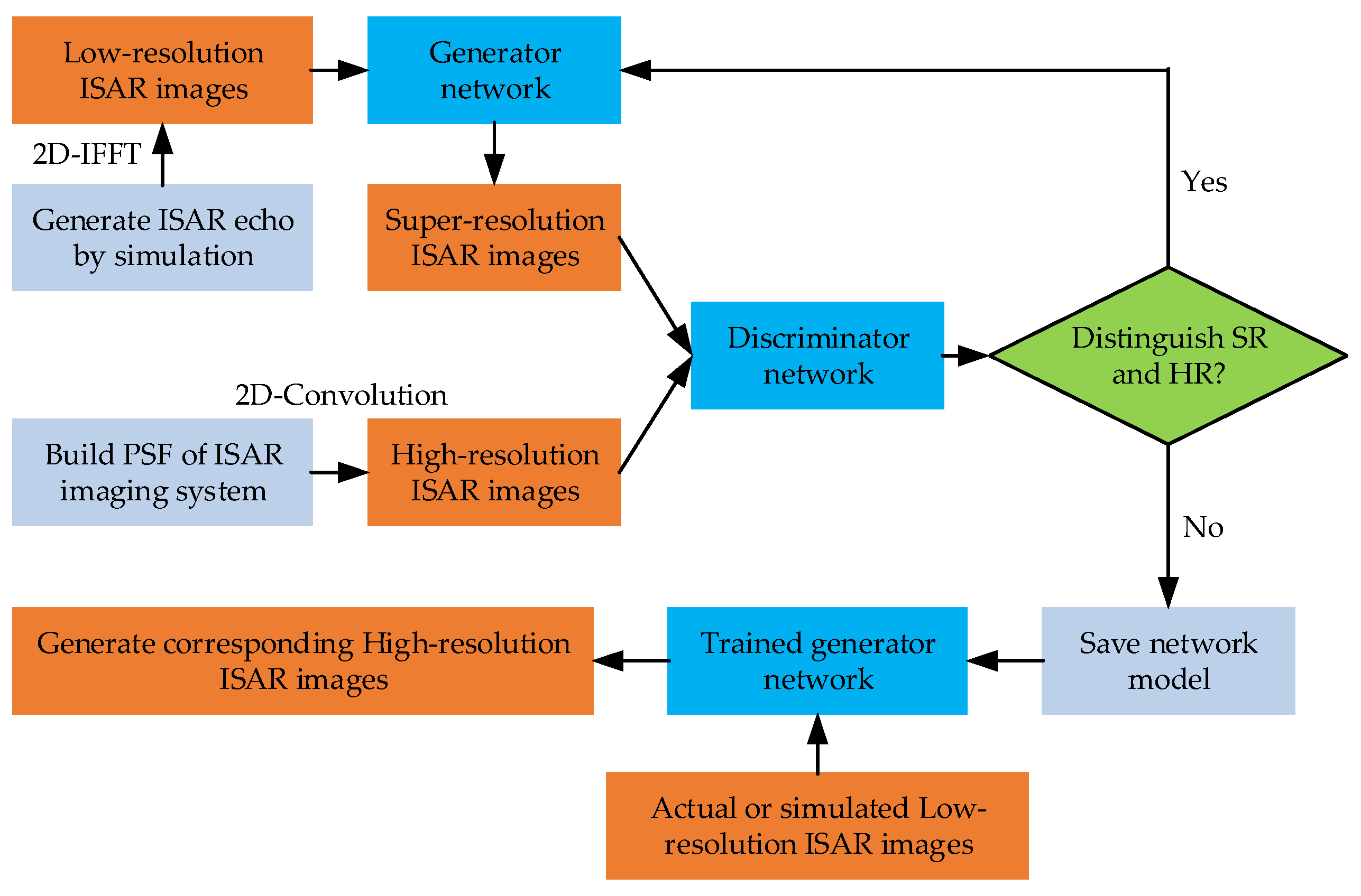
The GAN has a powerful processing capacity to improve the resolution of the ISAR images. The main mechanism lies in its strong end-to-end mapping learning ability, which reconstructs high-resolution (HR) images using low-resolution (LR) images by supervised learning. According to Equation (7), LR ISAR images can be obtained by taking the Inverse fast Fourier transform (IFFT) to the radar echo, while the HR ISAR images can be acquired by the convolution between target scattering function and PSF of HR ISAR system in Equation (8). The framework of the proposed GAN is shown in Figure 2.
The final purpose is to reconstruct the HR ISAR images based on LR ISAR images by the trained generator network. It can be transformed into an optimization problem shown in Equation (9):
where represents generator network, are LR ISAR images to input , are the outputs of , are real HR images corresponding to as labels, is the loss function of and stands for the network parameters set of . To achieve this goal, the training procedure continues until the generator network succeeds in fooling the discriminator network . In this situation, the resolution of will get improved and is the trained generator network that we will require.
To solve the optimization problem in (9), standard discriminator is adopted in [16], which is common for the GAN, shown in Equation (10):
where represents taking average value, is the distribution of HR ISAR images, and is the distribution of LR ISAR images. According to this criterion, adversarial loss is introduced into , which improves the ability to recover weak scatter points correctly for .
Different from literature [16], we replace the standard discriminator with the relativistic average discriminator (RaD) [22] to provide more target details, which can be represented by . In general, the standard discriminator describes whether the super-resolution (SR) ISAR image is real or fake, and the relativistic average discriminator estimates the probability that a HR ISAR image is more realistic than a SR ISAR image. Equations (11) and (12) show their definitions respectively:
where is the sigmoid function, is the output of non-transformed discriminator, and represents the operation of taking average value in mini batch. So, the discriminator loss can be expressed as:
Also, the adversarial loss for generator is:
3.2. Design of the Proposed GAN
For ISAR images, they do not have rich edges and color information like optical images. The most prominent feature of ISAR images is image contrast, which is displayed in the form of bright spots. Skip connections in the residual network (Res-Net) can preserve the image contrast [16], so we take Res-Net as the basic structure of . Inspired by [20], the architecture of is shown in Figure 3a. To improve the detailed expression ability of recovered ISAR images, the Residual-in-Residual Dense Block (RRDB) is adopted in the generator network. RRDB contains multi-level residual network and dense connections, which can describe the weak scatterers of ISAR images accurately and improve performance. Here, each RRDB contains three dense blocks and the number of RRDB is 11. A dense block is composed of four convolution layers and three leaky rectified linear unit (LeakyRelu) layers. The convolution layer consists of kernels and 64 feature maps with stride 1 [20], which can improve network performance. Also, batch normalization (BN) layers in dense blocks are removed [23]. Besides, is residual scaling to prevent instability and the value of is 0.2. Different from the image super-resolution task, our training data, namely HR images and LR images, have the same size. And LR images are not obtained by down sampling in the data generation stage. So, the up-sampling module is cancelled to fit our task. The final convolution layer contains three output channels.
The generator has a strong representation ability, the corresponding network structure of discriminator is shown in Figure 3b. First, and pass through a convolution layer (3 channels and 64 feature maps) with a kernel and stride 1. A leaky ReLU with a constant value of 0.2 is followed. Then consecutive convolution, BN, and leaky ReLU is used. Number of filters starts with 64 and consecutively increases by 128, 256, and 512. Next, two dense layers are used with output channel 1024 and 1. A leaky ReLU is also used between them. Finally, a sigmod activation function is selected to estimate whether is more realistic than .
3.3. Loss Function
The form of a loss function is vital for the generator to get the SR ISAR images. In various networks, different designs have improved the performance of the images, especially the Peak Signal-to-Noise Ratio (PSNR) value. These PSNR-oriented approaches often select the MSE as the loss function, which can be expressed as:
where and represent the height and width of HR/SR ISAR images, respectively. However, the results of MSE optimization problems are often over-smoothed, which will make some weak scatterers disappear and the overall performance of SR ISAR images get worse [20].
Instead of using MSE loss, we select the absolute loss to enhance the resolution of the SR ISAR images to get a better performance, which can be given as:
At the same time, we introduce the feature loss into to maintain the main characteristics of scattering points. Feature loss is based on the ReLU layers of the pre-trained VGG19 network. We use to represent the features obtained by the j-th convolution before the i-th maxpooling layer. In this article, we select to get the feature loss [20], which can be defined as:
In addition, the adversarial loss is also introduced into to recover the detailed features of weak scatter points shown in Equation (14). Therefore, the definition of is:
where and are the coefficients to balance and . In ISAR images, the amplitude of most areas is close to zero except for some strong scattering points. So, the values of and shuold be selected reasonably.
4. Processing Details
4.1. Data Acquisition
First, we randomly generate some scatterers in a specified area to obtain the radar echo. As mentioned before, LR ISAR images can be obtained by taking IFFT to the radar echo. The corresponding HR ISAR images can be acquired by convolving target scattering function with PSF. Here, the PSF is approximated by a 2-D Gaussian function instead of the Sinc function and its expression is shown in Equation (19):
where and control the azimuth and range resolution, respectively. Then under the condition of no noise and full aperture, the LR ISAR images and HR ISAR images are the inputs and annotations of the proposed GAN, respectively.
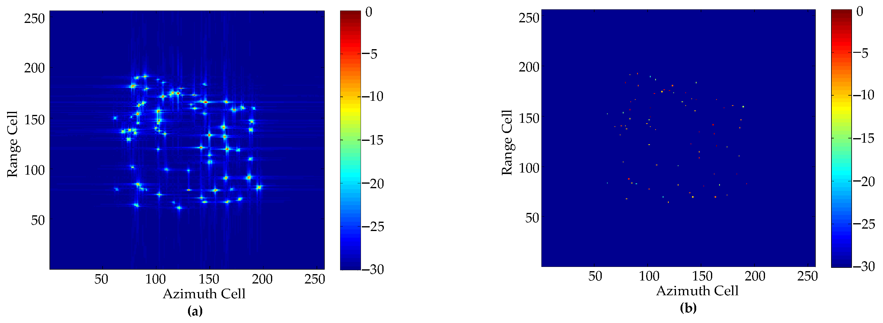
In the generation stage of training data, the related parameters are as follows: radar carrier frequency 10 GHz, bandwidth 400 MHz, pulse repetition frequency 400 Hz, pulse width μs, and pulse number 256. Each pulse contains 256 samples and 10–200 points are randomly generated in an area with a width of 50. The different scattering coefficients obey the standard complex Gaussian distribution. We obtain the LR/HR ISAR images by the MATLAB and the size of images is set to . The images are displayed in log magnitude with a dynamic range of 30 dB. The 10,000 LR/HR ISAR image pairs are used to train the proposed GAN. The randomly selected input and annotation image in training process are shown in Figure 4.
The training process can be divided into two steps. First, we only select the absolute loss in Equation (16) as the loss function for initialization, which can help the generator obtain the pleasing SR ISAR images. Then we use the in Equation (18) to optimize the network with and [20]. The training process is performed using an NVIDIA V100 GPU based on PyTorch. The Adam is adopted as our optimization algorithm with , [20]. The batch size is 4 and the learning rate is [20]. We alternately train the generator and discriminator network of the proposed GAN for 5 epochs, which costs 6.5 h.
4.2. Testing Strategy
In the test part, [16] has compared the performance of CV-CNN and Res-Net, so we only select three different GAN networks to compare with the method proposed in this paper, which can be simply defined as GAN1, GAN2, and GAN3. The network structure of GAN1 and GAN2 is the same as that in literature [16], but they adopt different loss functions. In GAN1, the loss function is [24], where is the adversarial loss adopting the standard discriminator . In GAN2, the loss function is , shown in Equation (18). As for GAN3, the network structure uses the structure proposed in this paper, but its loss function is , where .
To quantitatively evaluate the performance of different methods, we adopt three metrics, namely PSNR, structural similarity (SSIM), and image entropy (IE). Supposing that the annotation image is recorded as and the reconstructed image is recorded as , the definitions of these metrics are as follows [25]:
where is maximum pixel value of , and are the mean value of and , and are the variance of and , is the covariance of and , and . Among the above three metrics, we search to obtain a bigger PSNR, a bigger SSIM, and a smaller IE for the better reconstructed image.
5. Experiment Results and Analysis
In the experiment part, we select simulated data and measured data to verify the performance of different methods. In most articles, the number of scattering points for simulated aircraft is relatively small. While in our experiment, simulated aircraft data consists of 276 scattering points. The relevant parameters of simulated data are the same as those of the training network. Measured data contains the Yak42 aircraft data and F-16 airplane model data. The carrier frequency and bandwidth of the Yak42 aircraft data are 5.52 GHz and 400 MHz, respectively. The F-16 airplane model is measured in the microwave chamber. The frequency range is from 34.2857 to 37.9428 GHz.
Under the conditions of no noise and full aperture, we compare the performance of different methods. Then we consider the influence of random Gaussian noise on ISAR imaging performance for different methods. The random Gaussian noise is added to the radar echo for simulated data and measured data. The corresponding SNR is 2 and −4 dB. Next, the different methods are tested under the condition of sparse aperture. The echo data of LR ISAR images needs to be under-sampled. Here, we just consider that 224 pulses are recorded. In addition, zero padding is used to obtain test pictures. Finally, the universality and generalization of the proposed GAN are verified by the F-16 airplane model data.
For the complexity of different networks, the training process of the proposed GAN and GAN3 all cost 6.5 h, while GAN1 and GAN2 cost 3 h. Because of this, the proposed GAN adopts a more complex network structure. For the trained networks, the imaging time of the proposed GAN and GAN3 is 0.51 s, while the imaging time of GAN1 and GAN2 is 0.46 s.
5.1. Comparison of No Noise and Full Aperture
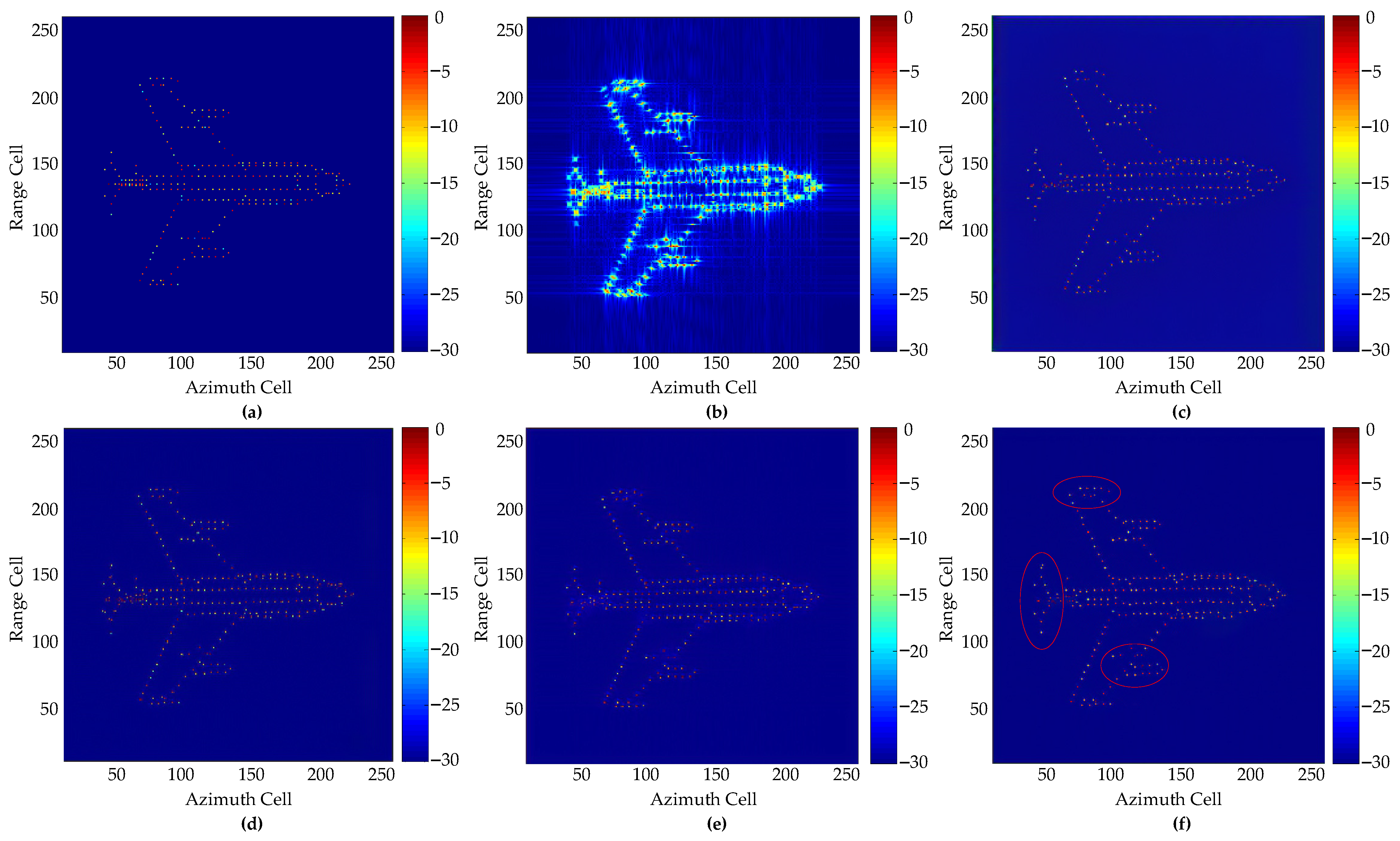
The imaging results of simulated aircraft by different methods are shown in Figure 5 under the condition of no noise and full aperture. The corresponding metrics are presented in Table 1. A LR ISAR image is shown in Figure 5b. We can see that its resolution is limited, and strong sidelobes submerge many weak scattering points. It is observed that four different methods all get better imaging performance than IFFT, which indicates the superiority of GAN. The proposed GAN has the smallest IE, and acceptable PSNR and SSIM. From Figure 5f, it is visually obvious that the proposed GAN has the best resolution performance and correctly reconstructs the most weak scattering points, compared with other methods. The proposed GAN describes the target details correctly, such as the tails of simulated aircraft. Compared with Figure 5d,f, we can see that the reconstructed result from GAN2 recovers some weak points incorrectly, which shows that the network structure proposed in this paper is better than that in [16]. Compared with Figure 5c,d, we can find that GAN2 achieves better performance than GAN1 precisely because the loss function proposed in this paper is adopted, which shows the effectiveness of the proposed loss function. In addition, the metrics of GAN3 are not bad, but Figure 5e has some unpleasant shadows around scattering points. Meanwhile, in Figure 5f the ISAR image has sharp edges. So, it is verified that loss has better performance than MSE loss in ISAR images.
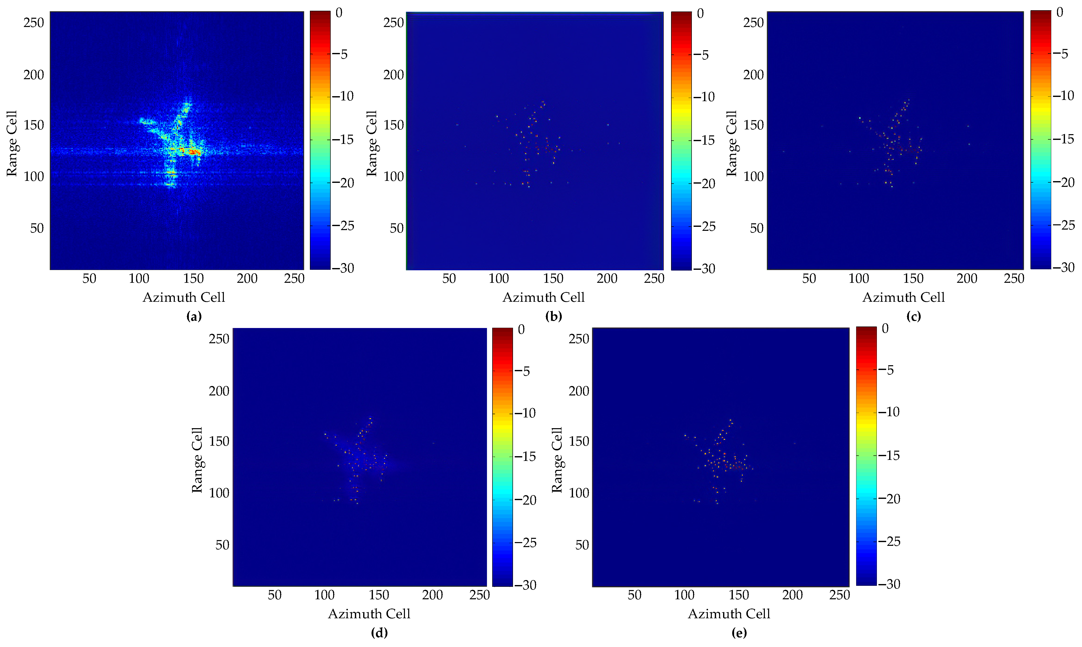
The imaging results of Yak42 by different methods are shown in Figure 6. The corresponding metrics are shown in Table 2. As can be seen from Figure 6a, the imaging result of the traditional method is not focused and has many strong sidelobes. Compared with other methods, the proposed GAN obtains the better-focused image and gets the smallest IE. At the same time, the proposed GAN does not produce many fake points, while the imaging results of GAN1 and GAN2 have some fake points in the background. Just like the simulated aircraft experiment, GAN2 has better imaging effect than GAN1, which further confirms the effectiveness of the proposed loss function. In addition, the imaging result of GAN3 is over-smoothed and has shadows in the background, which also confirms that the MSE loss is not good.
5.2. Comparison of Different SNRs
The imaging results of simulated aircraft under different SNRs are shown in Figure 7 and Figure 8. The corresponding metrics are shown in Table 3 and Table 4. The proposed GAN gets the smallest IE, the highest SSIM, and acceptable PSNR when SNR is 2 dB and −4 dB. As shown in Figure 8f, the ISAR image formed by the proposed GAN is focused with a clearer background even when SNR is −4 dB. The proposed GAN improves resolution significantly. At the same time, it can recover the target details as much as possible. Of course, it is inevitable to lose some scattering points information. While for other ISAR images, there are some fake points appearing in the background because of the strong noise. This can prove the superiority of the proposed method. Similarly, GAN2 has better performance than GAN1 because of the proposed loss function. GAN3 has shadows around the target because of the MSE loss.
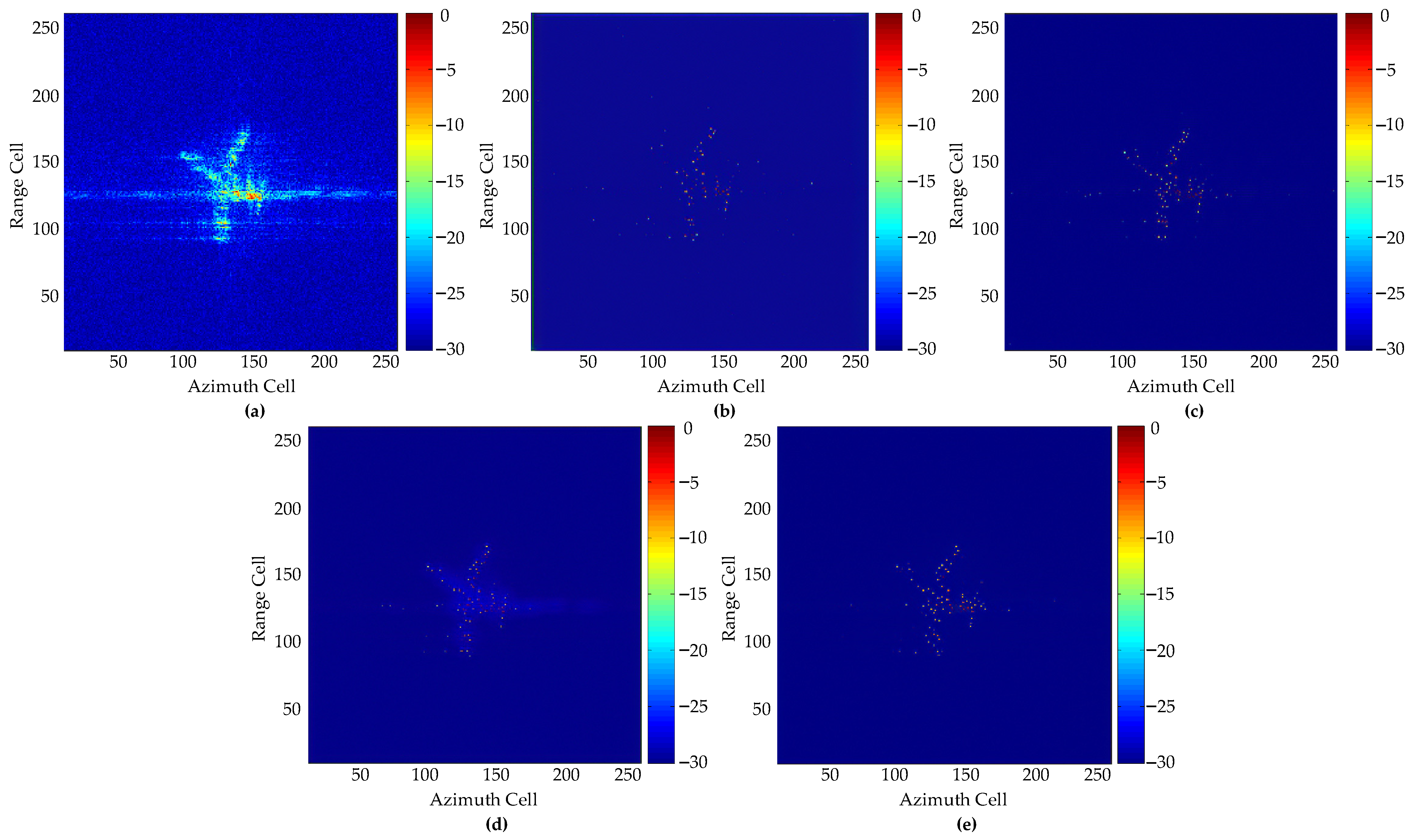
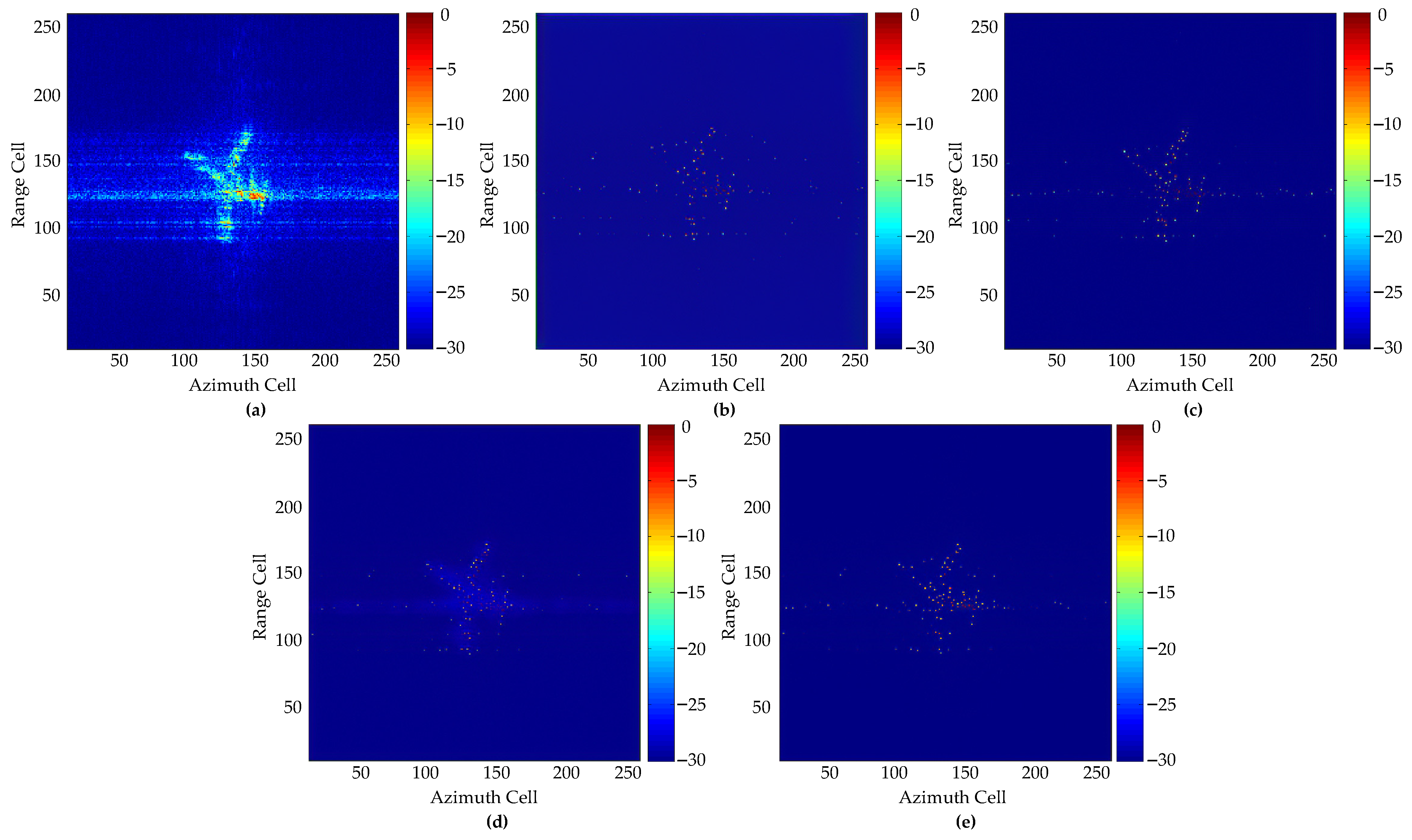
The imaging results of Yak42 under different SNRs are shown in Figure 9 and Figure 10. The corresponding metrics are shown in Table 5 and Table 6. The proposed GAN has the smallest IE. It can recover the target details correctly and improve the resolution of Yak42. The image quality does not degrade significantly with the decrease of SNR. The proposed GAN depicts the outline of Yak42 clearly, which is helpful for target recognition. In addition, it produces as few fake points as possible with a clear background, while for GAN1 and GAN2 some fake points still exist in the images. This phenomenon shows the effectiveness of the proposed method. In addition, the outline of Yak42 for GAN3 is blurred because of the MSE loss. The above analysis can show that the proposed GAN is not sensitive to low SNR.
5.3. Comparison of Sparse Aperture
The imaging results of simulated aircraft under SA are shown in Figure 11. The corresponding metrics are shown in Table 7. It can be seen from Figure 11b that the ISAR image of IFFT does not have good focusing performance. The scattering points are seriously defocused in azimuth direction. The proposed GAN gets the smallest IE, the highest SSIM and PSNR. The proposed GAN improves resolution significantly and describes more target details. Weak scattering points are recovered as much as possible by the proposed GAN. However, some weak scattering points inevitably vanish because of the existence of SA. Compare with other ISAR images, Figure 11f does not generate many fake points around the target. For other networks, there are many fake points in the background. So, the proposed GAN gets the better imaging performance.
The imaging results of Yak42 under SA are shown in Figure 12. The corresponding metrics are shown in Table 8. The proposed GAN has the smallest IE. It recovers more target details than other networks and improves resolution performance of Yak42. However, some fake points appear around the target, which shows the proposed GAN is sensitive to SA. Similarly, GAN2 has better imaging performance than GAN1 because of the proposed loss function. The ISAR image of GAN3 has a blurred outline of Yak42, which is the result of using MSE loss.
5.4. Universality and Generalization of the Proposed GAN
To validate the universality and generalization of the proposed GAN, an all-metal scaling model of an F-16 is measured in the microwave chamber, as shown in Figure 13a. From Figure 13b, we can see that the proposed GAN improves the resolution performance and has a clear outline of the F-16. However, it does not describe scattering characteristics of the F-16 perfectly. In fact, the carrier frequency of training data is different from Yak42 in previous experiments, which also proves the universality and generalization of the proposed GAN.
6. Conclusions
A resolution enhancement method for ISAR imaging based on GAN is proposed in this paper. We adopt a relativistic average discriminator (RaD) to improve the ability to describe target details. The Residual-in-Residual Dense Block (RRDB) is used in the generator network. The loss function consists of feature loss, adversarial loss, and absolute loss. Feature loss is used to maintain the main characteristics of ISAR images. Adversarial loss is introduced to recover the weak scattering points. Absolute loss can make ISAR images not over-smoothed. Compared with other networks, the simulation shows that the proposed GAN can improve resolution performance significantly and describes the target details well. At the same time, the proposed GAN produces as few fake points as possible. In addition, it can work well under the condition of different SNRs. The proposed GAN is sensitive to sparse aperture, which will be improved in the future work. Besides, the universality and generalization of the proposed GAN are also well verified.
Author Contributions
Conceptualization and methodology, H.W.; software, H.W.; resources, Q.Z. and Y.L.; writing—review and editing, H.W., K.L., X.L., Q.Z., Y.L. and L.K. All authors have read and agreed to the published version of the manuscript.
Funding
This research was funded by the National Nature Science Foundation of China under Grant 62131020 and the Natural Science Basic Research Program of Shaanxi under Grant 2020JQ-480.
Institutional Review Board Statement
Not applicable.
Informed Consent Statement
Not applicable.
Data Availability Statement
Not applicable.
Acknowledgments
The authors would like to thank all reviewers and editors for their comments on this paper.
Conflicts of Interest
The authors declare no conflict of interest.
References
- Kang, L.; Luo, Y.; Zhang, Q.; Liu, X.W.; Liang, B.S. 3-D Scattering Image Sparse Reconstruction via Radar Network. IEEE Trans. Geosci. Remote Sens. 2022, 60, 5100414. [Google Scholar] [CrossRef]
- Xue, R.H.; Bai, X.R.; Zhou, F. SAISAR-Net: A Robust Sequential Adjustment ISAR Image Classification Network. IEEE Trans. Geosci. Remote Sens. 2021, 60, 5214715. [Google Scholar] [CrossRef]
- Bai, X.R.; Zhang, Y.; Zhou, F. High-resolution radar imaging in complex environments based on Bayesian learning with mixture models. IEEE Trans. Geosci. Remote Sens. 2019, 57, 972–984. [Google Scholar] [CrossRef]
- Deng, L.K.; Zhang, S.H.; Zhang, C.; Liu, Y.X. A multiple-input multiple-output inverse synthetic aperture radar imaging method based on multidimensional alternating direction method of multipliers. J. Radars. 2021, 10, 416–431. [Google Scholar]
- Liu, X.W.; Dong, C.; Luo, Y.; Kang, L.; Liu, Y.; Zhang, Q. Sparse Reconstruction for Radar Imaging Based on Quantum Algorithms. IEEE Geosci. Remote Sens. Lett. 2022, 19, 3507905. [Google Scholar] [CrossRef]
- Cai, T.T.; Wang, L. Orthogonal Matching Pursuit for Sparse Signal Recovery with Noise. IEEE Trans. Inf. Theory 2011, 57, 4680–4688. [Google Scholar] [CrossRef]
- Mohimani, H.; Babaie-Zadeh, M.; Jutten, C. A Fast Approach for Overcomplete Sparse Decomposition Based on Smoothed Norm. IEEE Trans. Signal Process. 2009, 57, 289–301. [Google Scholar] [CrossRef] [Green Version]
- Li, S.; Amin, M.; Zhao, G.; Sun, H. Radar imaging by sparse optimization incorporating MRF clustering prior. IEEE Geosci. Remote Sens. Lett. 2020, 17, 1139–1143. [Google Scholar] [CrossRef] [Green Version]
- Zhang, S.H.; Liu, Y.X.; Li, X. Computationally Efficient Sparse Aperture ISAR Autofocusing and Imaging Based on Fast ADMM. IEEE Trans. Geosci. Remote Sens. 2020, 58, 8751–8765. [Google Scholar] [CrossRef]
- Gao, J.K.; Deng, B.; Qin, Y.L.; Wang, H.Q.; Li, X. Enhanced Radar Imaging Using a Complex-Valued Convolutional Neural Network. IEEE Geosci. Remote Sens. Lett. 2019, 16, 35–39. [Google Scholar] [CrossRef] [Green Version]
- Hu, C.Y.; Wang, L.; Li, Z.; Zhu, D.Y. Inverse Synthetic Aperture Radar Imaging Using a Fully Convolutional Neural Network. IEEE Geosci. Remote Sens. Lett. 2020, 17, 1203–1207. [Google Scholar] [CrossRef]
- Gao, X.Z.; Qin, D.; Gao, J.K. Resolution enhancement for inverse synthetic aperture radar images using a deep residual network. Microw. Opt. Technol. Lett. 2020, 62, 1588–1593. [Google Scholar] [CrossRef]
- Yang, T.; Shi, H.Y.; Lang, M.Y.; Guo, J.W. ISAR imaging enhancement: Exploiting deep convolutional neural network for signal reconstruction. Int. J. Remote Sens. 2020, 41, 9447–9468. [Google Scholar] [CrossRef]
- Qian, J.; Huang, S.Y.; Wang, L.; Bi, G.A.; Yang, X.B. Super-Resolution ISAR Imaging for Maneuvering Target Based on Deep-Learning-Assisted Time-Frequency Analysis. IEEE Trans. Geosci. Remote Sens. 2022, 60, 5201514. [Google Scholar] [CrossRef]
- Wei, X.; Yang, J.; Lv, M.J.; Chen, W.F.; Ma, X.Y.; Long, M.; Xia, S.Q. ISAR High-Resolution Imaging Method With Joint FISTA and VGGNet. IEEE Access. 2021, 9, 86685–86697. [Google Scholar] [CrossRef]
- Qin, D.; Gao, X.Z. Enhancing ISAR Resolution by a Generative Adversarial Network. IEEE Geosci. Remote Sens. Lett. 2021, 18, 127–131. [Google Scholar] [CrossRef]
- Li, R.Z.; Zhang, S.H.; Zhang, C.; Liu, Y.X.; Li, X. Deep Learning Approach for Sparse Aperture ISAR Imaging and Autofocusing Based on Complex-Valued ADMM-Net. IEEE Sens. J. 2021, 21, 3437–3451. [Google Scholar] [CrossRef]
- Wei, S.J.; Liang, J.D.; Wang, M.; Shi, J.; Zhang, X.L.; Ran, J.H. AF-AMPNet: A Deep Learning Approach for Sparse Aperture ISAR Imaging and Autofocusing. IEEE Trans. Geosci. Remote Sens. 2022, 60, 5206514. [Google Scholar] [CrossRef]
- Li, X.Y.; Bai, X.R.; Zhou, F. High-Resolution ISAR Imaging and Autofocusing via 2D-ADMM-Net. Remote Sens. 2021, 13, 2326. [Google Scholar] [CrossRef]
- Wang, X.T.; Yu, K.; Wu, S.X.; Gu, J.J.; Liu, Y.H.; Dong, C.; Qiao, Y.; Loy, C.C. ESRGAN: Enhanced Super-Resolution Generative Adversarial Networks. In Proceedings of the European Conference on Computer Vision Workshops, Munich, Germany, 8–14 September 2018. [Google Scholar]
- Özdemir, C. Inverse Synthetic Aperture Radar Imaging with Matlab Algorithms; Wiley: Hoboken, NJ, USA, 2012. [Google Scholar]
- Xing, X.R.; Zhang, D.W. Image-to-Image Translation using a Relativistic Generative Adversarial Network. In Proceedings of the 11th International Conference on Digital Image Processing, Guangzhou, China, 10–13 May 2019. [Google Scholar] [CrossRef]
- Lim, B.; Son, S.; Kim, H.; Nah, S.; Lee, K.M. Enhanced deep residual networks for single image super-resolution. In Proceedings of the 30th IEEE/CVF Conference on Computer Vision and Pattern Recognition Workshops, Honolulu, HI, USA, 21–26 July 2017; pp. 1132–1140. [Google Scholar] [CrossRef] [Green Version]
- Ledig, C.; Theis, L.; Huszar, F.; Caballero, J.; Cunningham, A.; Acosta, A.; Aitken, A.; Tejani, A.; Totz, J.; Wang, Z.H.; et al. Photo-Realistic Single Image Super-Resolution Using a Generative Adversarial Network. In Proceedings of the 30th IEEE/CVF Conference on Computer Vision and Pattern Recognition, Honolulu, HI, USA, 21–26 July 2017; pp. 105–114. [Google Scholar] [CrossRef] [Green Version]
- Zeng, C.Z.; Zhu, W.G.; Jia, X.; Yang, L. Sparse Aperture ISAR Imaging Method Based on Joint Constraints of Sparsity and Low Rank. IEEE Trans. Geosci. Remote Sens. 2021, 59, 168–181. [Google Scholar] [CrossRef]
Figure 1.
ISAR imaging model.

Figure 2.
Framework of the proposed GAN for ISAR resolution enhancement.

Figure 3.
The architecture of the proposed GAN for ISAR resolution enhancement: (a) the structure diagram of generator network; (b) the structure diagram of discriminator network.
Figure 3.
The architecture of the proposed GAN for ISAR resolution enhancement: (a) the structure diagram of generator network; (b) the structure diagram of discriminator network.


Figure 4.
An example of training data: (a) input image; (b) annotation image.

Figure 5.
Imaging results of simulated aircraft under the condition of no noise and full aperture: (a) Ground truth; (b) IFFT; (c) GAN1; (d) GAN2; (e) GAN3; (f) Proposed GAN.
Figure 5.
Imaging results of simulated aircraft under the condition of no noise and full aperture: (a) Ground truth; (b) IFFT; (c) GAN1; (d) GAN2; (e) GAN3; (f) Proposed GAN.

Figure 6.
Imaging results of Yak42 under the condition of no noise and full aperture: (a) IFFT; (b) GAN1; (c) GAN2; (d) GAN3; (e) Proposed GAN.
Figure 6.
Imaging results of Yak42 under the condition of no noise and full aperture: (a) IFFT; (b) GAN1; (c) GAN2; (d) GAN3; (e) Proposed GAN.

Figure 7.
Imaging results of simulated aircraft at SNR = 2 dB: (a) Ground truth; (b) IFFT; (c) GAN1; (d) GAN2; (e) GAN3; (f) Proposed GAN.
Figure 7.
Imaging results of simulated aircraft at SNR = 2 dB: (a) Ground truth; (b) IFFT; (c) GAN1; (d) GAN2; (e) GAN3; (f) Proposed GAN.

Figure 8.
Imaging results of simulated aircraft at SNR = −4 dB: (a) Ground truth; (b) IFFT; (c) GAN1; (d) GAN2; (e) GAN3; (f) Proposed GAN.
Figure 8.
Imaging results of simulated aircraft at SNR = −4 dB: (a) Ground truth; (b) IFFT; (c) GAN1; (d) GAN2; (e) GAN3; (f) Proposed GAN.

Figure 9.
Imaging results of Yak42 at SNR = 2 dB: (a) IFFT; (b) GAN1; (c) GAN2; (d) GAN3; (e) Proposed GAN.
Figure 9.
Imaging results of Yak42 at SNR = 2 dB: (a) IFFT; (b) GAN1; (c) GAN2; (d) GAN3; (e) Proposed GAN.

Figure 10.
Imaging results of Yak42 at SNR = −4 dB: (a) IFFT; (b) GAN1; (c) GAN2; (d) GAN3; (e) Proposed GAN.
Figure 10.
Imaging results of Yak42 at SNR = −4 dB: (a) IFFT; (b) GAN1; (c) GAN2; (d) GAN3; (e) Proposed GAN.

Figure 11.
Imaging results of simulated aircraft under sparse aperture: (a) Ground truth; (b) IFFT; (c) GAN1; (d) GAN2; (e) GAN3; (f) Proposed GAN.
Figure 11.
Imaging results of simulated aircraft under sparse aperture: (a) Ground truth; (b) IFFT; (c) GAN1; (d) GAN2; (e) GAN3; (f) Proposed GAN.

Figure 12.
Imaging results of Yak42 under sparse aperture: (a) IFFT; (b) GAN1; (c) GAN2; (d) GAN3; (e) Proposed GAN.
Figure 12.
Imaging results of Yak42 under sparse aperture: (a) IFFT; (b) GAN1; (c) GAN2; (d) GAN3; (e) Proposed GAN.

Figure 13.
Imaging results of F-16: (a) Original image in the microwave chamber; (b) Proposed GAN.


Table 1.
Numerical performance evaluation for simulated aircraft under ideal environment.
| Method | PSNR (dB) | SSIM | IE |
|---|---|---|---|
| IFFT | 15.9432 | 0.7001 | 4.3366 |
| GAN1 | 22.2503 | 0.7172 | 3.0268 |
| GAN2 | 26.7698 | 0.8458 | 2.0156 |
| GAN3 | 26.7794 | 0.8320 | 2.1744 |
| Proposed | 26.6372 | 0.8403 | 1.6376 |
Table 2.
Numerical performance evaluation for Yak42 under ideal environment.
| Method | IFFT | GAN1 | GAN2 | GAN3 | Proposed |
|---|---|---|---|---|---|
| IE | 3.8012 | 2.4514 | 1.5298 | 1.9007 | 1.3477 |
Table 3.
Numerical performance evaluation for simulated aircraft at SNR = 2 dB.
| Method | PSNR (dB) | SSIM | IE |
|---|---|---|---|
| IFFT | 16.8479 | 0.6560 | 4.4659 |
| GAN1 | 22.3841 | 0.7267 | 2.6676 |
| GAN2 | 26.1405 | 0.8434 | 1.9693 |
| GAN3 | 26.5236 | 0.8471 | 2.1149 |
| Proposed | 26.2321 | 0.8507 | 1.8374 |
Table 4.
Numerical performance evaluation for simulated aircraft at SNR = −4 dB.
| Method | PSNR (dB) | SSIM | IE |
|---|---|---|---|
| IFFT | 15.0749 | 0.1856 | 5.3295 |
| GAN1 | 22.9877 | 0.7218 | 2.7199 |
| GAN2 | 26.6015 | 0.8394 | 2.0603 |
| GAN3 | 26.8521 | 0.8432 | 2.1498 |
| Proposed | 26.6683 | 0.8511 | 1.6324 |
Table 5.
Numerical performance evaluation for Yak42 at SNR = 2 dB.
| Method | IFFT | GAN1 | GAN2 | GAN3 | Proposed |
|---|---|---|---|---|---|
| IE | 3.9670 | 2.3316 | 1.5434 | 1.8926 | 1.4509 |
Table 6.
Numerical performance evaluation for Yak42 at SNR = −4 dB.
| Method | IFFT | GAN1 | GAN2 | GAN3 | Proposed |
|---|---|---|---|---|---|
| IE | 4.7616 | 2.3161 | 1.5685 | 1.8593 | 1.5270 |
Table 7.
Numerical performance evaluation for simulated aircraft under sparse aperture.
| Method | PSNR (dB) | SSIM | IE |
|---|---|---|---|
| IFFT | 15.7553 | 0.5048 | 4.8516 |
| GAN1 | 22.1140 | 0.6706 | 3.1566 |
| GAN2 | 25.6569 | 0.7975 | 2.1496 |
| GAN3 | 26.1744 | 0.8258 | 2.4644 |
| Proposed | 25.7515 | 0.8261 | 2.0390 |
Table 8.
Numerical performance evaluation for Yak42 under sparse aperture.
| Method | IFFT | GAN1 | GAN2 | GAN3 | Proposed |
|---|---|---|---|---|---|
| IE | 4.1299 | 2.5353 | 1.6230 | 2.0888 | 1.5077 |
Publisher’s Note: MDPI stays neutral with regard to jurisdictional claims in published maps and institutional affiliations. |
© 2022 by the authors. Licensee MDPI, Basel, Switzerland. This article is an open access article distributed under the terms and conditions of the Creative Commons Attribution (CC BY) license (https://creativecommons.org/licenses/by/4.0/).
Share and Cite
MDPI and ACS Style
Wang, H.; Li, K.; Lu, X.; Zhang, Q.; Luo, Y.; Kang, L. ISAR Resolution Enhancement Method Exploiting Generative Adversarial Network. Remote Sens. 2022, 14, 1291. https://doi.org/10.3390/rs14051291
AMA Style
Wang H, Li K, Lu X, Zhang Q, Luo Y, Kang L. ISAR Resolution Enhancement Method Exploiting Generative Adversarial Network. Remote Sensing. 2022; 14(5):1291. https://doi.org/10.3390/rs14051291
Chicago/Turabian StyleWang, Haobo, Kaiming Li, Xiaofei Lu, Qun Zhang, Ying Luo, and Le Kang. 2022. "ISAR Resolution Enhancement Method Exploiting Generative Adversarial Network" Remote Sensing 14, no. 5: 1291. https://doi.org/10.3390/rs14051291
Note that from the first issue of 2016, this journal uses article numbers instead of page numbers. See further details here.