
Delineation of Geomorphological Woodland Key Habitats Using Airborne Laser Scanning


Faculty of Environmental Sciences and Natural Resource Management, Norwegian University of Life Sciences, P.O. Box 5003, NO-1432 Ås, Norway
*
Author to whom correspondence should be addressed.
Remote Sens. 2022, 14(5), 1184; https://doi.org/10.3390/rs14051184
Submission received: 1 February 2022
/
Revised: 22 February 2022
/
Accepted: 25 February 2022
/
Published: 27 February 2022
(This article belongs to the Special Issue Feature Paper Special Issue on Ecological Remote Sensing)
Abstract
:Forest ecosystems provide a range of services and function as habitats for many species. The concept of woodland key habitats (WKH) is important for biodiversity management in forest planning standards and certification schemes. The main idea of the WKH is to preserve biodiversity hotspots in the forest landscape. Current methods used in delineating WKH rely on costly field inventories. Furthermore, it is well known that the surveyor introduces an error because of the subjective assessment. Remote sensing may reduce this error in a cost-efficient way. The current study develops automated methods using airborne laser scanning (ALS) data to delineate geomorphological WKH, i.e., rock walls and stream gorges. The methods were evaluated based on a complete field inventory of WKH in a 1600 ha area in south-eastern Norway. The delineated WKH showed high detection rates, minor omission errors, but high commissions errors. Combining the delineation into a map of potential WKH suitable to guide field surveyors resulted in detecting all field reference WKH, i.e., a detection rate of 100% and a commission error of 25%. It is concluded that a higher degree of automatization might be possible to improve results and increase the efficiency of WKH inventories.
1. Introduction
Forest ecosystems provide a range of services and are habitats for many species [1]. Forest management and activities influence the amount and quality of available habitats. In Europe, clear-felling is the primary driver of changes in forest ecosystems [2]. At the end of the last century, the impacts of forest management on biodiversity were recognized as an important issue. As a result, biodiversity management in forestry received increased attention [3], and the concept of woodland key habitats (WKH) was introduced as an addition to traditional forest protection in many countries, especially in the Nordic and Baltic countries [3,4,5].
The main idea of the WKH is to preserve small important biodiversity hotspots in the forest landscape [3]. The basic idea of the concept is that red-list species occur in clusters and are not randomly distributed in the forest landscape [6]. Thus, identifying the specific habitats where red-listed species are clustered provided an efficient and practical approach. The idea of delineating specific habitats was further incorporated into forest planning standards and certification schemes, such as Programme for the Endorsement of Forest Certification schemes (PEFC) and Forest Stewardship Council (FSC). Thus, routines and procedures for inventories of WKH were established [3,6]. These procedures are based on a field inventory and prior knowledge of the forest and consists of delineating pre-described habitats according to specified rules. The type and number of WKH vary substantially between countries, but some common groups of habitats exist. Timonen et al. [3] suggested that WKH in the Nordic and Baltic countries could be divided into seven main groups: (1) edaphic sites, (2) geomorphological sites, (3) hydrological sites, (4) sites based on dominating tree species and successional stage (mainly old stands with long continuity), (5) burned and other young successional stands developing after recent natural disturbances, (6) cultural biotopes, and (7) individual important trees. The methods used in delineating such WKH have experienced very little change during the last two decades and are still based on field inventories as a primary approach.
Contrary to the field-based methods applied for WKH inventories, forest-management inventories have changed drastically during the last two decades. Two decades ago, such inventories were based on intensive manual photointerpretation and field inventories. Nowadays, forest-management planning is mainly based on the combination of airborne laser scanning (ALS) and digital aerial imagery in many countries [7,8]. Combined with sample plots, important forest attributes such as timber volume, height, and basal area, are cost-effectively mapped over vast regions [9]. However, operationally delineating WKH is still based on extensive field inventories and benefits from remote sensing sources only to a limited degree, mainly from orthophotos. The subjectivity and, thus, differences between surveyors in assessing habitats is also a known problem that should be minimized [10,11]. Since remotely sensed data are already available for the forest management inventory, they are also available for WKH inventory; thus, the cost of incorporating these data into inventory protocols is minimal.
Remotely sensed data could be used in several ways to improve WKH inventories, for example, by performing a direct classification. In the remote sensing literature, there are documented methods for WKH related to deadwood [12,13,14], successional stages [15], special or old trees [16,17], areas with high herbaceous plant diversity [18,19] or hydrological features [20,21,22,23]. However, there are issues with the obtained accuracy, as some WKH can be modeled with small commission and omission errors, but other WKH types have significant errors of commission and omission, and thus remote sensing is less applicable. Nevertheless, using remote sensing to provide maps of potential WKH, preferably with small omission rates, that can be used as pre-information for field inventories is an appealing idea. The pre-information maps can guide the field crew to important locations, and the extent and attributes could be controlled. Such a use of remotely sensed data would provide a practical approach to overcome the issues related to the accuracy of remote-sensing products, while reducing the time and cost directed towards field inventories. In addition, the use of remote sensing may also provide more transparent, objective and predictable methods for WKH delineation. Hence, maps with potential WKH may also reduce the surveyor error inherent in the field inventories and provide a more objective and equal delineation between surveyors.
One of the seven main WKH groups is connected to geomorphological or topographical conditions. The WKH in the geomorphological group are rock walls, rock shelves, boulders, clay ravines, and stream gorges [3,6]. The humidity in these areas is essential for many species, and such spots act as habitats for many bryophytes and lichens [6]. The ALS technology used for the forest-management inventories was initially developed for terrain mapping, and there is extensive literature regarding the identification of landforms using such terrain data [20,21,24]. However, according to our knowledge, little has been done to identify biodiversity hotspots, such as WKH.
Remote sensing may also provide the attributes of delineated WKH either directly or by modeling. An essential criterion for valuing rock walls as a habitat for rare species is the aspect, which serves as a proxy for moisture. North or east-facing rock walls are often moister under Nordic conditions and typically have higher biodiversity, especially of red-listed bryophytes and lichens [25]. For stream gorges, the moistest areas are located in east or west-oriented habitats where sun radiation seldom reaches the gorge’s bottom.
The main objective of the current study was to develop methods using remotely sensed data to provide pre-information about the location and attributes of WKH. Specifically, we identified WKH connected to geomorphological conditions important for biodiversity in Norway using ALS. The two specific key habitats were rock walls and stream gorges. The identified areas were evaluated against reference data gathered manually in the field.
2. Materials and Methods
2.1. Study Area
The 1600 ha study area is located in the municipality of Gjøvik (60°55′ N, 10°34′ E, 300–600 m a.s.l.), Innlandet County, approximately 100 km north of Oslo, Norway (Figure 1). The area is actively managed and dominated by Norway spruce (Picea abies (L.) Karst.). Scots Pine (Pinus sylvestris L.) is found on dry ridges and mires, while deciduous species, mainly birch (Betula spp.), are scattered in the landscape.
2.2. Field Inventory
A traditional WKH field inventory was conducted in the study area during 2017 according to the updated field protocol for the Norwegian WKH inventories [26], which follows the EcoSyst framework [27]. Two different companies were involved in the inventory. Company A carried out the primary survey in subareas I and III (Figure 1). Furthermore, company B surveyed subarea I, using the same protocol. From the WKH, we used rock walls and stream gorges (Figure 1 and Figure 2). The field crew used a tablet with a simple global navigation satellite systems GNSS receiver in the WKH inventory. Thus, expected accuracy would be equal to what could be expected from mobile phones, likely around 5–13 m under optimal conditions [28] and larger errors are expected under closed forest canopies [29,30].
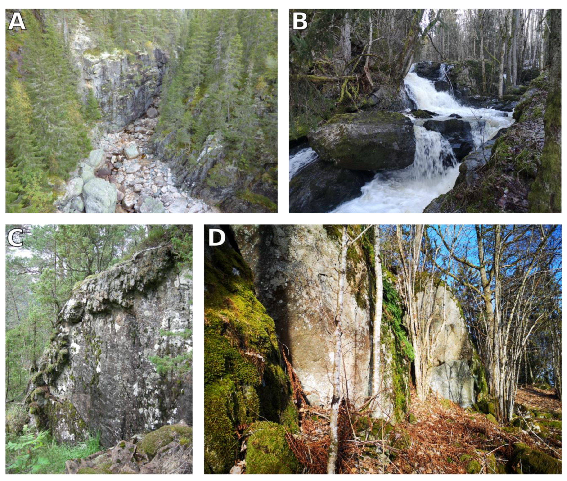
The majority of red-list species connected to rock walls require moist habitat. According to the WKH inventory protocol, a rock wall (Figure 2C,D) is defined as at least 3 m tall and with a slope of more than 80 degrees [26]. To be delineated, WKH usually have to reach a minimum size. However, there is no size requirement for rock walls stated in the protocol. The minimum area size for other WKH in Norway varies from 0.05 to 0.5 ha depending on the key habitat type [26]. Rock walls are often found in conjunction with stream gorges. Stream gorges are clear topographic landforms for which the stream provides moisture and humidity to the surrounding forest (Figure 2A,B). In addition, the stream carries nutrients, and thus richer vegetation types occur. According to the field protocol, stream gorges should be more than 25 m long, and the height from the bottom of the gorge to the top should be more than 5 m [26].
In total, 15 WKH were recorded by the two companies covering 21.51 ha (Table 1). The two companies identified nine rock walls covering 3.57 ha and six stream gorges covering 16.55 ha. Companies A and B recorded six and three rock walls in subarea I, respectively (Figure 1). None of the recorded rock-wall habitats overlapped. Company A recorded five stream gorges in both areas, while company B delineated one stream gorge. This stream gorge was also identified by company A in subarea I.
2.3. Remotely Sensed Data
ALS data were acquired on the 5th and the 15th of July 2018. The sensor was mounted on a fixed-wing aircraft flying at a maximum speed of 130 knots and approximately 900 m above ground level. The sensor used was the Leica ALS70-HP equipped with multiple pulses in air technology (MPiA) and operated at a wavelength of 1064 nm, with a pulse rate of two times 218.6 kHz and a scan angle of ±20°. It was flown with a side overlap of 44% and up to four returns per pulse were recorded, resulting in an average point density of 7.1 points m−2. The ground echoes were automatically classified using the progressive triangular irregular network-densification algorithm [31,32], implemented in the TerraScan software (Terrasolid Ltd., Helsinki, Finland).
2.4. Rock Wall Detection
First, a digital elevation model (DTM) was derived from triangulation irregular networks (TINs) from the ALS echoes classified as originating from the ground. Second, we computed the height difference within a three-by-three neighborhood window, i.e., maximum height minus minimum height. Raster cells with a height difference of more than 3 m were used to identify potential rock walls. We used three different resolutions of the DTM to detect possible rock walls. The resolutions were 0.27 m, 0.50 m, and 1 m, representing a slope in the three-by-three neighborhood of 79.8°, 71.6°, and 56.3°, respectively. Thus, by specifying the resolution and height difference we were able to account for both the slope and height threshold simultaneously as opposed to if we first had computed slope in an ordinary way [33] and then applied the height threshold. Third, for each DTM resolution, the potential rock wall pixels were identified and converted into polygons. A closing operation was performed on the polygons, i.e., a buffer of √2 m was applied to each of them, followed by a negative buffer of the same distance. Lastly, polygons smaller or equal to 250 m2 were removed from the potential rock walls. Furthermore, the potential rock walls derived from the different DTM resolutions were combined. The areas identified were given a score value representing an increased chance of correct identification. Initially, all areas identified with the 1 m resolution were given a score value of 3. Areas overlapping the delineation from a higher DTM resolution were updated, and scores of 2 (0.50 m) and 1 (0.27 m) were assigned. The length of the potential rock wall was derived from their minimum oriented bounding boxes [34].
2.5. Stream Gorges Detection
Stream gorges are a typical landform often visible in terrain models. To identify potential landforms that could be stream gorges, we used an ALS-derived DTM with a spatial resolution of 5 m to classify the area into different landforms. Using the methodology presented by Weiss (2001), we classified nine different landforms based on Topographic Position Index (TPI). The TPI compares the elevation in a raster cell to the mean elevation in a specified neighborhood. Thus, positive TPI values represent areas higher than their neighborhood, and negative TPI values represent areas that are comparatively lower. The TPI value and ecological interpretation vary according to the extent of the neighborhood used (Guisan et al., 1999). The combination of a small-scale and a large-scale TPI can be used to classify different landforms (Weiss 2001). A neighborhood of 50 m and 1000 m was used in this study based on preliminary trials and was assigned a score value of 1. Results of neighborhood combinations of 100 m and 1000 m and 300 m and 2000 m are also presented for comparison, with assigned score values of 2 and 3, respectively. Since elevation tends to have a spatial correlation, the range of TPI values increases with scale. Thus, we centered and standardized the TPI values. This allowed the use of the equations formulated by Weiss et al. [35] to classify the combinations of TPI grids. We used the canyons or deeply incised streams as the potential stream gorges areas from the landform classification.
Stream gorges were defined as at least 5 m deep and longer than 25 m. Thus, we used a stream network to evaluate the depth and length of the potential stream gorges. In the current study, we used the official river network of Norway from the Norwegian Water Resources and Energy Directorate. The stream height was derived from each raster cell of the 1 m DTM intersecting the stream. Similarly, the height of the border of the potential stream gorges was found. Then, each point at the stream was assigned the value of the spatially nearest height of the potential stream gorge border points. The difference between the stream height and the nearest stream gorge border height at 1 m resolution was computed. All points with a difference greater than 5 m and separated with less than 20 m were converted to individual line segments. The segments longer than 25 m (length criteria) were buffered using a 75 m buffer with a flat end, i.e., representing the maximum width of the stream gorge. The potential stream gorges intersecting with the buffer were maintained. Thus, areas that did not fulfill the depth criteria were removed.
2.6. Woodland Key Habitat Aspect
The aspect was computed within the field-recorded WKH. The computed aspect values were compared to the field-assessed value of the aspect. Since the ALS point cloud was readily available, we utilized it to compute the aspect instead of relying on raster-based methods. Raster-based methods introduce issues regarding decisions for parameters such as raster cell size, window size to compute aspect and how to aggregate individual cells for a delineated unit. Thus, we fitted the following linear model to the ground ALS echoes within each delineated unit:
where Z is the height of the ALS echo, X and Y are the east and north coordinates, , and are parameters to be estimated, is the model error. Thus, the changes in Z based on X and Y are modeled and used to compute the aspect:
where and . The value is converted to the compass direction in the interval 0–360°, according to the following rule:
- if aspect < 0
- WKHaspect = 90 − aspect
- else if aspect > 90
- WKHaspect = 360 − aspect + 90
- else
- WKHaspect = 90 − aspect
Furthermore, the WKHaspect was converted to the four aspect classes recorded in the Norwegian WKH inventory: North (WKHaspect ≥ 315 & <45), East (WKHaspect ≥ 45 & <135), South (WKHaspect ≥ 135 & <225) and West (WKHaspect ≥ 225 & <315).
2.7. Accuracy Assessment
The results were evaluated based on the detection rate (both delineated in the field and computed from ALS data), omission error (field delineated WKH, but not found using the ALS data) and commission error (WKH identified using ALS data, but not identified in the field) [36]. A WKH was considered to have been detected using ALS data if the identified area intersected with the ground reference WHK map. The aspect was evaluated by comparing the ALS-derived and field recorded values. The agreement of aspect values was summarized with error matrices.
3. Results
3.1. Woodland Key Habitat Detection
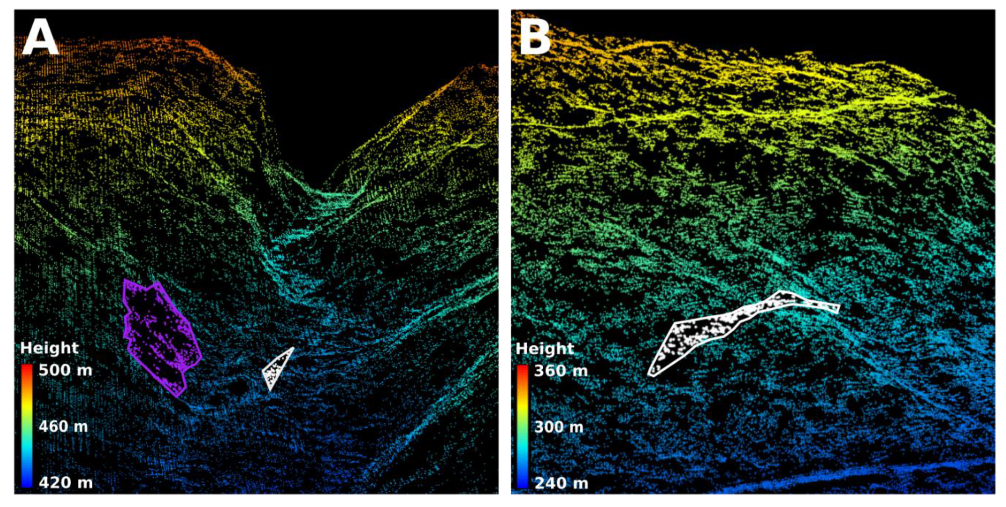
During rock-wall detection, 492 areas were identified. Thus, commission errors were found to be large when using the initial detection. However, removing areas smaller than 250 m2 reduced the number of identified areas to 39 without influencing the detection rate and omission errors (Table 2). The field reference data were based on manual delineation and are not error-free. Using the ALS-derived DTM, we found that two reference polygons were prone to errors. First, one of the polygons seemed inaccurately positioned in field. This represents correct detection in the field, but with a location error of approximately 15–20 m (Figure 3A). The rock wall is situated in a gorge where GNSS signals might be poor because of high canopy cover [29,30] and terrain forms preventing GNSS signals reaching the receiver. Second, a polygon is erroneously delineated on a flat area and thus cannot be a rock wall (Figure 3B). By correcting field data for these two polygons and recalculating the detection rate and errors of omission and commission, all rock walls were detected with a score value of 2. However, the number of commissions is approximately four times larger than the number of detected rock walls. Hence, the commission errors are larger than desired. Many of these identified rock walls were associated with stream gorges. Stream gorges can be narrow, and rock walls naturally appear on the sides of the stream gorge. Thus, computing the errors based on both types of WKH reduced commission errors significantly (Table 3), thereby decreasing the erroneously automatically identified areas to less than 10.
The applied method provided a large detection rate for stream gorges (Table 4). Five out of six field-recorded stream gorges were identified. The omitted stream gorge had two sections deeper than 5 m of the ground reference gorge boundary. These sections were 21.2 m and 31.4 m long, respectively. Consequently, the depth and length criteria were fulfilled. This stream gorge was missed because it was classified as midslope drainage or shallow valley in the landform classification. However, one area was identified inside the omitted stream gorge using the procedure to detect rock walls. Thus, by combining the identified stream gorges and rock walls, the field crew would have visited all the ground reference stream gorges. The number of commission errors was six. Of these, three were located in areas with few or no trees. Thus, we could use a normalized digital surface model, or a canopy cover proxy derived from the ALS data to remove these. One of the commission errors delineated seems relevant as a stream-gorges habitat.
3.2. Woodland Key Habitat Aspect
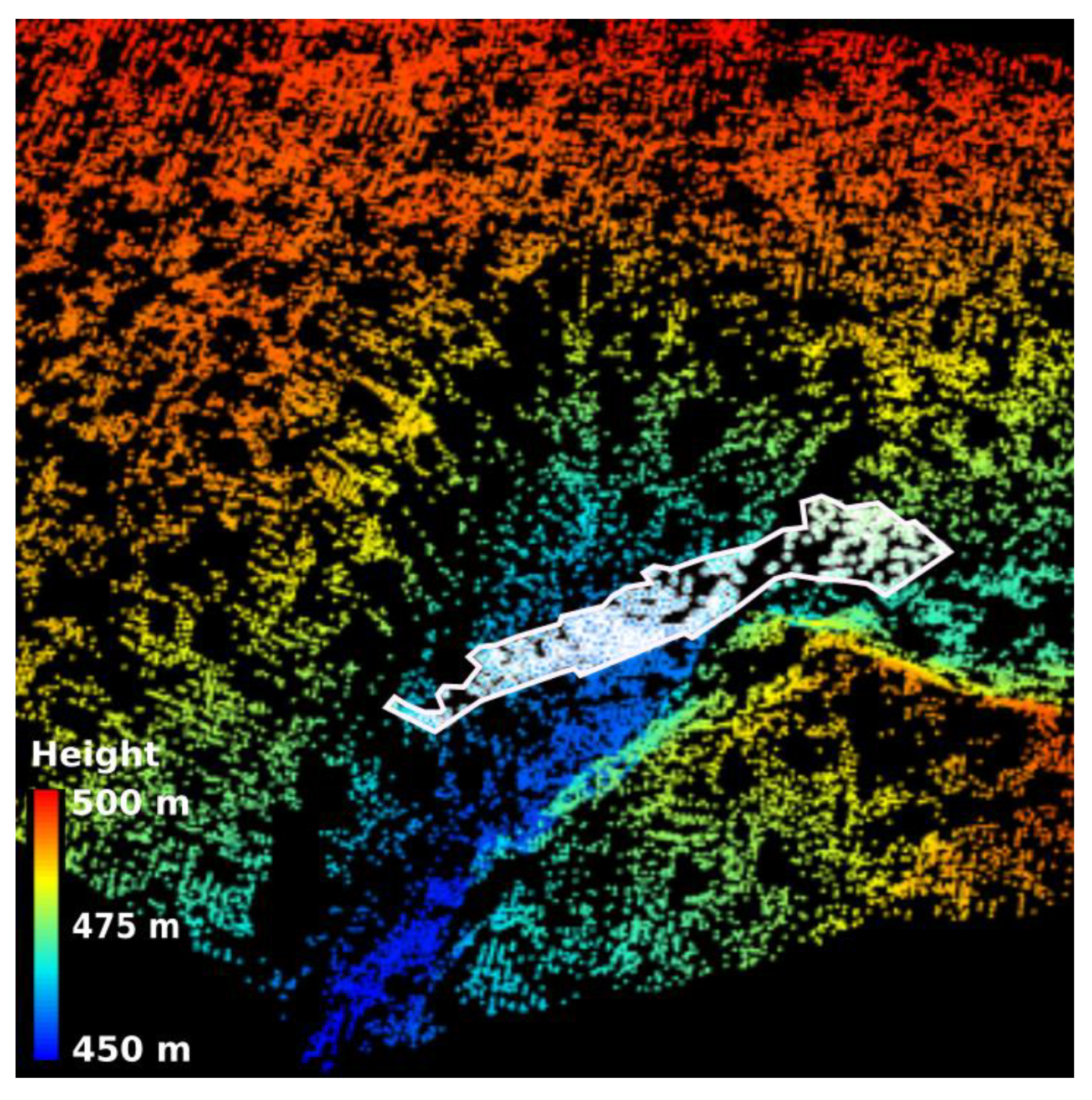
The ALS computed aspect values calculated for the ground referenc rock walls revealed that four of the rock walls assessed as north-facing were east-facing when aspects were computed from ALS data (Table 5). There was an agreement in both field and ALS-derived aspect for one south-facing rock wall. Furthermore, one of the west-facing rock walls was calculated to be east-facing. However, the inspection of the ALS points used to calculate the aspect revealed that this error was caused by a mislocation of the ground reference data (Figure 4). The rock wall is situated in a stream gorge and includes a higher area towards the west. Thus, the computed values would be east-facing, correct for parts of the rock wall. The calculated aspect for stream gorge habitat was in agreement with the field assessment in all classes, of which three were north-facing, and three were east-facing (Table 5).
4. Discussion
The current study produced a map with pre-information about the location, extent and attributes of WKH (Figure 5). The agreement with the ground reference data was good in terms of detection rate, and omission errors were limited. The WKH in the geomorphological group are among the easiest to delineate using ALS data. Furthermore, ALS is commonly used in forest inventories and thus is readily available over vast areas. The difference between observers in vegetation and habitat mapping is a known problem [10,11]. Thus, the pre-information maps seem to be a promising tool to improve delineation and minimize differences between observers.
However, the current study presents some limitations, caused, among other things, by the limited number of field WKH. Nevertheless, the dataset is unique as a complete WKH map covering the entire area is seldom available. The quality of the field reference could also be questioned as some of the commission errors seem reasonable, but of course, other features such as forest structure, e.g., thinnings, may have led to the sites not being mapped in the field. Additionally, it is clear from the ALS data (Figure 3 and Figure 4) that geolocation issues in the digitization of WKH during the field inventory, including erroneous delineations, might be present.
We used an existing stream network that is not necessarily available in all areas or countries. Using this network instead of a DTM-derived stream network has benefits as it is part of an official map layer and thus is quality controlled. Nevertheless, a DTM-derived stream network could provide an option if an official network is absent. However, careful editing of the point clouds close to barriers such as bridges and culverts is necessary to avoid incorrect stream identification.
The idea that the ALS-based pre-information represents a correct observation if it intersects with a WKH from the field inventory might be ambitious. However, it is reasonable to assume that guiding the field crew to a potential location would result in a correct delineation. Thus, we believe that a map of pre-information would reduce the time consumption for field work. However, if the editing work on the preliminary boundary is extensive, this might not be the case. However, combining the ALS delineation of rock walls and stream gorges into one map leads to detecting all ground reference WKH, i.e., a detection rate of 100%. In addition, the resulting commission errors were reduced to five additional areas to be visited during the field inventory for a commission rate of approximately 25%. Thus, the number of sites to visit in the field (i.e., area to check) to delineate the WKH becomes considerably reduced.
The high commission errors represent a potential problem, but there are reasonable explanations for such mistakes, as mentioned above. First, the commission errors might have occurred in areas with forest cover or forest structure unsuitable for WKH delineation, e.g., clear-cut or young forests. Thus, other environmental qualities of the site are evaluated subjectively in the field and were found not to support a WKH. Using the vegetation returns from the ALS to compute crown coverage or the successional stage could potentially reduce some of these errors [15,37]. Second, they could represent correct delineation and omission using the field inventory since field inventory for the entire area can be difficult. Furthermore, rock walls represent smaller geomorphological features that the field crew could easily oversee in dense forests. However, the main idea in the current study is that these ALS-based delineations guide the field crew to potential sites before being accepted as a WKH, thus, making the high commission errors reasonable.
The current study concerned two WKH, namely, rock walls and stream gorges. In Norway, clay ravines are also a defined type of WKH, and in Scandinavian and Baltic countries, rock shelves, boulders, steep bluffs, etc., are found in the geomorphological group of WKH. The methods presented in this study can be modified to fit specific WKH definitions for a range of related habitats such as clay ravines and other landforms connected to the terrain slope. However, the accuracy needs to be evaluated for the specific WKH.
Aspect classes were derived for all field recorded habitats, and agreement was evaluated. The aspect class was also computed and added to the pre-information WKH map (Figure 5). The point-based method applied to the ALS ground point cloud ensures that the computed aspect represents the entire WKH. The overall result seems to be that the field crew indicated a north-facing aspect while the ALS-based aspect was computed to be east-facing. A reasonable explanation could be that the field crew had issues determining the correct aspect direction either through subjective decisions or experienced problems with the compass in field. Another reason is that the field crew could integrate a more general assessment of the aspect direction by evaluating surrounding areas or placing more weight on some parts of the WKH. Thus, field crews could better assess the scale to which aspect should be derived. Providing the aspect on the pre-information map would support such assessments.
The current study showed that directly translating a field inventory protocol might be challenging when developing a remote sensing product such as this. In the present study, the definitions regarding size or length of a rock wall were found to be missing. Furthermore, a stream gorge or a rock wall that has been harvested and is now clear-cut will dry out, and thus it would be less moist and less valuable as a habitat. There are requirements regarding suitable forest cover and structure, but the field manual does not explicitly state this. In the field, the surveyor should assess the requirements subjectively. An objective description of such requirements would benefit further automatization through remote sensing.
We believe that a considerable amount of time could be saved during field inventories if the field crew has access to such pre-information maps on tablets (Figure 5). The maps will guide the field crew to important areas without necessarily influencing detection accuracy. Furthermore, an expected result is improved geolocation and a better agreement between different field crews. Pre-delineated WKH borders can be accepted in the field; thus, errors caused by hand drawing on tablets, positional errors, and subjectivity are minimized.
5. Conclusions
The current study developed ALS data methods to identify geomorphological WKH, i.e., rock walls and stream gorges. A map of potential WKH that can be used as pre-information in the field inventory was developed. The delineation showed high detection rates, low omission errors, and a high number of commissions. The field inventory of WKH used in the current study presented some potential issues with the delineation. It underlined the need for more objective tools, as developed in this study, to support field inventories. Furthermore, a method to compute aspect, a critical WKH attribute, provided good results. Overall, the methods and evaluations presented indicate that a higher degree of automatization is possible to improve outcomes and increase the efficiency of WKH inventories.
Author Contributions
Conceptualization, H.O.Ø.; methodology, H.O.Ø. and J.C.-B.; formal analysis, H.O.Ø.; investigation, H.O.Ø. and J.C.-B.; data curation, M.-C.J.-P., J.C.-B. and H.O.Ø.; writing—original draft preparation, H.O.Ø.; writing—review and editing, M.-C.J.-P., J.C.-B. and T.G.; visualization, H.O.Ø.; supervision, H.O.Ø.; project administration, H.O.Ø.; funding acquisition, H.O.Ø. and T.G. All authors have read and agreed to the published version of the manuscript.
Funding
This research was funded by the project PreMiNa, “Evaluation of remotely sensed data as pre-information for woodland key habitat inventories according to the EcoSyst framework”, and the project NOBEL, “Novel business models and mechanisms for the sustainable supply of and payment for forest ecosystem services”. The PreMiNa project is funded by the private research fund Skogtiltaksfondet, the forest trust fund (Utviklingsfondet for skogbruket), and private forest associations in Norway. The project NOBEL is supported under the umbrella of ERA-NET Cofund ForestValue. ForestValue has received funding from the European Union’s Horizon 2020 research and innovation program under grant agreement N° 773324. Furthermore, the NOBEL project was supported by the Norwegian Research Council (project number 297883).
Institutional Review Board Statement
Not applicable.
Informed Consent Statement
Not applicable.
Data Availability Statement
Restrictions apply to the availability of these data. Data were obtained from the Norwegian Agricultural Agency and are available from the authors with the permission of the Norwegian Agricultural Agency.
Acknowledgments
The authors would like to thank Terratec AS Norway for collecting and processing the ALS data. We also like to thank the Norwegian Agriculture Agency for organizing and sharing the ground reference data. Furthermore, we are grateful for the constructive and valuable comments from three anonymous reviewers and the academic editor on a previous version of the manuscript.
Conflicts of Interest
The authors declare no conflict of interest. The funders had no role in the design of the study; in the collection, analyses, or interpretation of data; in the writing of the manuscript, or in the decision to publish the results.
References
- Brockerhoff, E.G.; Barbaro, L.; Castagneyrol, B.; Forrester, D.I.; Gardiner, B.; González-Olabarria, J.R.; Lyver, P.O.; Meurisse, N.; Oxbrough, A.; Taki, H.; et al. Forest Biodiversity, Ecosystem Functioning and the Provision of Ecosystem Services. Biodivers. Conserv. 2017, 26, 3005–3035. [Google Scholar] [CrossRef] [Green Version]
- Curtis, P.G.; Slay, C.M.; Harris, N.L.; Tyukavina, A.; Hansen, M.C. Classifying Drivers of Global Forest Loss. Science 2018, 361, 1108–1111. [Google Scholar] [CrossRef] [PubMed]
- Timonen, J.; Siitonen, J.; Gustafsson, L.; Kotiaho, J.S.; Stokland, J.N.; Sverdrup-Thygeson, A.; Mönkkönen, M. Woodland Key Habitats in Northern Europe: Concepts, Inventory and Protection. Scand. J. For. Res. 2010, 25, 309–324. [Google Scholar] [CrossRef] [Green Version]
- Nitare, J.; Norén, M. Nyckelbiotoper Kartläggs i Nytt Projekt Vid Skogsstyrelsen [Woodland Key-Habitats of Rare and Endangered Species Will Be Mapped in a New Project of the Swedish National Board of Forestry]. Sven. Bot. Tidskr. 1992, 86, 219–226. [Google Scholar]
- Baumann, C.; Gjerde, I.; Blom, H.H.; Sætersdal, M.; Nilsen, J.-E.; Løken, B.; Ekanger, I. Environmental Inventories in Forests—Biodiversity. A Manual for Conducting Inventories of Forest Habitats. Part 1: Background and Principles; Skogforsk: Uppsala, Sweden, 2002; ISBN 9788280830050. [Google Scholar]
- Gjerde, I.; Sætersdal, M.; Blom, H.H. Complementary Hotspot Inventory—A Method for Identification of Important Areas for Biodiversity at the Forest Stand Level. Biol. Conserv. 2007, 137, 549–557. [Google Scholar] [CrossRef]
- Næsset, E. Area-Based Inventory in Norway—From Innovation to an Operational Reality. In Forestry Applications of Airborne Laser Scanning; Maltamo, M., Næsset, E., Vauhkonen, J., Eds.; Springer: Dordrecht, The Netherlands, 2014; pp. 215–240. [Google Scholar]
- Maltamo, M.; Packalen, P. Species-Specific Management Inventory in Finland. In Forestry Applications of Airborne Laser Scanning; Maltamao, M., Næsset, E., Vauhkonen, J., Eds.; Managing Forest Ecosystems; Springer: Dordrecht, The Netherlands, 2014; pp. 241–252. ISBN 9789401786621. [Google Scholar]
- Eid, T.; Gobakken, T.; Næsset, E. Comparing Stand Inventories for Large Areas Based on Photo-Interpretation and Laser Scanning by Means of Cost-plus-Loss Analyses. Scand. J. For. Res. 2004, 19, 512–523. [Google Scholar] [CrossRef]
- Haga, H.E.E.S.; Nilsen, A.B.; Ullerud, H.A.; Bryn, A. Quantification of Accuracy in Field-based Land Cover Maps: A New Method to Separate Different Components. Appl. Veg. Sci. 2021, 24, e12578. [Google Scholar] [CrossRef]
- Eriksen, E.L.; Ullerud, H.A.; Halvorsen, R.; Aune, S.; Bratli, H.; Horvath, P.; Volden, I.K.; Wollan, A.K.; Bryn, A. Point of View: Error Estimation in Field Assignment of Land-Cover Types. Phytocoenologia 2018, 49, 135–148. [Google Scholar] [CrossRef] [Green Version]
- Zielewska-Büttner, K.; Adler, P.; Kolbe, S.; Beck, R.; Ganter, L.M.; Koch, B.; Braunisch, V. Detection of Standing Deadwood from Aerial Imagery Products: Two Methods for Addressing the Bare Ground Misclassification Issue. For. Trees Livelihoods 2020, 11, 801. [Google Scholar] [CrossRef]
- Pesonen, A.; Maltamo, M.; Eerikäinen, K.; Packalèn, P. Airborne Laser Scanning-Based Prediction of Coarse Woody Debris Volumes in a Conservation Area. For. Ecol. Manag. 2008, 255, 3288–3296. [Google Scholar] [CrossRef]
- Martinuzzi, S.; Vierling, L.A.; Gould, W.A.; Falkowski, M.J.; Evans, J.S.; Hudak, A.T.; Vierling, K.T. Mapping Snags and Understory Shrubs for a LiDAR-Based Assessment of Wildlife Habitat Suitability. Remote Sens. Environ. 2009, 113, 2533–2546. [Google Scholar] [CrossRef] [Green Version]
- Falkowski, M.J.; Evans, J.S.; Martinuzzi, S.; Gessler, P.E.; Hudak, A.T. Characterizing Forest Succession with Lidar Data: An Evaluation for the Inland Northwest, USA. Remote Sens. Environ. 2009, 113, 946–956. [Google Scholar] [CrossRef] [Green Version]
- Korhonen, L.; Salas, C.; Østgård, T.; Lien, V.; Gobakken, T.; Næsset, E. Predicting the Occurrence of Large-Diameter Trees Using Airborne Laser Scanning. Can. J. For. Res. 2016, 46, 461–469. [Google Scholar] [CrossRef] [Green Version]
- Saynajoki, R.; Packalén, P.; Maltamo, M.; Vehmas, M.; Eerikainen, K. Detection of Aspens Using High Resolution Aerial Laser Scanning Data and Digital Aerial Images. Sensors 2008, 8, 5037–5054. [Google Scholar] [CrossRef] [PubMed] [Green Version]
- Vehmas, M.; Eerikäinen, K.; Peuhkurinen, J.; Packalén, P.; Maltamo, M. Identification of Boreal Forest Stands with High Herbaceous Plant Diversity Using Airborne Laser Scanning. For. Ecol. Manag. 2009, 257, 46–53. [Google Scholar] [CrossRef]
- Hakkenberg, C.R.; Zhu, K.; Peet, R.K.; Song, C. Mapping Multi-Scale Vascular Plant Richness in a Forest Landscape with Integrated LiDAR and Hyperspectral Remote-Sensing. Ecology 2018, 99, 474–487. [Google Scholar] [CrossRef]
- White, B.; Ogilvie, J.; Campbell, D.M.H.; Hiltz, D.; Gauthier, B.; Chisholm, H.K.H.; Wen, H.K.; Murphy, P.N.C.; Arp, P.A. Using the Cartographic Depth-to-Water Index to Locate Small Streams and Associated Wet Areas across Landscapes. Can. Water Resour. J. 2012, 37, 333–347. [Google Scholar] [CrossRef]
- Pirotti, F.; Tarolli, P. Suitability of LiDAR Point Density and Derived Landform Curvature Maps for Channel Network Extraction. Hydrol. Process. 2010, 24, 1187–1197. [Google Scholar] [CrossRef]
- Smeeckaert, J.; Mallet, C.; David, N.; Chehata, N.; Ferraz, A. Large-Scale Classification of Water Areas Using Airborne Topographic Lidar Data. Remote Sens. Environ. 2013, 138, 134–148. [Google Scholar] [CrossRef]
- Höfle, B.; Vetter, M.; Pfeifer, N.; Mandlburger, G.; Stötter, J. Water Surface Mapping from Airborne Laser Scanning Using Signal Intensity and Elevation Data. Earth Surf. Processes Landf. 2009, 34, 1635–1649. [Google Scholar] [CrossRef]
- Janowski, L.; Tylmann, K.; Trzcinska, K.; Rudowski, S.; Tegowski, J. Exploration of Glacial Landforms by Object-Based Image Analysis and Spectral Parameters of Digital Elevation Model. IEEE Trans. Geosci. Remote Sens. 2021, 60, 4502817. [Google Scholar] [CrossRef]
- Baumann, C.; Gjerde, I.; Blom, H.H.; Sætersdal, M.; Nilsen, J.-E.; Løken, B.; Ekanger, I. Environmental Inventories in Forests—Biodiversity. A Manual for Conducting Inventories of Forest Habitats Part 4: Guidelines for Ranking and Selection; Skogforsk and the Norwegian Ministry of Agriculture: Ås, Norway, 2002. [Google Scholar]
- Landbruksdirektoratet. Veileder for Kartlegging Av MiS-Livsmiljøer Etter NiN; VEILEDER VERSJON 1.0, JUNI 2017; Landbruksdirektoratet: Oslo, Norway, 2017; p. 26. [Google Scholar]
- Halvorsen, R.; Skarpaas, O.; Bryn, A.; Bratli, H.; Erikstad, L.; Simensen, T.; Lieungh, E. Towards a Systematics of Ecodiversity: The EcoSyst Framework. Glob. Ecol. Biogeogr. 2020, 29, 1887–1906. [Google Scholar] [CrossRef]
- Zandbergen, P.A. Accuracy of IPhone Locations: A Comparison of Assisted GPS, WiFi and Cellular Positioning. Trans. GIS 2009, 13, 5–25. [Google Scholar] [CrossRef]
- Tomaštík, J.; Varga, M. Practical Applicability of Processing Static, Short-Observation-Time Raw GNSS Measurements Provided by a Smartphone under Tree Vegetation. Measurement 2021, 178, 109397. [Google Scholar] [CrossRef]
- Reutebuch, S.E.; McGaughey, R.J.; Andersen, H.E.; Carson, W.W. Accuracy of a High-Resolution LIDAR Terrain Model under a Conifer Forest Canopy. Can. J. Remote Sens. 2003, 29, 527–535. [Google Scholar] [CrossRef]
- Axelsson, P. DEM Generation from Laser Scanner Data Using Adaptive TIN Models. Int. Arch. Photogramm. Remote Sens. 2000, 33, 111–118. [Google Scholar]
- Axelsson, P. Processing of Laser Scanner Data—Algorithms and Applications. ISPRS J. Photogramm. Remote Sens. 1999, 54, 138–147. [Google Scholar] [CrossRef]
- Burrough, P.A.; McDonell, R.A. Principles of Geographical Information Systems; Oxford University Press: New York, NY, USA, 1998; p. 190. [Google Scholar]
- Toussaint, G.T. Solving Geometric Problems with the Rotating Calipers. In Proceedings of the IEEE MELECON’83, Athens, Greece, 24–26 May 1983; Volume 83, p. A10. Available online: cs.swarthmore.edu (accessed on 1 February 2022).
- Weiss, A.D. Topographic Position and Landforms Analysis. In Proceedings of the Poster Presentation, ESRI User Conference, San Diego, CA, USA, 9–13 July 2001; Volume 200. Available online: jennessent.com (accessed on 1 February 2022).
- Foody, G.M. Status of Land Cover Classification Accuracy Assessment. Remote Sens. Environ. 2002, 80, 185–201. [Google Scholar] [CrossRef]
- Korhonen, L.; Korpela, I.; Heiskanen, J.; Maltamo, M. Airborne Discrete-Return LIDAR Data in the Estimation of Vertical Canopy Cover, Angular Canopy Closure and Leaf Area Index. Remote Sens. Environ. 2011, 115, 1065–1080. [Google Scholar] [CrossRef]
Figure 1.
Study area and location of field delineated rock walls and stream gorges.

Figure 2.
Examples of stream gorges (A,B) and rock walls (C,D). Pictures not from the study area. Photos by Rune Halvorsen licensed CC-BY-4.0 (A,C) and Hans Ole Ørka (B,D).
Figure 2.
Examples of stream gorges (A,B) and rock walls (C,D). Pictures not from the study area. Photos by Rune Halvorsen licensed CC-BY-4.0 (A,C) and Hans Ole Ørka (B,D).

Figure 3.
Errors in ground reference data. (A) The field observed rock wall assumed to be mislocated and (B) the field observed rock wall assumed to be wrong. ALS ground points are colored using height. Identified rock walls are colored white if recorded in the field and purple if identified automatically.

Figure 4.
Locations of points used to calculate aspect for one west-facing rock wall where ALS ground points are colored using height and identified rock wall is colored white when matching ground reference data.
Figure 4.
Locations of points used to calculate aspect for one west-facing rock wall where ALS ground points are colored using height and identified rock wall is colored white when matching ground reference data.

Figure 5.
Pre-information map of potential rock walls and stream gorges in the extended study area. Letters refer to aspect; N = north, E = east, S = south, and W = west.
Figure 5.
Pre-information map of potential rock walls and stream gorges in the extended study area. Letters refer to aspect; N = north, E = east, S = south, and W = west.


Table 1.
Summary of field delineated rock walls and stream gorges by the two companies.
| WKH | Company | n | Total Area (ha) | Mean Area (ha) | Area Range (ha) |
|---|---|---|---|---|---|
| A | 6 | 3.54 | 0.59 | 0.02–2.65 | |
| Rock walls | B | 3 | 0.03 | 0.02 | 0.00–0.02 |
| Total | 9 | 3.57 | 0.40 | 0.00–2.65 | |
| A | 5 | 15.93 | 3.19 | 0.40–6.84 | |
| Stream gorges | B | 1 | 2.01 | 2.01 | - |
| Total | 6 | 17.94 | 2.99 | 0.40–6.84 |
Table 2.
Detection rate, errors of omission and commission errors for rock walls (>250 m2) with different score values compared to ground reference data (rock walls). The numbers in the parenthesis are presented with the corrected field reference data.
Table 2.
Detection rate, errors of omission and commission errors for rock walls (>250 m2) with different score values compared to ground reference data (rock walls). The numbers in the parenthesis are presented with the corrected field reference data.
| Score | Detection Rate | Omission Errors | Commission Errors |
|---|---|---|---|
| 1 | 5 (6) | 4 (2) | 17 |
| 2 | 7 (8) | 2 (0) | 9 |
| 3 | 7 (8) | 2 (0) | 1 |
Table 3.
Detection rate, errors of omission and commission errors for rock walls (>250 m2) with different score values compared to ground reference data (rock walls and stream gorges). The numbers in the parenthesis are presented with corrected field reference data.
Table 3.
Detection rate, errors of omission and commission errors for rock walls (>250 m2) with different score values compared to ground reference data (rock walls and stream gorges). The numbers in the parenthesis are presented with corrected field reference data.
| Score | Detection Rate | Omission Errors | Commission Errors |
|---|---|---|---|
| 1 | 10 (11) | 5 (3) | 6 |
| 2 | 12 (13) | 3 (1) | 2 |
| 3 | 12 (13) | 3 (1) | 1 |
Table 4.
Detection rate, errors of omission and commission errors for stream gorges with different score values compared to ground reference stream gorge data.
Table 4.
Detection rate, errors of omission and commission errors for stream gorges with different score values compared to ground reference stream gorge data.
| Score | Detection Rate | Omission Errors | Commission Errors |
|---|---|---|---|
| 1 | 5 | 1 | 5 |
| 2 | 5 | 1 | 9 |
| 3 | 4 | 2 | 13 |
Table 5.
Comparison of ALS-derived and ground reference aspect for rock walls and stream gorges.
| ALS Aspect | Ground Reference Aspect | |||
|---|---|---|---|---|
| North | East | South | West | |
| North | 3 | |||
| East | 4 | 3 | 1 1 | |
| South | 1 | |||
| West | 1 | |||
1 The observation represents error based on geolocation in Figure 4.
Publisher’s Note: MDPI stays neutral with regard to jurisdictional claims in published maps and institutional affiliations. |
© 2022 by the authors. Licensee MDPI, Basel, Switzerland. This article is an open access article distributed under the terms and conditions of the Creative Commons Attribution (CC BY) license (https://creativecommons.org/licenses/by/4.0/).
Share and Cite
MDPI and ACS Style
Ørka, H.O.; Jutras-Perreault, M.-C.; Candelas-Bielza, J.; Gobakken, T. Delineation of Geomorphological Woodland Key Habitats Using Airborne Laser Scanning. Remote Sens. 2022, 14, 1184. https://doi.org/10.3390/rs14051184
AMA Style
Ørka HO, Jutras-Perreault M-C, Candelas-Bielza J, Gobakken T. Delineation of Geomorphological Woodland Key Habitats Using Airborne Laser Scanning. Remote Sensing. 2022; 14(5):1184. https://doi.org/10.3390/rs14051184
Chicago/Turabian StyleØrka, Hans Ole, Marie-Claude Jutras-Perreault, Jaime Candelas-Bielza, and Terje Gobakken. 2022. "Delineation of Geomorphological Woodland Key Habitats Using Airborne Laser Scanning" Remote Sensing 14, no. 5: 1184. https://doi.org/10.3390/rs14051184
Note that from the first issue of 2016, this journal uses article numbers instead of page numbers. See further details here.