Polarization Estimation with a Single Vector Sensor for Radar Detection

Abstract

Target detection using radar has important applications in military and civilian fields. Aimed at targets containing interference, radar polarimetry can facilitate discrimination between the target and interference. Since existing methods require the utilization of interference signals without targets in advance, they have a poor effect on interference with variable polarization. To solve this problem, this paper proposes a novel synchronous method to estimate the parameters of interference. First, we introduce a definition of the pulse compression signal-to-noise ratio, and prove that it is the polarization invariant in the virtual polarization adaptation. Then, for signals containing a target, interference, and noise, we propose a novel synchronous estimation method. Subsequently, we propose the two-dimensional golden selected method to further optimize the method with minimum calculation, and prove that the method presented in this paper is convergent and globally optimal. Finally, we analyze the presented method from three aspects: robustness, complexity, and applicability; the results of which demonstrate the efficacy of the method presented in this paper.

1. Introduction

Radar can obtain a target’s distance, speed, azimuth, and other information by transmitting electromagnetic waves and receiving echoes. In a complex environment, factors such as clutter, overlapping spectrum, and man-made interference can seriously affect the performance of radar. Among them, jamming interference is a very common and efficient method. For discrimination of target and interference, scholars have performed significant research and achieved good results in the time domain, spatial domain, and frequency domain [1,2,3,4]. However, some interfering devices (i.e., eigital radio frequency memory), can quickly identify radar signals and transmit interference with similar spectrums in the main lobe.This leads to poor results with existing methods in the time domain, spatial domain, and frequency domain. Polarization reflects the vector characteristics of an electromagnetic wave. Thanks to the outstanding contributions of Sinclair, Kennaugh, Huynen, and others [5,6,7], the research on electromagnetic waves has been extended from the time-domain, spatial-domain, and frequency-domain to the polarization-domain.

1.1. Summary of Relevant Literature

Radar anti-interference methods based on polarization originated in the 1970s, with the adaptive polarization canceler and multi-notch logic multiplication activation filter. Subsequently, in order to improve detection performance, the optimization problem was studied based on the signal interference-to-noise ratio and the power difference of signal and interference criteria, comprehensively considering the signal and interference power. For multiple-input multiple-output radar, References [8,9,10] utilized its waveform diversity and distributed antennas to achieve spatial diversity, so as to obtain a target’s angle and polarization information. However, these methods assume that the target and the interference are not in same range cell. For high-frequency surface wave radar, Mao [11] proposed a null phase-shift polarization filter that can not only suppress interference, but can also avoid the loss of target information. Subsequently, References [12,13,14,15] presented significant work on the oblique projection polarization filter. For monopulse radar, Wang et al. [16,17,18,19,20,21,22] estimated the parameters of signals containing only interference, and then performed polarization filtering on the signals containing the target and interference by weight coefficients. For warning radar, References [23,24,25] used multiple pulse signals with different azimuths to establish observation equations, and then estimated the target parameters based on the least squares. For interference suppression in the main lobe, the above-mentioned references make certain assumptions, which are as follows.

• References [11,12,13,14,15] required a prior knowledge of information on the target or the interference, i.e., a polarization and covariance matrix.
• References [8,9,16,17,18,19,20,21,23,24,25] assumed that the target and the interference were not at same range cell; i.e., these methods needed secondary data.

In general, the aforementioned methods, i.e., [8,9,16,17,18,19,20,21,23,24,25], all utilize the interference suppression method under asynchronization (to simplify the representation, hereinafter it is denoted as ISMA) and have some shortcomings. For example, when the interference is variable polarization, ISMA cannot achieve better suppression performance on the current interference, since it needs to estimate the polarization parameters of the previous interference. Therefore, the main goal of this paper is to suppress jamming interference under synchronization, which belongs to the interference suppression method under synchronization (to simplify the representation, hereinafter it is denoted as ISMS). In order to suppress jamming interference based on polarization, it is necessary to obtain the parameters of polarization. Therefore, this paper aims at the estimation of the polarization parameters, which are significant for suppressing interference. As for the estimation of the polarization parameters, Reference [26] proposed a method for estimating five-dimensional polarization-space-time channel parameters, which was applied for the public network. As for radar detection, Reference [27] analyzed regularized covariance estimation in compound Gaussian Sea clutter, which was based on synthetic aperture radar. For the one-dimensional signal of radar, it is well-known that parameter estimation methods based on eigenvalue decomposition, i.e., the estimation of signal parameters via rotational invariance techniques (ESPRIT) and multiple signal classification (MUSIC), all belong to ISMS. Many references have performed meaningful research on parameter estimation using ISMS.

1.

Nehorai and Paldi [28,29] first introduced a six-dimensional vector sensor and proposed a direction estimation method based on the vector cross-product, and then deduced mean-square angular error and covariance of vector angular error as performance measures. Subsequently, Reference [30] analyzed parameter estimation of a single incident wave in active/passive mode, and then characterized the best possible accuracy of unbiased estimators using the Cramér–Rao bound. References [31,32,33] analyzed the identifiability, uniqueness, and beamformer in vector sensors, respectively. References [34,35] focused on parameter estimation of partially polarized incident waves, which does not require a priori information about the array system such as sensor positions. References [36,37] estimated the parameters for signals of completely polarized waves and incompletely polarized waves. Reference [38] identified and tracked multiple wideband signals based on Reference [39].

2.

Li and Compton [40] first applied the ESPRIT-based method to a six-dimensional vector sensor, which could achieve angle and polarization parameter estimation. Reference [41] proposed ESPRIT-based method for angle and polarization parameters using crossed dipoles. Based on Reference [41], References [42,43,44] improved the ESPRIT-based method for different situations. Reference [42] proposed an angle-only ESPRIT-based method to simplify computations; Reference [43] changed a uniform linear array to a square array, which can extend the angle estimation to two dimensions; and Reference [44] focused on the coherent signal and combined the ESPRIT algorithm with spatial smoothing techniques using a uniform linear array. Reference [45] proposed a maximum likelihood method for joint DOA and polarization estimation based on manifold separation, and Reference [46] also used maximum likelihood estimation to obtain the angle and polarization parameters of partially polarized waves. Reference [47] compared three estimation methods for polarization parameters with a prior knowledge of direction. Reference [48] proposed an asymptotically statistically efficient method of direction estimation for coherent signals.

3.

Zoltowski and Wong [37] first used the vector cross-product DOA estimator in the ESPRIT-based direction-finding scheme involving multiple vector sensors. References [37,49,50] all analyzed the sparse array to solve the problem of direction ambiguity in parameter estimation. Reference [51] extracted five invariants from the Poynting vector on the basis of Reference [40], thereby simplifying the computation of parameter estimation. Reference [39] decoupled the angle and polarization parameters using a vector sensor in order to reduce the four-dimension spectral search of MUSIC to two dimensions. References [52,53] all used dislocation arrays (i.e., the three dipoles and the three loops were located separately, instead of being collocated in a point-like geometry) to solve the coupling problem of electric field sensors and magnetic field sensors. Reference [54] proposed an optimized root-MUSIC method, which softens the conditions of the previous antenna-array; that is, the number, orientation, or types of antennas could vary from array grid point to array grid point.

1.2. Innovative Points of This Paper

In this paper, we propose a novel synchronous method to estimate the parameters of interference with variable polarization using a single vector sensor. The main innovations of this paper are as follows.

• Compared with References [8,9,11,12,13,14,15,16,17,18,19,20,21,23,24,25], the presented method in this paper only needs the data collected from the range cell under test, and does not resort to secondary data or prior knowledge of the target and interference. Therefore, the presented method can estimate the parameters of interference with variable polarization.
• As for a single vector using a crossed dipole, the received signals contain three signals: jamming interference, target echo, and noise. Due to this, the number of signals is greater than that of the receiving antennas, meaning that the polarization parameters cannot be estimated directly by the ESPRIT-based method [41,42,43,44]. Moreover, References [28,29,30,31,32,33,37,40,41,42,43,49,50,51,52,53,54] all assumed that incoming signals were uncorrelated, and their performance degraded rapidly as the incident signals became highly correlated. However, the presented method can combine the polarization invariant and waveform information to solve the above problem.
• For parameter estimation, we propose the two-dimensional golden selected method (TDGSM) to further optimize estimation with minimum calculation, and to prove that the presented method in this paper is convergent and globally optimal.

1.3. Organizational Framework of This Paper

This paper is organized as follows. Section 2 gives the mathematical models of a single vector sensor. Section 3 proposes a novel synchronous method for estimation. Section 4 analyzes the presented method from three aspects: robustness, complexity, and applicability. Section 5 performs the mathematical simulation. Section 6 concludes this paper.

2. Mathematical Model of a Single Vector Sensor

In Cartesian coordinates, let the electric field vector of the k-th incident wave be ${\mathbf{e}}_k$, and the magnetic field vector be ${\mathbf{h}}_k$; then, the electromagnetic wave [39] can be expressed as

$$\begin{array}{c}\mathbf{a}\left({\theta }_k,{\varphi }_k,{\gamma }_k,{\eta }_k\right)\hfill \\ =\left[\begin{array}{c}{\mathbf{e}}_k\hfill \\ {\mathbf{h}}_k\hfill \end{array}\right]=\left[\begin{array}{c}{e}_x\left({\theta }_k,{\varphi }_k,{\gamma }_k,{\eta }_k\right)\hfill \\ e_y\left({\theta }_k,{\varphi }_k,{\gamma }_k,{\eta }_k\right)\hfill \\ e_z\left({\theta }_k,{\varphi }_k,{\gamma }_k,{\eta }_k\right)\hfill \\ h_x\left({\theta }_k,{\varphi }_k,{\gamma }_k,{\eta }_k\right)\hfill \\ h_y\left({\theta }_k,{\varphi }_k,{\gamma }_k,{\eta }_k\right)\hfill \\ h_z\left({\theta }_k,{\varphi }_k,{\gamma }_k,{\eta }_k\right)\hfill \end{array}\right]\hfill \\ =\underset{\mathsf{\Theta }\left({\theta }_{\mathbf{k}},{\varphi }_{\mathbf{k}}\right)}{\underbrace{\left[\begin{array}{c}cos{\varphi }_{k}cos{\theta }_k-sin{\varphi }_k\hfill \\ sin{\varphi }_{k}cos{\theta }_{k}cos{\varphi }_k\hfill \\ -sin{\varphi }_{k}0\hfill \\ -sin{\theta }_{k}cos{\varphi }_{k}cos{\theta }_k\hfill \\ cos{\theta }_k-sin{\varphi }_{k}cos{\theta }_k\hfill \\ 0sin{\theta }_k\hfill \end{array}\right]}}\underset{\mathbf{g}\left({\gamma }_k,{\eta }_k\right)}{\underbrace{\left[\begin{array}{c}cos{\gamma }_k\hfill \\ sin{\gamma }_k{e}^{j{\eta }_k}\hfill \end{array}\right]}}\hfill \end{array},$$

(1)

where ${\theta }_k$ is the pitch angle of the incident wave, ${\varphi }_k$ is the azimuth angle of the incident wave, and $\mathsf{\Theta }\left({\theta }_k,{\varphi }_k\right)$ is the angle information of the incident wave. ${\gamma }_k$ is the auxiliary polarization angle of the incident wave in the range of $(0,\pi /2)$, ${\eta }_k$ is the polarization phase difference of the incident wave in the range of $(-\pi ,\pi )$, and $\mathbf{g}\left({\gamma }_k,{\eta }_k\right)$ is the polarization information of the incident wave. For example, ${\eta }_k=0$° symbolizes the linearly-polarized electromagnetic wave, ${\eta }_k=90$° and ${\gamma }_k=45$° denote the left circularly-polarized electromagnetic wave, and ${\eta }_k=-90$° and ${\gamma }_k=45$° represent the right circularly-polarized electromagnetic wave.

Then, the received signal of the k-th incident wave on the vector sensor [39] is

$${\mathbf{r}}_k\left(t\right)=\mathbf{a}\left({\theta }_k,{\varphi }_k,{\gamma }_k,{\eta }_k\right)s_k\left(t\right),$$

(2)

where $s_k\left(t\right)$ is the complex envelope of the k-th incident wave.

For K incident waves, the received signals are obtained by Equation (2), as shown in Equation (3).

$$\begin{array}{c}\mathbf{Z}\left(t\right)={\displaystyle \sum _{k=1}^K}{\mathbf{r}}_k\left(t\right)+\mathbf{n}\left(t\right)\hfill \\ ={\displaystyle \sum _{k=1}^K}\mathbf{a}\left({\theta }_k,{\varphi }_k,{\gamma }_k,{\eta }_k\right)s_k\left(t\right)+\mathbf{n}\left(t\right)\hfill \end{array},$$

(3)

where $\mathbf{n}\left(t\right)$ is the noise of the vector sensor, which obeys the zero-mean Gaussian distribution.

In this paper, the receiving antenna only has a single vector sensor. As for the signals containing the target echo, jamming interference, and noise, the received signal $\mathbf{Z}\left(t\right)$ is shown in Equation (4).

$$\begin{array}{c}\mathbf{Z}\left(t\right)=\mathbf{A}\mathbf{s}\left(t\right)+\mathbf{n}\left(t\right)\hfill \\ =\underset{\mathbf{A}}{\underbrace{[\mathbf{a}\left({\theta }_1,{\varphi }_1,{\gamma }_1,{\eta }_1\right),\mathbf{a}\left({\theta }_2,{\varphi }_2,{\gamma }_2,{\eta }_2\right)]}}\underset{\mathbf{s}\left(t\right)}{\underbrace{\left[\begin{array}{c}{s}_1\left(t\right)\hfill \\ s_2\left(t\right)\hfill \end{array}\right]}}+\mathbf{n}\left(t\right)\hfill \end{array},$$

(4)

where $\left({\theta }_1,{\varphi }_1,{\gamma }_1,{\eta }_1\right)$ are the angle and polarization information of the jamming interference, and $s_1\left(t\right)$, $\left({\theta }_2,{\varphi }_2,{\gamma }_2,{\eta }_2\right)$ are the angle and polarization information of the target echo $s_2\left(t\right)$.

In the above mathematical model, this paper makes two assumptions.

Assumption A1.

For two incident waves in the main lobe, the spatial angles of incident waves are approximately the same, i.e., $\left({\theta }_1,{\varphi }_1\right)\approx \left({\theta }_2,{\varphi }_2\right)$, due to the narrow main-lobe of the high-resolution radar.

Assumption A2.

$\mathsf{\Theta }\left({\theta }_k,{\varphi }_k\right)$ usually varies according to different types of receiving antennas. For example, References [28,29,38,40,48,53] use a polarized vector-sensor, comprising a spatially collocated six-component vector-sensor that consists of three identical, but orthogonally-oriented electric dipoles, plus three identical, but orthogonally-oriented magnetic loops. $\mathsf{\Theta }\left({\theta }_k,{\varphi }_k\right)$ of a six-component vector-sensor is shown in Equation (1). On other occasions, References [52,55,56,57] use a dipole, tripole, or loop triad, and $\mathsf{\Theta }\left({\theta }_k,{\varphi }_k\right)$ is

$$\mathsf{\Theta }\left({\theta }_k,{\varphi }_k\right)=\left[\begin{array}{c}cos{\varphi }_{k}cos{\theta }_k-sin{\varphi }_k\hfill \\ sin{\varphi }_{k}cos{\theta }_{k}cos{\varphi }_k\hfill \\ -sin{\varphi }_{k}0\hfill \end{array}\right].$$

(5)

Considering the hardware cost and mutual coupling problem of a complicated vector antenna, References [41,42,43,44,46,47] use an electric field vector sensor with a crossed dipole. When analyzing radar targets in the main lobe, the vector sensor in this paper was selected as a crossed dipole, and $\mathsf{\Theta }\left({\theta }_k,{\varphi }_k\right)$ is

$$\mathsf{\Theta }\left({\theta }_k,{\varphi }_k\right)=\left[\begin{array}{c}cos{\varphi }_{k}cos{\theta }_k-sin{\varphi }_k\hfill \\ sin{\varphi }_{k}cos{\theta }_{k}cos{\varphi }_k\hfill \end{array}\right].$$

(6)

Due to the number of signals being greater than the number of receiving antennas, the polarization parameters of the jamming interference $s_1\left(t\right)$ cannot be estimated directly by ESPRIT-based or MUSIC-based methods.

3. The Polarization Estimation under Synchronization

3.1. Polarization Invariant

In order to realize ISMS in signals containing the target, jamming interference, and noise, the definition of the pulse compression signal-to-noise ratio (PCSNR) is firstly given and proven to be a polarization invariant.

Definition 1.

After the radar antenna receives the target echoes, it undergoes down-conversion and pulse compression processing. Then, the target’s peak sidelobe ratio is defined as the PCSNR.

Theorem 1.

Under ideal conditions without interference, the horizontal and vertical receiving antennas are subjected to virtual polarization adaptation (VPA). Then, the PCSNR under different receiving parameters remains unchanged, making it the polarization invariant.

Proof of Theorem 1.

Suppose that the radar transmitted signal $s_t\left(t\right)$ is a chirp; i.e.,

$$s_t\left(t\right)=A_{0}rect(t/T)exp\{j2\pi f_{c}t+j{k}_c{t}^2\},$$

(7)

where $A_0$ is the signal amplitude, T is the pulse time, $f_c$ is the signal carrier frequency, and $k_c$ is the chirp frequency.

We take the horizontal polarization as an example (vertical polarization or dual-transmitting polarization are both valid) and let the target scattering matrix be $\mathbf{S}=[S_{hh},S_{hv};S_{vh},S_{vv}]$. The receiving antenna uses a crossed dipole, and its received signal containing only the target echo is

$$\begin{array}{c}\mathsf{\Theta }{\left(\theta ,\varphi \right)}^{-1}\mathbf{Z}=\left[\begin{array}{c}{E}_{r_h}\hfill \\ E_{r_v}\hfill \end{array}\right]=\mathbf{S}\left[\begin{array}{c}{s}_t(t-\Delta t)\hfill \\ 0\hfill \end{array}\right]\hfill \\ =\left[\begin{array}{c}{S}_{hh}{S}_{hv}\hfill \\ S_{vh}{S}_{vv}\hfill \end{array}\right]\left[\begin{array}{c}{s}_r\left(t\right)\hfill \\ 0\hfill \end{array}\right]\hfill \end{array},$$

(8)

where $\theta$ and $\varphi$ are the elevation and azimuth angles, respectively, of the radar’s main-lobe beam. $\Delta t=2R/c$ is the delay time of the target at distance R. $s_r\left(t\right)$ is the target echo, as shown below,

$$s_r\left(t\right)=A_{0}rect\left(\frac{t-\Delta t}{T}\right)exp\{j2\pi f_c(t-\Delta t)+j{k}_c{(t-\Delta t)}^2\},$$

(9)

After using the VPA of receiving parameter $\left(\gamma ,\eta \right)$, the received signal $s_{VPA}\left(t\right)$ is

$$\begin{array}{c}{s}_{VPA}\left(t\right)=\left[sin\gamma -cos\gamma e^{j\eta }\right]\left[\begin{array}{c}{E}_{r_h}\hfill \\ E_{r_v}\hfill \end{array}\right]\hfill \\ =(S_{hh}sin\gamma -S_{vh}cos\gamma e^{j\eta })s_r\left(t\right)\hfill \\ =P(\gamma ,\eta )s_r\left(t\right)\hfill \end{array},$$

(10)

where $P(\gamma ,\eta )=(S_{hh}sin\gamma -S_{vh}cos\gamma e^{j\eta })$.

Then, the baseband signal of $s_{VPA-base}\left(t\right)$ is obtained by down-converting with $s_{VPA}\left(t\right)$, as exhibited in Equation (11).

$$\begin{array}{c}{s}_{VPA-base}\left(t\right)=P(\gamma ,\eta )rect\left(\frac{t-\Delta t}{T}\right)\times exp(-\frac{j4\pi f_{c}R}{c})exp\left\{j{k}_c{(t-\Delta t)}^2\right\}\hfill \end{array}.$$

(11)

Subsequently, the baseband signal $s_{VPA-base}\left(t\right)$ is subjected to pulse compression processing. The signal after pulse compression $s_{VPA-pulse}\left(t\right)$ is

$$\begin{array}{c}{s}_{VPA-pulse}\left(t\right)=conv(s_{VPA-base}\left(t\right),h\left(t\right))\hfill \\ =P(\gamma ,\eta )Tsinc\left\{k_{c}T(t-\Delta t)\right\}\hfill \end{array},$$

(12)

where $conv(a,b)$ is the convolution operation and $h\left(t\right)$ is the matched filter; i.e.,

$$h\left(t\right)=rect(t/T)exp\{j2\pi f_{c}t-j{k}_c{t}^2\}.$$

(13)

Observing Equation (12), $P(\gamma ,\eta )$ will change in different receiving parameters, which only affects the amplitude of the signal. However, $Tsinc\left\{k_{c}T(t-\Delta t)\right\}$ is not related to $(\gamma ,\eta )$, which indicates that VPA cannot influence the PCSNR. Therefore, the PCSNR remains unchanged under different received parameters, making it a polarization invariant and thus completing the proof of Theorem 1. □

3.2. Optimal Polarization of VPA

The signals in Theorem 1 only contain the target echo without interference. Subsequently, for signals containing target and jamming interference simultaneously, the following theorem is given based on Theorem 1.

Theorem 2.

For signals that contain both the target and jamming interference with variable polarization, the PCSNR is the largest when the parameter VPA corresponds to the polarization of the jamming interference.

Proof of Theorem 2.

Let the polarization parameters of the jamming interference be $\left({\gamma }_j,{\eta }_j\right)$; then, the interference signal at the radar’s receiving antenna is

$$\begin{array}{c}\left[\begin{array}{c}{E}_{j_h}\hfill \\ E_{j_v}\hfill \end{array}\right]=\left[\begin{array}{c}cos{\gamma }_j{s}_j\left(t\right)\hfill \\ sin{\gamma }_j{e}^{j\eta {}_j}{s}_j\left(t\right)\hfill \end{array}\right]\hfill \end{array},$$

(14)

where $s_j\left(t\right)$ is the complex envelope of interference.

Combining Equations (8) with (14), the signals containing jamming interference and target echo are

$$\begin{array}{c}\left[\begin{array}{c}{E}_h\hfill \\ E_v\hfill \end{array}\right]=\left[\begin{array}{c}{E}_{r_h}\hfill \\ E_{r_v}\hfill \end{array}\right]+\left[\begin{array}{c}{E}_{j_h}\hfill \\ E_{j_v}\hfill \end{array}\right]\hfill \\ =\left[\begin{array}{c}{S}_{hh}{s}_r\left(t\right)+cos{\gamma }_j{s}_j\left(t\right)\hfill \\ S_{vh}{s}_r\left(t\right)+sin{\gamma }_j{e}^{j\eta {}_j}{s}_j\left(t\right)\hfill \end{array}\right]\hfill \end{array}.$$

(15)

Then, the signals with VPA $s_{VP{A}_j}\left(t\right)$ are

$$\begin{array}{c}{s}_{VP{A}_j}\left(t\right)=\left[sin\gamma -cos\gamma e^{j\eta }\right]\left[\begin{array}{c}{E}_h\hfill \\ E_v\hfill \end{array}\right]\hfill \\ =(S_{hh}sin\gamma -S_{vh}cos\gamma e^{j\eta })s_r\left(t\right)+(sin\gamma cos{\gamma }_j-cos\gamma sin{\gamma }_j{e}^{j(\eta -{\eta }_j)})s_j\left(t\right)\hfill \\ =P(\gamma ,\eta )s_r\left(t\right)+Q(\gamma ,\eta )s_j\left(t\right)\hfill \end{array},$$

(16)

where $Q(\gamma ,\eta )=sin\gamma cos{\gamma }_j-cos\gamma sin{\gamma }_j{e}^{j(\eta -{\eta }_j)}$.

Similar to Equations (12) and (13), the signal $s_{{VPA}_j-pulse}\left(t\right)$ is obtained by performing down-conversion and pulse compression processing on $s_{VP{A}_j}\left(t\right)$, as displayed in Equation (17).

$$\begin{array}{c}{s}_{{VPA}_j-pulse}\left(t\right)=P(\gamma ,\eta )Tsinc\left\{k_{c}T(t-\Delta t)\right\}+Q(\gamma ,\eta )f\left(s_j\left(t\right)\right)\hfill \end{array},$$

(17)

where $f\left(s_j\left(t\right)\right)$ is obtained by performing down-conversion and pulse compression processing on $s_j\left(t\right)$. Because the jamming interference $s_j\left(t\right)$ fails to obtain a matching compression gain, the power of $f\left(s_j\left(t\right)\right)$ is mainly related to the amplitude of $s_j\left(t\right)$.

The first part $P(\gamma ,\eta )Tsinc\left\{k_{c}T(t-\Delta t)\right\}$ in Equation (17) is the matching compression of target echoes, which can compress the energy to the target location. The second part $Q(\gamma ,\eta )f\left(s_j\left(t\right)\right)$ in Equation (17) is the matching compression of jamming interference. Because the jamming interference signal is inconsistent with the matching function, the matching effect cannot be achieved. As for the signals containing the target, jamming interference, and noise, the amplitude of interference is usually much higher than that of the target after pulse compression, resulting in an extremely low PCSNR. Based on Theorem 1 and Equation (17), we know that the PCSNR can be changed abruptly in the vicinity of $(\gamma ={\gamma }_j,\eta =-{\eta }_j)$ with VPA, i.e., $Q(\gamma ,\eta )=0$. A simple example in the following can be used to explain this.

Example 1.

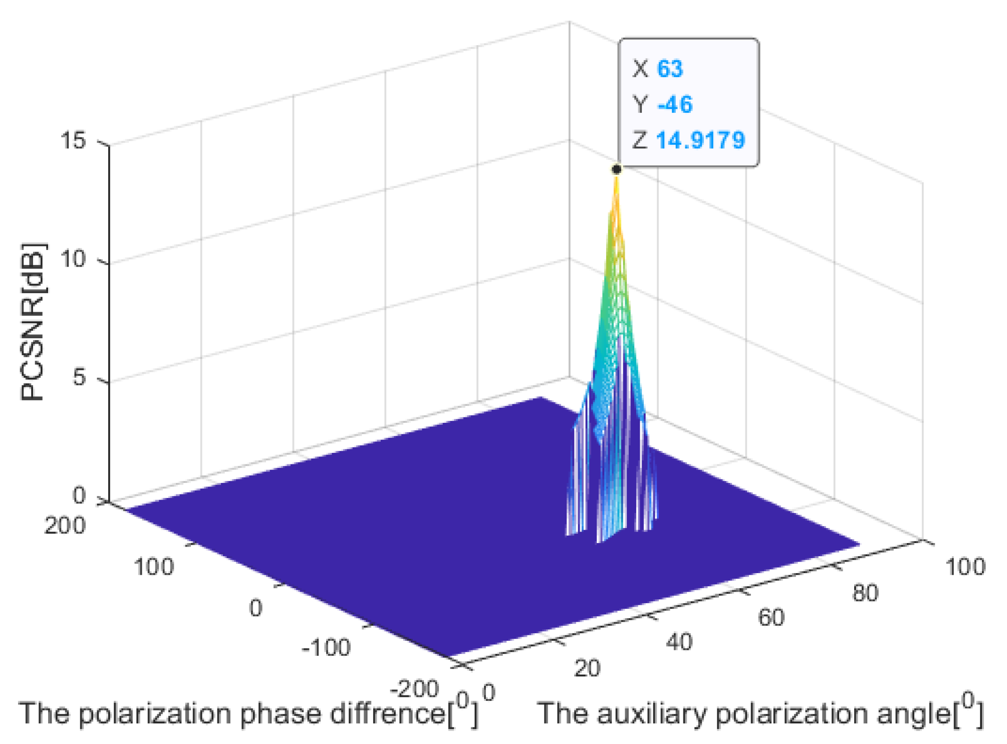
Radar transmits horizontal polarization and uses a crossed dipole as receiving antenna: $A_0=2$, $f_c=1.2\times {10}^9$, $T=2.5\times {10}^{-5}$, $k_c=1.6\times {10}^{12}$, the scattering matrix $\mathbf{S}=[1.20.4j;0.8j1.1]$. For the jamming interference between the current pulse, its polarization information is $({\gamma }_j={63}^{\circ },{\eta }_j={46}^{\circ })$, its ISR is 30 dB, and its frequency is $1.22\times {10}^9$.

With the continuous change of VPA $(\gamma ,\eta )$, the simulation results of the PCSNR are presented in Figure 1. Observing Figure 1, we can see that the PCSNR is at a maximum value at $(\gamma ={63}^{\circ },\eta =-{46}^{\circ })$. As $(\gamma ,\eta )$ changes to both ends, the PCSNR decreases sharply; thus, $(\gamma ={\gamma }_j,\eta =-{\eta }_j)$ is the maximum point. In summary, for signals containing both jamming interference and the target, the PCSNR is the largest when the parameter of VPA corresponds to the polarization of jamming interference; that is, $\gamma ={\gamma }_j$ and $\eta =-{\eta }_j$. Therefore, the proof of Theorem 2 is completed. □

3.3. Two-Dimensional Golden Section Method

For the signals containing both interference and target, it can be known that the PCSNR at $(\gamma ={\gamma }_j,\eta =-{\eta }_j)$ is the maximum point. Observing Equation (17), it is difficult to find the maximum point mathematically, so the numerical method is considered. If the accuracy of the polarization estimation is requested within $1^{\circ }$, it needs calculating $360\times 90=32,400$ times by traversing $(0^{\circ }\le \gamma \le {90}^{\circ },-{180}^{\circ }\le \eta \le {180}^{\circ })$. In order to speed up the calculation process, this subsection proposes the TDGSM to estimate the parameters of interference.

Based on Theorems 1 and 2, the estimation of interference can be described as a mathematical question; i.e., the PCSNR at $(\gamma ={\gamma }_j,\eta =-{\eta }_j)$ is unchanged and maximal, which is in accordance with the two-dimensional convex function. For the two-dimensional convex function in Figure 1, we propose the TDGSM, which can quickly search for the optimal solution in the interval. Its mathematical model is

$$\begin{array}{c}\underset{\left(\gamma ,\eta \right)\in D}{max}{f}_{PCSNR}\left(\gamma ,\eta \right)\hfill \\ sub.D=\left\{\left(\gamma ,\eta \right)|0^0\le \gamma \le {90}^0,-{180}^0\le \eta \le {180}^0\right\}\hfill \end{array},$$

(18)

where $f_{PCSNR}(\gamma ,\eta )$ is the PCSNR of the signal under VPA with the parameter of $(\gamma ,\eta )$. With a parameter of $\left(\gamma ,\eta \right)$, we can obtain the signal after down-conversion and pulse compression with Equation (17); i.e., $S_{VP{A}_j-pulse}\left(t\right)$. If the peak amplitude of $S_{VP{A}_j-pulse}\left(t\right)$ is $F_{peak}$ and the strongest side lobe is $F_{side}$, the $f_{PCSNR}(\gamma ,\eta )$ is given; i.e., $f_{PCSNR}(\gamma ,\eta )=F_{peak}/F_{side}$.

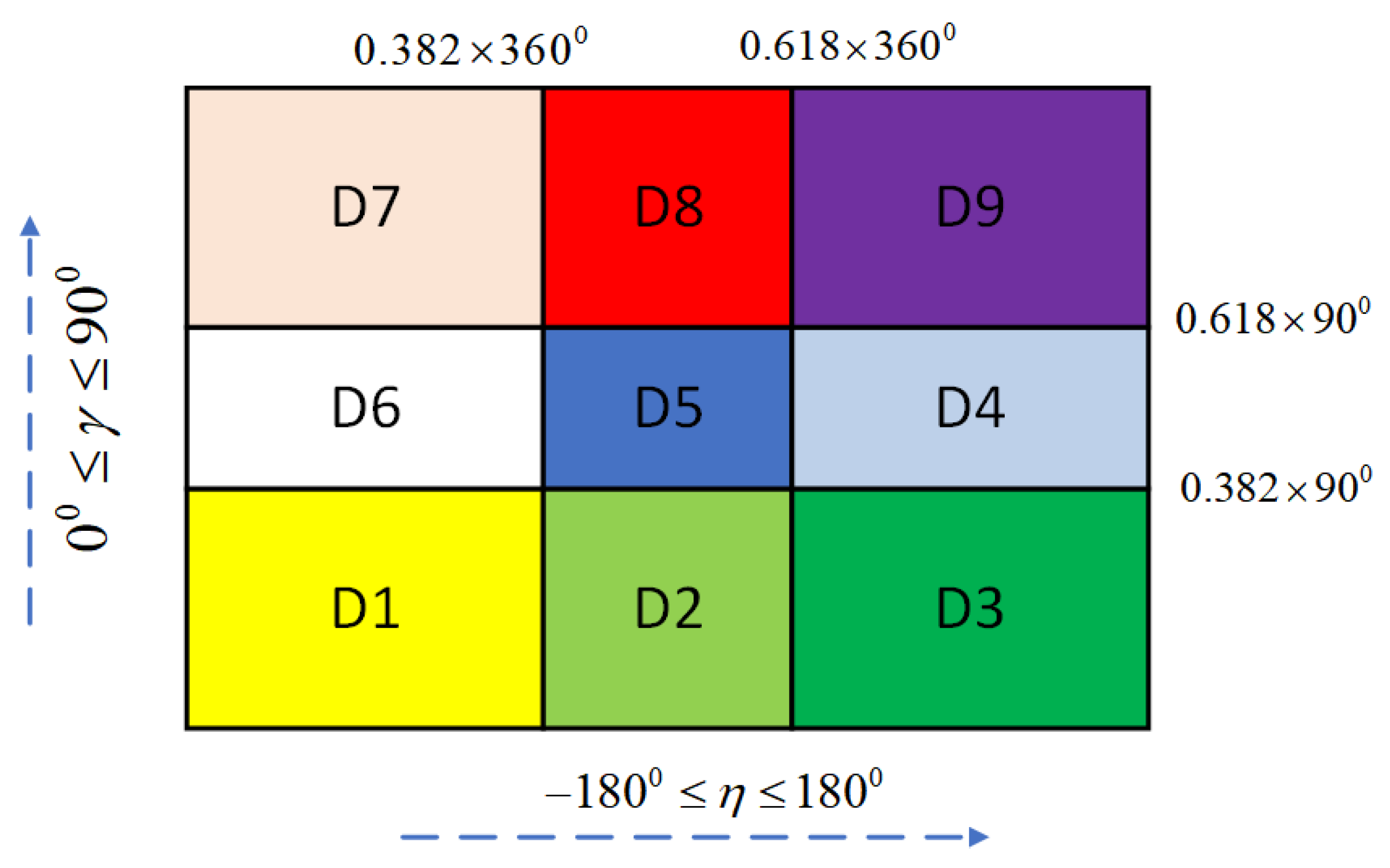
In the area of D, the vertical and horizontal directions are divided by 0.382 and 0.618, respectively, thus generating nine smaller areas, as shown in Figure 2. Subsequently, we calculate the PCSNR of every area’s center and select the area where the PCSNR is maximum in nine areas. Then, the selected area is re-divided into nine areas and the above process is iterated until the diameter of the area is smaller than the required accuracy. The steps of the TDGSM are as follows.

• Randomly select a point $({\gamma }^1,{\eta }^1)$ in the area of D; calculate $f_{PCSNR}^{*}=f_{PCSNR}({\gamma }^1,{\eta }^1)$ and $k=1$.
• Let the minimum be ${\gamma }_{min1}=0^{\circ }$ and maximum be ${\gamma }_{max1}={90}^{\circ }$ for the interval, The two golden section points of $\gamma$ are

  $$\begin{array}{c}{\gamma }_{{\beta }_1}=0.382({\gamma }_{max1}-{\gamma }_{min1})+{\gamma }_{min1}\hfill \\ {\gamma }_{{\phi }_1}=0.618({\gamma }_{max1}-{\gamma }_{min1})+{\gamma }_{min1}\hfill \end{array}.$$

  (19)
  Let the minimum be ${\eta }_{min1}=-{180}^{\circ }$ and maximum be ${\eta }_{max1}={180}^{\circ }$ for the interval. The two golden section points of $\eta$ are

  $$\begin{array}{c}{\eta }_{{\beta }_1}=0.382({\eta }_{max1}-{\eta }_{min1})+{\eta }_{min1}\hfill \\ {\eta }_{{\phi }_1}=0.618({\eta }_{max1}-{\eta }_{min1})+{\eta }_{min1}\hfill \end{array}.$$

  (20)
  The area of D is divided into nine areas by ${\gamma }_{{\beta }_1}$, ${\gamma }_{{\phi }_1}$, ${\eta }_{{\beta }_1}$, and ${\eta }_{{\phi }_1}$; i.e., $D_i^1$, $i=1,...,9$, as shown in Figure 2. The center of $D_i^1$ is $({\gamma }_i^1,{\eta }_i^1)$, the diameter of $D_i^1$ is $d_i^1$, and $k=1$.
• If $\underset{i=1,...,9}{min}{d}_i^k\le d_0$ where $d_0$ is the required accuracy, stop the calculation and go to Step 6; otherwise, go to Step 4.
• Calculate the PCSNR of nine golden section points. If the maximum of $f_{PCSNR}({\gamma }_i^k,{\eta }_i^k)$ is greater than $f_{PCSNR}^{*}$, i.e., $i=j$, let $({\gamma }_{mink+1},{\gamma }_{maxk+1})$ and $({\eta }_{mink+1},{\eta }_{maxk+1})$ is in the range of $D_j^k$, $({\gamma }^{k+1},{\eta }^{k+1})=({\gamma }_j^k,{\eta }_j^k)$, $f_{PCSNR}^{*}=f_{PCSNR}({\gamma }_j^k,{\eta }_j^k)$, go to Step 5; otherwise, go to Step 6.
• Let $k=k+1$, return to Step 2.
• The estimated parameter is $({\gamma }^k,{\eta }^k)$ and the iteration is stopped.

Through the TDGSM, the parameter estimation of interference can be completed in an iterative loop. If the estimation accuracy of the polarization parameters is controlled within $1^{\circ }$, the iteration amount ∑ is in the range of $({\sum }_{min},{\sum }_{max})$, as shown in Equation (21).

$$\begin{array}{c}{360}^{\circ }\times 0.{382}^{{\sum }_{max}}\le 1^{\circ }\hfill \\ {360}^{\circ }\times 0.{236}^{{\sum }_{min}}\le 1^{\circ }\hfill \end{array},$$

(21)

where ${\sum }_{max}$ denotes that the selected area always belongs to $D_1$, $D_3$, $D_7$, and $D_9$ in Figure 2; ${\sum }_{min}$ represents that the selected area always belongs to $D_5$.

From Equation (21), the range of the iteration amount is $5\le \sum \le 7$; thus, the total calculation is in the range of $(45,63)$. Compared to $360\times 90=32,400$ times by traversing $(0^{\circ }\le \gamma \le {90}^{\circ },-{180}^{\circ }\le \eta \le {180}^{\circ })$, the TDGSM in this paper significantly reduces the amount of calculation. Subsequently, we further analyze the characteristic of TDGSM as follows.

Theorem 3.

The estimation of the TDGSM is not only convergent, but also globally optimal.

Proof of Theorem 3.

Initially, we randomly select a point $({\gamma }^1,{\eta }^1)$ in the area of D and calculate $f_{PCSNR}^{*}=f_{PCSNR}({\gamma }^1,{\eta }^1)$. Then, the maximum PCSNR $f_{PCSNR}({\gamma }_i^k,{\eta }_i^k)$ in nine areas is compared with $f_{PCSNR}^{*}$ in each iteration. If $f_{PCSNR}({\gamma }_i^k,{\eta }_i^k)$ is greater than $f_{PCSNR}^{*}$, we replace the $f_{PCSNR}({\gamma }_i^{k+1},{\eta }_i^{k+1})$ and $({\gamma }^{k+1},{\eta }^{k+1})$, so that $f_{PCSNR}({\gamma }_i^{k+1},{\eta }_i^{k+1})$ is greater than $f_{PCSNR}^{*}$. Based on the above conclusion, the estimation of the TDGSM must converge; therefore, there is an upper bound $f_{PCSNR}^{*}$.

Assuming that the estimation of the TDGSM is not globally optimal, there is a point $({\gamma }^0,{\eta }^0)$ in D where $f_{PCSNR}({\gamma }^0,{\eta }^0)$ is greater than $f_{PCSNR}^{*}$. Based on the continuity function, there must be a field U near this point $({\gamma }^0,{\eta }^0)$ to satisfy the requirement that all points in the field be greater than $f_{PCSNR}^{*}$. However, note that in the iterative process, the diameters of areas, i.e., $d_1,..,d_9$, will tend towards 0, so there must be an area that falls completely within the field U. Since all PCSNRs in the area are less than $f_{PCSNR}^{*}$, this conclusion contradicts the above result that all points in the field U are greater than $f_{PCSNR}^{*}$. To sum up, the above assumption does not hold, so the estimation of TDGSM is globally optimal, thus completing the proof of Theorem 3. □

4. Performance Analysis

In this section, three aspects—robustness, complexity, and applicability—are analyzed to investigate the performance of the presented method.

4.1. Robustness Analysis of Different SNRs

Because noise can create polarization measurement errors, we discuss the influence of noise on the presented method, comparing it with that of the ISMA in Reference [58]. In order to obtain a better robustness analysis, we explain this in the following example.

Example 2.

Radar transmits horizontal polarization and uses a crossed dipole as receiving antenna: $A_0=2$, $f_c=1.2\times {10}^9$, $T=2.5\times {10}^{-5}$, $k_c=1.6\times {10}^{12}$, scattering matrix $\mathbf{S}=[1.20.4j;0.8j1.1]$. For the jamming interference between current pulses, the polarization parameters are $({\gamma }_j={32}^{\circ },{\eta }_j={63}^{\circ })$, the amplitude is ${10}^3$, $f_j=1.22\times {10}^9$, and the signal-to-interference ratio (SIR) is −40 dB. For the noise, we assume that the horizontal and vertical receiving antennas obey the zero-mean Gaussian distribution.

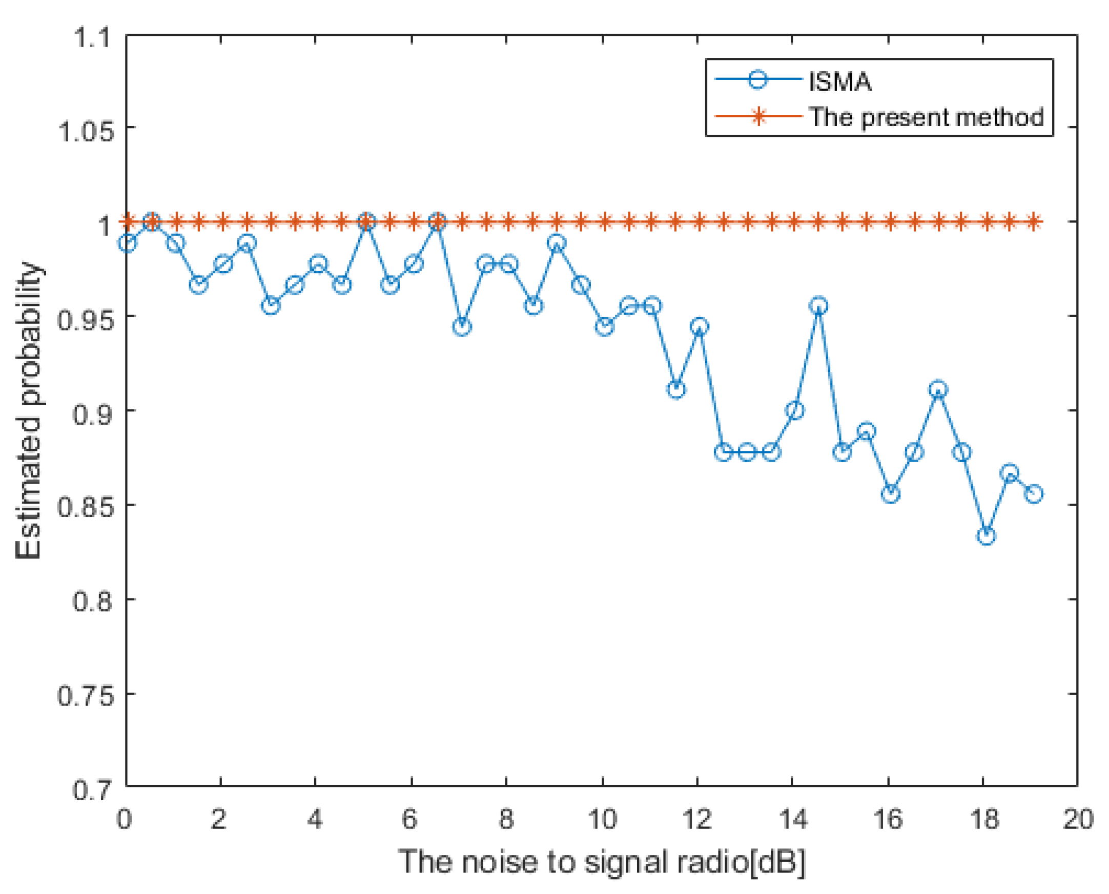
For the signals that contain target, jamming interference, and noise simultaneously, we let the signal-to-noise ratio (SNR) change in $[-20\mathrm{dB},0\mathrm{dB}]$. For different SNRs, we randomly select $({\gamma }_j,{\eta }_j)$ in their range and perform a Monte Carlo simulation 100 times. Figure 3 displays the correct rate of ISMA and the presented method under the assumption that the estimation of $({\gamma }_j,{\eta }_j)$ is the correct estimate when the estimated error satisfies $(\Delta \gamma \le 2^{\circ },\Delta \eta \le 2^{\circ })$. Observing Figure 3, we can see that the correct rate of ISMA decreases if the SNR decreases, whereas the correct rate of the presented method remains unchanged. Especially when the noise is large (e.g., the SNR is less than −12 dB), the estimated probability of the presented method is much better than ISMA. There is a main reason for this phenomenon; i.e., ISMA processes the pre-pulse compression data, while the presented method processes the post-pulse compression data. When comparing the target with the jamming interference after the pulse compression, the influence of the SNR in $[-20\mathrm{dB},0\mathrm{dB}]$ is extremely small. Therefore, the presented method has better robustness when compared with ISMA.

4.2. Complexity Analysis

When comparing with the signal processing of radar, the presented method in this paper only adds to the operation of VPA, as exhibited below in Equation (22).

$$s_{VPA}\left(t\right)=\left[sin\gamma -cos\gamma e^{j\eta }\right]\left[\begin{array}{c}{E}_h\hfill \\ E_v\hfill \end{array}\right].$$

(22)

After the VPA, the number of compared operations in the range of $(45,63)$ are carried out on the PCSNR. Because the presented method needs to repeat the 45 to 63 calculations, the computation is greater than in ISMA. On the other hand, the presented method in this paper only processes echoes within the distance window, and the signal length is much shorter than the original echoes in ISMA, which can simplify the calculation. We tested the time requirements of the two methods on the same device, with a computational platform with a $i7-10510U$ CPU quad-core and 16 Gb of memory. The CPU time for ISMA is 0.0040 s, while the CPU time for the presented method in this paper is 0.0128 s, which is about 3.2 times that of ISMA.

4.3. Applicability Analysis

In the proof of Theorem 2, we assume that the amplitude of jamming interference is much higher than that of target echo after pulse compression. For the signals containing both jamming interference and the target, the PCSNR is the largest when the parameter of VPA correspond to the polarization of jamming interference; that is, $\gamma ={\gamma }_j$ and $\eta =-{\eta }_j$. However, due to the influence of interference in other received parameters, the main lobe of the target may rise or the side lobe may decrease, which would lead to that the PCSNR of target increasing. Therefore, the PCSNR of the target echo with VPA of $\gamma ={\gamma }_j$ and $\eta =-{\eta }_j$ may no longer be the maximum value when the amplitude of the jamming interference gradually decreases. To further explain this phenomenon, we also give an example in the following, the parameters of which are the same as in Example 1, except for the difference in the amplitude of jamming interference.

Example 3.

Radar transmits horizontal polarization and uses a crossed dipole as receiving antenna: $A_0=2$, $f_c=1.2\times {10}^9$, $T=2.5\times {10}^{-5}$, $k_c=1.6\times {10}^{12}$, the scattering matrix $\mathbf{S}=[1.20.4j;0.8j1.1]$. For the jamming interference between the current pulse, polarization is $({\gamma }_j={35}^{\circ },{\eta }_j={75}^{\circ })$ and amplitude is 2, $f_j=1.22\times {10}^9$.

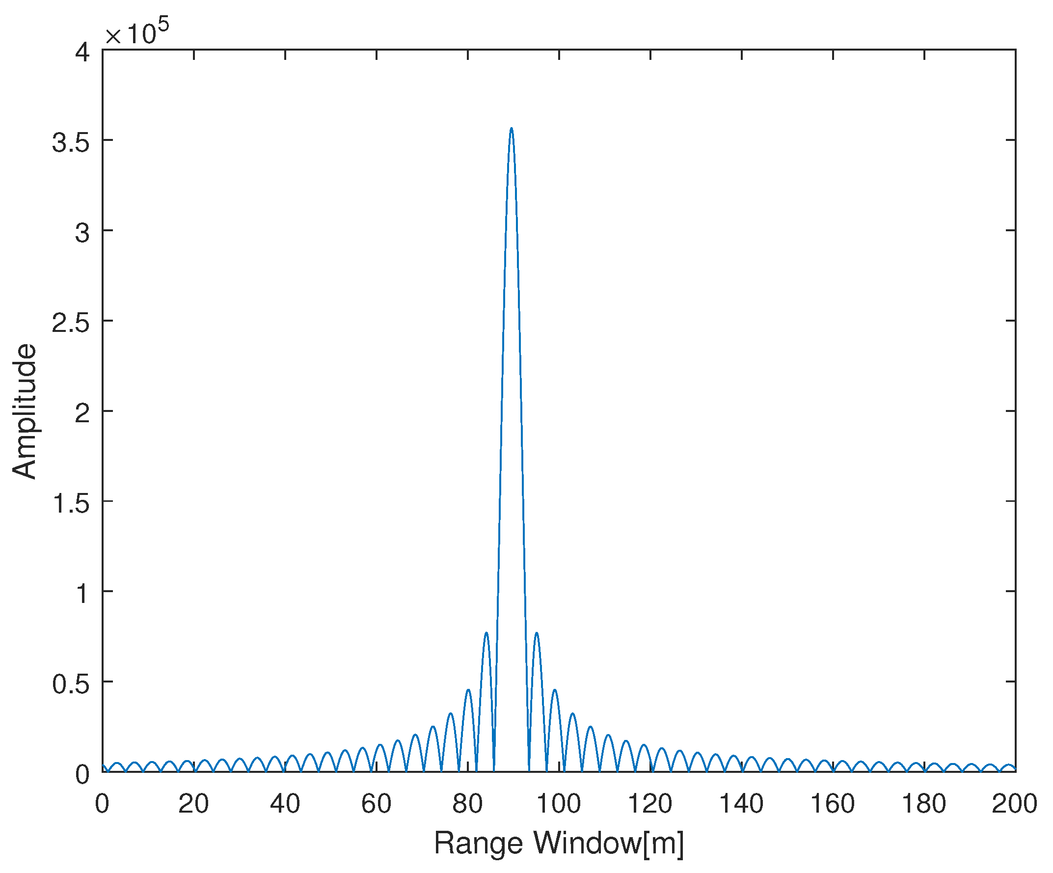
When the parameter of VPA corresponds to the polarization of jamming interference, i.e., $(\gamma ={\gamma }_j,\eta =-{\eta }_j)$, the target echoes after pulse compression are similar to those in Figure 4. In this case, the PCSNR is 13.29 dB. However, when the parameter of VPA is $(\gamma ={39}^{\circ },\eta =-{78}^{\circ })$, the PCSNR is 14.34 dB in the nonideal VPA. The target echoes after pulse compression are displayed in Figure 5. Therefore, the PCSNR of target echoes is no longer a maximum value under the interference condition, which is affected by different ISRs. In order to further analyze the minimum requirement for ISR contained in Theorem 2, Monte Carlo simulation was performed for different ISRs. We give another example to explain this point.

Example 4.

Radar transmits horizontal polarization and uses a crossed dipole as receiving antenna:$A_0=2$, $f_c=1.2\times {10}^9$, $T=2.5\times {10}^{-5}$, $k_c=1.6\times {10}^{12}$, the scattering matrix$\mathbf{S}=[1.20.4j;0.8j1.1]$. For the jamming interference between the current pulse,$f_J=1.22\times {10}^9$.

For different ISRs, we randomly select $({\gamma }_j,{\eta }_j)$ 100 times in the range $(0^{\circ }\le {\gamma }_j\le {90}^{\circ },-{180}^{\circ }\le {\eta }_j\le {180}^{\circ })$, and estimate its polarization by TDGSM. By calculating the estimated probability under different ISRs, we can obtain the minimum requirement for ISR in Theorem 2, as displayed in Figure 6. Combining Example 4 with Figure 6, the presented method can be affected by the amplitude of jamming interference. When the amplitude of the interference signal makes Theorem 2 hold, it is suitable for the method presented in this paper. However, when the jamming interference energy is low, the estimation error of the presented method will increase. From a numerical analysis in Figure 6, we see that when the ISR is greater than 28.75 dB, the estimated probability of the presented method is higher than 0.99. As ISR increases, the estimated probability approaches 1. If Equations (12) and (13) are directly performed on the received signal, the target can be detected when the ISR is in the range of [0 dB, 15.4 dB]. In summary, the presented method in this paper is applicable when the ISR is in the range of [0 dB, 15.4 dB] and [28.75 dB, ∞ dB].

5. Simulation

The Section 4 analyzes the presented method from three aspects: robustness, complexity, and applicability. In this section, the numerical results are analyzed for specific cases where the target belongs to the distributed type and the polarization of the interference is changing.

Example 5.

The parameters of radar, target, interference, and noise are as follows.

• Radar transmits horizontal polarization and uses a crossed dipole as receiving antenna. Its signal amplitude is $A_0=2$, carrier frequency $f_c=1.2\times {10}^9$, pulse width $T=2.5\times {10}^{-5}$, bandwidth $B=40\times {10}^6$, pulse repetition period $PRI=2\times {10}^3$, and pulse number $N=16$.
• The distance between the distributed target, the window’s center, and target’s relative RCS are [90 m 2; 95 m 1.2; 105 m, 1]. The speed of light $c=3\times {10}^8$, and the scattering matrix $\mathbf{S}=[1.20.4j;0.8j1.1]$.
• The jammer’s carrier frequency $f_J=1.2\times {10}^9$, ISR = 34 dB. The polarization parameter of the jammer is changing between different pulses. In order to observe the accuracy of estimation in different pulses, we fix the auxiliary polarization angle ${\gamma }_j={36}^{\circ }$ and randomly select the polarization phase difference ${\eta }_j$ in different pulses, as exhibited in

  Table 1. The polarization phase difference of interference in different pulses.

  Num.	Polarization Phase Difference	Num.	Polarization Phase Difference	Num.	Polarization Phase Difference
  1	${22}^{\circ }$	7	${77}^{\circ }$	13	${40}^{\circ }$
  2	${54}^{\circ }$	8	${27}^{\circ }$	14	${56}^{\circ }$
  3	${52}^{\circ }$	9	${47}^{\circ }$	15	${71}^{\circ }$
  4	${13}^{\circ }$	10	${18}^{\circ }$	16	${77}^{\circ }$
  5	${10}^{\circ }$	11	${60}^{\circ }$
  6	${40}^{\circ }$	12	${20}^{\circ }$

  .
• Assume that the noise in the crossed dipole follows the Gaussian distribution and $SNR$ = 0 dB.

Taking the 16th pulse containing target, interference, and noise as an example, we perform down-conversion, filtering, and pulse compression on the horizontal received signal, as shown in Figure 7. We can see that the target signal after pulse compression is very weak, due to the influence of jamming interference under the same frequency and the main lobe as radar, which seriously affect the subsequent target detection.

Subsequently, we utilize the presented method to continuously estimate the parameters of interference between 16 pulses, which is shown in Figure 8. Observing Figure 8, the presented method can estimate the parameters well, and the accuracy is within 1${}^{\circ }$ when the polarization of interference is continuously variable and randomly selected. Taking the 16th pulse as an example, the pulse compression result of VPA with the parameters $({36}^{\circ },-{77}^{\circ })$ s shown in Figure 9 when simply performing interference suppression with conjugate reception polarization. In Figure 9, we can see that the target’s PCSNR is 12.74 dB, which is higher than that of the horizontal received signal in Figure 7 after the accurately estimation of interference and conjugate polarization reception.

We then compared the presented method and ISMA in terms of estimation accuracy, which also further verified the conclusion in Section 4.

Example 6.

The simulation parameters are the same as those in Example 5, i.e., radar, target, and interference. We compare the estimation accuracy of both the methods under different SNRs—$SN{R}_1=-10$dB,$SN{R}_2=-20$dB—as shown in Figure 10 and Figure 11.

Observing Figure 10 and Figure 11, we can find that as SNR decreases, the error of ISMA increases. In addition, the presented method remains unchanged within the SNR of [−20 dB, 0 dB], which is consistent with the results in Section 4.1.

Example 7.

The simulation parameters are the same as those in Example 5, i.e., radar, target, and interference. We compare the estimation accuracy of both the methods under different ISRs—$IS{R}_1=28$dB,$JS{R}_1=40$dB—as shown in Figure 12 and Figure 13.

Observing Figure 10, Figure 12, and Figure 13, we can find that the error of ISMA increases as the ISR decreases. When the ISR is greater than 28 dB, the estimated probability of the presented method is higher than 0.99, which verifies the results in Section 4.3.

6. Conclusions

For signals containing target, interference, and noise, this paper proposes a novel synchronous estimation method for interference with different polarizations. First, we introduced the polarization invariant, i.e., the PCSNR. Then, an estimation method was proposed based on two theorems of the polarization invariant. Subsequently, we proposed the TDGSM to further optimize this method with minimum calculation, and proved that the method presented in this paper is convergent and globally optimal. Finally, the presented method was analyzed in terms of three aspects: robustness, complexity, and applicability.

References

- Yu, H.L.; Liu, N.; Zhang, L.R. An interference suppression method for multistatic radar based on noise subspace projection. IEEE Sensors J. 2020, 15, 8797–8805. [Google Scholar] [CrossRef]
- Chen, G.; Wang, J.; Zuo, L. Two-stage clutter and interference cancellation method in passive bistatic radar. IET Signal Process. 2020, 6, 342–351. [Google Scholar]
- Ge, M.G.; Cui, G.L.; Yu, X.X. Main lobe jamming suppression via blind source separation sparse signal recovery with subarray configuration. IET Radar Sonar Navig. 2020, 3, 431–438. [Google Scholar] [CrossRef]
- Liu, Z.Y.; Kong, Y.G.; Zhang, X. Vital sign extraction in the presence of radar mutual interference. IEEE Signal Process. Lett. 2020, 27, 1745–1749. [Google Scholar] [CrossRef]
- Sinclair, G. The transmission and reception of elliptically polarized waves. Proc. IRE 1950, 2, 148–151. [Google Scholar] [CrossRef]
- Kennaugh, E.M. Polarization Properties of Radar Reflections. Electronic Thesis, Ohio State University, Columbus, UK, 1952. [Google Scholar]
- Huynen, J.R. Phenomenological theory of radar targets. Ph.D. Thesis, Technical University, Delft, The Netherland, 1970. [Google Scholar]
- Zhe, G.; Deng, H.; Himed, B. Adaptive radar beamforming for interference mitigation in radar-wireless spectrum sharing. IEEE Signal Process. Lett. 2014, 4, 484–488. [Google Scholar]
- Zhe, X.; Chen, B.; Yang, M. Transmitter polarization optimization with polarimetric MIMO radar for mainlobe interference suppression. Digital Signal Process. 2017, 65, 19–26. [Google Scholar]
- Zhang, X.; Cao, D.; Xu, L.L. Joint polarization and frequency diversity for deceptive jamming suppression in MIMO radar. IET Radar Sonar Navig. 2019, 13, 263–271. [Google Scholar] [CrossRef]
- Mao, X.P.; Jun, L.A. Null phase-shift polarization filtering for high-frequency radar. IEEE Trans. Aerosp. Electron. Syst. 2007, 4, 1397–1408. [Google Scholar] [CrossRef]
- Jun, L.A.; Mao, X.P.; Deng, W.B. Oblique projection polarization filtering and its performance in high frequency surface wave radar. In Proceedings of the International Conference on Microwave and Millimeter Wave Technology IEEE, Chengdu, China, 8–11 May 2010; pp. 1618–1621. [Google Scholar]
- Mao, X.P.; Jun, L.A.; Hou, H.J. Oblique projection polarization filtering for interference suppression in high-frequency surface wave radar. IET Radar Sonar Navig. 2012, 2, 71–80. [Google Scholar] [CrossRef]
- Hong, H.; Mao, X.P.; Hu, C. A multi-domain collaborative filter for HFSWR based on oblique projection. In Proceedings of the IEEE National Radar Conference Proceedings, Atlanta, GA, USA, 7 May 2012; pp. 907–912. [Google Scholar]
- Zhe, X.; Chen, B.; Yang, M. Transmitter/receiver polarization optimisation based on oblique projection filtering for mainlobe interference suppression in polarimetric multiple-input–multiple-output radar. IET Radar Sonar Navig. 2018, 1, 137–144. [Google Scholar]
- Shi, L.F. Study with the Suppression of Interference Radar Polarization Information. Ph.D. Thesis, University of National Defense, Changsha, China, 2007. [Google Scholar]
- Chang, Y.L.; Wong, X.S.; Li, Y.Z. Polarization filter realization method for multiple noise FM interference. Aerosp. Electron. Warf. 2010, 3, 39–42. [Google Scholar]
- Ren, B.; Shi, L.F.; Wang, H.J. Investigation on of polarization filtering scheme to suppress GSM interference in radar main beam. J. Electron. Inf. Technol. 2014, 2, 459–464. [Google Scholar]
- Dai, H.X.; Li, Y.Z.; Wang, X.S. Interference cancellation and polarization suppression technology based on monopulse radar. Radar Sci. Technol. 2010, 5, 431–437. [Google Scholar]
- Dai, H.Y.; Huan, Z.; Lei, H. Interference cancellation and polarization suppression technology based on the pattern difference between sum-and-difference beams in mono-pulse radar. In Proceedings of the Radar Conference IEEE, Lille, France, 13 October 2015; pp. 1–6. [Google Scholar]
- Ma, J.Z.; Shi, L.F.; Li, Y.Z. Angle estimation of extended targets in main-lobe interference with polarization filtering. IEEE Trans. Aerosp. Electron. Syst. 2017, 1, 169–189. [Google Scholar] [CrossRef]
- Ma, J.Z.; Shi, L.F.; Xiao, S.P. Mitigation of cross-eye jamming using a dual-polarization array. J. Syst. Eng. Electron. 2018, 3, 491–498. [Google Scholar]
- Li, J.L.; Luo, J.; Chang, Y.L. Virtual polarization receiver based on the spatial polarization characteristics of antenna. Chin. J. Radio Sci. 2009, 3, 389–393. [Google Scholar]
- Dai, H.Y.; Wang, X.S.; Li, Y.Z. Main-lobe jamming suppression method of using spatial polarization characteristics of antennas. IEEE Trans. Aerosp. Electron. Syst. 2012, 3, 2167–2179. [Google Scholar] [CrossRef]
- Tohid, T.; Norouzi, Y.; Rajabi, A. A novel method for interference cancellation using polarization filter. In Proceedings of the IEEE Microwaves, Radar and Remote Sensing Symposium, Kiev, Ukraine, 29–31 August 2017; pp. 233–238. [Google Scholar]
- He, J.; Wang, Y.; Shu, T.; Truong, T.K. Polarization, Angle, and Delay Estimation For Tri-Polarized Systems in Multipath Environments. IEEE Trans. Wirel. Commun. 2022. [Google Scholar] [CrossRef]
- Xie, L.; He, Z.; Tong, J.; Liu, T.; Li, J.; Xi, J. Regularized Covariance Estimation for Polarization Radar Detection in Compound Gaussian Sea Clutter. IEEE Trans. Geosci. Remote Sens. 2022. [Google Scholar] [CrossRef]
- Nehorai, A.; Paldi, E. Superresolution compact array radiolocation technology (SuperCART) project. In Proceedings of the Conference Record of the Twenty-Fifth Asilomar Conference on Signals, Systems and Computers, Pacific Grove, CA, USA, 4–6 November 1991; pp. 566–572. [Google Scholar]
- Nehorai, A.; Paldi, E. Vector-sensor array processing for electromagnetic source localization. IEEE Trans. Signal Process. 1994, 2, 376–398. [Google Scholar] [CrossRef]
- Hochwald, B.; Nehorai, A. Polarimetric modeling and parameter estimation with applications to remote sensing. IEEE Trans. Signal Process. 1995, 8, 1923–1935. [Google Scholar] [CrossRef]
- Hochwald, B.; Nehorai, A. Identifiability in array processing models with vector-sensor applications. IEEE Trans. Signal Process. 1996, 1, 83–95. [Google Scholar] [CrossRef]
- Tan, K.C.; Ho, K.C.; Nehorai, A. Uniqueness study of measurements obtainable with arrays of electromagnetic vector sensors. IEEE Trans. Signal Process. 1996, 4, 1036–1039. [Google Scholar]
- Nehorai, A.; Ho, K.C.; Tan, B.T.G. Minimum-noise-variance beamformer with an electromagnetic vector sensor. IEEE Trans. Signal Process. 1999, 3, 601–618. [Google Scholar] [CrossRef]
- Ho, K.C.; Tan, K.C.; Tan, B.T.G. Estimation of directions of-arrival of partially polarized signals with electromagnetic vector sensors. In Proceedings of the IEEE International Conference on Acoustics, Speech, and Signal Processing Conference Proceedings, Atlanta, CA, USA, 9 May 1996. [Google Scholar]
- Ho, K.C.; Tan, K.C.; Tan, B.T.G. Efficient method for estimating directions-of-arrival of partially polarized signals with electromagnetic vector sensors. IEEE Trans. Signal Process. 1997, 10, 2485–2498. [Google Scholar]
- Ho, K.C.; Tan, K.C.; Nehorai, A. Estimating directions of arrival of completely and incompletely polarized signals with electromagnetic vector sensors. IEEE Trans. Signal Process. 1999, 10, 2845–2852. [Google Scholar] [CrossRef]
- Zoltowski, M.D.; Wong, K.T. Extended-aperture spatial diversity and polarizational diversity using a sparse array of electric dipoles or magnetic loops. In Proceedings of the IEEE 47th Vehicular Technology Conference. Technology in Motion, Phoenix, AZ, USA, 4–7 May 1997. [Google Scholar]
- Ko, C.C.; Zhang, J.; Nehorai, A. Separation and tracking of multiple broadband sources with one electromagnetic vector sensor. IEEE Trans. Aerosp. Electron. Syst. 2002, 2, 1109–1116. [Google Scholar] [CrossRef]
- Wong, K.T.; Zoltowski, M.D. Self-initiating MUSIC-based direction finding and polarization estimation in spatio-polarizational beamspace. IEEE Trans. Antennas Propag. 2000, 8, 1235–1245. [Google Scholar]
- Li, J. Direction and polarization estimation using arrays with small loops and short dipoles. IEEE Trans. Antennas Propag. 1993, 3, 379–387. [Google Scholar] [CrossRef]
- Li, J.; Compton, R.T. Angle and polarization estimation using ESPRIT with a polarization sensitive array. IEEE Trans. Antennas Propag. 1991, 9, 1376–1383. [Google Scholar] [CrossRef]
- Li, J.; Compton, R.T. Angle estimation using a polarization sensitive array. IEEE Trans. Antennas Propag. 1991, 10, 1539–1543. [Google Scholar] [CrossRef]
- Li, J.; Compton, R.T. Two dimensional angle and polarization estimation using the ESPRIT algorithm. IEEE Trans. Antennas Propag. 1992, 5, 550–555. [Google Scholar] [CrossRef]
- Li, J.; Compton, R.T. Angle and polarization estimation in a coherent signal environment. IEEE Trans. Aerosp. Electron. Syst. 1993, 3, 706–716. [Google Scholar] [CrossRef]
- Qiu, S.; Sheng, W.; Ma, X.; Kirubarajan, T. A Maximum Likelihood Method for Joint DOA and Polarization Estimation Based on Manifold Separation. IEEE Trans. Aerosp. Electron. Syst. 2021, 4, 2481–2500. [Google Scholar] [CrossRef]
- Li, J.; Stoica, P. Efficient parameter estimation of partially polarized electromagnetic waves. IEEE Trans. Signal Process. 1994, 11, 3114–3125. [Google Scholar] [CrossRef]
- Li, J. On polarization estimation using a crossed-dipole array. IEEE Trans. Signal Process. 1994, 2, 977–980. [Google Scholar] [CrossRef]
- Li, J.; Stoica, P.; Zheng, D. Efficient direction and polarization estimation with a COLD array. IEEE Trans. Antennas Propag. 1996, 4, 539–547. [Google Scholar] [CrossRef]
- Zoltowski, M.D.; Wong, K.T. Closed-form eigenstructure-based direction finding using arbitrary but identical subarrays on a sparse uniform Cartesian array grid. IEEE Trans. Signal Process. 2000, 8, 2205–2210. [Google Scholar] [CrossRef] [Green Version]
- Zoltowski, M.D.; Wong, K.T. ESPRIT-based 2-D direction finding with a sparse uniform array of electromagnetic vector-senors. IEEE Trans. Signal Process. 2000, 8, 2195–2204. [Google Scholar] [CrossRef]
- Wong, K.T.; Zoltowski, M.D. Closed-form direction finding and polarization estimation with arbitrarily spaced electromagnetic vector-sensors at unknown locations. IEEE Trans. Antennas Propag. 2000, 5, 671–681. [Google Scholar] [CrossRef] [Green Version]
- Wong, K.T. Direction finding/polarization estimation–dipole and/or loop triad(s). IEEE Trans. Aerosp. Electron. Syst. 2001, 2, 679–684. [Google Scholar]
- Wong, K.T.; Yuan, X. Vector cross-product direction-finding with an electromagnetic vector-sensor of six orthogonally oriented but spatially noncollocating dipoles/loops. IEEE Trans. Signal Process. 2011, 1, 160–171, Erratum in IEEE Trans. Signal Process. 2014, 4, 1028–1030. [Google Scholar] [CrossRef]
- Wong, K.T.; Li, L.S.; Zoltowski, M.D. Root-MUSIC-based direction-finding and polarization estimation using diversely polarized possibly collocated antennas. IEEE Trans. Wirel. Propag. Lett. 2004, 1, 129–132. [Google Scholar] [CrossRef]
- Comption, R.T. The tripole antenna: An adaptive array with full polarization flexibility. IEEE Trans. Antennas Propag. 1981, 6, 944–952. [Google Scholar] [CrossRef]
- Comption, R.T. The performance of a tripole adaptive array against cross-polarized jamming. IEEE Trans. Antennas Propag. 1983, 4, 682–685. [Google Scholar] [CrossRef]
- Yeung, C.K.A.; Wong, K.T. CRB: Sinusoid-sources estimation using collocated dipoles/loops. IEEE Trans. Aerosp. Electron. Syst. 2009, 1, 94–109. [Google Scholar] [CrossRef]
- Li, Y.Z.; Xiao, S.P.; Wang, X.S. Polarization cancellation method for self-defense suppression interference based on auxiliary antenna. In Radar Polarization Anti-jamming Technology; Li, Y.Z., Ed.; National Defense Industry Press: Beijing, China, 2010; pp. 151–160. [Google Scholar]
Figure 1.
PCSNR of signals under different received polarization.
Figure 2.
The divided areas in the TDGSM.
Figure 3.
Estimated probability of the two methods under different CSRs.
Figure 4.
PCSNR at an ideal VPA parameter.
Figure 5.
PCSNR at a nonideal VPA parameter.
Figure 6.
Estimated probability under different ISRs.
Figure 7.
Pulse compression results of the horizontal received signal.
Figure 8.
The estimation result of SPPEM.
Figure 9.
Pulse compression result received by conjugate polarization.
Figure 10.
The estimation of the two methods under 10 dB.
Figure 11.
The estimation of these two methods under 20 dB.
Figure 12.
The estimation of the two methods under = 28 dB.
Figure 13.
The estimation of these two methods under = 40 dB.