The Multisource Vegetation Inventory (MVI): A Satellite-Based Forest Inventory for the Northwest Territories Taiga Plains

Abstract

Sustainable forest management requires information on the spatial distribution, composition, and structure of forests. However, jurisdictions with large tracts of noncommercial forest, such as the Northwest Territories (NWT) of Canada, often lack detailed forest information across their land base. The goal of the Multisource Vegetation Inventory (MVI) project was to create a large area forest inventory (FI) map that could support strategic forest management in the NWT using optical, radar, and light detection and ranging (LiDAR) satellite remote sensing anchored on limited field plots and airborne LiDAR data. A new landcover map based on Landsat imagery was the first step to stratify forestland into broad forest types. A modelling chain linking FI plots to airborne and spaceborne LiDAR was then developed to circumvent the scarcity of field data in the region. The developed models allowed the estimation of forest attributes in thousands of surrogate FI plots corresponding to spaceborne LiDAR footprints distributed across the project area. The surrogate plots were used as a reference dataset for estimating each forest attribute in each 30 m forest cell within the project area. The estimation was based on the k-nearest neighbour (k-NN) algorithm, where the selection of the four most similar surrogate FI plots to each cell was based on satellite, topographic, and climatic data. Wall-to-wall 30 m raster maps of broad forest type, stand height, crown closure, stand volume, total volume, aboveground biomass, and stand age were created for a ~400,000 km² area, validated with independent data, and generalized into a polygon GIS layer resembling a traditional FI map. The MVI project showed that a reasonably accurate FI map for large, remote, predominantly non-inventoried boreal regions can be obtained at a low cost by combining limited field data with remote sensing data from multiple sources.

1. Introduction

A forest inventory (FI) provides information on the spatial distribution, composition, and structure of forest stands within a forested area [1,2]. Provincial and territorial FIs in Canada are based on photo interpretation of digital aerial photographs at a nominal scale of 1:20,000, which results in a map comprised of polygons ranging in size from a few to thousands of hectares [3]. Since the 2000s, these maps have been produced in a softcopy environment that enables the interpreter to visualize the imagery in a digital stereo-viewing (3D) system, digitize stand boundaries on-screen, and add attributes such as tree species composition, stand height, and crown closure to each delineated polygon and store them as a geographic information system (GIS) layer [4].

The Northwest Territories (NWT) has over 40 million hectares (Mha) of forests that are broadly distributed within 80 Mha of land, much of which is inaccessible. Conventional inventories have been undertaken since at least the 1970s, resulting in data of varying vintage and measurement standards across an extent of less than 10% of its forests. Even if they are assumed to be accurate, there is little published information regarding the accuracy of any photo-interpreted FI for boreal forests [5]. Factors that influence accuracy include: the quality and detail of the imagery; the skills, familiarity with the area, and experience of the interpreter; the complexity of the forest stands in the area being evaluated; and the uncertainty in the source data used for validation [5,6,7]. While digital photo-interpreted FIs are still routinely produced in Canada for forested areas under a government-regulated tenure agreement, the cost of such inventories (around CAD 1.30/ha) would be prohibitive over vast, inaccessible areas in northern boreal regions such as the NWT [8]. Given this context, how could a spatially contiguous FI be undertaken in a remote, northern boreal environment? Several studies have investigated the use of satellite remote sensing data for estimating and mapping forest stand attributes in limited areas of the NWT [9,10,11,12], but applications anchored on local field data and covering a contiguous area at 30 m spatial resolution exceeding a single Landsat scene were notably absent in the 2000s.

The only available information until the 2010s covering the entire forested land base of the NWT was a circa 2000 raster landcover map with broad forest types derived from Landsat by the Earth Observation for Sustainable Development of Forests (EOSD) project [13]. Extending this map to a broader set of FI attributes became the impetus behind the Multisource Vegetation Inventory (MVI) project, a joint undertaking beginning in 2005 between the Canadian Forest Service (CFS) of Natural Resources Canada and the Forest Management Division of the Government of NWT (GNWT). The two agencies have common goals: the CFS has reporting obligations on the state of Canada’s forests and their contribution to greenhouse gas emissions and withdrawals [14,15], and GNWT has a mandate to ensure the sustainability of NWT forests and the continued provision of ecosystem services from which to balance the environment with economic and social needs.

The MVI project follows the forest attribute mapping framework presented in Mahoney et al. [8]. The project deliverables consisted of a set of continuous inventory rasters (also known as the Satellite Vegetation Inventory (SVI)) and an integrated vector-based FI polygon layer (MVIv, “v” for vector). Several other studies have leveraged FI plots with remote sensing data to map forest attributes wall-to-wall in boreal and other biomes. The first efforts to integrate satellite remote sensing into FI came from Fennoscandia [16,17]. In North America, Hudak et al. [18] were the first to show that a modelling strategy integrating Landsat and airborne light detection and ranging (LiDAR, also known as airborne laser scanning or ALS) data is the most suitable for estimating and mapping canopy height at locations unsampled by LiDAR. Saatchi et al. [19] estimated aboveground biomass (AGB, see Section 2.2) globally at 1 km cells as a power function of Lorey’s height (see Section 2.2), where Lorey’s height was derived from spaceborne LiDAR Geoscience Laser Altimeter (GLAS, see Section 2.4) data following the methods from Lefsky [20]. The conceptual basis for the multisource approach that combines ground plots, LiDAR-based surrogate plots, satellite imagery (multispectral and radar), and landcover information to map forest attributes wall-to-wall was laid out by Andersen et al. [21] and has been similarly employed by many others [8,22,23,24,25].

The MVI project has undergone considerable evolution through the investigation of different methods [11,26,27,28] that led to the multisource approach reported in Mahoney et al. [8]. The present paper describes the data and methods leading to the first version of the MVI and demonstrates the production of a FI map comprising multiple attributes for a large remote area of NWT with limited data.

2. Materials

2.1. Study Area

The nearly 400,000 km² study area is mostly located in the NWT portion of the Taiga Plains Ecozone (Figure 1). The MVI project initially encompassed much of the High Boreal and Mid-Boreal ecoregions [29] in the southern part of the Taiga Plains (also known as Phase 1, ~151,700 km², Figure 1), which include forests with potential for both business and community-based development. In 2013, the project was extended further north to include more of the High Boreal Ecoregion and to add the Low Subarctic Ecoregion as well as transition areas at the fringes of the Taiga Shield/Cordillera (also known as Phase 2, 244,000 km², Figure 1). Phases 1 and 2 overlapped with 14 GNWT Forest Vegetation Inventories (FVIs) that already existed in the area (24% of Phase 1, 4% of Phase 2). These aerial photo-interpreted FVIs are of wide-ranging vintage, from the 1970s to the 2010s. The Taiga Plains is a 550,000 km² area of low-lying plains, half of which are peatlands and one-fifth of which is water, centred on the Mackenzie River, Canada’s longest river, called Dehcho by the Dene, the original people of this region. It has short, cool summers with a mean temperature in July around 15 °C and long, cold winters with a mean January temperature around −25 °C. Precipitation is low to moderate, averaging 250 to 500 mm per year [29]. Snow and ice cover persist for 6 to 8 months a year. The Taiga Plains contains diverse forest stand conditions, ranging from wet open stands of black spruce (Picea mariana (Mill.) Britton, Sterns & Poggenb) occasionally interspersed with tamarack (Larix laricina (Du Roi) K. Koch) and medium closed stands of jack pine (Pinus banksiana Lamb.), to closed mixedwood stands dominated by aspen (Populus tremuloides Michx.), poplar (Populus balsamifera L.), and black or white spruce (Picea glauca (Moench) Voss) [29] (see Figures 2 and 3 in van der Sluijs et al. [12]).

2.2. Stand-Level Attributes from Field Plot Data

Seven stand-level attributes to be predicted for each forest 30 m cell over the study area were first measured in a number of FI plots:

• Broad forest type (conifer, broadleaf, mixedwood), derived from individual tree diameter and species of each of the trees in the plot: conifer was chosen if at least 75% of the basal area (BA, the sum of the cross section of stems in the plot) corresponded to conifer trees; broadleaf for plots where 75% of BA came from broadleaf trees; and mixedwood otherwise.
• Stand height (average height in metres (m) of dominant and codominant live trees, i.e., trees with height ≥ Lorey’s height, where Lorey’s height is the weighted (by stem cross section) mean height of all trees with diameter at breast height (DBH) ≥ 5 cm and taller than 1.3 m);
• Crown closure (percent tree cover);
• Stand volume (sum of volume inside bark of the boles of live trees with height ≥ Lorey’s height, in m³/ha);
• Total volume (sum of volume inside bark of the boles of all live trees with DBH ≥ 5 cm and taller than 1.3 m, in m³/ha);
• Aboveground biomass (total dry mass in t/ha of whole live trees with DBH ≥ 5 cm and taller than 1.3 m, including branches and leaves and excluding roots; hereafter referred to as AGB); and
• Stand age (mean age of the dominant and codominant trees in the stand at the reference year of the map, discounting the time it took the trees to reach 1.3 m, the height where the cores were extracted).

A total of 194 FI plots were established to represent a range of ecological and forest conditions in 4 different areas near Fort Simpson, Fort Providence, Fort Liard, and Hay River, respectively (Figure 1). Each plot was located up to 1 km from a road, at least 100 m from nonforested features (e.g., a body of water, road), or from adjacent plots. Plot layout was a square of 20 m side (400 m²) aligned with true north, where the centre was marked with a metal stake for future remeasurement, and its cartographic coordinates (UTM Zone 11, NAD 83) were recorded using a differentially corrected Trimble Geo XH GPS. All trees within the plot with a DBH greater than or equal to 5 cm and a height of 1.3 m or greater were measured for species, height (using a laser vertex), DBH (using a diameter tape), and status (live standing or dead). Tree increment cores from up to 5 trees per dominant and codominant species in the plot were extracted to determine breast height age and plot-level site index. Crown closure was measured using a spherical densiometer at 5 locations within the plot, including the plot centre and the 4 plot corners. Plot measurement took place between the years 2005 and 2009.

The 7 stand-level attributes were calculated for each plot as follows: Broad forest type was based on the percentage of total basal area of conifer/broadleaf species; plots with less than 75% of either type were labelled mixedwood. Stand height was directly computed using its definition (item 2 above). Total volume and stand volume were indirectly computed as a function of species, DBH, and height using Canada’s National Forest Inventory estimation procedures [30]. Likewise, AGB was estimated for each tree using its DBH and height, as reported in Ung et al. [31], summed by the plot and then converted to tonnes per hectare. Crown closure was averaged from the densiometer measurements. Tree ages were derived from digital images of the increment cores using a tree-ring width and density measurement system. These ages and a computed site index were statistically analyzed to estimate age for all noncored dominant and codominant trees in the plot. The ages of both cored and noncored trees were then combined and averaged to calculate the stand age for each plot.

2.3. Airborne Laser Scanning Data

Discrete-return ALS data were acquired with an Optech ALTM 3100 on 15 August 2007. The acquisition consisted of 54 individual flight lines and covered a 310 km² area which included 38 FI plots near Fort Simpson, NWT. The instrument was flown at an altitude ranging between 550 and 650 m above ground level with a pulse repetition frequency of 33 kHz, scan rate of 38 Hz, and scan angle of ±20°, resulting in a sample point density of 1 return per square metre [8]. The ALS point-cloud data were ground-classified and height-normalized to produce point-level attributes of height above ground.

2.4. Satellite Data

Landsat Thematic Mapper (TM) 30 m images were downloaded from the United States Geological Survey collection archive [32] to create new landcover maps following the legend and methods of the EOSD-LC project [13]. There were 8 Landsat scenes, 183 km by 170 km, in Phase 1 from the years 2006 to 2008 and 13 scenes in Phase 2 from the years 2008 to 2011. Each Landsat scene was acquired from mid-June to the end of August, corresponding to the growing season. Some areas required the use of imagery from multiple dates because of clouds and haze. The Landsat TM images were normalized following the procedures in Olthof et al. [33,34] to a moderate resolution imaging spectroradiometer (MODIS) Top-of-Atmosphere (TOA) reflectance 250 m composite of the same month [35], to ensure radiometric uniformity across all images and to minimize image seamlines along the boundaries of overlapping scenes. The normalized Landsat TM images were then combined into a single image mosaic for each phase of the study. The Landsat image mosaic was employed to derive the 10 multispectral predictors in the k-nearest neighbour (k-NN) estimation for Phase 1 (Section 3.6). For Phase 2, a new and improved seamless circa 2010 Landsat national mosaic [36] was used instead for the k-NN. We also used 6 radar backscatter predictors derived from the ALOS (Advanced Land Observer System) PALSAR-1 (Phased Array L-band Synthetic Aperture Radar) Global Mosaics. These and the k-NN process are described with further detail in Beaudoin et al. [37].

Stand height and other forest attributes were estimated at thousands of locations across the study area using data from the Geoscience Laser Altimeter (GLAS) onboard the Ice Cloud and Land Elevation Satellite (ICESat). GLAS was a full waveform LiDAR instrument operational from 2003 to 2009, which emitted 1064 nm pulses with a nominal footprint diameter of 60 m spaced at 170 m along tracks 15 km apart. GLAS footprints affected by high terrain slope (>5%), cloud, or snow were discarded, which left 7626 forested footprints available in Phase 1 and 3778 in Phase 2. Details on the GLAS laser campaigns used in this study, computation of waveform metrics, and the quality control filtering process to discard footprints can be found in Mahoney et al. [8].

2.5. Ancillary Data

Forest and wetland reference data collected by an aerial survey from Ducks Unlimited Canada were used in the landcover mapping. The attributes for each location were based on interpreters’ calls from a helicopter and included percent species composition and forest cover density. Vertical and oblique photos of the location were also taken approximately 100 m above the ground. The surveys were conducted in July and August of the years 2000, 2004, and 2005 and provided nearly 3000 locations for this study (n = 1124 and 1773 for phases 1 and 2, respectively). Additional locations (n = 1017) were added in underrepresented areas using National Forest Inventory ground plots, the NWT Ecological Land Classification photo library [29], and submetric satellite imagery (e.g., QuickBird, Worldview-2). All landcover observations were made within the 10 years before the Landsat scenes were acquired, and they were discarded if located in areas that were subsequently burned or if they represented temporally sensitive conditions (e.g., submerged vegetation). This produced a final reference dataset of over 4000 ground-truthed landcover observations (orange dots in Supplementary Materials, Figure S1), for which changes in the relative abundance of vegetation types between the date of the observation and the date of the satellite image were expected to be minor because of the slow growth and successional rates in the NWT.

In addition to the optical and radar variables, input variables to the k-NN estimation [37] included global 30 m forest cover [38], topographic (elevation, slope, compound topographic index), and climatic (climate moisture index, soil moisture index) [39] data.

Finally, the validation of the MVI products (Supplementary Materials) was undertaken using a variety of independent (i.e., not used in the production) data sources (location shown in Figure S1): (i) National Forest Inventory ground plots—400 m² permanent sampling plots located on a 40 km by 40 km national grid, 52 in Phase 1 and 52 in Phase 2, all measured in years 2001 to 2006 and amenable to design-based inference; (ii) boreal transect ALS—acquired in the summer of 2010 with sampling density of 2.8 points/m² [40,41]; and (iii) 3 modern softcopy FIs, 2 in Phase 1 covering some 14,000 km², and 1 in Phase 2 with 5700 km².

3. Methods

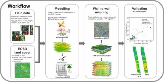
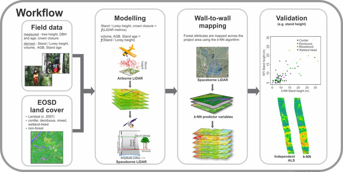
3.1. General Framework

A schematic representation of the methods followed by the MVI project is shown in Figure 2. The 7 stand-level attributes were estimated in each 30 m forest cell within the study area, and the resulting stack of 7 maps is the Satellite Vegetation Inventory (SVI). Information on broad forest type came directly from the landcover map (see Section 3.2). To circumvent the scarcity of field data, as proposed by Mahoney et al. [8], thousands of surrogate FI plots scattered across the project area were created out of selected GLAS footprints with forest attributes estimated using nested models based on ALS data (Section 3.3) and GLAS data (Section 3.4). Specifically, each surrogate plot is the 30 m cell corresponding to the centroid of a GLAS footprint. In that cell, stand height, Lorey’s height, and crown closure attributes were computed as functions of GLAS waveform metrics (Section 3.4). These GLAS models were calibrated using a small set of 43 GLAS footprints that coincided with the 2007 ALS data, where the latter were used to derive an “observed” value of the forest attributes in each of those footprints. The “observed” values were derived from ALS-based models that, in turn, were calibrated with the 38 ground-measured FI plots that had ALS data (Section 3.3). The GLAS surrogate FI plots (Section 3.5) were then used as a reference dataset for the k-NN machine learning algorithm, which used a set of wall-to-wall remote sensing and environmental rasters as feature variables to select the most similar GLAS plots to each target pixel (Section 3.6). The value at the target pixel of the forest attributes was estimated as the mean value in those GLAS plots. An exception was stand age, which was estimated as a power function of k-NN predicted stand height (Section 3.7). Once the SVI was created, it was conflated into a single polygon layer (the MVIv) through a spatial generalization process (Section 3.8). The products were validated using independent data (Section 3.9). Further details on specific methodological steps follow.

3.2. Landcover Mapping

The landcover mapping for phases 1 and 2 followed the general guidelines of the EOSD-LC program [13] with a few exceptions. The Landsat mosaics described in Section 2.4 were partitioned into a few relatively homogeneous zones that were classified separately to account for the diversity of wetland and upland vegetation types within the overall study area. To minimize classification disparities in the seams between phases and zones, water bodies and rivers were used as zone boundaries. All areas outside a given zone were masked out in the input images except for a 10 km buffer around the zone boundary, where the areas of overlap between zones were leveraged by using classified pixels in one zone to help assign labels in subsequent zones. A total of 5 image zones in Phase 1 and seven in Phase 2 were defined. Prior to classification, each zone was stratified into the water, nonvegetation, and low- and high-reflectance vegetation classes (i.e., coniferous and broadleaf, respectively) by manually selecting thresholds in a Normalized Difference Vegetation Index (NDVI) image derived from the Landsat mosaic. Then an unsupervised classification using a K-means clustering algorithm [42], with up to 150 clusters and up to 12 iterations, was run separately for each zone and NDVI stratum. Individual pixels were grouped into spectral clusters using the red, near-infrared, and short-wave infrared bands (bands 3, 4, and 5) and the band 4 texture channel (variance in a 3 by 3 window centred at each pixel). The resulting clusters were then each manually assigned to one of the 22 EOSD classes. Clusters were labelled into the appropriate EOSD class using the reference landcover observations (Section 2.5). Postclassification editing included filling data gaps due to cloud cover, manually delineating rock on exposed mountain tops, and integrating narrow, seasonal rivers and permanent roads that were undetected by the spectral clustering, using the CanVec Series hydrographic and transport features, respectively. The classified products under each image zone were then merged, using seams along water features to form the new landcover map. Ground-truthed locations were used at individual image zones to iteratively improve cluster labelling and to conduct a Phase 2-wide accuracy assessment with confusion matrices to indicate overall agreement as well as producer and user accuracies [43] for three distinct EOSD-LC levels of class detail: level 2 (landcover; treed vs. non-treed), level 4 (vegetation type; 9 classes), and level 5 (density; 17 classes) (Supplementary Materials, Appendix SA2). Owing to the smaller amount of Ducks Unlimited Canada reference data in Phase 1, all ground-truthed observations (Section 2.5) were used for classification; hence the only accuracy assessment performed in Phase 1 was limited to forest type (conifer, broadleaf, and mixedwood) and was based on the agreement with 2 FVI datasets (n = 69,639 forested polygons of >2 ha, Supplementary Materials). For Phase 2, a total of 954 ground-truthed locations were reserved for validation (25% stratified random sample).

3.3. Airborne Laser Scanning Models

ALS metrics were computed for the 38 field plots within the Fort Simpson acquisition (2.3). Various height percentiles and point return ratios were explored in both linear and nonlinear models to predict ground measurements of stand height, Lorey’s height, and crown closure. The best model for each predicted attribute was selected on the basis of 5-fold cross-validation. Models yielding the best goodness of fit statistics (i.e., R² and root mean square error (RMSE), mean prediction error, and largest predictive range) were applied to the ALS dataset for subsequent GLAS modelling [8].

3.4. GLAS Models

As described in Mahoney et al. [8], GLAS global altimetry data (GLA01) and waveform-based range corrections (GLA05) from laser campaigns 2A and 3A were used to calculate waveform metrics for all GLAS footprints within the study area. Several waveform metrics analogous to those used for ALS modelling (e.g., height percentiles, gap fraction) were tested as predictors of stand height, Lorey’s height, and crown closure, where the same criteria used for ALS modelling were employed to determine optimal models for each attribute. Since there were no field data collected at GLAS footprint locations, these models were fitted using data from 43 GLAS footprints that overlapped with the Fort Simpson ALS dataset, where the latter was used to derive an “observed” value of height and crown closure obtained from the ALS models [8].

3.5. Surrogate Plot Dataset

The GLAS models of height and crown closure were applied to GLAS footprints within the study area to create a large set of surrogate FI plots. A subset of 55 GLAS footprints that overlapped boreal transect ALS data was used to decide what filters should be applied to discard unsuitable footprints. Following Mahoney et al. [8], the set of filters that yielded the lowest RMSE and mean absolute error was considered optimal. The selected set included filters that removed footprints with non-treed landcover, with atmosphere saturated or influenced by cloud, on slopes >5%, or with snow. Additional filtering was applied to remove footprints that suffered a disturbance in 2003–2009 (GLAS-Landsat/PALSAR time lag) and to reduce the impact of spatial autocorrelation [37]. Values of total volume and AGB for GLAS footprints that passed the filters were derived from Lorey’s height. Stand volume was likewise derived from their estimated stand height. This involved fitting models of those attributes as a power function of stand (or Lorey’s) height using data from the 194 field plots.

3.6. k-NN Attribute Mapping

The k-NN algorithm [8,44,45] was used to map 5 of the 7 stand-level forest attributes in the SVI (i.e., excluding forest type and stand age). The k-NN algorithm requires a large set of reference pixels with known values of the response variables, here the GLAS-modelled surrogate FI plots. To reduce spatial autocorrelation in the reference dataset, a number of surrogate plots were discarded so that no two plots were closer to each other than an empirically-determined autocorrelation range (500 m in Phase 1 and 350 m in Phase 2) [28]. In addition to the reference dataset, the k-NN algorithm requires a stack of auxiliary raster datasets (also known as feature variables) correlated to the response variables to decide which reference pixels are used to predict response variables for each target pixel. The feature variables were provided by the wall-to-wall satellite, topographic, and climatic geospatial datasets (see Section 2.4 and Section 2.5). For each target forested pixel for which the values of the forest attributes are unknown, the k-NN algorithm finds the k most similar reference pixels. The similarity was measured as the inverse Euclidian distance between the target pixel and the reference pixels within the multidimensional space of feature variables [28,46]. Then, the k-NN predicted values of the 5 attributes for a given target pixel were the mean value of each attribute from the k nearest reference neighbours in the feature space.

There are five characteristics of the k-NN implementation in the MVI project that differ from those in Mahoney et al. [8], and that follow the k-NN workflow detailed in Beaudoin et al. [37]. First, we targeted a broader suite of 5 forest attributes than Mahoney et al. [8], who only predicted 2 forest attributes (stand height, crown closure). Second, we opted for a multivariate k-NN prediction of the 5 response variables to better preserve the covariance among them. Third, we considered a broader suite of 22 candidate feature variables, including 10 Landsat TM spectral, 6 radar PALSAR backscatter, percent tree cover [38], 3 topographic, and 2 climatic variables [39]. Fourth, the best subset of feature variables was derived from a k-NN-based multivariate iterative selection procedure (VarSelection) implemented within the yaImpute R package [47] and as applied by Beaudoin et al. [37]. Fifth, we determined that a value of k = 4 was the best trade-off between (i) the highest possible goodness of fit criterion [45] of predictions with observations and (ii) the lowest possible magnitude of both residual variance and prediction bias [46]. This k-NN workflow was first tested and successfully implemented over Phase 1, as reported in detail in Beaudoin et al. [37], including the assessment of the synergy of Landsat and PALSAR imagery. Then, it was extended to the Phase 2 area with slightly different postprocessing of satellite imagery and selection of best predictor variables.

3.7. Stand Age and Stand Origin

Unlike the other forest attributes, the stand age raster was not created using k-NN; instead, a model was directly applied to each forest pixel on the basis of its estimated stand height. First, the field plot stand ages were partitioned into conifer, broadleaf, and mixedwood groups over 2 generalized forest productivity zones on the basis of their location within a judicious amalgamation of NWT’s level IV ecoregions [29], resulting in 6 datasets for which models of stand age as a power function of stand height were independently fitted. The results of the regional model performances fitted with MVI plots ranged from 0.48 to 0.75 adjusted R² and 20 to 9 years RMSE, respectively. Then the model functions were applied over the study area using the Phase 1 and Phase 2 landcover maps, generalized forest productivity zones, and the stand height raster to create the stand age raster. The stand age raster combined with the date of field inventory was used to determine the origin of the stand, which became the stand origin attribute in the MVI. This step was necessary because stand age is dynamic, making it unsuitable for attribution in a FI. Age adjustment factors were employed from the point of germination to the breast height age defined by the GNWT [48] during translation from stand age to stand origin. The year of stand origin is a static attribute that can be assigned to a particular origin class in the MVI. The MVI decadal origin classes (1930–1939, 1940–1949, etc.) were adapted from the GNWT FVI [48].

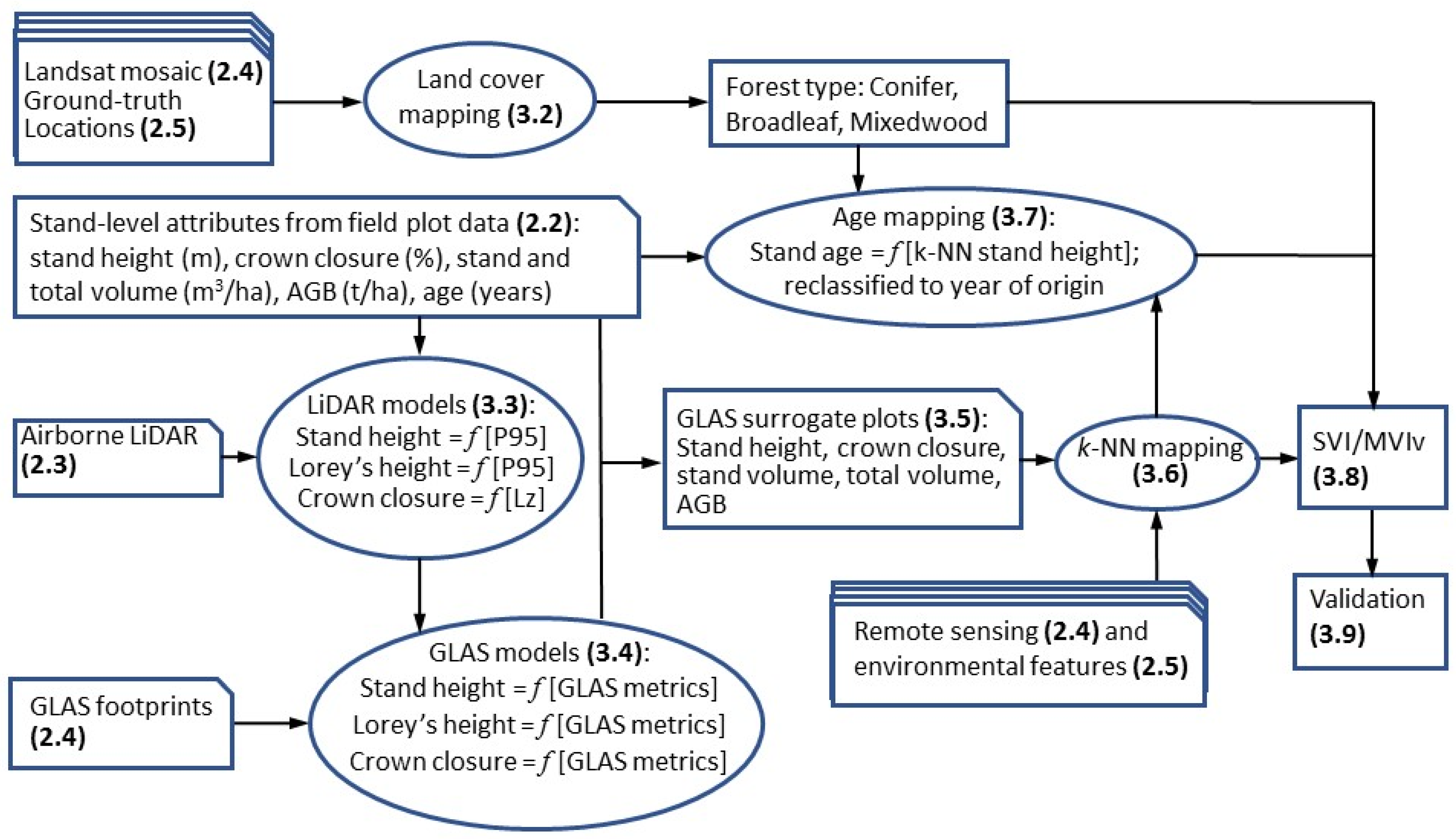
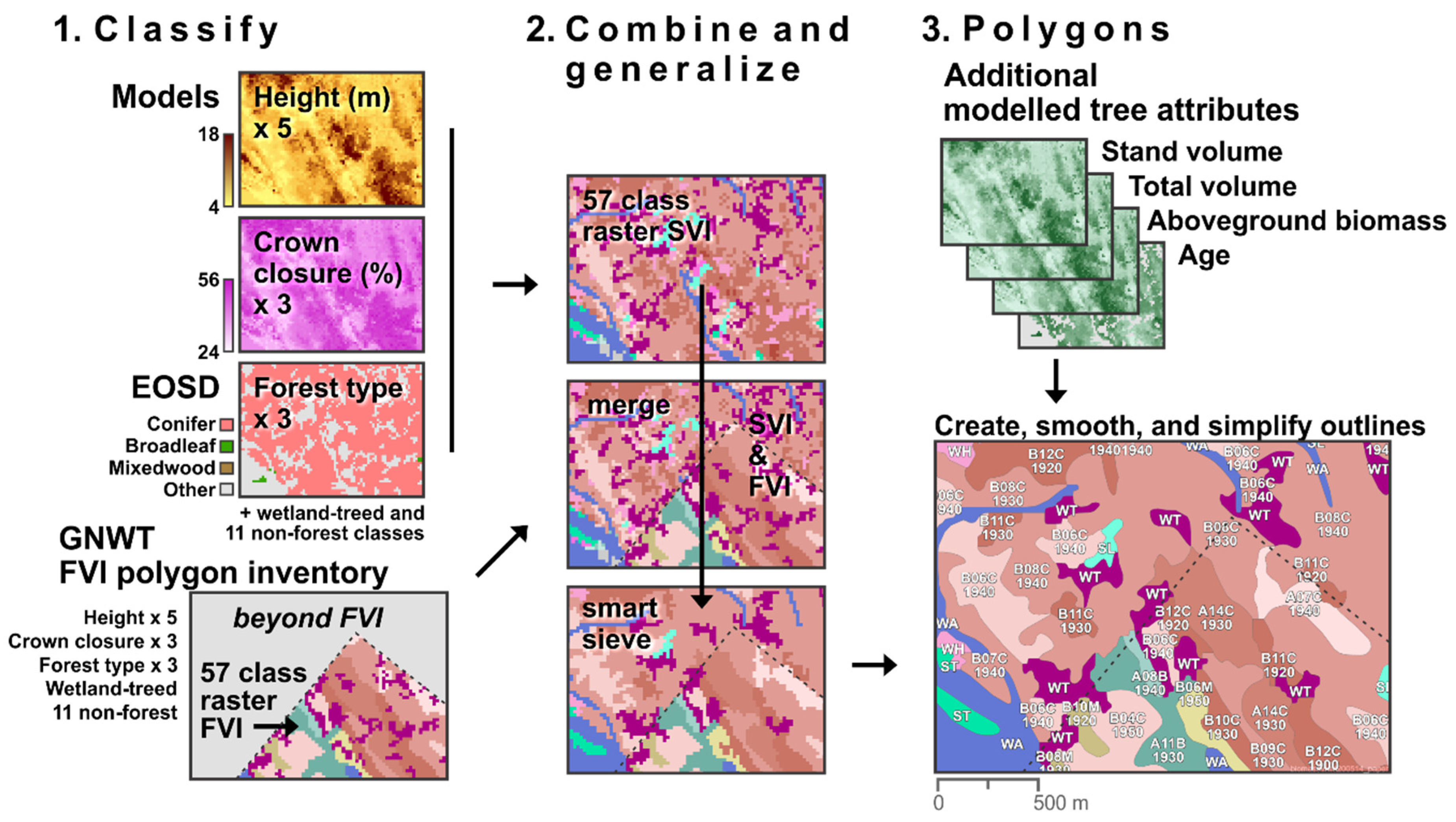
3.8. MVI Polygon Layer

After the stack of 30 m rasters of forest attributes (also known as the Satellite Vegetation Inventory, SVI) was produced, 2 additional goals were to present the SVI as a traditional polygon map and then to combine this information with that from existing aerial photo-interpreted FVIs (16% of the study area, Section 2.1) into a seamless geospatial product, which became the MVIv. To create the MVIv, the following sequence was followed (Figure 3): the SVI was combined into a single categorical raster consisting of 12 nonforest classes and 45 forest classes, where each forest class was a particular combination of forest type, height interval, and crown closure class (

Table 1. Class structure of the polygon version of the Multisource Vegetation Inventory (MVIv).

MVI Attribute	Classes	No. of Classes
Landcover: upland forest 1,2	Conifer, broadleaf, mixedwood	3
Stand height 1	1–6 m, 7–10 m, 11–15 m, 16–20 m, 21 m+	5
Crown closure 1	A: 10%–25%, B: 26%–55%, C: 56%–100%	3
Landcover: wetland treed 2	Wetland treed	1
Landcover: non-treed 2	Shrub tall, shrub low, herb, bryoid, wetland shrub, wetland herb	6
Landcover: nonvegetated 2	Water, exposed rock, barren, roadway, other	5

¹ There are 45 treed forest classes based on combinations of 3 forest types, 5 stand height and 3 crown closure classes. ² Defined in Wulder et al. [13].

). The same classification was applied to the polygons of the existing GNWT FVIs, and the result, which was a thematically generalized version of the original FVI, was rasterized at 30 m pixels. Those pixels replace the pixels in the aforementioned classified raster where the FVI is available. The combined raster was spatially generalized via a “smart sieve” algorithm that iteratively assigned, starting with the smallest, groups of orthogonally connected pixels with the same class to that of the adjacent group belonging to the most similar class according to an expert-defined similarity table. The sieving ended when no groups under 2 ha remained. The resulting raster was converted to polygons with smoothed outlines, labelled using a convention that mimicked that of the GNWT FVIs. The value of the forest attributes in each polygon is the mean of the pixels within the polygon.

3.9. Validation of Forest Attributes

The accuracy assessment of the SVI was based on treed National Forest Inventory ground plots: 52 plots in Phase 1 and 52 in Phase 2. These were used to derive, for each raster, an estimate of the pixel-wise mean error (ME, i.e., bias), the mean absolute error (MAE), their respective confidence intervals, and the RMSE (Supplementary Materials, Section S3.1). To assess the part of the total pixel-wise error that could be attributed to the k-NN alone, we compared the raster values in the centroids of unused, filtered GLAS footprints (nearly 6000 in Phase 1 and almost 4000 in Phase 2) with the value obtained from the GLAS models (Section S3.2). To study the spatial distribution of errors, we applied the ALS models to some acquisitions existing in the area and compared the results in collocated cells (Sections S3.3–S3.5). Finally, to assess results at the forest stand level, we compared the dominant forest type within polygons from three softcopy GNWT FVIs, as well as the mean pixel value of stand height and crown closure within those polygons, with the softcopy calls (Section S3.6). Further information on the materials and methods used in the validation can be found in the validation report in the Supplementary Materials.

4. Results

Here we provide a concise description and interpretation of the main project outcomes.

4.1. Landcover Maps

The image classification process produced a more consistent landcover raster dataset than the circa 2000 EOSD-LC (e.g., no visible seamlines, absence of NoData), which in addition was anchored to a large aerial survey reference dataset of northern boreal vegetation type and density conditions. For Phase 1, the overall agreement with existing FVI data for conifer, broadleaf, and mixedwood forest types was 84% (Table SA2.1). The equivalent confusion matrix for Phase 2 based on ground-truthed locations had an overall agreement of 83% (Table SA2.3), which led us to speculate that the accuracy in Phase 2 should be similar to that in Phase 1, especially since we used similar input and training data, as well as similar methods (but see discussion in Section S4.6). For Phase 2, the agreement with independent validation locations was 71% for the 9-class vegetation type classification (level 4; Table SA2.2) and 86% for the classification between treed and non-treed areas (level 2; Table SA2.4). For both phases, the conifer class was classified with the highest producer (80%–92%) and user (85%–91%) accuracies among the generalized treed classes (Tables SA2.1–SA2.3). Level 4 wetland classes had the lowest producer accuracies and were confused with sparse conifer and shrub classes (Table SA2.2). Level 5 showed a similar pattern, with the wetland treed class classified with one of the lowest producer accuracies and some confusion with the open and sparse conifer classes (Table SA2.5). For brevity, readers are referred to the Supplementary Materials, Appendix SA2, for confusion matrices and accuracy reports.

The most common landcover classes in the study area were conifer open (combined percentage for Phases 1 and 2 of 23%), water (17%), and conifer sparse (12%) (Figure 4a). Secondary landcover classes, each ranging between 8% and 9%, were wetland treed, low shrub, wetland shrub, and conifer dense. Together these seven cover types represented 85% of the study domain. The class bryoids (including reindeer lichen, a key food source for the species-at-risk woodland caribou [49,50]), covered 0.3% of the study area. There were no major differences in the relative abundance of level 4 classes between Phase 1 and Phase 2 except for shrubs (12% higher in Phase 2), wetlands (3% higher in Phase 2), conifers (8% lower in Phase 2), and mixedwood (4.5% lower in Phase 2) (Figure 4b). The higher proportion of shrub in Phase 2 can, in part, be explained by a higher proportion of recently burned areas in Phase 2 than in Phase 1, which in EOSD are typically assigned to the shrub class.

4.2. Models

Thirty-eight field plots were used to calibrate the ALS models of height and crown closure. The best models of stand height and Lorey’s height were linear functions of p95, the height value corresponding to the 95th percentile of points 2 m above the ground (

Table 2. Airborne laser scanning models, parameters, and goodness-of-fit metrics (adjusted (Adj.) R², root mean square error (RMSE)) (n = 38) (stand height and crown closure first reported in Mahoney et al. [8]). P95, height corresponding to the 95th percentile of points 2 m above the ground. Lz, absolute natural logarithm of the proportion of points above 2 m.

Forest Attribute (y)	Units	Model Form	Parameters		Adj. R2	RMSE
			a	b
Stand height	m	HT = a + b P95	0.53	0.96	0.89	1.4
Lorey’s height	m	HL = a + b P95	0.64	0.84	0.89	1.2
Crown closure	%	CC = aLzb	62.78	0.25	0.63	4.8

). The cumulative projected foliage area index (Lz), a logarithmic function of the gap fraction, was the best predictor of crown closure when used in a power function model (see Mahoney et al. [8]).

Forty-three GLAS footprints were available for modelling with the Fort Simpson ALS data. Both stand height and crown closure followed the same model forms as the ALS. The GLAS waveform 85th percentile was the best predictor of height, and a foliage index akin to that used in the ALS models was used to model crown closure with GLAS (

Table 3. Geoscience Laser Altimeter (GLAS) footprint models, parameters, and goodness-of-fit metrics (adjusted (Adj.) R², root mean square error (RMSE)) (n = 43) (HT_GLAS and CC_GLAS first reported in Mahoney et al. [8]). P85, height corresponding to the 85th percentile of waveform energy returned above ground elevation. Lz, absolute natural logarithm of the ratio of the cumulative sum of waveform energy returned from 2 m above ground to the top of the canopy.

Forest Attribute (y)	Units	Model Form	Parameters		Adj. R2	RMSE
			a	b
Stand height	m	HTGLAS = a + b P85	2.30	1.10	0.88	1.3
Lorey’s height	m	HLGLAS = a + b P85	2.46	0.91	0.89	1.1
Crown closure	%	CCGLAS = aLzb	64.63	0.25	0.54	6.5

).

Stand height was used as a predictor of stand volume, and Lorey’s height was used as a predictor of total volume and AGB (

Table 4. Stand volume, total volume, and aboveground biomass (AGB) models, parameters, and goodness-of-fit metrics (adjusted (Adj.) R², root mean square error (RMSE)) based on power function (y = a x ^b) model form (n = 211).

Forest Attribute (y)	Units	Predictor	Parameters		Adj. R2	RMSE
		x	a	b
Stand volume	m3/ha	Stand height	0.61	1.84	0.76	46.8
Total volume	m3/ha	Lorey’s height	1.84	1.69	0.81	59.3
AGB	t/ha	Lorey’s height	2.27	1.45	0.76	35.7

). A 5-fold cross validation of these models generated adjusted R² and RMSE results (

Table 5. Five-fold cross validation of stand volume, total volume, and aboveground biomass (AGB) models.

Forest Attribute (y)	Adj R2 a	RMSE b	Bias c	SD d
Stand volume	0.76	46.7	0.83	46.5
Total volume	0.81	59.2	1.42	59.3
AGB	0.76	35.6	0.28	35.5

^a Adj. R², adjusted R². ^b RMSE, root mean square error. ^c Bias computed as model estimated—observation. ^d SD, standard deviation.

) that were highly similar to model fit results (Table 4), suggesting that these models were robust to the extent that the field data were representative of the forested areas sampled. Two sets of stand age models that used stand height as the predictor variable were developed for conifer, broadleaf, and mixedwood forests that were considered broadly representative of the more productive ecoregions within the Taiga Plains Ecozone [29] (

Table 6. Stand age models as a function of stand height (x), parameters. and goodness-of-fit (adjusted (Adj.) R², root mean square error (RMSE)) metrics based on power function (y = a x ^b) model form. The low-productivity zone consists of all ecoregions within the study area and Taiga Plains Ecozone other than the Liard Plain Mid-Boreal and Liard Upland Mid-Boreal ecoregions that comprise the high-productivity zone [29].

Forest Type	Parameters		Adj.	RMSE
	a	b	R2	(Years)
Low-productivity zone
Conifer (n = 33)	33.78	0.39	0.48	12
Broadleaf (n = 25)	1.82	1.28	0.70	12
Mixedwood (n = 27)	18.30	0.57	0.57	9
High-productivity zone
Conifer (n = 20)	48.78	0.34	0.61	14
Broadleaf (n = 16)	8.53	0.78	0.57	20
Mixedwood (n = 11)	8.63	0.87	0.75	19

). The number of trees used for modelling age was limited as we used only trees for which tree increment cores were available. Model results based on 5-fold cross validation (

Table 7. Five-fold cross validation of stand age models. Adj. R², adjusted R². RMSE, root mean square error. Bias, mean error (computed as model estimate minus observation). SD, standard deviation.

Forest Type	Adj R2	RMSE (Years)	Bias (Years)	SD
Low-productivity zone
Conifer	0.48	12	0.1	12.8
Broadleaf	0.72	12	1.0	11.1
Mixedwood	0.57	8	0.1	7.1
High-productivity zone
Conifer	0.50	15	−2.0	15.4
Broadleaf	0.57	19	0.5	11.3
Mixedwood	0.70	19	2.7	11.5

) were comparable to the generated models (Table 6) with improvements that could be attained from future additional tree increment core collection.

4.3. Surrogate Forest Inventory Plot Dataset

The filters removed roughly 70% of footprints, leaving 7626 GLAS footprints in Phase 1 and 3778 in Phase 2 available as surrogate FI plots (Section 3.5). Out of those, 3600 in Phase 1 and 2157 in Phase 2, which were free from disturbance and farther away from each other than the autocorrelation range, were selected as the reference dataset for k-NN mapping. Over Phase 1, those footprints selected as surrogate FI plots displayed a wider range of values, were taller, and had higher crown closure and larger volume and biomass than in Phase 2 (

Table 8. Descriptive statistics for the surrogate plots used for k-NN estimation by phase.

Forest Attribute	P1 a		P99 b		Mean		Median		SD c
	Phase 1	Phase 2	Phase 1	Phase 2	Phase 1	Phase 2	Phase 1	Phase 2	Phase 1	Phase 2
Stand height (m)	4.1	4.1	31.1	20.4	10.1	7.0	8.1	6.1	5.9	3.0
Crown closure (%)	22.3	21.9	66.2	64.6	41.1	36.3	40.3	34.9	10.3	9.0
Total volume (m3/ha)	20.0	18.8	455.2	231.2	87.4	45.2	53.9	33.8	87.5	37.2
Stand volume (m3/ha)	8.1	8.2	340.6	157.2	54.2	24.8	28.6	17.0	65.4	26.0
Aboveground biomass (t/ha)	2.5	16.7	256.8	128.4	54.8	33.0	36.8	27.6	50.4	20.7

^a P1, first percentile. ^b P99, 99th percentile. ^c SD, standard deviation.

). The median and mean values were also larger in Phase 1 than in Phase 2, and in both Phases, the median was consistently smaller than the mean, indicating a skewed distribution toward smaller values.

4.4. Satellite Vegetation Inventory (SVI, Also Known as Forest Attribute Rasters)

Values of the SVI varied by ecoregion as reflected in the estimated forest attributes, which displayed a wider range and were also taller, of larger crown closure, and of higher volume and biomass for forests in the Mid-Boreal, followed by the high boreal and low subarctic (

Table 9. Descriptive statistics for each of the forest attributes in each Level II ecoregion within the study area.

Forest Attribute	P1 a			P99 b			Mean			Median			SD c
	Mid Boreal	High Boreal	Low Subarctic	Mid Boreal	High Boreal	Low Subarctic	Mid Boreal	High Boreal	Low Subarctic	Mid Boreal	High Boreal	Low Subarctic	Mid Boreal	High Boreal	Low Subarctic
Stand height (m)	4	4	4	22	20	11	9.8	8.5	6.5	9	7	6	4.5	3.4	1.6
Crown closure (%)	22	25	24	59	57	50	40.5	39.1	34.9	41	38	34	8.6	7.2	5.7
Total volume (m3/ha)	20	23	21	291	248	111	82.3	63.1	39.3	34	60	47	5.7	61	44.3
Stand volume (m3/ha)	8	9	9	207	173	71	50.1	36.3	20.7	33	25	17	44.3	31.7	12.1
Aboveground biomass (t/ha)	9	11	17	173	152	74	55.3	44.3	30.7	44	36	28	36.9	27.3	11.4
Stand age (years)	17	25	14	134	107	88	77	74.1	66	75	73	68	19.6	12.5	13.2

^a P1, first percentile. ^b P99, 99th percentile. ^c SD, standard deviation.

).

SVI predictions were reasonable for common conifer stands and somehow poorer in heterogeneous or hilly terrain, complex multistory stands, and less common forest types such as broadleaf. The combined use of both optical and SAR features in the k-NN estimation of forest attributes provided significant improvements compared with estimates derived using only one of these two types of features of up to a 30% reduction in the case of RMSE [37]. In addition to Landsat and PALSAR features, the VarSelection procedure selected a few environmental features (elevation, slope, and a climate index) [37]. In the case of Phase 2, the slope was removed from the feature set because it had an inordinate influence in the selection of the nearest neighbours and actually led to more error in comparison to ground truth independent from the k-NN optimization.

4.5. MVI Polygon Layer

The resulting MVI polygon layer had 1,141,448 polygons in Phase 1 (mean size 17.6 ha, median size 4.5 ha) and 1,618,984 polygons in Phase 2 (mean size 14.9 ha, median size 4.1 ha). The most frequent landcover class by number of polygons was wetland treed and by area was water in both Phases. As a result of the MVI classification structure and dominance of relatively short height and open crown closure forests populated by black spruce and larch, there were 52 forest polygons in Phase 1 and 60 in Phase 2 that exceeded 10,000 ha in size. The largest forest polygon had 47 thousand hectares in Phase 1 and 53 thousand hectares in Phase 2. Both had B08C as the label (crown closure 26%–55%, mean stand height 8 m, conifer).

Of the 23 million hectares classified as a forest (53% of the project area), the most common polygons in both Phases 1 and 2 were conifer-dominated stands whose crown closure ranged from 26% to 55% (crown closure class B, Table 1) and that were 7–10 m in height. This forest type occupied 35% of the forests in Phase 1 and 46% in Phase 2. More productive stands with crown closure >55% (class C) and average stand height greater than 20 m were rare (<2% in Phase 1, and nil in Phase 2), and the majority occurred in the Liard river basin (50,000 ha of this type of stands) and the South Mackenzie plain (30,000 ha), both in the western portion of the Mid-Boreal Ecoregion (Figure 1). In general, the MVI classification resulted in polygon outlines that would resemble those found in a photo-interpreted map if the same classification legend (Table 1) were used (Figure 5).

4.6. Validation

From all of the validation analyses presented in the Supplementary Materials, it appears that the produced rasters provide reasonable estimates of all six attributes given the uncertainties associated with the remote sensing data and the paucity of ground data in the region. The probability-based design of the NFI survey allows us to affirm with great (95%) confidence that, for example, stand height was underestimated by, at the most, an average of 4 m for the 30 m forest cells and that the mean pixel-wise absolute error was at most 4 m or up to 26% of the mean stand height in Phase 1, and 24% in Phase 2 (Section S4.1). Comparison with other independent datasets (unused GLAS footprints (Section S4.2), other ALS data (Sections S4.3–S4.5), and the GNWT FVI (Section S4.6) suggest that these errors may be closer to the lower confidence interval limit than to the upper limit. Overall, the SVI estimates were reasonable for both stand height and crown closure in open conifer stands, which occupy almost 60% of the forested area within the study area. Estimates of all forest attributes were within many reported estimates predicted using ALS data [41]. The poorest estimates were for dense deciduous stands; however, they cover <5% of the forested area within the study area. There was high variability in volume and biomass estimates, with decreasing accuracy in both low (overestimation) and high (underestimation) biomass stands. Although the bias and mean absolute error were lower in Phase 2 than in Phase 1, the relative errors were larger, and the agreement with the reference datasets was more spatially inconsistent. Stand age, which was estimated as a function of stand height, performed surprisingly well in Phase 1 (%RMSE of 35%, or 31 years), but not in Phase 2, where the underestimation bias could be as much as 90 years, owing to the lack of tree ring data in Phase 2 where trees can be very old and still have a low height. In general, error in Phase 2 is likely attributable to the lower mean stand height found in Phase 2, which poses challenges for GLAS height estimation. When estimates are compared with observed values in field plots and lidar plots (Stand height and AGB shown in Figure 6; other attributes show similar patterns), trend lines closely follow the 1:1 line for NFI plots and LiDAR plots from the Boreal Transect (Section 2.5), with a slight overestimation for low values and underestimation for high values. However, for the MVI plots, which were selected for modelling purposes and where the more productive stands are overrepresented, the trend line is on the underestimation side across all the ranges, which is unsurprising given their values are above the regional average. Further observations on the validation results are available in the Supplementary Materials.

5. Discussion

The results of the MVI project were produced by collaborative research efforts that tackled the challenge of how to generate a spatially explicit inventory in a northern boreal environment where site access is difficult and available information is extremely limited. Here we discuss the main contributions of the project, compare its products with others available for the area, briefly describe some uses and applications, mention some limitations and lessons learned, and lay out the plans for a remapping exercise for the reference year 2022.

5.1. Contributions

A key feature of the MVI project was the scaling and modelling of judiciously located field plots across an ecologically broad geographic range with airborne and satellite remote sensing data and other geospatial datasets. This resulted in several contributions:

(1)

A more consistent and accurate satellite landcover map was developed for this project by partitioning the project area into mapping zones separated along the major hydrological features, where the Landsat data for the different zones were calibrated using the same MODIS data. Undertaking classification within a zone helped to produce a more seamless and spatially continuous product [51] than one based on individual Landsat scenes that are then subsequently merged. Successful technology transfer through a training workshop and ongoing support from the CFS has enabled GNWT to undertake landcover mapping in Phase 2 using methods developed in this study.

(2)

Field sampling plots established in the MVI project following National Forest Inventory standards were adopted by GNWT into their permanent sample plot network.

(3)

A scaling approach was devised, tested, and published [8], which incorporated multisource data from field plots, airborne and satellite LiDAR. The k-nearest neighbour mapping method in [8] was refined in [37] to enable the addition of a broader set of forest attributes using a multivariate k-NN process. How to validate the products at various stages was also a subject of considerable effort and value (validation report in Supplementary Materials).

(4)

The incorporation of free archived satellite L-band PALSAR data with Landsat, digital elevation, and climate datasets resulted in substantially improved estimates of forest structure through the synergy of optical and radar data [37]. In particular, RMSE% values were about 15% lower for both stand height and AGB when PALSAR data were employed [37].

(5)

A spatial generalization method was developed that converted the set of 30 m pixel estimates of forest attributes into a single GIS layer consisting of polygons with a complex label akin to that of traditional FIs. The layer seamlessly integrates the FVI where available, providing an invaluable synoptic view of the NWT forest resource.

(6)

Although a detailed cost analysis was not undertaken, a ballpark estimate based on field and airborne data collection costs and personnel time invested in the MVI project suggest that the overall cost of this inventory amounted to a few cents per hectare. Efforts will be undertaken to derive a more precise cost estimate for the circa 2022 remapping effort, but in any case, it is worth noting that a conventional softcopy inventory covering the same area would cost tens of millions of dollars.

5.2. Comparison with Other Similar Products Now Available in the Area

The generation of inventory maps of forest attributes provides a useful characterization of the landscape that supports a wide range of resource management decisions [52]. It is not economically feasible to collect field measurements and produce conventional FIs across all forests in the northern boreal, and particularly so in the NWT [12]. To provide context, 14 separate GNWT FVIs were available, occupying just 38% of Phase 1 and 4% of Phase 2. This problem is not unique, resulting in considerable interest in spaceborne LiDAR (ICESat satellites) as a data source, particularly when combined with datasets that have complete spatial coverage [20,53,54,55]. The integration of airborne/spaceborne LiDAR with other multisource data for large area mapping, including the NWT, has seen increasing traction in the recent literature [22,24,53,56,57]. Although all of these studies generated raster-based estimates of various attributes such as aboveground carbon, AGB, mean canopy height, and canopy cover, none employed locally collected field data specific to this region for calibrating their models, and neither did they generate polygonal maps of specific interest to NWT applications. Beaudoin et al. [37] discuss a comparison with an AGB map from one of these studies [56]. A detailed assessment of the accuracy of the MVI attributes was also undertaken and is reported in the Supplementary Materials.

5.3. Applications

The MVI project was conceived in response to GNWT’s needs for baseline forest information to (i) monitor long-term effects of climate change; (ii) supply a primary vegetation dataset that can be used for cumulative impact monitoring; and (iii) undertake regional forest management planning around communities. The MVI has also been used as a base for building resource selection functions and range plans for boreal (woodland) caribou (Rangifer tarandus caribou) in the NWT [50]. Of particular value was the updated landcover information over the Taiga Plains from which bryoids, wetlands, and sparse/open conifer forests were among the top selected areas in caribou habitat selection modelling on an annual and seasonal basis [50]. GNWT anticipates that regular updates to the inventory will help monitor and assess potential climate-driven changes to forest and vegetation composition that may result from changing fire regime, altered regeneration patterns, melting permafrost, and changes in wetland composition and distribution.

Another application of the MVI is as input to the Carbon Budget Model of the Canadian Forest Sector (CBM-CFS3) within the National Forest Carbon Monitoring, Accounting and Reporting System [14]. The MVI stand age raster can be used to determine the start year of a simulation run within the C budget model tool that uses raster-based, spatially explicit information [58]. The subsequent evolution of each pixel is driven by species-specific yield curves, where the choice of the yield curve in each pixel can be informed by the MVI landcover product. Spatially explicit information about forests contributes to improved calculations of greenhouse gas emissions and removals [58], particularly for northern boreal regions where detailed, current inventory information is often lacking.

5.4. Study Limitations and Lessons Learned

The field, airborne/satellite LiDAR, remote sensing, and other datasets collected over a relatively similar time frame indicative of conditions from 2005 to 2010 no longer reflect the current conditions in burned areas. During the 2010s, there were over 2000 fires that burned nearly seven million ha (Source: https://cfs.nrcan.gc.ca/statsprofile/disturbance/nt accessed 20 July 2020). This has greatly altered the forested landscape of the NWT. Mahoney et al. [8], and the detailed analysis presented in the Supplementary Materials, identified uncertainties in the GLAS models related to topography, background noise, and sensor saturation [59], which increase considerably when canopy height is less than 7 m [60]. In addition, data collection errors, the currency of multisource data, the representativeness of selected field plots over less productive landscapes, and scaling from field and airborne to satellite LiDAR are other factors that contribute to uncertainties in the estimates. Additional field data collection of tree increment cores would also improve age modelling and subsequent determination of stand origin. The paucity of field inventory plots and coincident airborne LiDAR over Phase 2 further exacerbates the uncertainties in estimates of forest attributes, resulting in inferences that are less reliable for the low subarctic ecoregion of the Taiga Plains. Similarly, there was a lack of field data in treed peatlands from which to anchor AGB estimates. An overriding lesson learned for future updates is to ensure in situ data sets are representative of the range of ecological conditions present in the landscape to be mapped. Evaluation of the inventory attributes (SVI) suggested that for any given attribute, small values are generally overestimated, and large values underestimated (Supplementary Materials), consistent with previous studies that employed the k-NN algorithm [28]. The wide confidence intervals obtained from the National Forest Inventory analysis (e.g., the pixel-wise AGB mean absolute error could be as low as 32% or as large as 64% of the mean AGB in Phase 1, Table S1a) stress the need for a denser network of field plots amenable to design-based inference in the region.

5.5. Future Work

We plan to remap the same forest attributes for circa 2022 conditions, using as anchors MVI plots, which were remeasured between 2015 and 2019, and a number of new plots to enhance the representation of less productive areas such as the extensive black spruce peatlands. All of these plots have new ALS data acquired from the Optech Titan Multispectral LiDAR system [61] that will be used to derive new models.

Early investigations into the capabilities of the Optech Titan sensor report highly accurate results of predicting several forest stand characteristics, including AGB [62] and other inventory attributes [63]. Building on these empirical forest attribute models, new models are emerging that exploit the vertical profile of combined spectral and structural information to construct voxel-based representations of biomass structure [64]. These new ALS models will be applied to create a large number of surrogate FI plots (also known as LiDAR plots [41]), this time based on airborne instead of spaceborne LiDAR, which will be scattered along the thousands of kilometres of new ALS transects in the Taiga Plains. The LiDAR plots will be used to train either machine learning (random forests) or artificial intelligence (convolutional neural networks) algorithms that will estimate forest attributes across all the landscapes based on spaceborne LiDAR (ICESat-2), optical, radar, topographic, and climatic features. In particular, circa 2022, cloud-free image composites from several sources (Landsat, PALSAR-2, Sentinel-1/2) will be produced. Other studies employing spatially explicit data that combine FI field plots and remote sensing datasets have reported favourable results from the random forests algorithm [65] and from convolutional neural networks [66]. Such studies support the investigation of alternative mapping approaches. In forests as broadly distributed as in the NWT, the availability and collection of field-based inventory plots to anchor remote sensing models come at a premium. ICESat-2 can potentially extend samples of the airborne ALS transects over the study area if used as a predictor dataset. Early assessment of absolute canopy height of ICESat-2 report results was highly correlated to airborne LiDAR (R² = 0.98) [67], suggesting it is a sensor that offers high sensitivity to vertical forest structure and that it is a potentially useful source of canopy height information in boreal forests [68]. Other input datasets that could improve results include the ArcticDEM, a high-resolution (2 m) spaceborne stereogrammetric digital surface model covering the entire land area north of 60^o latitude [69].

Research opportunities that the MVI project may address in the future include improving knowledge on the spatial distribution of dominant tree species and forest species composition, which would be beneficial to a range of FI applications [12,70]. For example, multispectral airborne LiDAR has the potential for predicting boreal tree species composition [71,72,73]. GNWT is also increasingly using remotely piloted aircraft systems (RPAS, also known as drones) to acquire data for research and other applications [74,75,76]; such data could extend the network of field plots currently limited by physical access and resource availability. The strategic acquisition of RPAS data (specifically point clouds, both LiDAR and photogrammetric), as well as cross-disciplinary leverage of existing RPAS archives and other data, would extend the availability of forest structure information across an ecologically broader range of forest types than what the existing network of FI plots currently offers. This would be of particular value over areas where existing field data are extremely limited, and it provides opportunities to sample other vegetation types such as forested peatlands and wetlands and track recovery dynamics of burned areas. Combined with limited destructive sampling, this could enable the development of biomass models that rely on allometric predictors that can be measured from above, such as height and crown area [77]. One limitation mentioned in Section 5.4 was the estimation of AGB and age of small black spruce in peatlands. This is being addressed by the collection of new field data in support of growth curves that could be used as input to a peatland growth carbon model for national greenhouse gas reporting [78]. These data will also support the development of new AGB models that use ALS data as predictors that should improve future forest attribute maps that better reflect forest conditions in more northerly and less productive environments.

6. Conclusions

Conducting a forest inventory (FI) across forests that are widely and sparsely distributed as in the NWT is a challenging proposition, particularly when physical access and availability of field data are limited. The MVI project was devised as a data augmentation approach where a reconnaissance-level FI (a landcover map) would be accrued with other forest attributes and converted into a strategic-level FI. An existing, circa 2000, EOSD satellite landcover was replaced by a circa 2007 landcover map for Phase 1 and a circa 2010 landcover map for Phase 2 by classifying several homogenous zones partitioned along major drainages. This procedure improved consistency and sensitivity to different landcover types and helped to minimize differences along image seamlines by classifying normalized Landsat TM image mosaics that were subsequently combined into a contiguous landcover map. This updated landcover map served as the basis from which more detailed mapping of forest structure, volume, and AGB was undertaken in forest areas. This was achieved through scaling up a large set of surrogate FI plots that were created from a chain of nested models that linked spaceborne to airborne LiDAR to judiciously selected field plots. Proceeding from the conceptual approach and methods presented in Mahoney et al. [8], this paper describes how a broader suite of forest attributes (stand height, crown closure, total volume, stand volume, AGB, and stand age) was estimated by expanding the set of input feature variables, including radar PALSAR backscatter, and by modifying the k-NN process, described in [37]. Finally, a spatial and semantic generalization process combined the forest attribute rasters in the SVI with the NWT FVI to generate a vector-based polygon layer that broadly resembles a conventional FI map. These two inventory products in raster and polygon formats provide information that is already being used in a range of NWT resource management applications. A comprehensive evaluation of the MVI products using independent National Forest Inventory [79], airborne LiDAR [41], and ICESat GLAS data was undertaken (Supplementary Materials), and data limitations were identified as items to address in future work. The MVI project demonstrated a practical approach for large area forest inventory in remote boreal regions by integrating, modelling, and scaling data from multiple sources, from field plots to the satellite.

References

1. Gillis, M.D.; Leckie, D.G. Forest Inventory Mapping Procedures across Canada; Forestry Canada Information Rep. PI-X-114; Petawawa National Forestry Institute: Chalk River, ON, Canada, 1993.
2. Leckie, D.G.; Gillis, M.D. Forest inventory in Canada with emphasis on map production. For. Chron. 1995, 71, 74–88. [Google Scholar] [CrossRef]
3. Hall, R.J. The roles of aerial photographs in forestry remote sensing image analysis. In Remote Sensing of Forest Environments; Wulder, M.A., Franklin, S.E., Eds.; Springer: New York, NY, USA, 2003; pp. 47–75. [Google Scholar]
4. Castilla, G.; Hird, J.; Maynes, B.; Crane, D.; Cosco, J.; Schieck, J.; McDermid, G. Broadening modern resource inventories: A new protocol for mapping natural and anthropogenic features. For. Chron. 2013, 89, 681–689. [Google Scholar] [CrossRef] [Green Version]
5. Thompson, I.D.; Maher, S.C.; Rouillard, D.P.; Fryxell, J.M.; Baker, J.A. Accuracy of forest inventory mapping: Some implications for boreal forest management. For. Ecol. Manag. 2007, 252, 208–221. [Google Scholar] [CrossRef]
6. Fent, L.; Hall, R.J.; Nesby, R.K. Aerial films for forest inventory: Optimizing film parameters. Photogramm. Eng. Remote Sens. 1995, 61, 281–289. [Google Scholar]
7. Magnussen, S.; Russo, G. Uncertainty in photo-interpreted forest inventory variables and effects on estimates of error in Canada’s National Forest Inventory. For. Chron. 2012, 88, 439–447. [Google Scholar] [CrossRef] [Green Version]
8. Mahoney, C.; Hall, R.J.; Hopkinson, C.; Filiatrault, M.; Beaudoin, A.; Chen, Q.; Mahoney, C.; Hall, R.J.; Hopkinson, C.; Fil-iatrault, M. A Forest Attribute Mapping Framework: A Pilot Study in a Northern Boreal Forest, Northwest Territories, Canada. Remote Sens. 2018, 10, 1338. [Google Scholar] [CrossRef] [Green Version]
9. Gerylo, G.R.; Hall, R.J.; Franklin, E.S.; Smith, L. Empirical relations between Landsat TM spectral response and forest stands near Fort Simpson, Northwest Territories, Canada. Can. J. Remote Sens. 2002, 28, 68–79. [Google Scholar] [CrossRef]
10. Franklin, S.E.; Hall, R.J.; Smith, L.; Gerylo, G.R. Discrimination of conifer height, age and crown closure classes using Landsat-5 TM imagery in the Canadian Northwest Territories. Int. J. Remote Sens. 2003, 24, 1823–1834. [Google Scholar] [CrossRef]
11. Skakun, R.S.; Hall, R.J.; Arsenault, E.; Smith, L.; Cassidy, A.; Lakusta, T.; Beaudoin, A.; Guindon, L. Using multi-sensor satellite imagery to map forest stand attributes in the Mackenzie Valley, NWT. In Proceedings of the International Polar Year GeoNorth Conference, Yellowknife, NWT, Canada, 19–24 August 2007; Available online: https://cfs.nrcan.gc.ca/pubwarehouse/pdfs/27432.pdf (accessed on 1 October 2020).
12. Van der Sluijs, J.; Hall, R.J.; Peddle, D.R. Influence of Field-Based Species Composition and Understory Descriptions on Spectral Mixture Analysis of Tree Species in the Northwest Territories, Canada. Can. J. Remote Sens. 2016, 42, 591–609. [Google Scholar] [CrossRef]
13. Wulder, M.; White, J.; Cranny, M.; Hall, R.J.; Luther, J.; Beaudoin, A.; Goodenough, D.G.; Dechka, A.J. Monitoring Canada’s forests. Part 1: Completion of the EOSD land cover project. Can. J. Remote Sens. 2008, 34, 549–562. [Google Scholar] [CrossRef]
14. Kurz, W.A.; Apps, M.J. Developing Canada’s National Forest Carbon Monitoring, Accounting and Reporting System to Meet the Reporting Requirements of the Kyoto Protocol. Mitig. Adapt. Strat. Glob. Chang. 2006, 11, 33–43. [Google Scholar] [CrossRef]
15. Kurz, W.; Shaw, C.; Boisvenue, C.; Stinson, G.; Metsaranta, J.; Leckie, D.; Dyk, A.; Smyth, C.; Neilson, E. Carbon in Canada’s boreal forest—A synthesis. Environ. Rev. 2013, 21, 260–292. [Google Scholar] [CrossRef]
16. Tomppo, E.; Katila, M. Satellite image-based national forest inventory of Finland. In Proceedings of the IGARSS 1991 Remote Sensing: Global Monitoring for Earth Management, Espoo, Finland, 3–6 June 1991; pp. 1141–1144. [Google Scholar]
17. Nilsson, M. Estimation of Forest Variables Using Satellite Image Data and Airborne Lidar. Ph.D. Thesis, Swedish University of Agricultural Sciences, Umeå, Sweden, 1997. [Google Scholar]
18. Hudak, A.T.; Lefsky, M.A.; Cohen, W.B.; Berterretche, M. Integration of lidar and Landsat ETM+ data for estimating and mapping forest canopy height. Remote Sens. Environ. 2002, 82, 397–416. [Google Scholar] [CrossRef] [Green Version]
19. Saatchi, S.S.; Harris, N.L.; Brown, S.; Lefsky, M.; Mitchard, E.T.A.; Salas, W.; Zutta, B.R.; Buermann, W.; Lewis, S.L.; Hagen, S.; et al. Benchmark map of forest carbon stocks in tropical regions across three continents. Proc. Natl. Acad. Sci. USA 2011, 108, 9899–9904. [Google Scholar] [CrossRef] [PubMed] [Green Version]
20. Lefsky, M.A. A global forest canopy height map from the Moderate Resolution Imaging Spectroradiometer and the Geoscience Laser Altimeter System. Geophys. Res. Lett. 2010, 37, 1–5. [Google Scholar] [CrossRef] [Green Version]
21. Andersen, H.-E.; Strunk, J.; Temesgen, H.; Atwood, D.; Winterberger, K. Using multilevel remote sensing and ground data to estimate forest biomass resources in remote regions: A case study in the boreal forests of interior Alaska. Can. J. Remote Sens. 2011, 37, 596–611. [Google Scholar] [CrossRef]
22. Neigh, C.S.; Nelson, R.F.; Ranson, K.J.; Margolis, H.A.; Montesano, P.M.; Sun, G.; Kharuk, V.; Næsset, E.; Wulder, M.; Andersen, H.-E. Taking stock of circumboreal forest carbon with ground measurements, airborne and spaceborne LiDAR. Remote Sens. Environ. 2013, 137, 274–287. [Google Scholar] [CrossRef] [Green Version]
23. Nelson, R.; Margolis, H.; Montesano, P.; Sun, G.; Cook, B.; Corp, L.; Andersen, H.-E.; Dejong, B.; Pellat, F.P.; Fickel, T.; et al. Lidar-based estimates of aboveground biomass in the continental US and Mexico using ground, airborne, and satellite observations. Remote Sens. Environ. 2017, 188, 127–140. [Google Scholar] [CrossRef] [Green Version]
24. Matasci, G.; Hermosilla, T.; Wulder, M.A.; White, J.C.; Coops, N.C.; Hobart, G.W.; Zald, H.S.J. Large-area mapping of Canadian boreal forest cover, height, biomass and other structural attributes using Landsat composites and lidar plots. Remote Sens. Environ. 2018, 209, 90–106. [Google Scholar] [CrossRef]
25. Luther, J.E.; Fournier, R.A.; Van Lier, O.; Bujold, M. Extending ALS-Based Mapping of Forest Attributes with Medium Resolution Satellite and Environmental Data. Remote Sens. 2019, 11, 1092. [Google Scholar] [CrossRef] [Green Version]
26. Hall, R.J.; Skakun, R.S. Mapping forest inventory attributes across coniferous, deciduous and mixed wood stand types in the Northwest Territories from high spatial resolution QuickBird satellite imagery. In Proceedings of the 28th Canadian Symposium on Remote Sensing/American Society for Photogrammetry and Remote Sensing (ASPRS), Ottawa, ON, Canada, 28 October–1 November 2007; Available online: https://cfs.nrcan.gc.ca/pubwarehouse/pdfs/27753.pdf (accessed on 1 October 2020).
27. Hall, R.J.; Skakun, R.S.; Beaudoin, A.; Wulder, M.A.; Arsenault, E.J.; Bernier, P.Y.; Guindon, L.; Luther, J.E.; Gillis, M.D. Approaches for forest biomass estimation and mapping in Canada. In Proceedings of the IEEE International Geoscience and Remote Sensing Symposium, Honolulu, HI, USA, 25–30 July 2010. [Google Scholar] [CrossRef] [Green Version]
28. Beaudoin, A.; Bernier, P.Y.; Guindon, L.; Villemaire, P.; Guo, X.J.; Stinson, G.; Bergeron, T.; Magnussen, S.; Hall, R.J. Mapping attributes of Canada’s forests at moderate resolution through kNN and MODIS imagery. Can. J. For. Res. 2014, 44, 521–532. [Google Scholar] [CrossRef] [Green Version]
29. Ecosystem Classification Group. Ecological Regions of the Northwest Territories–Taiga Plains; Department of Environment and Natural Resources, Government of the Northwest Territories: Yellowknife, NT, Canada, 2007. Available online: https://www.enr.gov.nt.ca/sites/enr/files/resources/taiga_plains_ecological_land_classification_report.pdf (accessed on 1 October 2020).
30. National Forest Inventory. Canada’s National Forest Inventory Estimation Procedures; Canadian Council of Forest Ministers: Ottawa, ON, Canada, 2004. Available online: https://nfi.nfis.org/resources/estimation/Estimation_procedures_v1.13.pdf (accessed on 1 October 2020).
31. Ung, C.-H.; Bernier, P.; Guo, X.-J. Canadian national biomass equations: New parameter estimates that include British Columbia data. Can. J. For. Res. 2008, 38, 1123–1132. [Google Scholar] [CrossRef]
32. Zhu, Z.; Wulder, M.; Roy, D.P.; Woodcock, C.E.; Hansen, M.C.; Radeloff, V.C.; Healey, S.P.; Schaaf, C.; Hostert, P.; Strobl, P.; et al. Benefits of the free and open Landsat data policy. Remote Sens. Environ. 2019, 224, 382–385. [Google Scholar] [CrossRef]
33. Olthof, I.; Butson, C.; Fernandes, R.; Fraser, R.; Latifovic, R.; Orazietti, J. Landsat ETM+ mosaic of northern Canada. Can. J. Remote Sens. 2005, 31, 412–419. [Google Scholar] [CrossRef]
34. Olthof, I.; Pouliot, D.; Fernandes, R.; Latifovic, R. Landsat-7 ETM+ radiometric normalization comparison for northern mapping applications. Remote Sens. Environ. 2005, 95, 388–398. [Google Scholar] [CrossRef]
35. Luo, Y.; Trishchenko, A.; Khlopenkov, K. Developing clear-sky, cloud and cloud shadow mask for producing clear-sky composites at 250-meter spatial resolution for the seven MODIS land bands over Canada and North America. Remote Sens. Environ. 2008, 112, 4167–4185. [Google Scholar] [CrossRef]
36. Guindon, L.; Bernier, P.; Gauthier, S.; Stinson, G.; Villemaire, P.; Beaudoin, A. Missing forest cover gains in boreal forests explained. Ecosphere 2018, 9, e02094. [Google Scholar] [CrossRef] [Green Version]
37. Beaudoin, A.; Hall, R.J.; Filiatrault, M.; Villemaire, P.; Castilla, G.; Skakun, R.; Guindon, L. Improved k-NN mapping of forest attributes in northern Canada using spaceborne L-band SAR, multispectral and LiDAR data. Remote Sens. 2022, 14, 1181. [Google Scholar] [CrossRef]
38. Hansen, M.C.; Potapov, P.V.; Moore, R.; Hancher, M.; Turubanova, S.A.; Tyukavina, A.; Thau, D.; Stehman, S.V.; Goetz, S.J.; Loveland, T.R.; et al. High-resolution global maps of 21st-century forest cover change. Science 2013, 342, 850–853. [Google Scholar] [CrossRef] [Green Version]
39. Hogg, E.; Barr, A.; Black, T. A simple soil moisture index for representing multi-year drought impacts on aspen productivity in the western Canadian interior. Agric. For. Meteorol. 2013, 178–179, 173–182. [Google Scholar] [CrossRef] [Green Version]
40. Hopkinson, C.; Wulder, M.; Coops, N.; Milne, T.; Fox, A.; Bater, C. Airborne lidar sampling of the Canadian boreal forest: Planning, execution & initial processing. In Proceedings of the 11th International Conference on LiDAR Applications for Assessing Forest Ecosystems, SilviLaser 2011, Hobart, Australia, 16–20 October 2011; Available online: http://scholar.ulethbridge.ca/sites/default/files/hopkinson/files/hopkinson_silvilaser_2011_canada_boreal_lidar.pdf (accessed on 1 October 2020).
41. Wulder, M.A.; White, J.; Bater, C.W.; Coops, N.; Hopkinson, C.; Chen, G. Lidar plots—a new large-area data collection option: Context, concepts, and case study. Can. J. Remote Sens. 2012, 38, 600–618. [Google Scholar] [CrossRef]
42. Tou, J.T.; Gonzalez, R.C. Pattern Recognition Principles; Addison-Wesley Publishing Co.: London, UK, 1974. [Google Scholar]
43. Congalton, R.G.; Green, K. Assessing the Accuracy of Remotely Sensed Data: Principles and Practices, 2nd ed.; Lewis Publishers: Boca Raton, FL, USA, 2009. [Google Scholar]
44. McRoberts, E.R.; Nelson, M.D.; Wendt, D.G. Stratified estimation of forest area using satellite imagery, inventory data, and the k-Nearest Neighbors technique. Remote Sens. Environ. 2002, 82, 457–468. [Google Scholar] [CrossRef]
45. McRoberts, R.E. Estimating forest attribute parameters for small areas using nearest neighbors techniques. For. Ecol. Manag. 2012, 272, 3–12. [Google Scholar] [CrossRef]
46. Beaudoin, A.; Bernier, P.; Villemaire, P.; Guindon, L.; Guo, X.J. Tracking forest attributes across Canada between 2001 and 2011 using a k nearest neighbors mapping approach applied to MODIS imagery. Can. J. For. Res. 2018, 48, 85–93. [Google Scholar] [CrossRef] [Green Version]
47. Crookston, N.L.; Finley, A.O. yaImpute: AnRPackage forkNN Imputation. J. Stat. Softw. 2008, 23, 1–16. [Google Scholar] [CrossRef] [Green Version]
48. Government of Northwest Territories. Northwest Territories Forest Vegetation Inventory Standards with Softcopy Supplements, v4.0; Technical Report; Government of Northwest Territories: Yellowknife, NT, Canada, 2012.
49. McMullin, R.T.; Thompson, I.D.; Lacey, B.W.; Newmaster, S.G. Estimating the biomass of woodland caribou forage lichens. Can. J. For. Res. 2011, 41, 1961–1969. [Google Scholar] [CrossRef]
50. DeMars, C.; Hodson, J.; Kelly, A.; Lamontagne, E.; Smith, L.; Groenewegen, K.; Davidson, T.; Behrens, S.; Cluff, D.; Gurarie, E. Influence of landcover, fire and human disturbance on habitat selection by boreal caribou in the NWT. Report prepared for Project 202 of the Government of the Northwest Territories Department of Environment and Natural Resources, Northwest Territories Cumulative Impact Monitoring Program. 2021; unpublished work. [Google Scholar]
51. Olthof, I.; Latifovic, R.; Pouliot, D. Development of a circa 2000 land cover map of northern Canada at 30 m resolution from Landsat. Can. J. Remote Sens. 2009, 35, 152–165. [Google Scholar] [CrossRef]
52. Corona, P. Integration of forest mapping and inventory to support forest management. iFores–Biogeosci. For. 2010, 3, 59–64. [Google Scholar] [CrossRef] [Green Version]
53. Wulder, M.A.; White, J.C.; Nelson, R.F.; Næsset, E.; Ørka, H.O.; Coops, N.C.; Hilker, T.; Bater, C.W.; Gobakken, T. Lidar Sampling for Large-Area Forest Characterization: A Review. Remote Sens. Environ. 2012, 121, 196–209. [Google Scholar] [CrossRef] [Green Version]
54. Baccini, A.; Walker, W.; Carvalho, L.; Farina, M.; Sulla-Menashe, D.; Houghton, R.A. Tropical forests are a net carbon source based on aboveground measurements of gain and loss. Science 2017, 358, 230–234. [Google Scholar] [CrossRef] [Green Version]
55. Duncanson, L.; Neuenschwander, A.; Hancock, S.; Thomas, N.; Fatoyinbo, T.; Simard, M.; Silva, C.A.; Armston, J.; Luthcke, S.B.; Hofton, M.; et al. Biomass estimation from simulated GEDI, ICESat-2 and NISAR across environmental gradients in Sonoma County, California. Remote Sens. Environ. 2020, 242, 111779. [Google Scholar] [CrossRef]
56. Wang, J.A.; Baccini, A.; Farina, M.; Randerson, J.T.; Friedl, M.A. Disturbance suppresses the aboveground carbon sink in North American boreal forests. Nat. Clim. Chang. 2021, 11, 435–441. [Google Scholar] [CrossRef]
57. Margolis, H.A.; Nelson, R.F.; Montesano, P.M.; Beaudoin, A.; Sun, G.; Andersen, H.-E.; Wulder, M.A. Combining satellite lidar, airborne lidar, and ground plots to estimate the amount and distribution of aboveground biomass in the boreal forest of North America. Can. J. For. Res. 2015, 45, 838–855. [Google Scholar] [CrossRef] [Green Version]
58. Boisvenue, C.; Smiley, B.P.; White, J.C.; Kurz, W.A.; Wulder, M.A. Improving carbon monitoring and reporting in forests using spatially-explicit information. Carbon Balance Manag. 2016, 11, 23. [Google Scholar] [CrossRef] [PubMed] [Green Version]
59. Lee, S.; Ni-Meister, W.; Yang, W.; Chen, Q. Physically based vertical vegetation structure retrieval from ICESat data: Validation using LVIS in White Mountain National Forest, New Hampshire, USA. Remote Sens. Environ. 2011, 115, 2776–2785. [Google Scholar] [CrossRef]
60. Nelson, R. Model effects on GLAS-based regional estimates of forest biomass and carbon. Int. J. Remote Sens. 2010, 31, 1359–1372. [Google Scholar] [CrossRef]
61. Hopkinson, C.; Chasmer, L.; Gynan, C.; Mahoney, C.; Sitar, M. Multisensor and Multispectral LiDAR Characterization and Classification of a Forest Environment. Can. J. Remote Sens. 2016, 42, 501–520. [Google Scholar] [CrossRef]
62. Dalponte, M.; Ene, L.T.; Gobakken, T.; Næsset, E.; Gianelle, D. Predicting Selected Forest Stand Characteristics with Multispectral ALS Data. Remote. Sens. 2018, 10, 586. [Google Scholar] [CrossRef] [Green Version]
63. Goodbody, T.; Tompalski, P.; Coops, N.; Hopkinson, C.; Treitz, P.; Van Ewijk, K. Forest Inventory and Diversity Attribute Modelling Using Structural and Intensity Metrics from Multi-Spectral Airborne Laser Scanning Data. Remote Sens. 2020, 12, 2109. [Google Scholar] [CrossRef]
64. Okhrimenko, M.; Coburn, C.; Hopkinson, C. Multi-Spectral Lidar: Radiometric Calibration, Canopy Spectral Reflectance, and Vegetation Vertical SVI Profiles. Remote Sens. 2019, 11, 1556. [Google Scholar] [CrossRef] [Green Version]
65. Zhang, L.; Suganthan, P.N. Random Forests with ensemble of feature spaces. Pattern Recognit. 2014, 47, 3429–3437. [Google Scholar] [CrossRef]
66. Ayrey, E.; Hayes, D.J. The Use of Three-Dimensional Convolutional Neural Networks to Interpret LiDAR for Forest Inventory. Remote Sens. 2018, 10, 649. [Google Scholar] [CrossRef] [Green Version]
67. Neuenschwander, A.L.; Magruder, L.A. Canopy and Terrain Height Retrievals with ICESat-2: A First Look. Remote Sens. 2019, 11, 1721. [Google Scholar] [CrossRef] [Green Version]
68. Neuenschwander, A.; Guenther, E.; White, J.C.; Duncanson, L.; Montesano, P. Validation of ICESat-2 terrain and canopy heights in boreal forests. Remote Sens. Environ. 2020, 251, 112110. [Google Scholar] [CrossRef]
69. Puliti, S.; Hauglin, M.; Breidenbach, J.; Montesano, P.; Neigh, C.; Rahlf, J.; Solberg, S.; Klingenberg, T.; Astrup, R. Modelling above-ground biomass stock over Norway using national forest inventory data with ArcticDEM and Sentinel-2 data. Remote Sens. Environ. 2019, 236, 111501. [Google Scholar] [CrossRef]
70. Fassnacht, F.E.; Latifi, H.; Stereńczak, K.; Modzelewska, A.; Lefsky, M.; Waser, L.T.; Straub, C.; Ghosh, A. Review of studies on tree species classification from remotely sensed data. Remote Sens. Environ. 2016, 186, 64–87. [Google Scholar] [CrossRef]
71. Axelsson, A.; Lindberg, E.; Olsson, H. Exploring Multispectral ALS Data for Tree Species Classification. Remote Sens. 2018, 10, 183. [Google Scholar] [CrossRef] [Green Version]
72. Budei, B.C.; St-Onge, B.; Hopkinson, C.; Audet, F.-A. Identifying the genus or species of individual trees using a three-wavelength airborne lidar system. Remote Sens. Environ. 2018, 204, 632–647. [Google Scholar] [CrossRef]
73. Kukkonen, M.; Maltamo, M.; Korhonen, L.; Packalen, P. Multispectral Airborne LiDAR Data in the Prediction of Boreal Tree Species Composition. IEEE Trans. Geosci. Remote Sens. 2019, 57, 3462–3471. [Google Scholar] [CrossRef]
74. Fraser, R.H.; Van der Sluijs, J.; Hall, R.J. Calibrating Satellite-Based Indices of Burn Severity from UAV-Derived Metrics of a Burned Boreal Forest in NWT, Canada. Remote Sens. 2017, 9, 279. [Google Scholar] [CrossRef] [Green Version]
75. Van Der Sluijs, J.; Kokelj, S.V.; Fraser, R.H.; Tunnicliffe, J.; Lacelle, D. Permafrost Terrain Dynamics and Infrastructure Impacts Revealed by UAV Photogrammetry and Thermal Imaging. Remote Sens. 2018, 10, 1734. [Google Scholar] [CrossRef] [Green Version]
76. Van Der Sluijs, J.; Mackay, G.; Andrew, L.; Smethurst, N.; Andrews, T.D. Archaeological documentation of wood caribou fences using unmanned aerial vehicle and very high-resolution satellite imagery in the Mackenzie Mountains, Northwest Territories. J. Unmanned Veh. Syst. 2020, 8, 186–206. [Google Scholar] [CrossRef]
77. Wagers, S.; Castilla, G.; Filiatrault, M.; Sanchez-Azofeifa, A. Using TLS-measured Tree Attributes to Estimate Aboveground Biomass in Small Black Spruce Trees. Forests 2021, 12, 1521. [Google Scholar] [CrossRef]
78. Bona, K.A.; Shaw, C.; Thompson, D.K.; Hararuk, O.; Webster, K.; Zhang, G.; Voicu, M.; Kurz, W.A. The Canadian model for peatlands (CaMP): A peatland carbon model for national greenhouse gas reporting. Ecol. Model. 2020, 431, 109164. [Google Scholar] [CrossRef]
79. Gillis, M.D.; Omule, A.Y.; Brierley, T. Monitoring Canada’s forests: The National Forest Inventory. For. Chron. 2005, 81, 214–221. [Google Scholar] [CrossRef]
80. Natural Resources Canada. Canada’s National Forest Inventory Ground Sampling Guidelines, Version 5.0. Natural Resources Canada, Canadian Forest Service. 2008. Available online: https://nfi.nfis.org/en/ground_plot (accessed on 27 November 2020).
81. McRoberts, R.E. Diagnostic tools for nearest neighbors techniques when used with satellite imagery. Remote Sens. Environ. 2009, 113, 489–499. [Google Scholar] [CrossRef]
82. Lambert, M.-C.; Ung, C.-H.; Raulier, F. Canadian national tree aboveground biomass equations. Can. J. For. Res. 2005, 35, 1996–2018. [Google Scholar] [CrossRef]
83. Wulder, M.A.; White, J.C.; Luther, J.E.; Strickland, G.; Remmel, T.K.; Mitchell, S.W. Use of vector polygons for the accuracy assessment of pixel-based landcover maps. Can. J. Remote Sens. 2006, 32, 268–279. [Google Scholar] [CrossRef]
Figure 1. Overview of the Multisource Vegetation Inventory (MVI) project area. The ~151,700 km2 Phase 1 has 2007 as the reference year, covers mostly the Taiga Plains Mid-Boreal (light green) and HighBoreal (dark green) ecoregions, and overlaps with ~36,600 km2 of Government of the Northwest Territories (GNWT) Forest Vegetation Inventories (FVIs, purple polygons). The 244,000 km2 Phase 2 has 2010 as the reference year, covers mostly the Taiga Plains Low Subarctic Ecoregion (brown), and overlaps with ~9500 km2 of GNWT FVIs. Main populated places are shown as white dots.
Remotesensing 14 01108 g001
Figure 2. Flowchart of the materials and methods in this study, with reference to the relevant subsections in brackets. Notched rectangles represent inputs, ellipses represent models or processes, and rectangles represent outputs.
Remotesensing 14 01108 g002
Figure 3. Overview of the spatial generalization of the raster maps into polygons in the vector version of the Multisource Vegetation Inventory produced in this study (MVIv). The dashed grey line in the lower insets represents the virtual seamline between the Forest Vegetation Inventory (FVI) and the Satellite Vegetation Inventory (SVI), which does not exist in the final vector product. For forest polygons, the first letter in the label indicates the crown closure class, the next 2 digits are the mean stand height, the last letter is the broad forest type, and the 4 digits below are the origin year (e.g., B11C means a conifer stand of 11 m height and crown closure class B–26%–55%). EOSD is the Earth Observation for Sustainable Development of Forests; GNWT is the Government of the Northwest Territories.
Remotesensing 14 01108 g003
Figure 4. Histogram of the mapped landcover classes for two levels of classification detail: (a) level 5 (vegetation type plus density; 17 classes), and (b) level 4 (vegetation type; 9 classes), for Phases 1 and 2 of the MVI project, roughly corresponding to southern and central Taiga Plains, respectively.
Remotesensing 14 01108 g004
Figure 5. Sample Multisource Vegetation Inventory (MVIv) map for a 1.0 by 1.16 km area some 50 km south of Fort Simpson. The left inset shows the area with the landcover map as a backdrop. The backdrop of the central inset is a Quickbird image of the same area taken in August 2006. The first letter in a polygon’s label is the density class (Table 1), the next 2 digits are the mean stand height, the last letter is the broad forest type (conifer, broadleaf, or mixedwood), and the 4 digits below are the origin year. The photos to the right show 3 ground plots (yellow dots in the central inset) of different forest types.
Remotesensing 14 01108 g005
Figure 6. Scatterplots of predicted (by the Satellite Vegetation Inventory, SVI) vs. observed values of stand height and aboveground biomass (AGB) for forest inventory (FI) field plots (both from the National Forest Inventory, NFI, and the Multi-source Vegetation Inventory, MVI) and LiDAR plots (from Boreal Transect Airborne Laser Scanning dataset, BT-ALS) within the project area. Trend lines for each dataset are shown as dashed lines and the 1:1 line as a solid line.
Remotesensing 14 01108 g006