Technical Note

The Possible Seismo-Ionospheric Perturbations Recorded by the China-Seismo-Electromagnetic Satellite

by
Zeren Zhima
,
Rui Yan
,
Jian Lin
,
Qiao Wang
,
Yanyan Yang
,
Fangxian Lv
,
Jianping Huang
,
Jing Cui
,
Qinqin Liu
,
Shufan Zhao
,
Zhenxia Zhang
,
Song Xu
,
Dapeng Liu
,
Wei Chu
,
Keying Zhu
,
Xiaoying Sun
,
Hengxin Lu
,
Feng Guo
,
Qiao Tan
,
Na Zhou
,
Dehe Yang
,
He Huang
,
Jie Wang
and
Xuhui Shen
*
add Show full author list remove Hide full author list
National Institute of Natural Hazards, Ministry of Emergency Management of China, Beijing 100085, China
*
Author to whom correspondence should be addressed.
Remote Sens. 2022, 14(4), 905; https://doi.org/10.3390/rs14040905
Submission received: 27 December 2021 / Revised: 7 February 2022 / Accepted: 10 February 2022 / Published: 14 February 2022

Abstract

:
Driven by the objective of earthquake disaster prevention and mitigation, China launched the Zhangheng mission to build a stereoscopic earthquake monitoring system from the lithosphere to space. This report briefly presents the possible seismic ionospheric disturbances recorded by the first probe of the Zhangheng mission, which is known as the China-Seismo-Electromagnetic Satellite (CSES). The routine data preprocessing and seismo-ionospheric information analysis methods are briefly introduced. The possible seismo-ionospheric disturbances that appeared during the strong shallow earthquakes (with a magnitude over 7 and a depth shallower than 30 km) are analyzed by using CSES and other multi-source data. Investigating seismo-ionospheric mechanisms requires multidisciplinary knowledge involving geophysics, atmosphere/ionosphere physics, geochemistry/atmospheric chemistry, etc. We state that the results from the CSES scientific application center are preliminary, calling for international scientists to contribute to the seismo-ionospheric perturbation phenomena, which is one of the most challenging scientific problems.

1. Introduction

Strong earthquakes (EQs) are one of the most destructive natural hazards, claiming countless deaths and economic losses in human history. The diversity and scale of EQ activity are daunting; however, the earthquake monitoring capabilities of human society still lack development. Promoting earthquake disaster prevention and reduction capabilities is a common issue faced by all countries worldwide.
The abnormal geophysical and geochemical variation around the EQ preparation zone is interpreted as the seismic precursors [1,2,3]. Electromagnetic signals are regarded as the most promising candidate for short-term earthquake prediction [4,5,6]. With the development of space technology, by the early 1980s, scientists found abnormal electromagnetic emissions, plasma parameter irregularities, and energetic particle precipitations over seismic fault zones from electromagnetic satellite observations [3,7,8,9]. For example, Larkina et al. [7] reported an abnormal electromagnetic field intensity enhancement over the seismic zones from the Intercosmos 19 satellite data. Pulinets and Ouzounov [10] systemically summarized previous studies and concluded that the seismic signals can propagate upward from the lithosphere to the atmosphere and ionosphere, in particular circumstances, even up to the inner magnetosphere.
These new scientific findings bring hope for a breakthrough in earthquake science. Several countries have started building dedicated electromagnetism satellites to monitor these earthquake precursors from space. In the early 21st century, France launched the DEMETER (Detection of Electromagnetic Emissions Transmitted from Earthquake Regions) satellite mission, which successfully operated from December 2004 to December 2010, for studying ionospheric perturbations caused by earthquakes, volcanic eruptions, and human activities [11]. Since then, increasing attention has been given to the seismo-ionospheric disturbances phenomena. Much evidence on possible seismo-ionospheric precursor signatures has been accumulated after extensive studies have been carried out.
Abnormal electromagnetic emissions in a broad frequency range were observed over the epicenter zones or their conjugated points during the impending earthquake time [11,12,13,14]. Nemec et al. [14] statistically evaluated the abnormal electromagnetic field before M 4.8+ shallow-depth EQs by using 3.5 years of DEMETER data and confirmed the existence of a very small but statistically significant decrease in the electromagnetic wave intensity before the mainshock time. The ionospheric parameter irregularity at different altitudes over the EQ preparation zones is most commonly reported [9,15,16,17]. For example, Zhao et al. [15] reported an unusual large-scale enhancement of electron density during the 2008 great Wenchuan earthquake. Marchetti et al. [18] statistically analyzed the variation in the magnetic field and electron density recorded by Swarm satellites and reported anomalies starting about 40 days before the beginning of the seismic sequence, coinciding and following surface and atmospheric alterations. Energetic particle precipitation was also observed during the seismic time [11].
Driven by the objective of earthquake disaster prevention and mitigation, China has been devoted to building a stereoscopic earthquake monitoring system from ground to space, planning to launch a series of Low-Earth-Orbit (LEO) electromagnetism micro-satellites in the following decades step by step [19]. This mission is called the Zhangheng mission, named after the ancient Chinese scientist Zhangheng who invented the world’s first seismo-scope in the second-century CE.
The first electromagnetism microsatellite of the Zhangheng mission, known as the China Seismo-Electromagnetic Satellite (CSES or ZH-1), was successfully launched into a sun-synchronous circular orbit at an altitude of 507 km in the upper ionosphere [19]. TheCSES flies 15.2 orbits around the Earth per day at the local time around 02:00 a.m. (nightside) and 2:00 p.m. (dayside). It has a 5 days revisiting period for the same area. Until now, the CSES has been steadily operating in orbit for over four years. Its identical successor satellite will be launched to the same orbit space around February 2023. This paper briefly reports how the CSES scientific application center analyzes seismic activities using satellite data.

2. Satellite and Payloads

The CSES is specially designed to monitor the ionospheric perturbations associated with seismic activities in the lithosphere. It carries eight types of scientific payloads, including 13 individual instruments to acquire the global geomagnetic field, electromagnetic field/waves, plasma parameters, and energetic particles data. The onboard configuration was introduced by Shen et al. [19]. It also benefits space physics-related studies (e.g., space weather, ionospheric irregularities, and plasma environment). There are two working modes for payload operation: survey and burst mode. The former is operated along the whole orbit trajectory with lower sampling rates; the latter is only triggered above the global main seismic belts with a higher sampling rate. Here, we briefly introduce the scientific payloads as follows. Details of the scientific payloads are listed in Table 1.
The geomagnetic field is detected by the high-precision magnetometer (HPM), which consists of two tri-axial fluxgate magnetometers (FGMs) [20] and one coupled dark-state magnetometer (CDSM) [21]. The FGMs provide the magnetic field vector data in the frequency range from DC (Direct Current) to 15 Hz, and the CDSM serves as a reference to the FGM by providing the scalar value of the total magnetic field. A tri-axial search coil magnetometer (SCM) detects the alternating magnetic field in the frequency range from ~10 Hz to 20 kHz [22], providing data in the three detection frequency bands: ULF (Ultra-Low-Frequency, 10–200 Hz), ELF (Extremely-Low-Frequency, 200 Hz–2.2 kHz), and VLF (Very-Low-Frequency, 1.8 kHz–20 kHz). An electric field detector (EFD) measures the spatial electric field in the frequency band from DC to 3.5 MHz [23], providing data in the four detection frequency bands: ULF (DC-16 Hz), ELF (6 Hz–2.2 kHz), VLF (1.8 kHz–20 kHz), and HF (High-Frequency, 18 kHz–3.5 MHz). One advantage of the CSES satellite is that it provides high-resolution six-component electromagnetic field waveform data in ULF/ELF bands continuously along the whole orbit trajectory in the survey mode, allowing us to examine the wave propagation parameters at any time of interest. The waveform data of VLF/HF is downlinked only during burst mode due to the limitation of telemetry capability.
For the ionospheric plasma parameter detection, a Langmuir probe (LAP) and a set of plasma analyzer packages (PAPs) [24] provide the in situ ionospheric plasma parameters (electron and ion); a GNSS occultation receiver (GOR), and a tri-band beacon (TBB) transmitter together with about 15 ground-based receivers [25] provide the ionospheric profile parameters, such as the TEC (total electron content), electron density profile, and ionospheric scintillation index. For the energetic particles, there are a set of high-energy-particle packages (HEPPs) [26], and a high-energy-particle detector (HEPD) [27] provided by the Italian Space Agency, jointly detecting the energetic particles in an energy level range from ~0.1 MeV to 200 MeV.
The first six-month in-orbit commission tests demonstrate that the scientific instruments generally perform well, except for the PAP, EFD, and TBB, which have some defects in different aspects. PAP was contaminated after four months in orbit, leading to lower absolute values than expected; further evaluation suggests that the relative values of ion densities can be used in scientific applications. The EFD is heavily interfered with by the satellite-internal communication over the equatorial region and has a high noise level in the HF band. The middle frequency band (400 MHz) of the TBB (needs the ground-based receivers to realize the coherent beacon system) malfunctioned after launch, so the data quality of the TBB is still under evaluation. We suggest that extra caution is required when using the PAP, EFD, and TBB for scientific research.
The scientific data are packed into HDF (Hierarchical Data Format) with the descending (orbit path from north pole to south pole) and ascending (from south to north) half-orbit data files. There are five levels of data in total based on the working principles of each payload, which are described as follows: Level 0: The data are reconstructed after a series of preprocessing, including frame synchronization, de-randomization, decoding, and de-formatting on the raw telemetry data.
Level 1: The data obtained after general error elimination, physical unit conversion, format conversion, etc. based on the Level-0 data.
Level 2: The calibrated physical values correspond to Level 1 data with orbit information after coordination system transformation and necessary data inversion.
Level 2A: Only the EFD in the ULF band and GOR deliver the Level 2A data. For the EFD, Level 2A is generated after eliminating the Vs × B effect in the ULF band, where vs. is the satellite’s velocity and B is the geomagnetic field. For GOR data, it is the TEC values obtained after conversion with precision orbit determination information on Level 2.
Level-3: Time sequential data along satellite orbits generated after resampling, necessary spectral analysis based on Level-2 data.
Level-4: The global interpolation maps of physical values from Level-2 data.
The Level 2 data products that can be directly used for scientific application are accessible via the website to the international scientific community (http://leos.ac.cn accessed on 26 December 2021).

3. Data Preprocessing Methods

The ionosphere is easily disturbed by various natural and artificial sources, such as the geomagnetic storms that mainly originate from the Sun or the inner magnetosphere, the intense lightning activity generated from the atmosphere, or the artificial VLF radio waves emitted by powerful terrestrial transmitters. Therefore, before searching for the seismic information from the satellite data, it is necessary to eliminate any possibilities from all other non-earthquake sources. Several data preprocessings are routinely operated to avoid non-EQ disturbance sources.
Step 01: Data cleaning, through which the orbit data affected by satellite control operations or the other artificial experiments are directly excluded, according to the health condition data of the platform and payloads.
Step 02: Space-weather condition check. Compared to the disturbance induced by the solar wind, geomagnetic storms, or lightning activities, the influence from earthquakes is relatively feeble. Under the disturbed space-weather conditions (Dst ≤ −30 nT or Kp ≥ 3), we usually do not analyze the seismo-ionospheric disturbances. That does not mean it is impossible to extract seismic signals under disturbed space-weather conditions. As the physical processes of the seismo-ionospheric phenomena are still poorly understood, selecting the quiet space weather condition can avoid many complicated factors. Additionally, as most previous studies have carried out, we mainly focus on the nighttime data to avoid the complicated ionospheric ionization effects in the daytime.
Step 03: The EQ influential area selection. According to the empirical equation of the earthquake preparation zone put forward by Dobrovolsky et al. [28], the influential zone of an earthquake is roughly computed by the equation R = 10 0.43 M , where R is the diameter of the influential earthquake zone in the km scale, and M is the magnitude of the EQ. For convenience, considering the projection feature of a satellite orbit on the ground, we choose a square area, that is, the epicenter ± 5° area for a magnitude 6 EQ and epicenter ± 10° for a magnitude 7 EQ.
Step 04: Frequency band selection is essential for preprocessing electromagnetic data. The electromagnetic field or waves can be easily interrupted by parasitic signals or other interference sources, which cause uncertainties or errors. For example, below 200 Hz, the interferences originating from instruments or satellite platforms, such as electrostatic turbulence from solar panels or magnetic torque, must be carefully excluded [12]. Selecting a frequency range free of artificial interferences is essential before searching for seismic-related emissions. According to the calibration tests in orbit, at the frequency of 27.5 Hz and its harmonics (from 2 to 5 times and 8–12 times), the SCM data are influenced by the magnetic torque that generates a magnetic moment to maintain the satellite platform position. Over the equatorial area, the electric field data in ULF/ELF/VLF bands are interfered with by the internal communication signals of the satellite platform.

4. Results

The CSES has been steadily operating in the topside ionosphere for over four years. As the CSES launched on 2 February 2018, there have been 38 strong shallow EQs (M 7+, depth shallower than 100 km) worldwide (http://www.ceic.ac.cn/ accessed on 26 December 2021) until 1 December 2021; the epicenter distribution is shown in Figure 1. Previous studies [6,11,14,29] have demonstrated that the seismo-ionospheric perturbation phenomena predominately appear during the shallow strong EQs, so we mainly focus on the strong EQs with a depth shallower than 30 km in this report. The possible seismic ionospheric disturbances are listed in Table 2, and the specific analysis methods are introduced in the following. All the listed information represents possible seismic anomalies; they still need more evidence before confirming them. We share these preliminary results with the public, calling for global efforts for further study with profound methods.

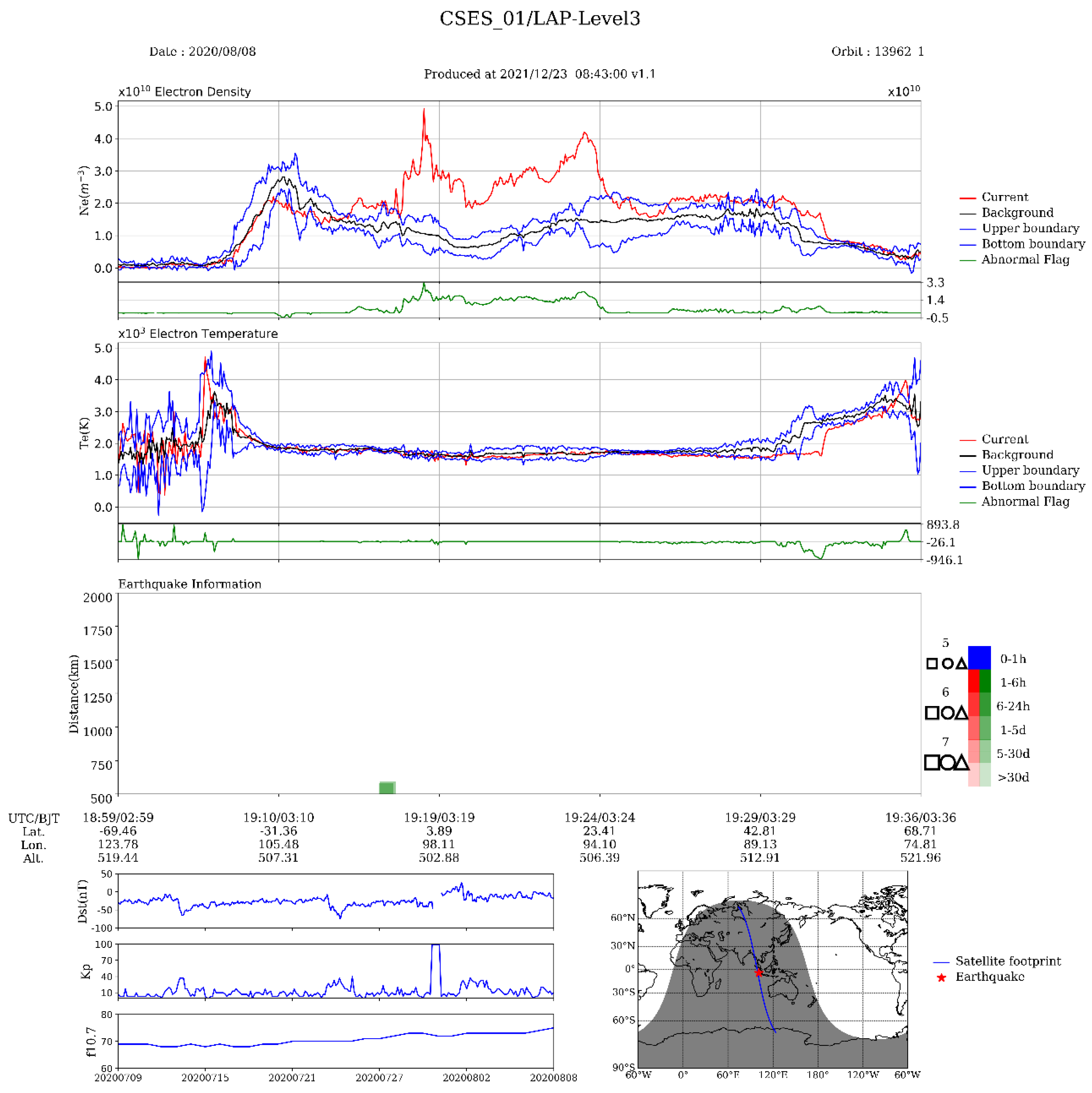
4.1. Single Orbit Analysis

The single orbit analysis is the first step to locate any perturbations recorded by satellites over the EQ influential zone. The physical values (i.e., the power spectral density or amplitude of the electromagnetic field, the density/temperature of plasma parameters, or the flux of energetic particles) recorded by those orbits passing over the EQ influential zone are processed separately as Level 3 data product.
Figure 2 shows an example of the Level 3 data product routinely produced in the CSES scientific application center, which shows the electron density (Ne) and temperature (Te) recorded by orbit No. 13962_1 on 8 August, ten days before the 18 August 2020, M 7.0 Sumatra EQ (see Table 2). The red curves show the observations from the current orbit; the black (average values) and blue (upper and lower boundary) curves present a background trend that is calculated by the revisiting orbits in the previous 30 days (6 orbits in total). It can be seen that the latest Ne data (red) recorded by the current orbit No.13962_1 abnormally increased during the 18 August 2020, M 7.0 Sumatra EQ, significantly exceeding out of the upper (blue) boundary. Considering the space weather conditions (see Figure 3), the enhancement of electron density on 8 August is possibly related to the space weather conditions based on the rough analysis from the Level 3 data product. It is noted that Te data need further validation, not recommended for seismic information analysis directly by using Level 3 data.
The third panel shows the information of EQs that occurred along the current orbit trajectory within one month; the y-axis represents the direct distance between the epicenters and the satellite footpoint; the square, circle, and triangle denote the EQs that occurred before, during, and after the time of the current orbit, respectively; and the EQ magnitude indicates the size of the square, circle, and triangle. The red and green color gradient denote the specific time of EQs that occurred before and after the passing time of the satellite, respectively. The bottom-left figure shows the space weather index (Kp and Dst) within one month (before the date of the current orbit). The bottom-right global map shows the orbit project and the epicenter.
Alternatively, the orbits passing through the epicenter areas are plotted as scatter values of different physical values along the orbit traces, as Figure 2 of Zhima et al. [13], which shows the abnormal enhancement of the power spectral density values in the frequency range from 300 to 800 Hz of the magnetic field.

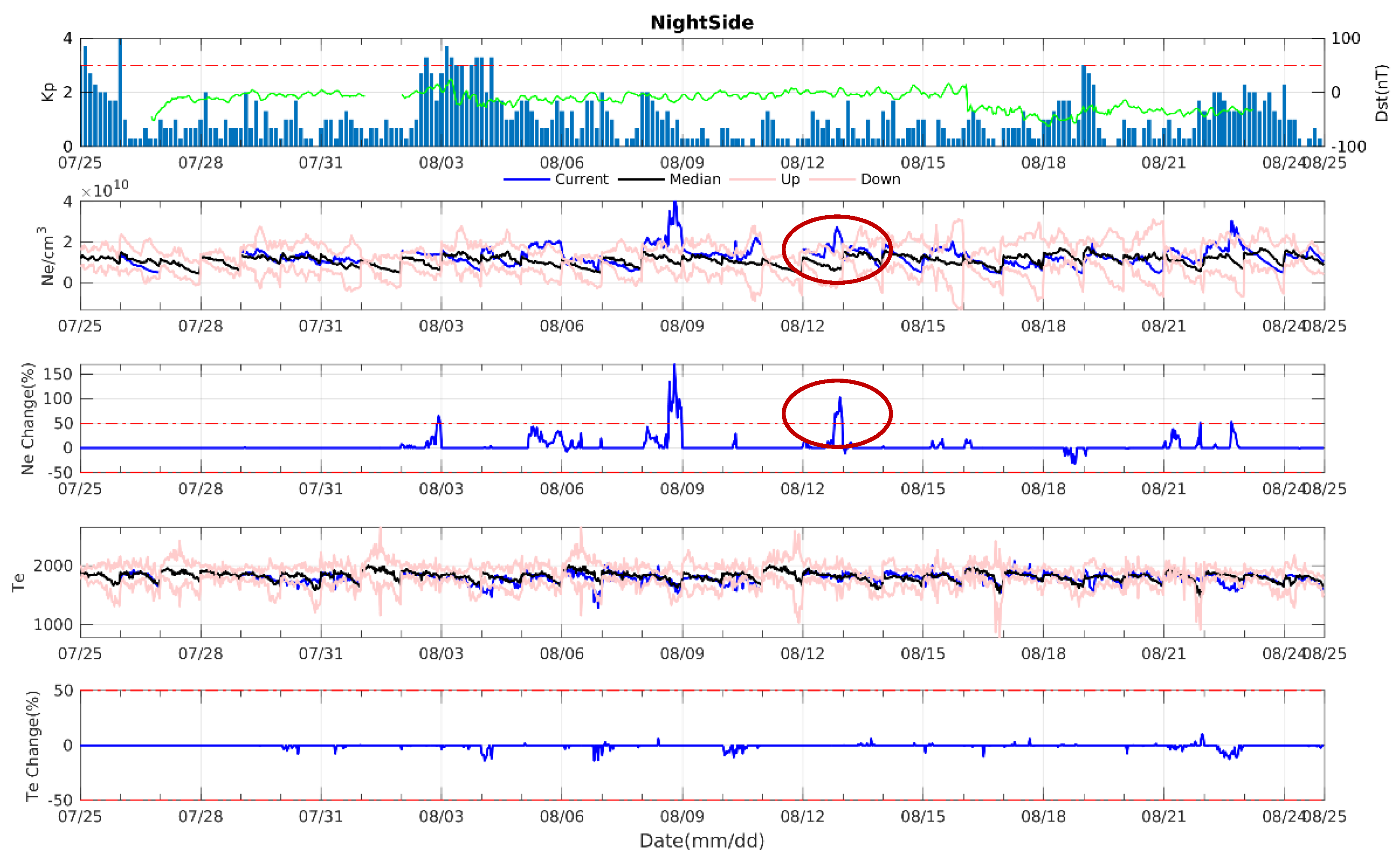
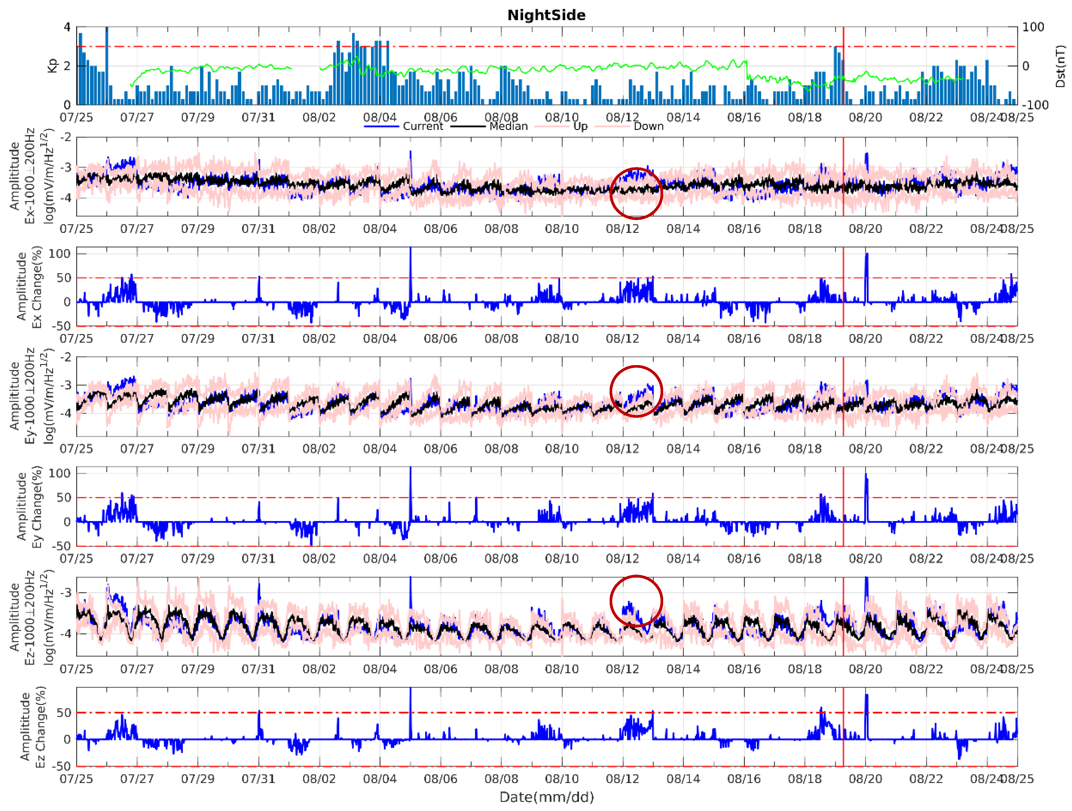
4.2. Multi-Orbits Analysis

After the rough analysis using the Level 3 data products, the second step is to compare the relative long-term observations with the multi-orbits and their revisiting orbits. The physical values over the EQ influential zone from each orbit are extracted and rebuilt as time sequence data. The running quartile method [13,30] is applied to examine the long-term trend. The running medians and the interquartile ranges (i.e., IQR, the difference between the third and first quartiles) were computed using the previous six revisiting orbits (30 days) and the current one (7 orbits in total). The running median values of the time sequence are used to build the background trend, while the median values of the current orbit are regarded as the current observation. The upper and lower bounds are computed by the running median values of physical values ± n*IQR values; n is set from 1 to 5, depending on the different physical quantities. The disturbance amplitude (the difference values between the current observation and the background trend) is normalized as percentages, and if current observation values are within the upper and lower thresholds, the disturbance amplitude is then set to zero.
Figure 3 shows an example of the revisiting orbit analysis, which shows the Ne and Te variation from 25 July to 24 August over the M 7.0 Sumatra epicenter (18 August 2020). From top to bottom are the space weather index (Kp and Dst), the variation in Ne, the disturbance amplitude of Ne, the variation in Te, and the disturbance amplitude of Te. The physical values during the current orbit are plotted as blue curves, and the background median values are plotted as black curves; the upper and lower boundaries are plotted as pink curves. It can be seen that an abnormal increase in Ne appeared on 8 August (10 days); according to the Kp and Dst index, we suggest that it is mainly related to the space weather conditions. The slight increase of 13 August (5 days before the mainshock) appeared under quiet space weather conditions, suggesting that it is possibly linked to the EQ.
Figure 4 shows another example of the electric field, which shows the PSD (power spectral density) values of the Ex, Ey, and Ez components in the frequency range of 1000 Hz ± 100 Hz during the 18 August 2020, M 7.0 Sumatra EQ, in the same format as Figure 3. It can be seen that there was a slight enhancement in the three components of the electric field under the quiet space weather conditions on 13 August, 6 days before the mainshock.
Alternatively, they are plotted in the format of Figure 5, which shows the ULF wave activities in the frequency band from DC to 15 Hz recorded by the revisiting orbits during two Alaska EQs, which occurred on 29 July 2021 (M 8.0) and August 14 (M 7.0) (see Table 2). It is noted that only orbits with abnormal ULF emissions and their revisiting orbits are plotted in Figure 5. Observations on July 28, and August 4 and 7 are removed as there is an apparent AE index enhancement due to the disturbed space weather condition. The variation in the magnetic field intensity along the latitude (−65° to 65°) obtained by the revisiting orbits shows that on 19 July (10 days) and 27 July (2 days) before the 29 July M 8.1 mainshock, the eastward magnetic field in a frequency range from DC to 15 Hz appeared with apparent disturbances. On 10 August (4 days), 12 Auguest (2 days), and 14 August (on the mainshock day) before the 14 August M 7.0 EQ, there were still similar abnormal ULF wave activities. On the other days (some revisiting orbits shown in Figure 4), the strange ULF wave activities were not discovered in the non-EQ activity times over the Alaska epicenter area. It is interesting that the similar but weak ULF emissions also occurred in the southern conjugate point of the epicenter, which is physically possible. The electromagnetic disturbances can propagate along the magnetic field line to the conjugate point of the counterpart hemisphere [10]. Thus, we suggest that the possible abnormal emissions in the ULF band were emitted during the Alaska EQs. However, more evidence is still needed to confirm whether they are linked to the seismic precursors.

4.3. Background Map

The longer-term observations (months or yearly data) under quiet space weather conditions are selected to build a background map. The global background map is built by the median or mean values for specific physical values routinely produced as Level 4 data products for every five days or one year or different seasons (dependent on the types of physical values). The global background map helps depict large-scale ionospheric structures or the electromagnetic field intensity distributions [31,32].
A residual map is built for the specific EQ influential area by the difference values between the background map and the current EQ days (every five days within one month). For example, Figure 6 shows the residual map about the magnetic field in the frequency range from 60 Hz to 70 Hz during the 29 July 2021 and 14 August, M 7.0 Alaska EQs. It is roughly seen from the residual maps that for these two EQs, the PSD values of the magnetic field became enhanced 10 to 5 days before the mainshock (see the map of 20 to 29 July, 4 to 13 August); then, they dropped to a lower level after the mainshock (see the maps of 30 July to 3 August and 14 to 18 August). Admittedly, the residual map always looks disturbed; it is difficult to obtain reliable seismic information most of the time, as shown in Figure 6.

4.4. Multi-Parameter Comparisons

The lithosphere–atmosphere–ionosphere is an open and coupling system; the electromagnetic emissions and the chemistry gases emitted by the stressed rocks in the EQ preparation zones lead to the variation in geophysical and geochemical field, thus directly impacting the ground-based instruments. The seismic signals can also couple into the atmosphere, breaking the chemical reaction balance in there, leading to the formation of local electric currents, air ionization, atmospheric gas condensation, and plasma parameter irregularity [10].
Therefore, in addition to CSES data, the CSES scientific application center also collects multi-source data. At present, the multi-source observations from infrared/hyperspectral remoting sensing satellites, ground-based electromagnetic field instruments, the vertical/oblique ionosonde, and ground-based GNSS receivers etc. can be collected for the first time to comparatively explore the seismic signals with the CSES data.
We pay considerable attention to the atmospheric parameters because the gas released from the crust can effectively change the conductivity condition of the atmosphere, thus leading to a series of coupling processes in the lithosphere–atmosphere–ionosphere [10]. Previous studies have suggested that the atmospheric parameters, such as the radon, methane, aerosol optical depth (AOD), skin temperature (SKT), and surface latent heat flux (SLHF), are sensitive to seismic activities at different stages of the EQ preparation process and can respond sooner to the seismic precursors [33,34] than the seismo-ionospheric parameters. For example, Figure 7 shows the variation in the methane concentration from 2016 to 2021 (provided by the NASA Goddard Earth Sciences Data and Information Services Center) over the Alaska EQ area. Compared with the variation trend from 2016 to 2020, the CH4 concentration increased significantly on 11 July 2021 (18 days before the M 8.1 mainshock), then fell to a low level where the M 8.1 shock occurred; after that, it started to rise to a new peak where the second shock M 7.0 occurred, and the CHR concentration continually decreased and fell back to the background trend level after September 2021.
Figure 8 shows the spatial distribution of the 8 days averaged AOD values (provided by AQUA MODIS C6 of NASA) in 2021 relative to the background field calculated by data from 2001 to 2020 over the Alaska earthquake area. The AOD values became enhanced from 26 June to 21 August, especially in the 8 days time windows of 26 June to 3 July, 28 July to 4 August, and 13 August to 21 August; the AOD is significantly increased relative to the background. The significant enhancements mainly appeared in the southern part of the earthquake epicenter.
The TEC data also easily became disturbed over the forthcoming epicenter regions, showing a significant decrease or increase within one week before the mainshock [35].
Figure 9 shows the vertical TEC anomaly over the Alaska EQs, extracted from the global ionospheric map (GIM) published daily by the International GNSS Service (IGS). The green curve presents the median values of TEC data over the Alaska epicenter zone, and the grey lines are the upper and lower boundaries computed by the IQR method in Section 4.2. The red curve shows the current TEC observations. The red and black bars are the difference values between the red and green curves. It can be seen that the continuous positive anomaly appeared before the July 29 M 8.1 EQ, followed by a negative anomaly after the mainshock. However, it is difficult to identify any apparent anomaly during the August 14, M 7.0 EQ.

5. Discussion

In addition to the single case studies, some statistical studies were also recently carried out using CSES data. For example, Li et al. [16] used the O+ density and electron density data from CSES and the DEMETER satellite to search for seismo-ionospheric perturbations with different time resolutions. The results showed that the detection rate of the seismo-ionospheric disturbance increases as the data time resolution and the earthquake magnitude increase and as the focal depth decreases, proving that the CSES could effectively register seismo-ionospheric perturbations as the DEMETER satellite does [16]. Zhu et al. [36] statistically examined the ~2.5 years of Ne data from CSES during the M 4.8+ EQs worldwide. They found that significant positive Ne variations related to earthquakes mainly occurred ~1 to 7 days and ~13 to 15 days before the earthquakes.
Although numerous independent studies have suggested the seismo-ionospheric disturbances, the earthquake preparation process in the lithosphere and the seismic precursor transport process from the ground to space are still poorly understood due to various variables involved. The pioneering scientists established the Lithosphere–Atmosphere–Ionosphere Coupling (LAIC) models [4,6,10] mainly based on theoretical analyses and observations. Zhao et al. [37] reported a good correlation between CSES’s observation and the full-wave-mode simulation on the VLF radio waves emitted by the ground-based transmitters, confirming the propagation capability of the electromagnetic waves from the lithosphere to the ionosphere. However, due to the complicated seismogenic process and the limited understanding of the seismo-ionospheric phenomena, there are many challenges in the physical process interpretation.
Huang et al. [38] put forward three critical problems in this field: (1) how to perform a reliable and appropriate observation with some precise physical quantities; (2) how to develop a robust methodology to reveal weak earthquake-related electromagnetic signals from the noisy background; and (3) how to develop plausible physical models based on theoretical analyses and/or laboratory experiments for the explanation of the earthquake-related electromagnetic signals observed under the field conditions.
To obtain convincing seismo-ionospheric evidence, we pay considerable attention to data cleaning and data quality control before seismic information extraction. We have performed specific validations on CSES data, and some works about the data quality of the electromagnetic field [37,39,40] and the plasma data [31,41] have been published.
It is admitted that the seismic information analysis methods are still empirical. At present, we interpret data using four methods: the single-orbit analysis, the multi-orbit data analysis, the background map, and the comparative studies with multi-source data recorded from the ground to space. These methods are not sufficient to extract accurate seismic signals. Objectively and correctly extracting the feeble seismic information from the noisy electromagnetic background is still a challenging task, needing a complex multidisciplinary approach to clarify the short-term earthquake precursors by combining the observations at the different altitudes from the lithosphere to the ionosphere [6].

6. Conclusions

This paper briefly introduces the CSES mission, an electromagnetism satellite dedicated to earthquake monitoring using space technology. The routine data preprocessing and seismo-ionospheric information analysis methods are briefly introduced. The possible seismo-ionospheric disturbances that appeared during the strong shallow earthquakes (with a magnitude over 7 and a depth shallower than 30 km) were analyzed by using CSES and other multi-source data.
Based on previous studies and the CSES observations, we suggest that monitoring the short-term precursors from a stereoscopic monitoring system built from the lithosphere-ionosphere is possible. However, it is admitted that there is still a long way to go to identify the seismo-ionospheric precursors from the electromagnetism satellites correctly. Due to the complexity of the EQ preparation mechanism and the limitation of observation technology and data analysis methods, there are many challenges, and we need a multidisciplinary perspective to explore this topic. Finally, we state that the obtained results from the CSES are preliminary, requiring global efforts to search for pre-earthquake short-term precursors using advanced space technology.

Author Contributions

Conceptualization, Z.Z. (Zeren Zhima), J.L., X.S. (Xuhui Shen); Methodology, Z.Z. (Zeren Zhima), R.Y., J.L., Y.Y., Q.W., F.L., J.C., Q.L., S.Z., J.H., Z.Z. (Zhenxia Zhang), S.X., D.L., W.C., H.L.; Software, R.Y., J.L., Y.Y., Q.W., F.L., J.C., Q.L., S.Z., J.H., Z.Z. (Zhenxia Zhang), S.X., D.L., W.C., K.Z., X.S. (Xiaoying Sun), H.L., F.G., Q.T., N.Z.; Validation, Z.Z. (Zeren Zhima); Formal Analysis, Z.Z. (Zeren Zhima), R.Y., J.L., Y.Y., Q.W., J.C., Q.L., S.Z., J.H., Z.Z. (Zhenxia Zhang), S.X., D.L., W.C., H.L.; Investigation, Z.Z. (Zeren Zhima), R.Y., J.L., Y.Y., Q.W., F.L., J.C., Q.L., S.Z., J.H., Z.Z. (Zhenxia Zhang), S.X., D.L., W.C., H.L., D.Y., H.H., J.W.; Resources, X.S. (Xuhui Shen); Data Curation, F.L., K.Z., X.S. (Xiaoying Sun), F.G., Q.T., N.Z.; Writing—Original Draft, Z.Z. (Zeren Zhima), Y.Y.; Writing—Review & Editing, Z.Z. (Zeren Zhima); Visualization, R.Y., Y.Y., Q.W., F.L., J.C., Q.L., S.Z., J.H., Z.Z. (Zhenxia Zhang), S.X., D.L., W.C., K.Z., X.S. (Xiaoying Sun), H.L.; Supervision, J.L., X.S. (Xuhui Shen); Project Administration, X.S. (Xuhui Shen); Funding Acquisition, Z.Z. (Zeren Zhima), X.S. (Xuhui Shen). All authors have read and agreed to the published version of the manuscript.

Funding

This work is supported by the NSFC Grant 41874174/41574139, National Key R&D Program of China (Grant No.2018YFC1503501), the APSCO Earthquake Research Project Phase II, ISSI-BJ project, and Dragon project phase five.

Institutional Review Board Statement

Not applicable.

Informed Consent Statement

Not applicable.

Data Availability Statement

The data of CSES can be downloaded from the website (http://www.leos.ac.cn/ accessed on 26 December 2021). The solar wind parameters and geomagnetic Kp and Dst indices are provided by the World Data Center for Geomagnetism, Kyoto (http://wdc.kugi.kyoto-u.ac.jp/ accessed on 26 December 2021). The earthquake catalog is provided by China Earthquake Networks Center (http://www.ceic.ac.cn/dataout accessed on 26 December 2021). The ground-based TEC data are extracted from the global ionospheric map (GIM) published daily by the International GNSS Service (IGS). The atmospheric data are provided by the website https://disc.gsfc.nasa.gov/datasets/ (accessed on 26 December 2021).

Acknowledgments

This work is a joint endeavor of the CSES team to monitor earthquake activities using advanced space technology. We acknowledge all the CSES team members and those who support the CSES mission.

Conflicts of Interest

The authors declare no conflict of interest.

References

  1. King, C.-Y. Earthquake prediction: Electromagnetic emissions before earthquakes. Nature 1983, 301, 377. [Google Scholar] [CrossRef]
  2. Gokhberg, M.B.; Morgounov, V.A.; Yoshino, T.; Tomizawa, I. Experimental measurement of electromagnetic emissions possibly related to earthquakes in Japan. J. Geophys. Res. 1982, 87, 7824. [Google Scholar] [CrossRef]
  3. Nestorov, G. A possible ionospheric presage of the Vrancha earthquake of March 4, 1977. Bolgarska Akademiia Nauk Doklady 1979, 32, 443–446. [Google Scholar]
  4. Hayakawa, M. Probing the lower ionospheric perturbations associated with earthquakes by means of subionospheric VLF/LF propagation. Earthq. Sci. 2011, 24, 609–637. [Google Scholar] [CrossRef] [Green Version]
  5. Ouzounov, D.; Pulinets, S.; Hattori, K.; Taylor, P. Pre-Earthquake Processes: A Multidisciplinary Approach to Earthquake Prediction Studies; John Wiley & Sons: Hoboken, NJ, USA, 2018; Volume 234. [Google Scholar]
  6. Pulinets, S.; Ouzounov, D. Lithosphere–Atmosphere–Ionosphere Coupling (LAIC) model–An unified concept for earthquake precursors validation. J. Asian Earth Sci. 2011, 41, 371–382. [Google Scholar] [CrossRef]
  7. Larkina, V.I.; Migulin, V.V.; Molchanov, O.A.; Kharkov, I.P.; Inchin, A.S.; Schvetcova, V.B. Some statistical results on very low frequency radiowave emissions in the upper ionosphere over earthquake zones. Phys. Earth Planet. Inter. 1989, 57, 100–109. [Google Scholar] [CrossRef]
  8. Parrot, M. VLF emissions associated with earthquakes and observed in the ionosphere and the magnetosphere. Phys. Earth Planet. Inter. 1989, 57, 86–99. [Google Scholar] [CrossRef]
  9. Chmyrev, V.; Isaev, N.; Bilichenko, S.; Stanev, G. Observation by space-borne detectors of electric fields and hydromagnetic waves in the ionosphere over an earthquake centre. Phys. Earth Planet. Inter. 1989, 57, 110–114. [Google Scholar] [CrossRef]
  10. Pulinets, S.; Ouzounov, D. The Possibility of Earthquake Forecasting; IOP Publishing: Bristol, UK, 2018. [Google Scholar]
  11. Parrot, M.; Berthelier, J.; Lebreton, J.; Sauvaud, J.; Santolik, O.; Blecki, J. Examples of unusual ionospheric observations made by the DEMETER satellite over seismic regions. Phys. Chem. Earth Parts A/B/C 2006, 31, 486–495. [Google Scholar] [CrossRef]
  12. Zhima, Z.; Xuhui, S.; Xuemin, Z.; Jinbin, C.; Jianping, H.; Xinyan, O.; Jing, L.; Lu, B. Possible ionospheric electromagnetic perturbations induced by the Ms7. 1 Yushu earthquake. Earth Moon Planets 2012, 108, 231–241. [Google Scholar] [CrossRef]
  13. Zhima, Z.; Hu, Y.; Pierstanti, M.; Shen, X.; De Santis, A.; Yan, R.; Yang, Y.; Zhao, S.; Zhang, Z.; Wang, Q. The seismic electromagnetic emissions during the 2010 Mw 7.8 Northern Sumatra Earthquake revealed by DEMETER satellite. Front. Earth Sci. 2020, 8, 459. [Google Scholar] [CrossRef]
  14. Nemec, F.; Santolík, O.; Parrot, M. Decrease of intensity of ELF/VLF waves observed in the upper ionosphere close to earthquakes: A statistical study. J. Geophys. Res. 2009, 114, A04303. [Google Scholar] [CrossRef]
  15. Zhao, B.; Wang, M.; Yu, T.; Wan, W.; Lei, J.; Liu, L.; Ning, B. Is an unusual large enhancement of ionospheric electron density linked with the 2008 great Wenchuan earthquake? J. Geophys. Res. Space Phys. 2008, 113, A11304. [Google Scholar] [CrossRef]
  16. Li, M.; Shen, X.; Parrot, M.; Zhang, X.; Zhang, Y.; Yu, C.; Yan, R.; Liu, D.; Lu, H.; Guo, F. Primary joint statistical seismic influence on ionospheric parameters recorded by the CSES and DEMETER satellites. J. Geophys. Res. Space Phys. 2020, 125, e2020JA028116. [Google Scholar] [CrossRef]
  17. Pulinets, S.; Legen’ka, A.D. Spatial-temporal characteristics of the large scale disturbances of electron concentration observed in the F-region of the ionosphere before strong earthquakes. Cosm. Res. 2003, 41, 221–229. [Google Scholar] [CrossRef]
  18. Marchetti, D.; De Santis, A.; D’Arcangelo, S.; Poggio, F.; Jin, S.; Piscini, A.; Campuzano, S.A. Magnetic field and electron density anomalies from Swarm satellites preceding the major earthquakes of the 2016–2017 Amatrice-Norcia (Central Italy) seismic sequence. Pure Appl. Geophys. 2020, 177, 305–319. [Google Scholar] [CrossRef]
  19. Shen, X.; Zhang, X.; Yuan, S.; Wang, L.; Cao, J.; Huang, J.; Zhu, X.; Picozzo, P.; Dai, J. The state-of-the-art of the China Seismo-Electromagnetic Satellite mission. Sci. China Technol. Sci. 2018, 61, 634–642. [Google Scholar] [CrossRef]
  20. Zhou, B.; Yang, Y.; Zhang, Y.; Gou, X.; Cheng, B.; Wang, J.; Li, L. Magnetic field data processing methods of the China Seismo-Electromagnetic Satellite. Earth Planet. Phys. 2018, 2, 455–461. [Google Scholar] [CrossRef]
  21. Pollinger, A.; Lammegger, R.; Magnes, W.; Hagen, C.; Ellmeier, M.; Jernej, I.; Leichtfried, M.; Kürbisch, C.; Maierhofer, R.; Wallner, R.; et al. Coupled dark state magnetometer for the China Seismo-Electromagnetic Satellite. Meas. Sci. Technol. 2018, 29, 095103. [Google Scholar] [CrossRef] [Green Version]
  22. Cao, J.; Zeng, L.; Zhan, F.; Wang, Z.; Wang, Y.; Chen, Y.; Meng, Q.; Ji, Z.; Wang, P.; Liu, Z.; et al. The electromagnetic wave experiment for CSES mission: Search coil magnetometer. Sci. China Technol. Sci. 2018, 61, 653–658. [Google Scholar] [CrossRef]
  23. Huang, J.; Lei, J.; Li, S.; Zeren, Z.; Li, C.; Zhu, X.; Yu, W. The Electric Field Detector (EFD) onboard the ZH-1 satellite and first observational results. Earth Planet. Phys. 2018, 2, 469–478. [Google Scholar] [CrossRef]
  24. Liu, C.; Guan, Y.; Zheng, X.; Zhang, A.; Piero, D.; Sun, Y. The technology of space plasma in-situ measurement on the China Seismo-Electromagnetic Satellite. Sci. China Technol. Sci. 2019, 62, 829–838. [Google Scholar] [CrossRef]
  25. Lin, J.; Shen, X.; Hu, L.; Wang, L.; Zhu, F. CSES GNSS ionospheric inversion technique, validation and error analysis. Sci. China Technol. Sci. 2018, 61, 669. [Google Scholar] [CrossRef]
  26. Li, X.Q.; Xu, Y.B.; An, Z.H.; Liang, X.H.; Wang, P.; Zhao, X.Y.; Wang, H.Y.; Lu, H.; Ma, Y.Q.; Shen, X.H.; et al. The high-energy particle package onboard CSES. Radiat. Detect. Technol. Methods 2019, 3, 22. [Google Scholar] [CrossRef]
  27. Picozza, P.; Battiston, R.; Ambrosi, G.; Bartocci, S.; Basara, L.; Burger, W.J.; Campana, D.; Carfora, L.; Casolino, M.; Castellini, G.; et al. Scientific Goals and In-orbit Performance of the High-energy Particle Detector on Board the CSES. Astrophys. J. Suppl. Ser. 2019, 243, 16. [Google Scholar] [CrossRef]
  28. Dobrovolsky, I.P.; Zubkov, S.I.; Miachkin, V.I. Estimation of the size of earthquake preparation zones. Pure Appl. Geophys. 1979, 117, 1025–1044. [Google Scholar] [CrossRef]
  29. Parrot, M. Statistical study of ELF/VLF emissions recorded by a low-altitude satellite during seismic events. J. Geophys. Res. 1994, 99, 23339–23347. [Google Scholar] [CrossRef]
  30. Liu, J.Y.; Chen, Y.I.; Chuo, Y.J.; Chen, C.S. A statistical investigation of preearthquake ionospheric anomaly. J. Geophys. Res. Space Phys. 2006, 111, 61–65. [Google Scholar] [CrossRef] [Green Version]
  31. Yan, R.; Zhima, Z.; Xiong, C.; Shen, X.; Huang, J.; Guan, Y.; Zhu, X.; Liu, C. Comparison of Electron Density and Temperature from the CSES Satellite With Other Space-Borne and Ground-Based Observations. J. Geophys. Res. Space Phys. 2020, 125, e2019JA027747. [Google Scholar] [CrossRef]
  32. Zhima, Z.; Hu, Y.; Shen, X.; Chu, W.; Piersanti, M.; Parmentier, A.; Zhang, Z.; Wang, Q.; Huang, J.; Zhao, S.; et al. Storm-Time Features of the Ionospheric ELF/VLF Waves and Energetic Electron Fluxes Revealed by the China Seismo-Electromagnetic Satellite. Appl. Sci. 2021, 11, 2617. [Google Scholar] [CrossRef]
  33. Cui, J.; Shen, X.; Zhang, J.; Ma, W.; Chu, W. Analysis of spatiotemporal variations in middle-tropospheric to upper-tropospheric methane during the Wenchuan M s = 8.0 earthquake by three indices. Nat. Hazards Earth Syst. Sci. 2019, 19, 2841–2854. [Google Scholar] [CrossRef] [Green Version]
  34. Liu, Q.; De Santis, A.; Piscini, A.; Cianchini, G.; Ventura, G.; Shen, X. Multi-parametric climatological analysis reveals the involvement of fluids in the preparation phase of the 2008 Ms 8.0 wenchuan and 2013 Ms 7.0 lushan earthquakes. Remote Sens. 2020, 12, 1663. [Google Scholar] [CrossRef]
  35. Liu, J.Y.; Chen, Y.I.; Chen, C.H.; Liu, C.Y.; Chen, C.Y.; Nishihashi, M.; Li, J.Z.; Xia, Y.Q.; Oyama, K.I.; Hattori, K.; et al. Seismoionospheric GPS total electron content anomalies observed before the May 12 2008 Mw7.9 Wenchuan earthquake. J. Geophys. Res. 2009, 114, A04320. [Google Scholar] [CrossRef]
  36. Zhu, K.; Zheng, L.; Yan, R.; Shen, X.; Zeren, Z.; Xu, S.; Chu, W.; Liu, D.; Zhou, N.; Guo, F. Statistical study on the variations of electron density and temperature related to seismic activities observed by CSES. Nat. Hazards Res. 2021, 1, 88–94. [Google Scholar] [CrossRef]
  37. Zhao, S.; Zhou, C.; Shen, X.; Zhima, Z. Investigation of VLF Transmitter Signals in the Ionosphere by ZH-1 Observations and Full-Wave Simulation. J. Geophys. Res. Space Phys. 2019, 124, 4697–4709. [Google Scholar] [CrossRef]
  38. Huang, Q.; Han, P.; Hattori, K.; Ren, H. Electromagnetic Signals Associated with Earthquakes. In Seismoelectric Exploration; Wiley: Hoboken, NJ, USA, 2020; pp. 415–436. [Google Scholar]
  39. Zhima, Z.; Zhou, B.; Zhao, S.; Wang, Q.; Huang, J.; Zeng, L.; Chen, J.L.Y.; Li, C.; Yang, D.; Sun, X.; et al. Cross-calibration on the electromagnetic field detection payloads of the China Seismo-Electromagnetic Satellite. Sci. China Technol. Sci. 2022, 18. [Google Scholar]
  40. Yang, Y.; Zhou, B.; Hulot, G.; Olsen, N.; Wu, Y.; Xiong, C.; Stolle, C.; Zhima, Z.; Huang, J.; Zhu, X. CSES high precision magnetometer data products and example study of an intense geomagnetic storm. J. Geophys. Res. Space Phys. 2021, 126, e2020JA028026. [Google Scholar] [CrossRef]
  41. Yan, R.; Guan, Y.; Miao, Y.; Zhima, Z.; Xiong, C.; Zhu, X.; Liu, C.; Shen, X.; Yuan, S.; Liu, D. The regular features recorded by the Langmuir probe onboard the low earth polar orbit satellite CSES. J. Geophys. Res. Space Phys. 2022, 127, e2021JA029289. [Google Scholar] [CrossRef]
Figure 1. The global earthquake activity occurred after the launch of CSES in February 2018 to 1 December 2021. The overlapping black lines are the orbit trajectories of the CSES.
Remotesensing 14 00905 g001
Figure 2. The typical Level 3 data automatically produced in the CSES scientific application center, taking the example of electron density observation from orbit No. 13962-1 on 8 August, ten days before the 18 August 2020, M 7.0 Sumatra EQ. See text for details about the meaning of each plot and displayed variables.
Remotesensing 14 00905 g002
Figure 3. The electron density disturbances over the 18 August 2020, M 7.0 Sumatra EQ influential area. The space weather index Kp is presented by blue bars, and the Dst index is displayed by the cyan curve. The red horizontal dashed line represents the values of Kp = 3.
Remotesensing 14 00905 g003
Figure 4. The electric field variation in frequency at 1000 ± 100 Hz during 18 August 2020, M 7.0 Sumatra EQ. The space weather index Kp is presented by blue bars, and the Dst index is displayed by the cyan curve. The red horizontal dashed line represents the values of Kp = 3.
Remotesensing 14 00905 g004
Figure 5. The abnormal ULF waves emitted before the 2021 M 8.1 and M 7.0 EQs in Alaska.
Remotesensing 14 00905 g005
Figure 6. The magnetic field disturbances in frequency from 60 to 73 Hz relative to the background map revealed by the PSD values of the variant magnetic field recorded by SCM during the 29 July 2021 M 8.1 and August 14 M 7.0 Alaska EQs. The star denotes the epicenter location.
Remotesensing 14 00905 g006
Figure 7. The CH4 volume mixing ratio value (VMR) variation over the 29 July 2021 M 8.1 and 14 August M 7.0 Alaska EQs.
Remotesensing 14 00905 g007
Figure 8. The variation in 8 days averaged AOD during the EQ time after removal of the background, which is built by AOD values from 2001–2021 over the Alaska epicenters. The star denotes the epicenter location.
Remotesensing 14 00905 g008
Figure 9. The variation in VTEC over the 29 July 2021 M 8.1 and August 14 M 7.0 Alaska epicenters.
Remotesensing 14 00905 g009
Table 1. The scientific payloads onboard CSES.
Detection ObjectivesPayloadsParameters
The geomagnetic field High-Precision Magnetometer (HPM)Including two tri-axial fluxgate magnetometers (FGMs) and one coupled dark-state magnetometer (CDSM)
Detection band: DC to 15 Hz
The vector and scalar values
The electromagnetic fieldSearch-Coil Magnetometer (SCM) The waveform or power spectral density values in the three frequency bands:
ULF: 10 Hz–200 Hz, sampling rate 1024 Hz
ELF: 200 Hz–2200 Hz, sampling rate 10.24 kHz,
VLF: 1.8 kHz–20 kHz, sampling rate 50 kHz
Electric field detector (EFD)The waveform or power spectral density values in the four frequency bands:
ULF: DC–16 Hz, sampling rate 128 Hz,
ELF: 6 Hz–2.2 kHz, sampling rate 5 kHz
VLF: 1.8 kHz–20 kHz, sampling rate 51.2 kHz
HF: 18 kHz–3.5 MHz, sampling rate 10 MHz.
The in situ ionospheric parametersPlasma analyzer package (PAP)Ion density, ion temperature, ion contents (H+, O+, He+)
Ion drift velocity (Vx, Vy, Vz)
Langmuir probe (LAP)Electron density/temperature, the plasma/the satellite floating potential
The profile ionospheric parametersGNSS Occultation Receiver (GOR) TEC, Ne profile, the profile of air temperature and pressure, HmF2, NmF2
Tri-Band Beacon (TBB)Three bands: 50/400/1066 MHz,
Physical values: relative TEC, Ne Profile, ionospheric scintillation index, and ionosphere tomography
The energetic particlesEnergetic particle detector
(HEPP), including three detectors, HEPP-H, HEPP-L, and HEPP-X.
HEPP-L: Electron: 0.1–3 MeV, Proton: 2–20 MeV
HEPP-H: Electron: 1.5–50 MeV, Proton: 2–20 MeV
HEPP-X: Solar X-ray: 0.9–35 keV
Italian Energetic particle detector (HEPD)Proton flux: 30–100 MeV
Electron flux: 30–200 MeV
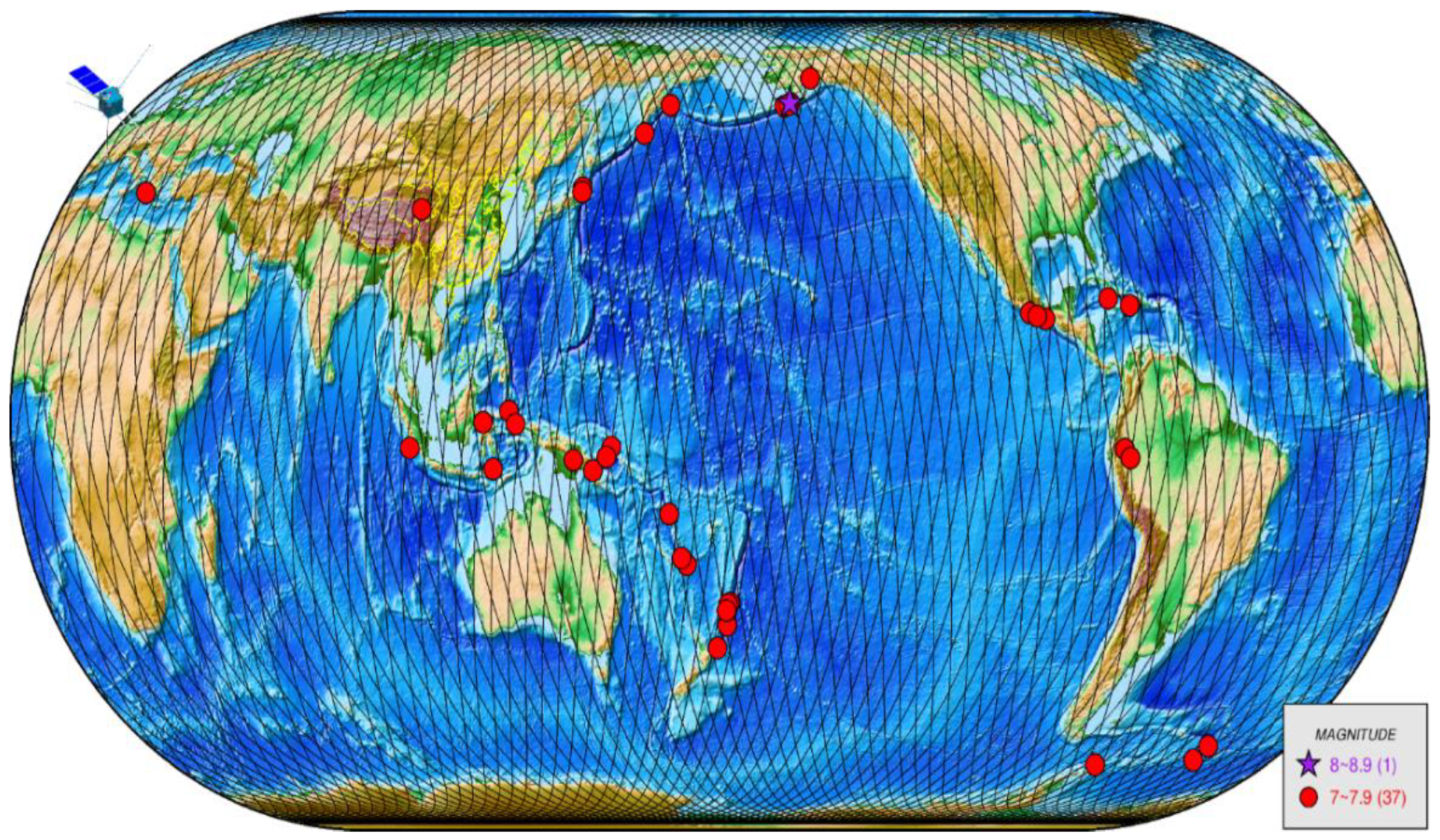
Table 2. The possible seismo-ionospheric disturbances recorded by the CSES during the shallow strong EQs.
No.Place UTCLatitude (°)Longitude (°)Magnitude (M) Depth (km)The Possible Seismo-Ionospheric Perturbation
1Mexico16 February 2018 23:39:3816.6−97.757.110The abnormal emissions at frequencies 155.5 Hz and 1.405 kHz.
The electron density and ion (O+) density increased two days before the mainshock.
2Papua New Guinea25 February 2018 17:44:42−6.19142.777.520The magnetic field enhancement at the frequency of 155 Hz nearest the epicenter 7 and 3 days before the mainshock.
The electron/ion disturbed 7, 6, 5, and 2 days before the mainshock.
3Loyalty Islands Region 29 August 2018 03:51:54−21.95170.17.120The electron density increased; the PSD values of the electromagnetic field at the ELF frequency increased; the energetic particle flux within 0.1–3 MeV increased during the mainshock.
4Indonesia28 September 2018 10:02:44−0.25119.97.410The electron density significantly increased 12 and 2 days before the mainshock.
5Papua New Guinea10 October 2018 20:48:18−5.70151.257.120The abnormal emissions at ULF/ELF/VLF frequencies 9 and 4 days before the mainshock.
The electron density and energetic particle flux disturbed 5 and 2 days before and on the mainshock day.
6Kmadek islands, New Zealand15 June 2019 22:55:00−30.80−178.107.220The in situ and occultation electron density abnormally increased within one week before the mainshock.
7Southern waters of Cuba 28 Janarury 2020 19:10:2219.46−78.797.710The electron density increased over the conjugate area on January 27 and the epicenter area on January 28.
8Mexico 23 June 2020 15:29:0416.14−95.757.410The electron density became disturbed 3 days before the mainshock.
9Sumatra island, Indonesia 18 August 2020 22:29:21−4.31101.157.010The electron density significantly increased 10 days before the mainshock.
10Maduo County, Qinghai, China21 May 2021 18:04:1134.5998.347.417The electron density and the electromagnetic field in the ULF/ELF band observed a simultaneous increase 8 days before the mainshock.
Energetic electrons at energy levels 0.1 to 3 MeV increased 7 days and 6 days before the mainshock.
The electric field intensity in the VLF band increased one day before the mainshock.
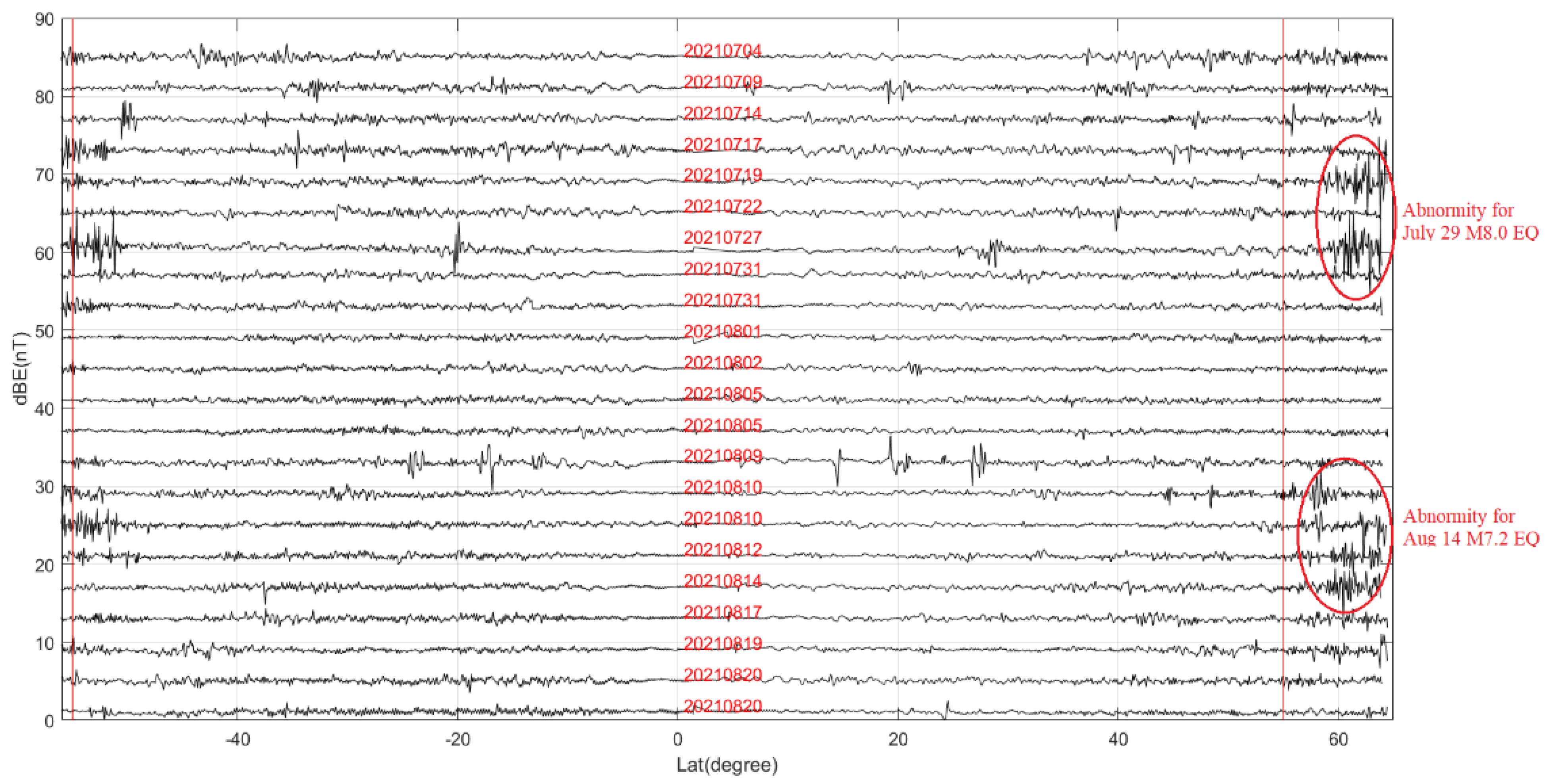
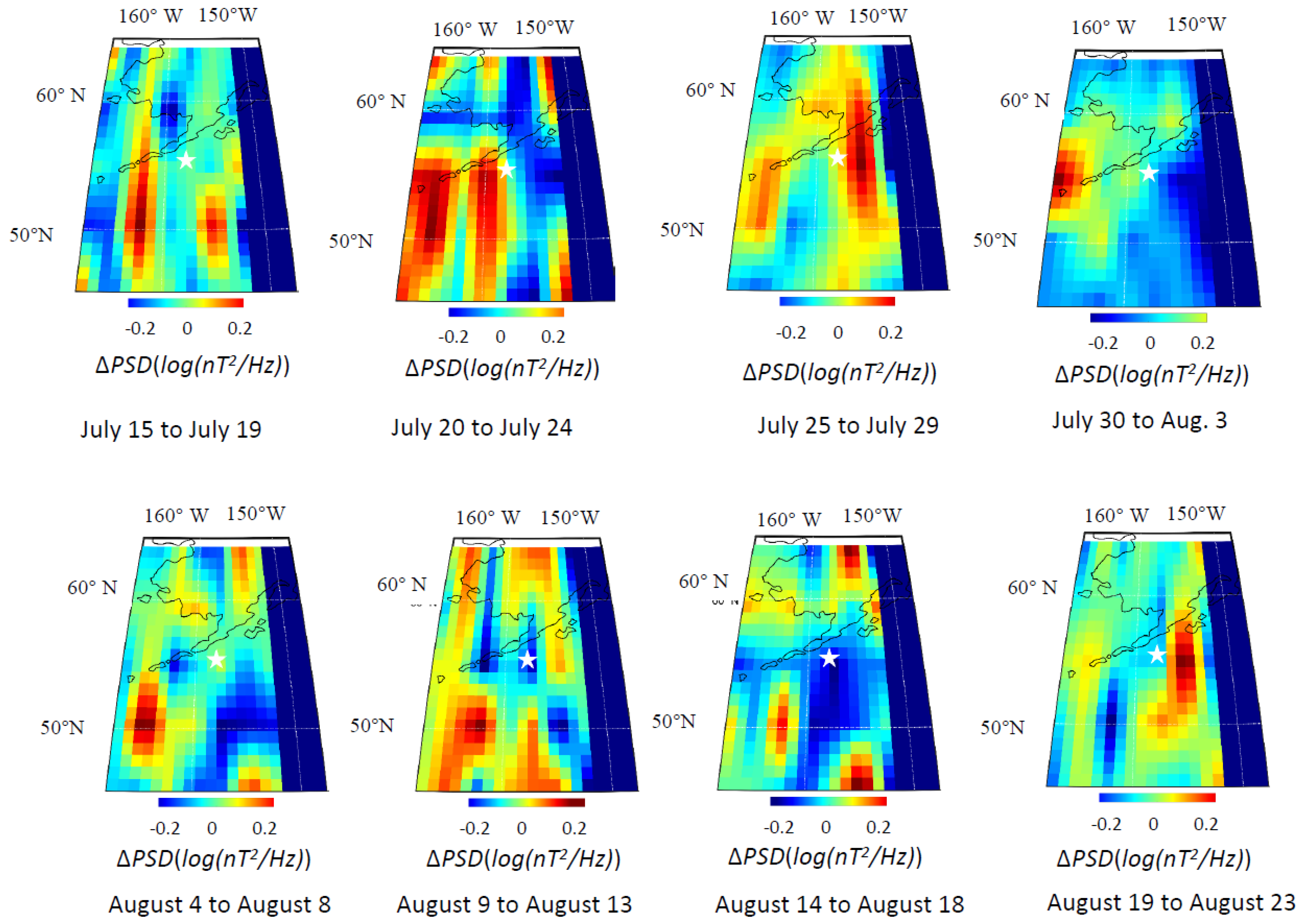
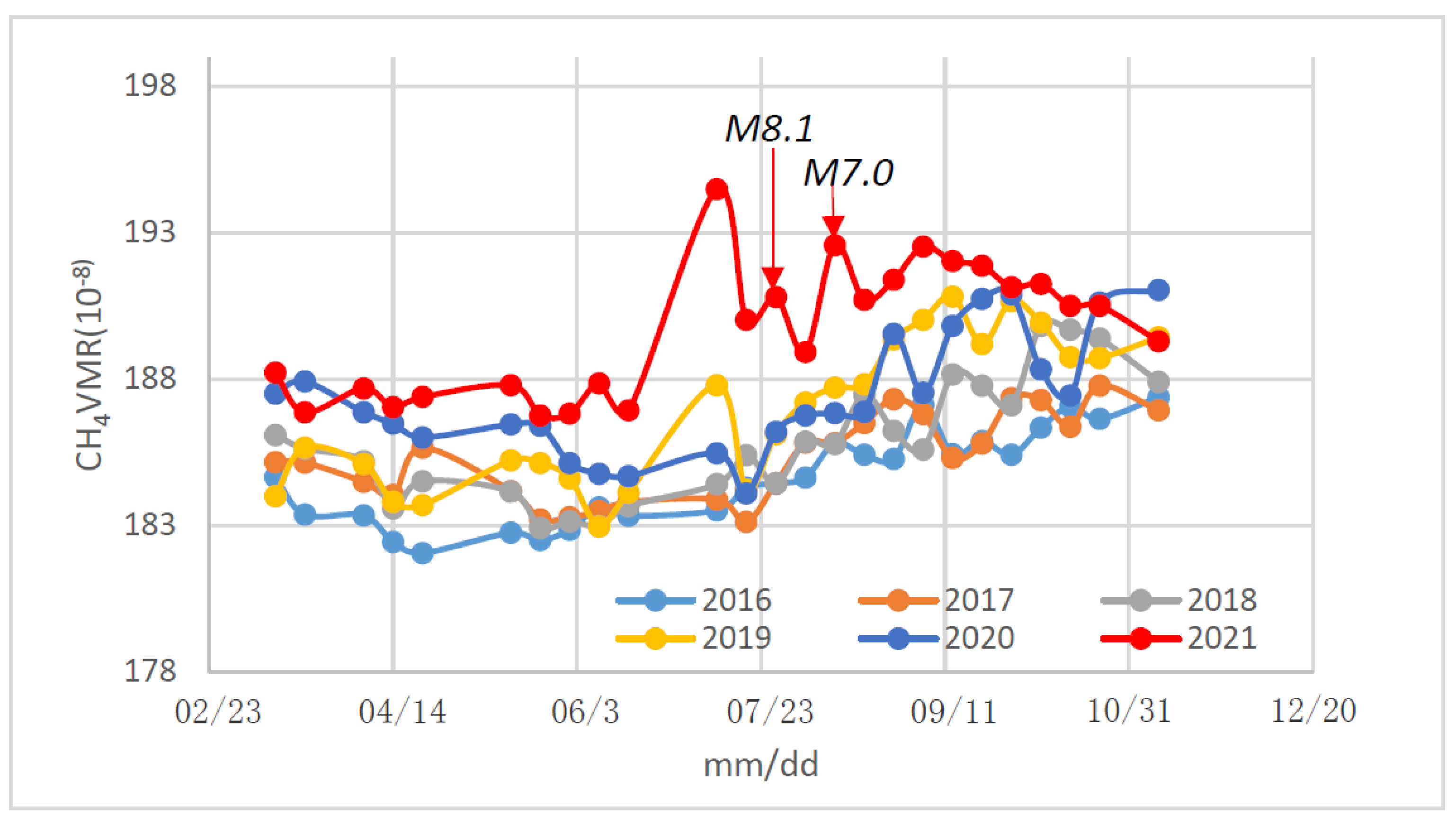
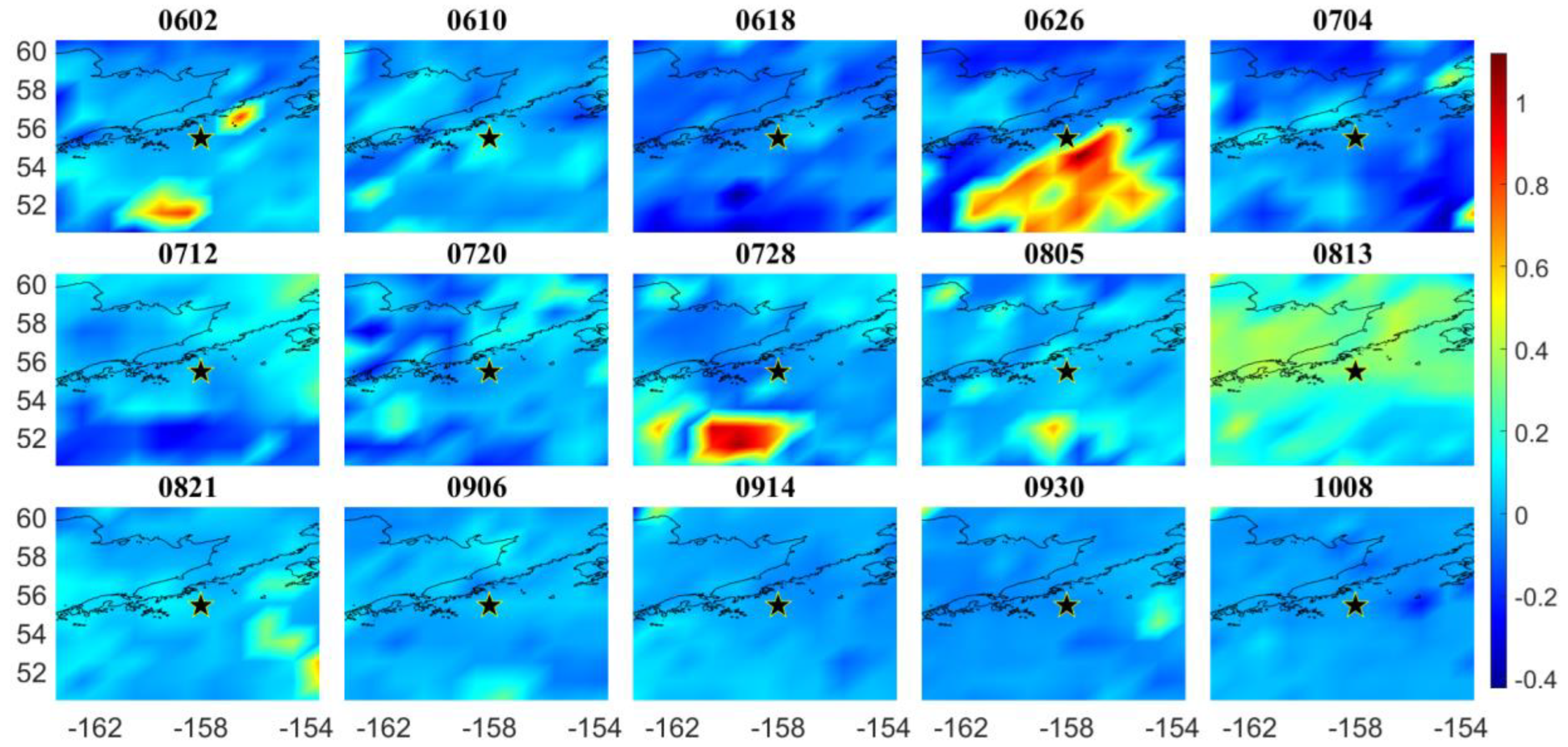
11Near Alaska Peninsula 29 July 2021 06:15:4655.40−158.008.110An abnormal ULF wave appeared 10 and 2 days before the mainshock.
The infrared hyperspectral methane, OLR, aerosol, and other long-term observation data observed anomalies more than a month before the earthquake.
12South water of Alaska 14 August 2021 11:57:4255.30−157.757.010The abnormal ULF emissions occurred 12 and 4 days before and on the mainshock day.
13Haiti region 14 August 2021 12:29:0718.35−73.457.310The electromagnetic field intensity in the ULF/ELF band increased on 4 days, and one day before the mainshock.
The energetic particle flux from 100 to 200 keV increased 4 and 3 days before the mainshock.
Publisher’s Note: MDPI stays neutral with regard to jurisdictional claims in published maps and institutional affiliations.

