Article

Assessing Surface Water Losses and Gains under Rapid Urbanization for SDG 6.6.1 Using Long-Term Landsat Imagery in the Guangdong-Hong Kong-Macao Greater Bay Area, China

1
Beijing Key Laboratory for Remote Sensing of Environment and Digital Cities, Faculty of Geographical Science, Beijing Normal University, Beijing 100875, China
2
State Key Laboratory of Remote Sensing Science, Faculty of Geographical Science, Beijing Normal University, Beijing 100875, China
3
School of Geographical Science, Guangzhou University, Guangzhou 510006, China
4
School of Geography and Planning, Nanning Normal University, Nanning 530001, China
5
School of Architecture and Civil Engineering, Chengdu University, Chengdu 610106, China
*
Author to whom correspondence should be addressed.
Remote Sens. 2022, 14(4), 881; https://doi.org/10.3390/rs14040881
Submission received: 16 December 2021 / Revised: 23 January 2022 / Accepted: 10 February 2022 / Published: 12 February 2022
(This article belongs to the Special Issue Remote Sensing of Wetlands and Biodiversity)

Abstract

:
As one of the most open and dynamic regions in China, the Guangdong-Hong Kong-Macao Greater Bay Area (GBA) has been urbanizing rapidly in recent decades. The surface water in the GBA also has been suffering from urbanization and intensified human activities. The study aimed to characterize the spatiotemporal patterns and assess the losses and gains of surface water caused by urbanization in the GBA via long time-series remote sensing data, which could support the progress towards sustainable development goals (SDGs) set by the United Nations, especially for measuring SDG 6.6.1 indicator. Firstly, utilizing 4750 continuous Landsat TM/ETM+/OLI images during 1986–2020 and the Google Earth Engine cloud platform, the multiple index water detection rule (MIWDR) was performed to extract surface water extent in the GBA. Secondly, we achieved surface water dynamic type classification based on annual water inundation frequency time-series in the GBA. Finally, the spatial distribution and temporal variation of urbanization-induced water losses and gains were analyzed through a land cover transfer matrix. Results showed that (1) the average minimal and maximal surface water extents of the GBA during 1986–2020 were 2017.62 km2 and 6129.55 km2, respectively. The maximal surface water extent fell rapidly from 7897.96 km2 in 2001 to 5087.46 km2 in 2020, with a loss speed of 155.41 km2 per year (R2 = 0.86). (2) The surface water areas of permanent and dynamic types were 1529.02 km2 and 2064.99 km2 during 2000–2020, accounting for 42.54% and 57.46% of all water-related areas, respectively. (3) The surface water extent occupied by impervious land surfaces showed a significant linear downward trend (R2 = 0.98, slope = 36.41 km2 per year), while the surface water restored from impervious land surfaces denoted a slight growing trend (R2 = 0.86, slope = 0.99 km2 per year). Our study monitored the long-term changes in the surface water of the GBA, which can provide valuable information for the sustainable development of the GBA urban agglomeration. In addition, the proposed framework can easily be implemented in other similar regions worldwide.

1. Introduction

Terrestrial surface water bodies, which include lakes, rivers, reservoirs, ponds and partially impounded farmland, are a critically important component of water resources for human life and terrestrial ecosystems [1]. Surface water provides and supports diverse ecosystem services for human activities and natural habitats [2].
However, over the past 30 years, the global permanent water area has decreased by 90,000 km2 due to human activities and climate change [3]. It is necessary to monitor surface water dynamics to inform water resources protection and regional sustainable development. Among the Sustainable Development Goals (SDGs) proposed by the United Nations in 2015, SDG 6.6.1, which measures “the spatial extent of water-related ecosystem”, aims to track changes in different types of water-related ecosystems to support the recovery of already degraded water-related ecosystems and prevent surface water degradation [4,5]. Hence, SDG 6.6.1 is closely related to the monitoring of water-related ecosystems. As in the previous studies of Fitoka et al. and Weise et al., spatial mapping methods of wetlands were developed and their research results were applied to the analysis of SDG 6.6.1 [6,7].
Remote sensing technology can be employed to monitor the spatiotemporal dynamics of surface water bodies in a more large-scale, refined, accurate and fast manner [8,9,10,11] compared with conventional spatial measurement and statistic methods [12], as well as to better serve the goal of realizing SDG 6.6.1. In the era of remote sensing big data, monitoring surface water dynamics on a large spatial scale with long time series remote sensing images has become the focus of numerous studies [13,14,15,16]. Furthermore, the Google Earth Engine (GEE) Cloud Platform is widely applied to process massive remote sensing data [17] quickly and efficiently, especially for large-scale and long time-series studies [18,19]. Studies, such as those of Wang et al. (2018, 2019 and 2021), Zhou et al., and Li et al., achieved water extraction through the GEE platform and analyzed surface water dynamics at large and regional spatial scales [20,21,22,23]. Additionally, the remote sensing data and GEE platform were also utilized to monitor the dynamics of Dongting lake and Baiyangdian lake for reporting SDG 6.6.1, as put forward in the study of Jiang et al. [2] and Wang et al. [21].
At present, the widely used water extraction methods based on remote sensing include the water extraction index, single-band and multiband methods, machine learning methods [24,25,26,27,28], and so on. Among them, the water body extraction index method has the advantages of high efficiency and reliable accuracy [29]. Currently, plenty of water body extraction indices have been proposed to extract water extent. The most popular water body extraction indices include the normalized difference water index (NDWI) [30,31], modified normalized difference water index (MNDWI) [32] and automated water extraction index (AWEI) [33]. These water extraction indices have simple calculation equations and high accuracy, but they also have their corresponding shortages. Combining the advantages of different water indices has proven to be a reasonable solution to this issue [26].
The GBA is one of the most open economically dynamic regions in China and plays a crucial strategic role in China’s overall development. Released in February 2019, the central government issued the Outline of the Development Plan for the Guangdong-Hong Kong-Macao Greater Bay Area (http://www.cnbayarea.org.cn, accessed on 17 June 2021), which aims to connect nine cities in the Pearl River Delta of Guangdong Province with Hong Kong and Macao to become an integrated economy and world-class business center. Therefore, the long-term monitoring of surface water dynamics in the GBA is of great significance to the planning and implementation of water-related environmental protection measures for local government departments in this region.
In general, there is a lack of quantitative and systematic research on the long-term spatiotemporal variations of surface water in the GBA, which is a typical region of rapid urbanization. Due to the differences in data sources, temporal coverage, spatial resolution and water extraction methods, the spatial-temporal comparability of current water datasets and analysis are very poor. Additionally, the combination with SDG 6.6.1 in previous studies of surface water is relatively insufficient in regions under rapid urbanization, partly for the proposal of SDGs in 2015. To address these problems mentioned above, this study’s main objectives are as follows:
(1)
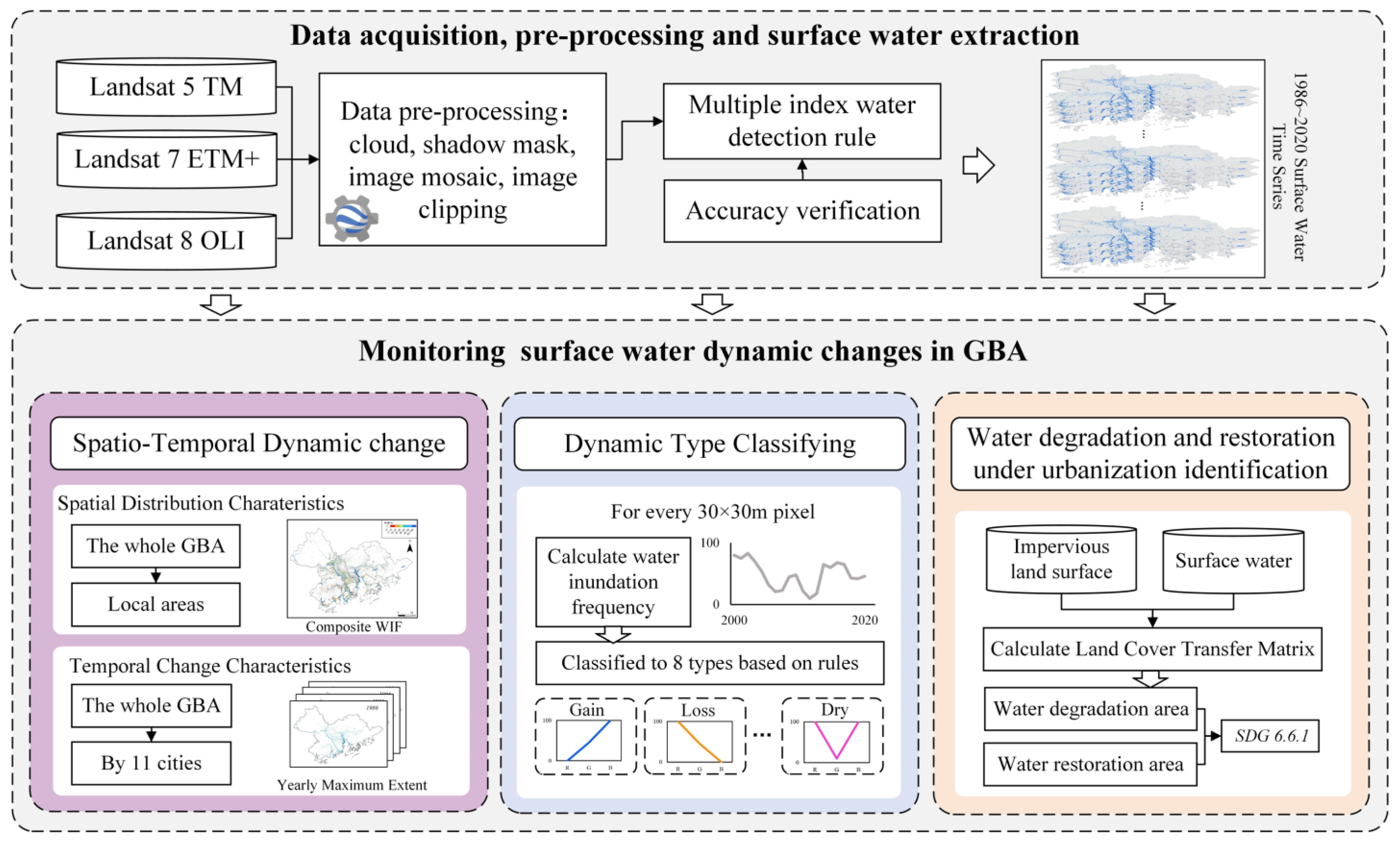
utilizing all available Landsat TM, ETM+ and OLI data from 1986 to 2020 and the GEE platform, to extract long-term surface water extent based on a multi-index water extraction method to explore its spatial variations and temporal change trends (by OLS-RS method) of surface water extent in the GBA;
(2)
to achieve surface water dynamic type classification and mapping based on multiyear water inundation frequency time-series;
(3)
to analyze the impact of urbanization on surface water losses and gains quantitively from the aspect of realizing SDG 6.6.1 and discuss the possible climate causes for water area changes in the GBA.

2. Materials and Methods
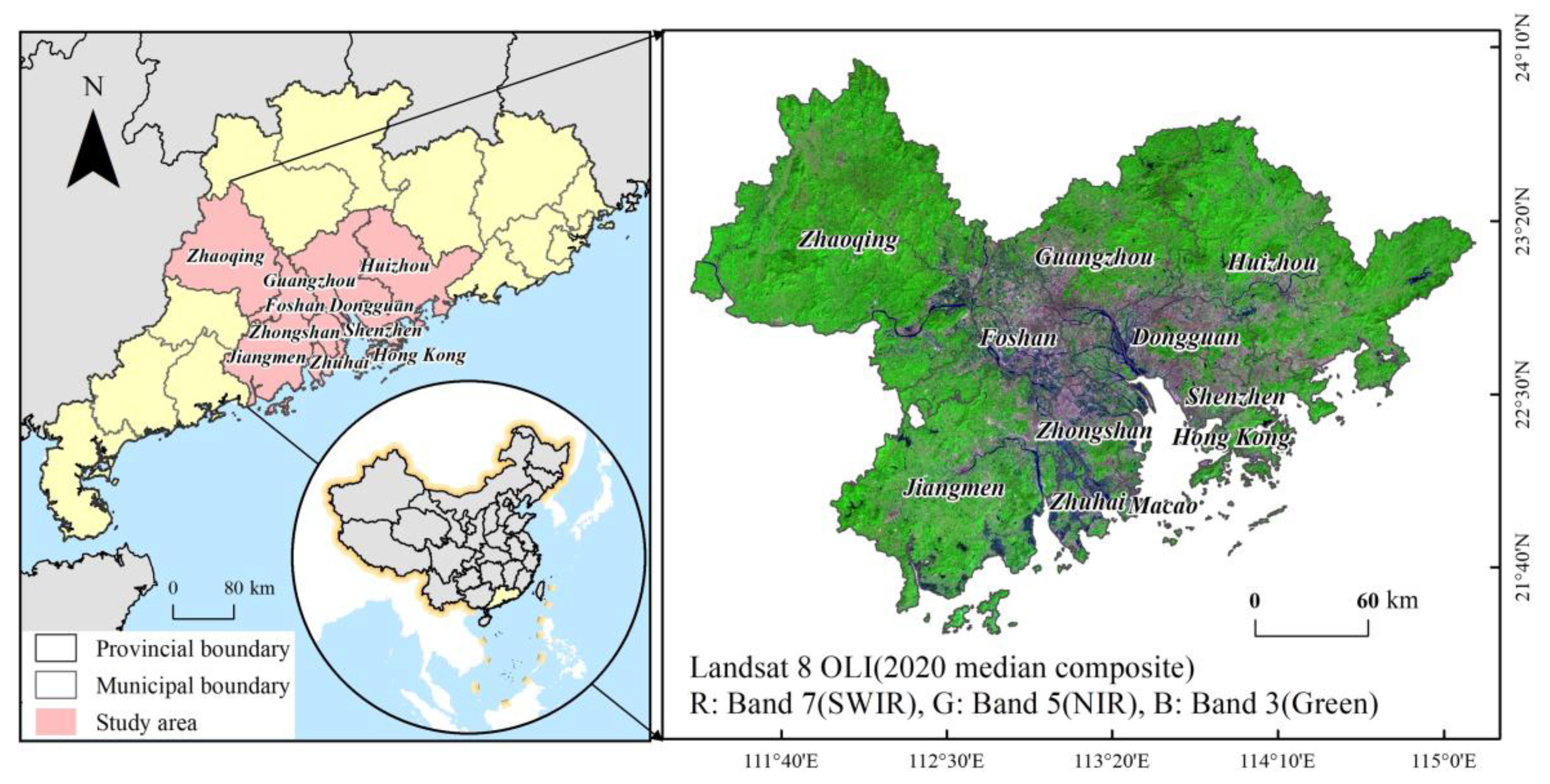
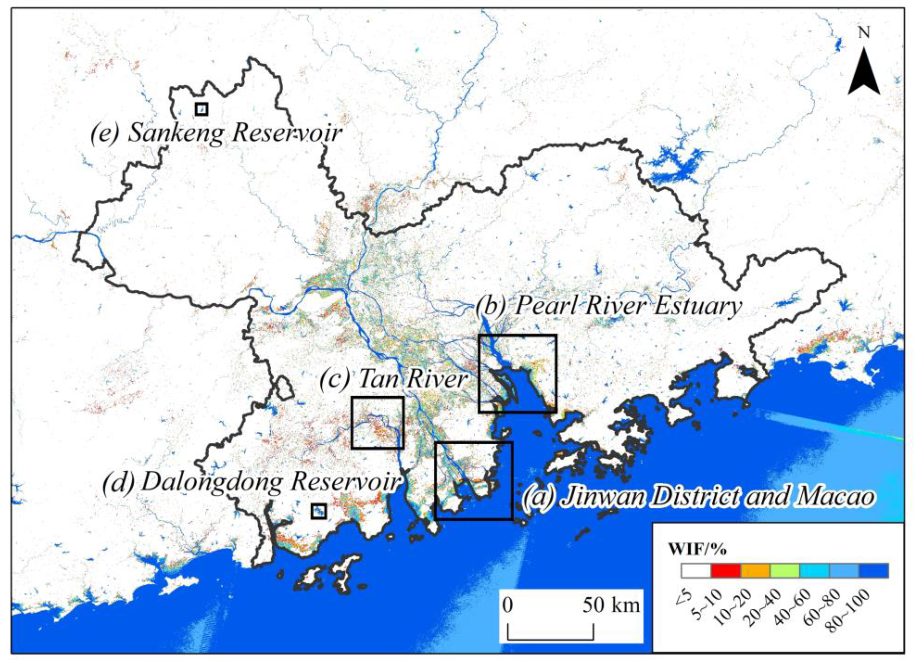
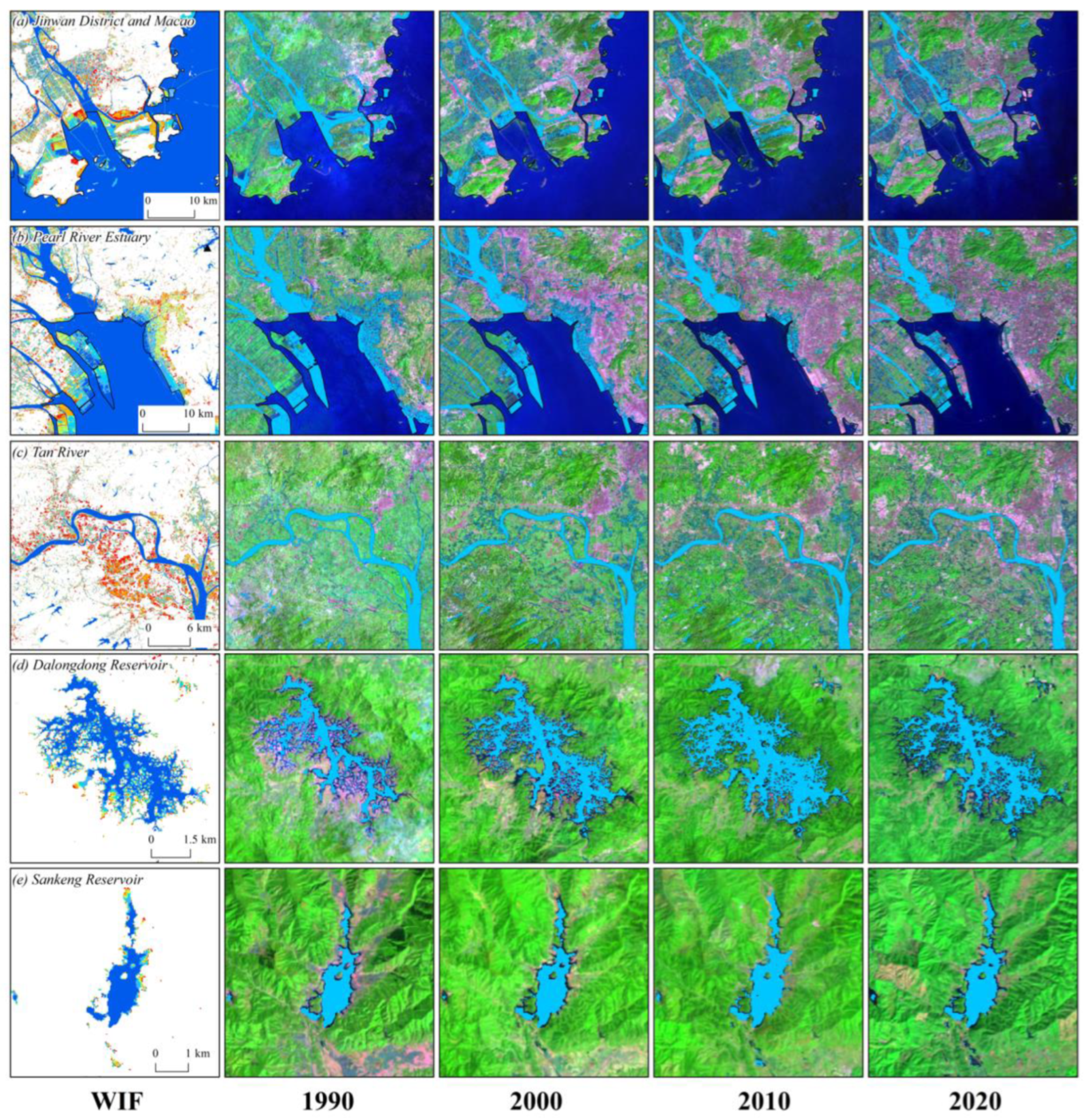
2.1. Study Area

Located in the southern coastal area of China, the GBA (latitude: 111°20′E–115°24′E, longitude: 21°32′N–24°26′N) is a region across nine cities of Guangdong Province and two special administrative regions, which includes Zhaoqing, Guangzhou, Huizhou, Foshan, Dongguan, Jiangmen, Zhongshan, Shenzhen, Hong Kong and Macao, as shown in Figure 1. The total area of the GBA is approximately 56,000 km2. In addition, the GBA is situated in the humid subtropical monsoon climate zone, with abundant rainfall during rainy and hot periods (from April to September); its annual precipitation is approximately 1300~2500 mm, and its annual average temperature is approximately 22 °C [34,35,36].
With a total population of more than 86 million people and regional GDP of approximately USD 1668.8 billion at the end of 2020, which was equivalent to 12% of the GDP for all of mainland China, the GBA is the largest and richest economic region in South China. The GBA is also the starting point of the Maritime Silk Road and the gateway of China to the world [37].

2.2. Datasets and Preprocessing
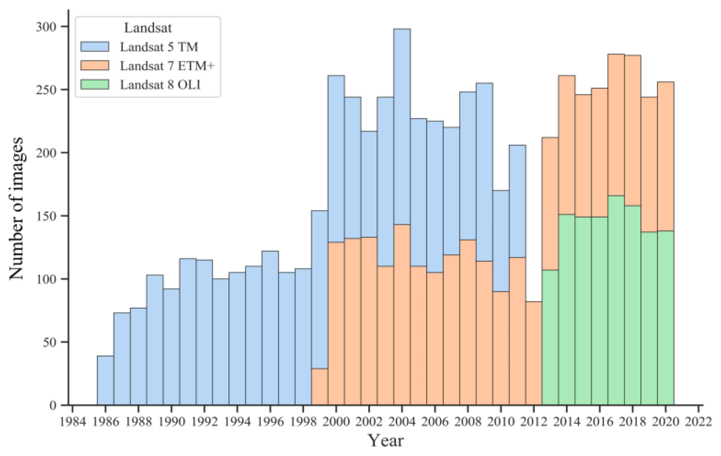
2.2.1. Landsat Data

In this study, we selected Landsat satellite images to extract water areas in the GBA. With a 30-m spatial resolution and 16-day temporal revisit period, all available Landsat 5 TM, 7 ETM+ and 8 OLI surface reflectance images covering the entire GBA from 1986 to 2020 were utilized and processed on the GEE platform for convenience and efficiency. The temporal distribution of image quantities for three remote sensors is shown in Figure 2, which includes scenes with 121/43, 121/44, 122/43, 122/44, 122/45, 123/42, 123/44 and 123/45 as path/row values. The number of images totals 4750, and a rapid decrease in the number of images took place in 1999 due to the launch of Landsat 7. The year 2012 witnessed a dramatic drop in the number of images for Landsat 5 ceased to function, followed by a sharp growth in 2013 caused by the launch of Landsat 8.
In addition, for each image, we removed the cloud, cloud shadow, and snow/ice according to the pixel quality attributes of the Landsat surface reflectance product, which were generated from the Fmask algorithm [38]. The preprocessed Landsat time series was used to extract the surface water extent in the GBA.

2.2.2. Auxiliary Data

The Joint Research Centre of European Commission (JRC) Monthly Water History (v1.2) data (https://esdac.jrc.ec.europa.eu/, accessed on 28 June 2021), created by Pickens et al. [3], were used as ancillary data for comparison with the surface water extent extracted by MIWDR [26] in the GBA.
The impervious land surface data were used in this study to represent the extent of urbanization. The data is from the annual maps of global artificial impervious area (GAIA) between 1985 and 2018 by Gong et al. [39,40] (http://data.ess.tsinghua.edu.cn/gaia.html, accessed on 28 June 2021). In addition, the mean overall accuracy of GAIA over multiple years (1985, 1990, 1995, 2000, 2005, 2010, and 2015) is higher than 90% and the spatial resolution of GAIA is 30 m.
Moreover, annual rainfall data were collected from the Cas Resources and Environment Cloud Platform (https://www.resdc.cn/Default.aspx, accessed on 28 June 2021) to explore the correlation relationship between surface water area and climate change.

2.3. Methodology

For clarity and brevity, we established an analytical framework to systematically and quantitively characterize the long-term dynamics of surface water in the GBA for reporting SDG 6.6.1 indicator (Figure 3). It is divided into two sections: (1) First, we performed data acquisition, preprocessing and surface water extent extraction on the GEE platform to retrieve long time series surface water results for subsequent dynamics analysis. (2) Second, using the surface water datasets obtained above, we analyzed the changes in surface water from three aspects: ① The spatial distribution and temporal characteristics of surface water extent were analyzed in the whole GBA and by 11 cities. ② The annual water inundation frequency time-series for every 30 m×30 m pixel in the GBA was calculated, and dynamic type classification and mapping were carried out based on the temporal variation of the WIF. ③ Combined with impervious land surface data and a land cover transfer matrix, the regions with water losses and gains were identified and analyzed for reporting SDG 6.6.1 indicators.

2.3.1. Water Extraction Based on Multiple Index Water Detection Rule

In this study, we employed a simple and fast automatic water extraction method, the multiple index water detection rule (MIWDR), developed by Deng et al. [26], to retrieve surface water time series during 1986–2020 in the GBA for subsequent analysis. The method utilized multiple indices, including NDVI, EVI, MNDWI, and AWEI. Equations (1)–(5) of these indices are as follows:
NDVI = ρ N I R ρ R e d ρ N I R + ρ R e d
EVI = 2.5 × ρ N I R ρ R e d 1 + ρ N I R + 6 × ρ R e d 7.5 × ρ B l u e
MNDWI = ρ G r e e n ρ S W I R 1 ρ G r e e n + ρ S W I R 1
AWEI n s h = 4 × ( ρ G r e e n ρ S W I R 1 ) ( 0.25 × ρ N I R + 2.75 × ρ S W I R 2 )
AWEI s h = ρ B l u e + 2.5 × ρ G r e e n 1.5 × ( ρ N I R + ρ S W I R 1 ) 0.25 × ρ S W I R 2
where ρ N I R , ρ R e d , ρ B l u e , ρ G r e e n , ρ S W I R 1 and ρ S W I R 2 represent the values of the near infrared band, red band, green band, shortwave infrared band1 and band2 in the Landsat Images.
If a pixel meets the following criteria: (AWEInsh−AWEIsh > −0.1) and (MNDWI > NDVI or MNDWI > EVI), then it is classified as a water body, if not, it is classified as a non-water body. The MIWDR could be implemented quickly through JavaScript codes based on the GEE cloud computing platform. Compared to other relatively complex machine learning methods, this method has the advantages of simplicity, efficiency, high automation, the capacity to quickly acquire the latest surface water information for analysis.
In addition, we assessed the accuracy of surface water results based on MIWDR method by comparing with the actual visual interpretation results from Landsat true color images. The sample points were created randomly (300 random sample points were selected for each imagery in the study) in each Landsat image tile (10 images in total) via the Create Random Points tool in ArcGIS. These sample points were classified into water and non-water types according to visual interpretation, then a confusion matrix was calculated with the extracted surface water results at the same time. The final accuracy assessment result was presented through overall accuracy and kappa coefficient [21].
Furthermore, we also compared the extracted surface water results with the existing water dataset—the Joint Research Centre of European Commission (JRC) Monthly Water History (v1.2) data in the GBA. The relative error (RE) of surface water extent was calculated to measure the accuracy between the two water datasets. The formula to calculate RE is as follows:
R E = ( | S a S e | S e ) × 100 %
where S a respects the surface water area of JRC water dataset, and S e is the surface water area of the extracted water dataset using MIWDR.

2.3.2. Change Trend Analysis Method

Regression analysis is an important method to explore the statistical correlation relationship between different variables and is also suitable for studying the long-term change trend of land surface variables. In this study, the ordinary least square linear regression (OLS-LR) model was used to conduct regression analysis on the time variable x and the surface water area variable y, which could be expressed by the following mathematical formula [41]:
y = a + k x + ε
In the formula, a is a constant; k is the slope of the linear regression equation; x is the time variable, and ε represents the random error value. This study utilized the least square method to fit the linear relationship between a series of surface water areas and time-series values. The parameter k was used to measure the linear change trend of time-series data. When k > 0, it represents an upward trend; otherwise, it denotes a downward trend. Moreover, the value of k represents the change speed of surface water extent per year. The k is calculated as follows:
k = i = 1 n ( x i x ¯ ) ( y i y ¯ ) i = 1 n ( x i x ¯ ) 2
x ¯ = 1 N i = 1 n x i , y ¯ = 1 N i = 1 n y i
In Formulas (2) and (3), x i represents the time value of year i; y i is the surface water area of year i, and N and n represent the total number of observation data points.
Moreover, the goodness of fit test is assessed by using the decisive coefficient R2. The closer R2 is to 1, the closer the whole time-series dataset is to the linear regression line, and the higher the goodness of fit. We applied the OLS-LR over the temporal change analysis in the entire study area as well as 11 cities in the GBA to investigate the surface water extent change trends.

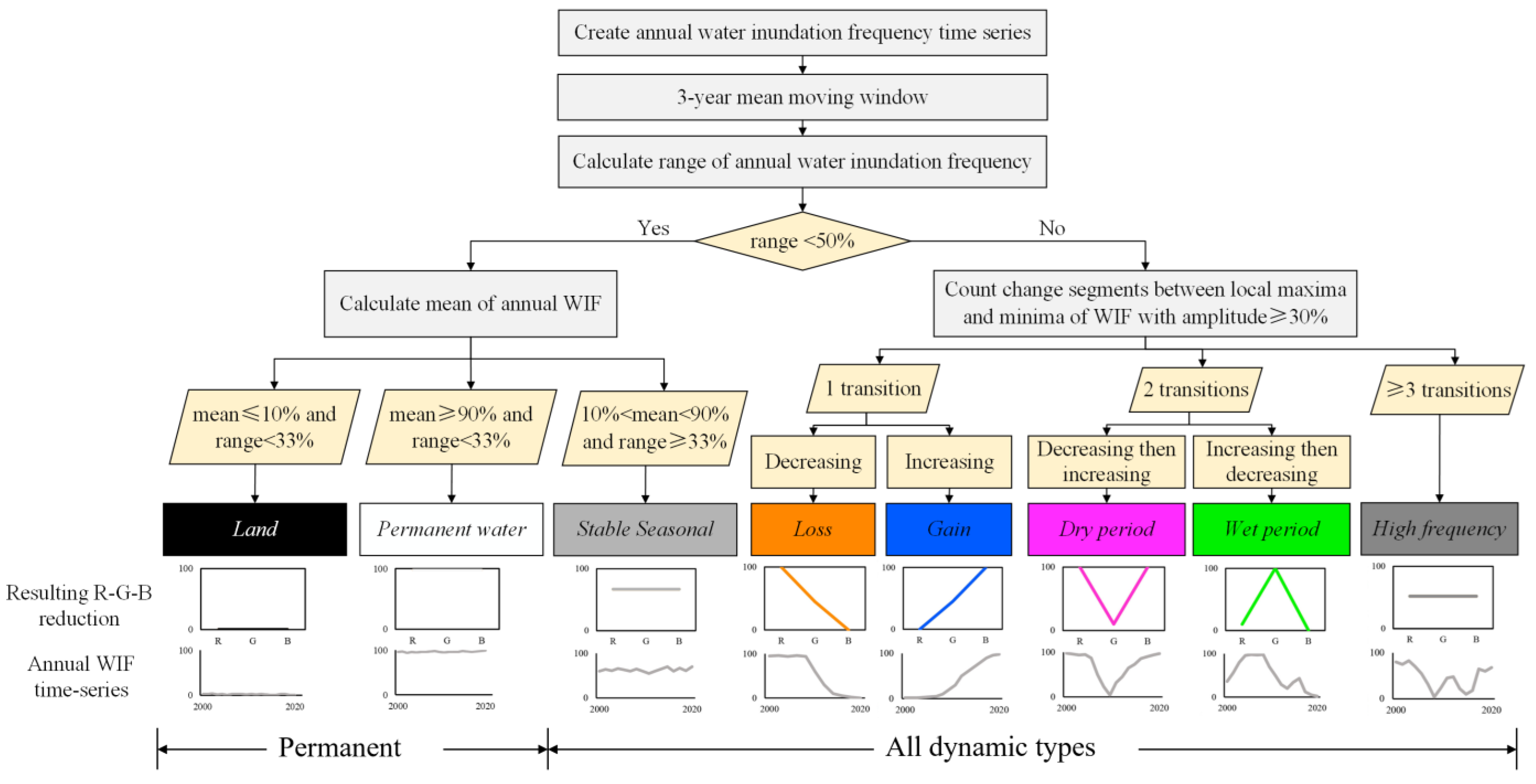
2.3.3. Dynamic Type Classification

Before performing surface water dynamic type classification, we calculated the annual water inundation frequency (WIF) time-series from 2000 to 2020 for each 30 m × 30 m pixel across the study area, considering the Landsat images’ quantity over time (Figure 2). The WIF index directly indicates the frequency of water body occurrence during a certain period of time. The calculation formula of WIF [21] is as follows:
WIF = i = 1 N ( ε i = 1 ) N × 100 %
where ε i represents the corresponding pixel value of the ith water map, where 1 is water and 0 is non-water; i = 1 N ( ε i = 1 ) is the total number of observations of water body occurrence, and N represents the total number of valid observations at a specific pixel.
Based on the annual WIF time-series of the GBA obtained above, the long time-series dynamic types during 2000–2020 were classified pixel-by-pixel using the mean and range. The thresholds’ setting of mean and range was referred to Pickens et al. [42]. The detailed dynamic type classification process for every pixel is shown in Figure 4. Firstly, to reduce annual anomalies, the yearly WIF time-series were smoothed through a three-year average moving window. Secondly, the range and mean of the annual WIF time-series data of each pixel over the period were calculated. The range is the difference between the maximum and minimum value of WIF. In addition, the amount of local extreme values reaching 30% of the range was calculated as the value of WIF change segments. Meanwhile, the permanent and dynamic types of surface water were visualized in RGB color space is visualized according to the WIF change points. The WIF values at the starting position, ending position, and turning position were taken as the values of the red, green and blue channels, respectively. Finally, we achieved surface water dynamic type classification and visualized the spatial distribution.

2.3.4. Identifying Water Losses and Gains under Urbanization

Considering that the GBA is a typical area of rapid urbanization, this study emphasizes the impact of urbanization on the losses and gains of surface water in the study area. Therefore, we only calculated the conversion between surface water bodies and impervious land surfaces through the land cover transition matrix. The land cover transition matrix is the application of the Markov model in land use and land cover, which can quantitatively measure the transformation of different land use types. Furthermore, in order to analyze the spatiotemporal variation in surface water changes by urbanization, we selected seven periods, including 1986, 1990, 1995, 2000, 2005, 2010 and 2015, to calculate the corresponding surface losses and gains under urbanization.

3. Results

3.1. Accuracy of Extracted Surface Water Bodies in the GBA

A total of 10 images with little cloud coverage (less than 5%) and good quality were selected for accuracy evaluation. These images are evenly distributed every 2–3 years from 1993 to 2020 and cover varied months. As seen from Table 1, the RE (relative errors) of the water area extracted in this study and the JRC water products in the same months are small, ranging from 0.5% to 7.5%, with an average of 4.07%. This indicates that the water area extracted in this study is relatively consistent with the results of JRC products.
In addition, the overall accuracy and kappa coefficient results of these 10 images are shown in Table 2. The overall accuracy ranged from 89.95% to 96.89%, with an average value of 93.42%, while the kappa coefficient varied between 0.75 and 0.83, with an average value of 0.794, which indicates the accuracy of the surface water extraction results in this study is relatively high.

3.2. Spatial Changes in Surface Water in the GBA from 1986 to 2020 for SDG 6.6.1 Monitoring

The spatial distribution of the WIF in the GBA during 1986–2020 is shown in Figure 5, it was divided it into 6 levels: 5–10%, 10–20%, 20–40%, 40–60%, 60–80% and 80–100%. The higher the WIF value is, the more likely the pixel is to be a permanent water body. The areas of surface water bodies is 1140.62 km2, 1179.98.71 km2, 1253.96 km2, 951.45 km2, 823.59 km2 and 1889.42 km2 under six levels of WIFs mentioned above, and accounts for 19.11%, 15.65%, 16,63%, 12.62%, 10.92% and 25.06% of total water area, respectively. It is also evident that surface water bodies are mainly distributed around the Pearl River Delta and other river networks in the GBA.
When zooming in some typical regions (a, b, c, d and e), it could be seen that the high-WIF area (>80%) tends to be distributed in the center of rivers and lakes, and the WIF in the marginal region of rivers and lakes shows a decreasing trend from inside to outside (Figure 6e). The spatial distribution characteristics are consistent with the natural and hydrological principles of river and lake dynamics, and it is well known that the impact of human activities on water bodies often occurs around surface water Figure 6a,b). In addition, it should be noted that in the interlaced area of river networks, a substantial number of water bodies are distributed in blocks or fragments (Figure 6c), and their WIF values are mostly less than 50%, which could be attributed to the abundance of paddy fields and pits in the region.

3.3. Temporal Changes in Surface Water in the GBA from 1986 to 2020

For the whole GBA, the annual surface water body area calculated under different WIF thresholds from 1986 to 2020 is shown in Figure 7. The permanent surface water bodies (WIF > 75%) did not change much. In contrast, the maximum surface water extent (WIF > 0%) in the GBA demonstrates a significant decreasing tendency after 2001 (R2 = 0.8566, p < 0.0001), with a loss of 155.41 km2 per year. Furthermore, the seasonal surface water extent (35% < WIF < 75%) fluctuates slightly over the last 35 years. It also could be seen that the lower the WIF threshold is, the higher the loss rate after 2001.
The yearly surface body areas of eleven individual cities in the GBA during 1986–2020 showed divergent trends over time (Figure 8). For better separation, we classified these cities into three groups to illustrate their change characteristics according to the range of surface water area. Furthermore, the linear trend lines were added to the line charts corresponding to each city. Among the cities, the surface water areas in Guangzhou, Foshan, Huizhou, Zhuhai, Shenzhen, Hong Kong and Macao show an evident downward trend. Especially for Macao, the linear declining trend in Macao is very significant, with R2 of 0.96, but its loss rate is fairly low, with about 0.426 km2 per year. It is noteworthy that there are no cities with a significant upward trend here, which reflects that the majority of cities are experiencing a decrease in surface water areas to varying degrees. Therefore, for cities with a rapid downward trend, more attention should be given to surface water protection and recovery.

3.4. Dynamic Type Mapping and Analysis in the GBA during 2000–2020

The dynamic type map for surface water variations during 2000–2020 in the GBA is illustrated in Figure 9, in which the color represents varied dynamic types (seen in Figure 4). As seen in some typical enlarged areas of dynamic types, the edge of the lake in subregion A is orange, and the central area of the lake is white, which indicates the surface water around the lake is losing. In contrast, the blue edge of the lake in subregion B presents an expansion trend. Some patches experiencing a dry period (with WIF growing down first and up later) in paddy fields in the subregion C are pink, while the green region of the meandering river streamway (in the subregion D) denotes that it witnessed a wet period in history. The lakes with light gray edges in subregion E experience seasonally stable changes, which could be attributed to the regular hydrological phenology. The paddy fields in subregion F exhibit signs of high-frequency changes, which may be caused by intensive human activities.
The statistics of dynamic type classification results are presented in Table A1 in detail and visualized in Figure 10. All water-related areas account for 6.48% (3594.01 km2) of the total area in the GBA, of which 57.46% was dynamic types during 2000–2020. This suggests that most surface water bodies change over the last 20 years instead of remaining unchanged. In addition, the gain, loss, dry and wet periods account for approximately 4–7% of all areas with water, while stable seasonal and high-frequency periods account for approximately 16–18% of all areas with water. The difference in areas indicates that the surface water area experiencing multi-direction changes is greater than that of single-direction changes. In reality, to support the achievement of SDG 6.6.1, areas of loss should be given more attention from local governments and residents.

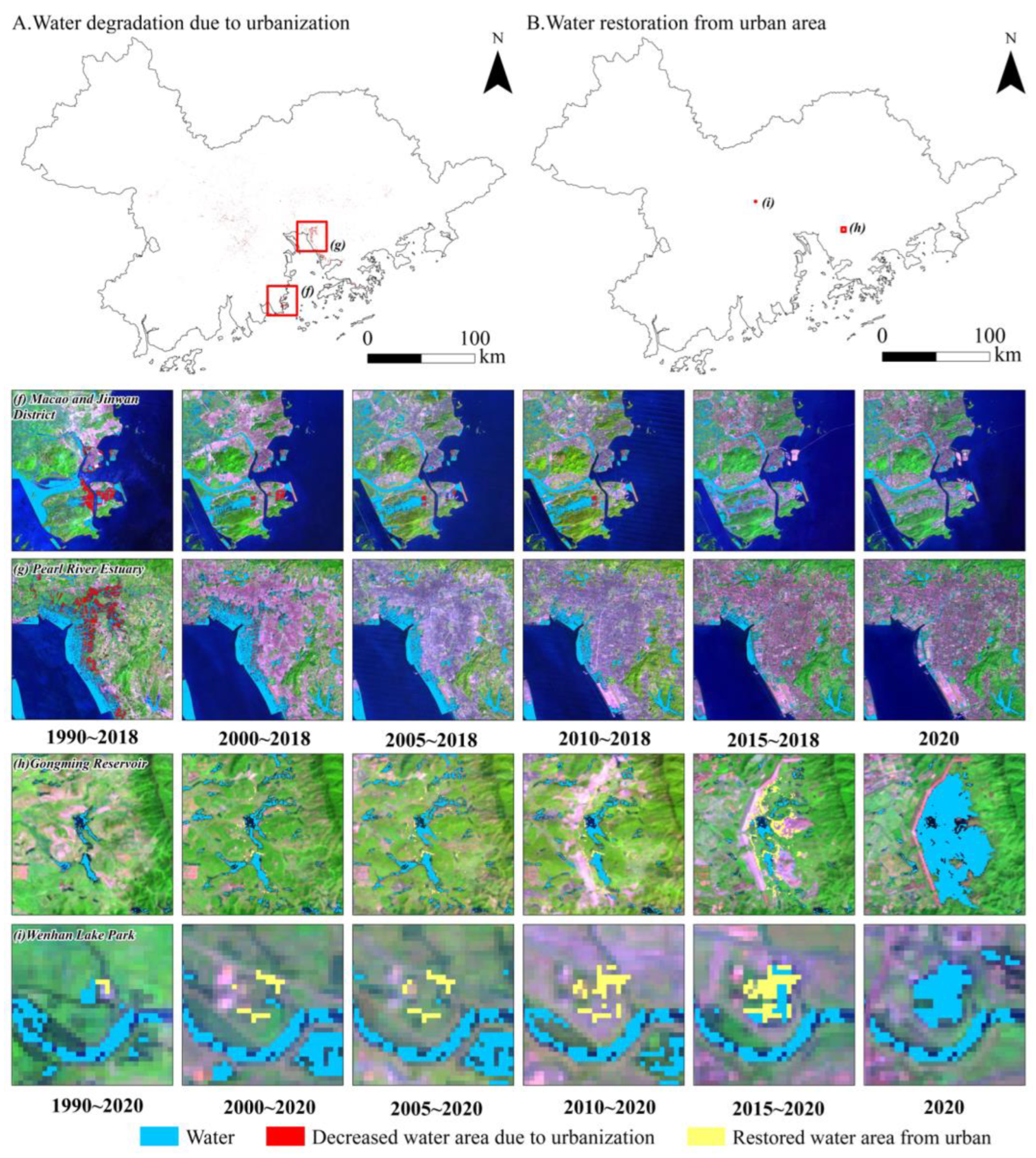
3.5. Surface Water Losses and Gains under Urbanization in the GBA

The overall spatial distribution of surface water losses and gains is shown in Figure 11A,B. In the two enlarged regions (Figure 11f,g) of water losses, it was found that many cities and towns occupy water bodies in coastal areas and the reclamation of coastal urban zones. In the zoomed region (Figure 11h,i) of water gains, some built-up areas are transformed into water due to the construction of artificial reservoirs and lake parks, like Gongming reservoir and Wenhan Lake Park. In general, the area of water bodies occupied by urbanization is far greater than that restored to water bodies.
Through the land cover confusion transfer matrix, the area of water bodies transformed into impervious surfaces and the area of built-up areas transformed into water bodies in different years were calculated(Figure 12). The surface water losses area shows a significant declining trend from 211.29 km2 in 1986 to 2.92 km2 in 2015 (Figure 12a), and the surface water restoration area shows a slightly growing trend (Figure 12b), which indicates that more water bodies have been protected in recent years and that more attention has been given to water restoration.

4. Discussion

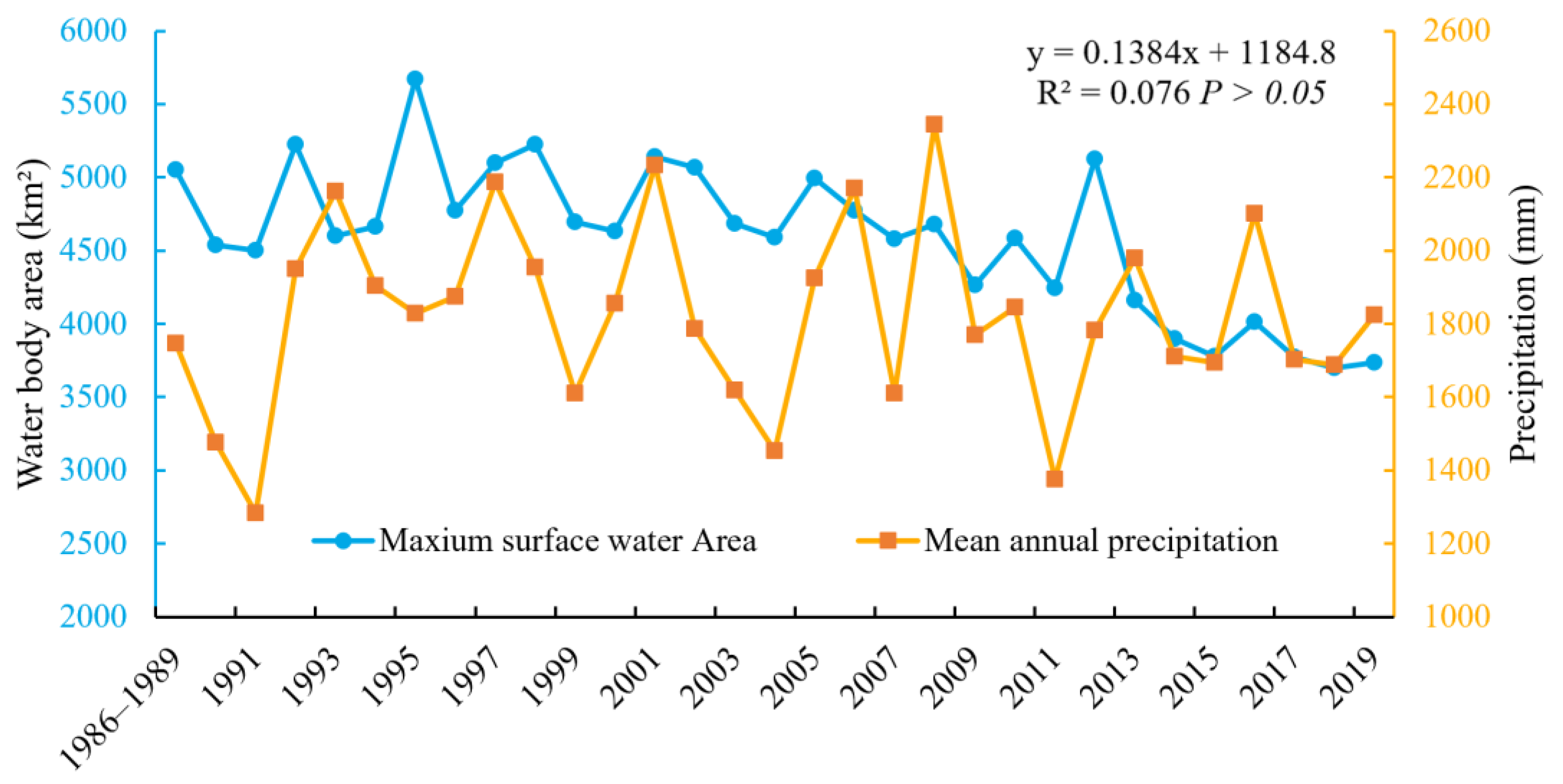
4.1. Possible Causes for Surface Water Extent Changes

Climate change is an important factor that may affect surface water area. Precipitation is a key component of climatic factors, which has a complicated relationship with surface water extent changes. We briefly analyzed the relationship between precipitation and maximum surface water extent by comparing the changes during 1986–2019. We also calculated the linear correlation coefficient between them (Figure 13). The change trend of precipitation and surface water extent was inconsistent and the linear correlation between them is not significant (p < 0.05), but the change trend was relatively consistent over some short-term periods, which may be caused by extreme precipitation events.

4.2. Comparison with Other Studies

Comparing the surface water area derived in this study with the result of other researchers, it is found that the results are highly consistent. According to the study of Zhao Y L, et al. [43], the surface water area of the GBA in 2015 was 5266.02 km2, which was obtained based on remote sensing data used in the Second National Land Survey, China, in 2015 and checked for correctness. While the maximum surface water area of the GBA in 2015 was 5318.80 km2 in this study, the difference between the two results was 52.78 km2, which further verified the reliability of the surface water results in this study. However, we are not able to compare the temporal variations due to a lack of relevant studies in the GBA.
In addition, the surface water monitoring and analysis method and framework of this study features by efficiency of the GEE platform and serving the goal of SDG 6.6.1. The most important point is that we analyzed the dynamic types of surface water to characterize and visualize the spatiotemporal variations for reporting SDG 6.6.1 in the study area. In comparison with previous studies related to surface water extraction and SDG 6.6.1 [2,21], this study’s analytical framework is more refined and comprehensive.

4.3. Implications for SDG 6.6.1 Reporting and Policy-Making

Since the SDG 6.6.1 indicator aims to track variations in different types of water-related ecosystems, informing decision-makers of the extent changes of water-related ecosystems over time, the workflow, framework and analysis of this study are highly consistent with these targets, which might be taken as references for other similar studies related to SDG 6.6.1 reporting and policy-making of regional government for sustainable development.
Additionally, from the surface water extent spatiotemporal variations derived in this study, it is evident that the surface water area in the GBA shows a slow downward trend in recent 35 years and the surface water area keeping losing occupies 7.34% (263.75 km2) of all water-related area in the GBA. Therefore, more attention should be paid to regions experiencing decreasing trends to pre-empt further loss in surface water resources.

4.4. Limitations and Future Improvements

There are still some limitations and uncertainties in this study.
(1)
The Landsat imagery used in this study is easily affected by clouds, and the GBA is a typical coastal region with frequent cloud coverage. This issue limits the highly frequent monitoring of surface water when it comes to extreme disasters (e.g., extreme precipitation events) in the GBA.
(2)
In regard to surface water verification, we selected ten images for accuracy assessment, the number of images is relatively small and the evaluation of images with a medium or high cloud coverage was not taken into consideration, which could cause some uncertainties to the surface water results.
(3)
The exploration of driving factors of long-term surface water variations is still not enough. We only analyzed the impact of land cover change and precipitation on the surface water changes. Due to low accessibility to more meteorological and hydrological in the GBA and the complexity of mutual influence mechanism between human activities and climate changes, we did not use more datasets to make a comprehensive analysis of the driving forces.
In the future research, we will optimize the data preprocessing procedures to reduce the effects of clouds on the optical remote sensing imagery and introduce other multi-source remote sensing data, such as Sentinel 1/2, HJ, GF and other data with high resolution and quality to better monitor the spatiotemporal dynamics of surface water in the study area. Additionally, we need to apply multi-factor analysis to investigate the driving forces of surface water changes in the GBA more comprehensively. Moreover, we are supposed to integrate.

5. Conclusions

In this study, in order to monitor SDG 6.6.1 indicator, we utilized long-term Landsat images and the MIWDR method to extract surface water extent of the GBA during 1986–2020 on the GEE platform. We characterized the spatial and temporal variations in surface water in the GBA and classified dynamic types of surface water by pixels to explore the features of surface water dynamics in detail. In addition, the surface water losses and gains caused by urbanization were identified and analyzed. The main conclusions are as follows:
(1)
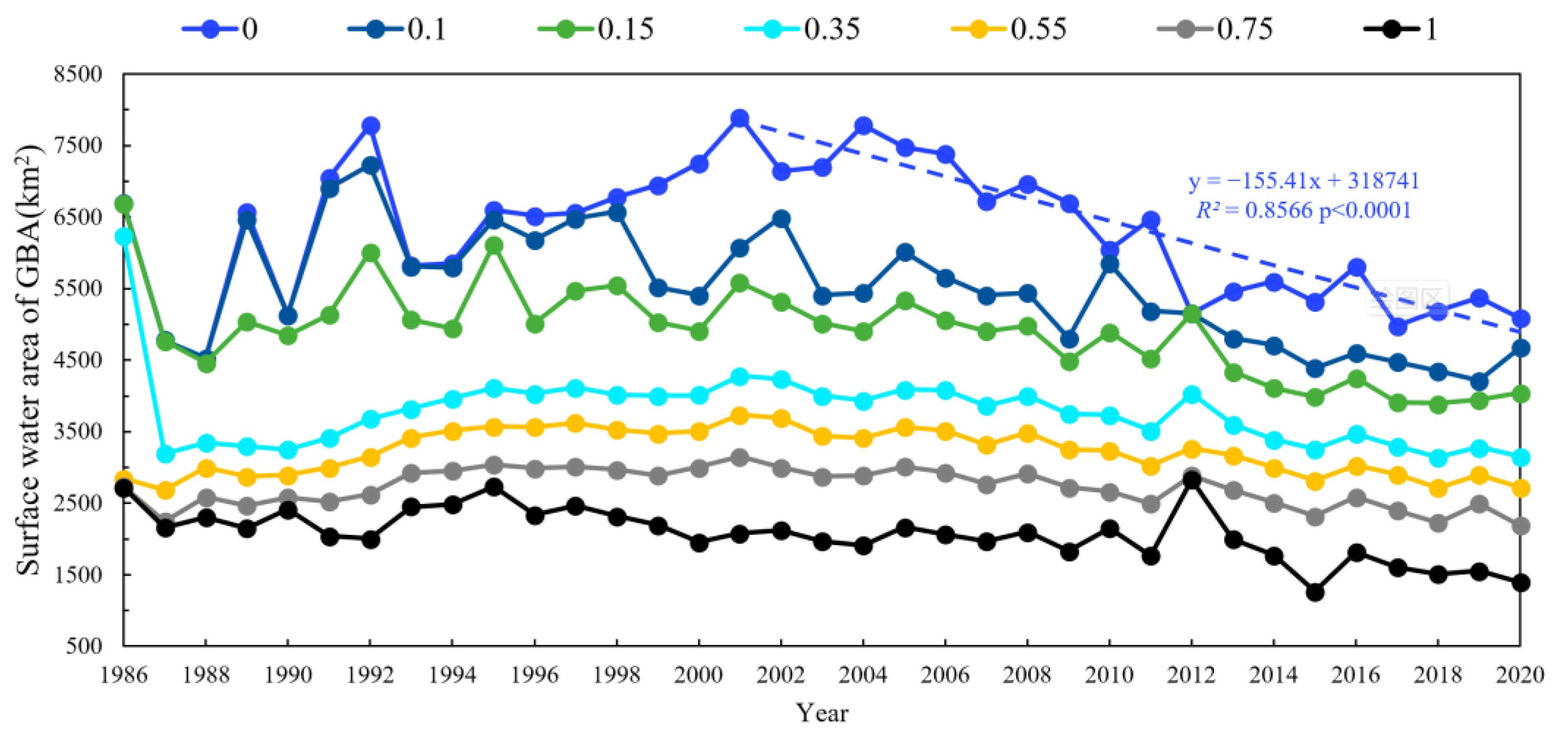
From 1986 to 2020, the average minimal and maximal surface water extents of the GBA were 2017.62 km2 and 6129.55 km2, respectively. The maximum areas fell rapidly from 7897.96 km2 to 5087.46 km2, with a loss of 155.41 km2 per year, which showed a significant downward trend. The surface water extents calculated by water inundation frequency thresholds greater than 0.35 fluctuate slightly during this period. This denotes that permanent and part of seasonal surface water in the GBA stay relatively stable in the last 35 years. It is noticeable that there exists a slow downward trend in surface water area after 2001.
(2)
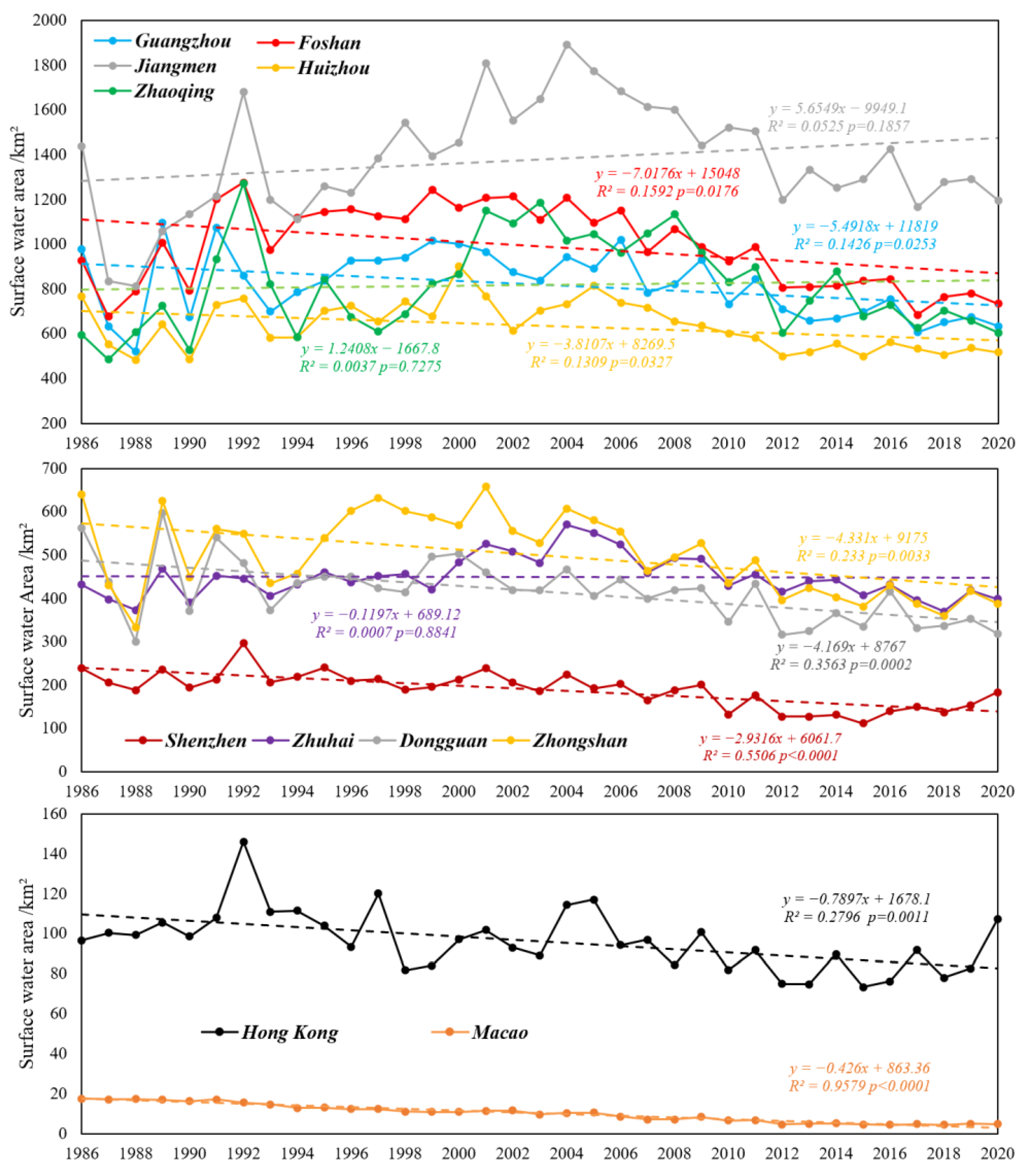
The surface water extent in most cities demonstrates a downward trend with varying loss speed. Especially for Foshan, Guangzhou, Zhongshan and Huizhou, the decreasing trend is evident compared with other cities in the GBA. More attention from local government should be given to cities with intense declining trends.
(3)
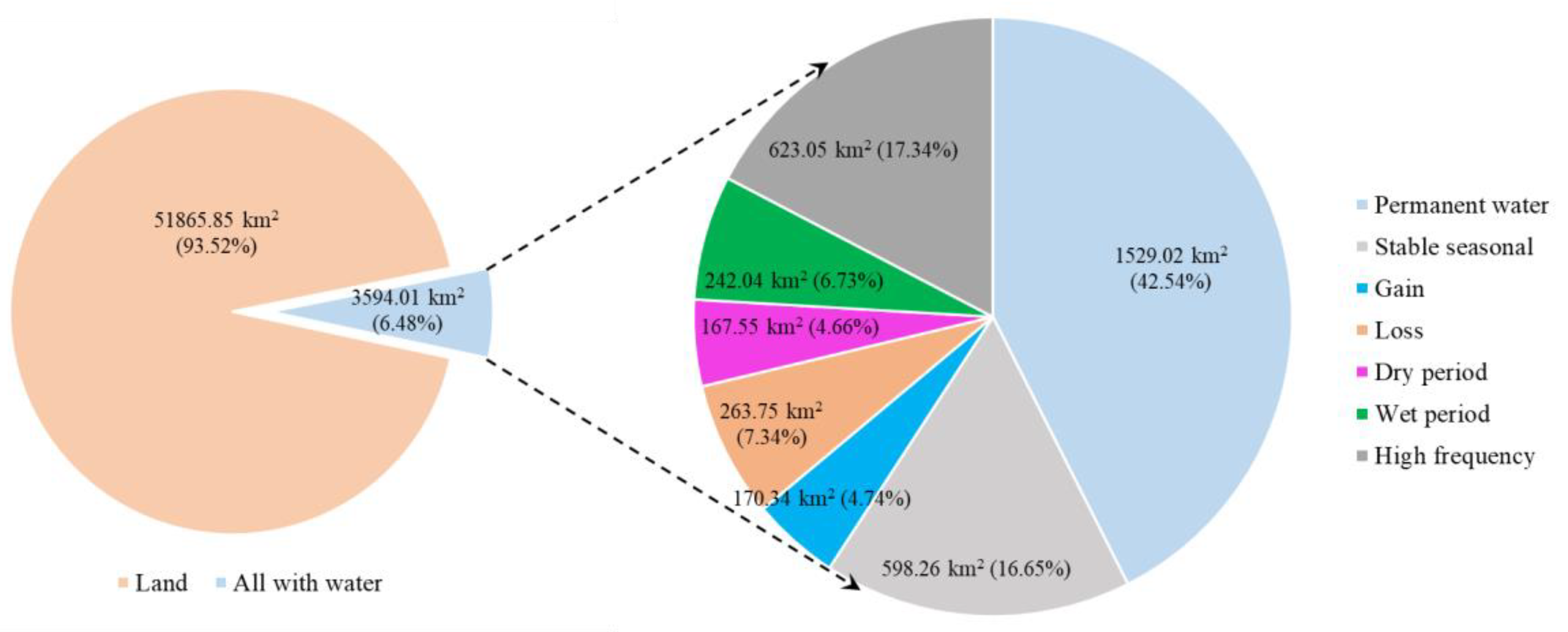
The areas of permanent water bodies and dynamic water bodies were 1529.02 km2 and 2064.99 km2, accounting for 42.54% and 57.46% of the total water area, respectively. The statistics reflect that most surface waters are in a changing state.
(4)
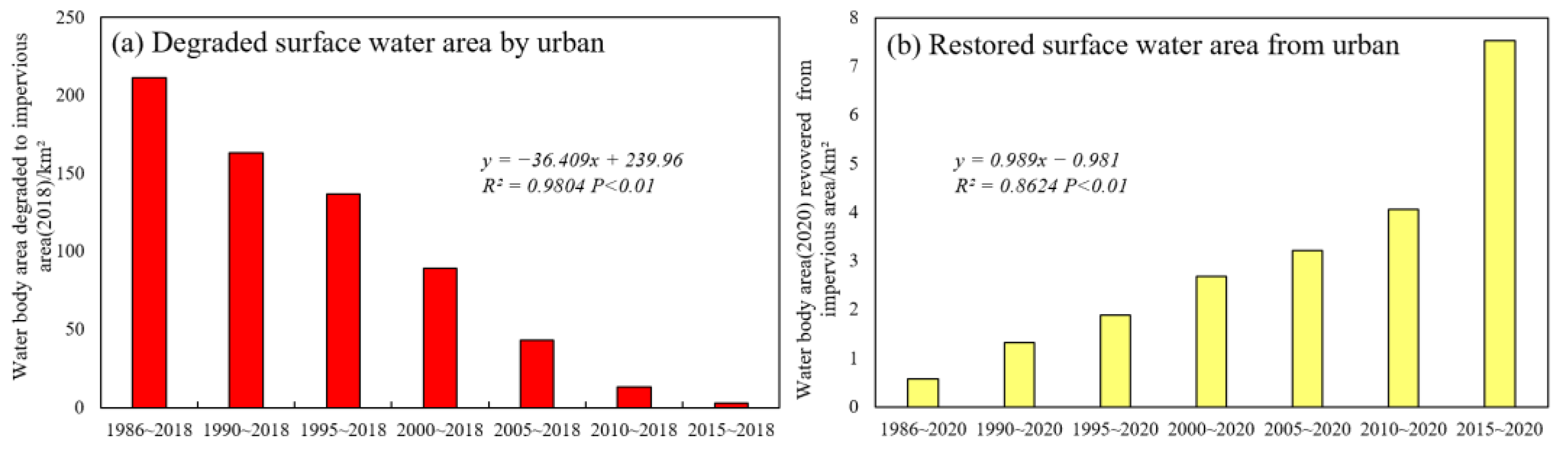
The surface body area occupied by impervious land surfaces showed a significant linear downward trend with R2 values of 0.98 and 36.41 km2 per year, while the surface water restored from impervious land surfaces denoted a slightly growing trend. It appears that surface water extent is under less pressure induced by urbanization in recent years and has more chances to be restored and protected by human activities.
In addition, we also assessed the water extraction accuracy and possible climate factors for surface water changes. However, due to the uncertainties and limitations that existed in our study, we need to further explore other factors affecting the surface water extent of GBA in following research.
In this study, the long-term surface water time-series datasets and spatiotemporal analysis results could be provided for reference by local governments or related ecological environment protection agencies to assess regional procedures toward achieving SDG 6.6.1 as well as to inform environmental protection policy-makers of the key areas for water conservation and restoration in the GBA. Furthermore, the methodology, analytical framework and remote sensing big data resources available on the GEE could be easily applied in other similar regions worldwide for supporting the SDG 6.6.1 indicator and promoting regional water resources protection as well as management.

Author Contributions

Conceptualization, W.J., Z.W. and Z.L.; methodology, Y.D. (Yue Deng) and Y.D. (Yawen Deng); software, Y.D. (Yawen Deng); validation, Y.D. (Yawen Deng) and K.P.; formal analysis, K.P.; investigation, Y.D. (Yawen Deng); resources, W.J. and Z.W.; writing—original draft preparation, Y.D. (Yawen Deng); writing—review and editing, Y.D. (Yawen Deng)., K.P.; visualization, Y.D. (Yawen Deng); funding acquisition, W.J., Z.W. and Z.L. All authors have read and agreed to the published version of the manuscript.

Funding

The research was funded by the NSFC-Guangdong Joint Foundation Key Project, China (Project No. U1901219), the National Natural Science Foundation of China (Project No. 42071393, Project No. 42101369) and the Youth Teacher Scientific Research Ability Improvement Project of Guangxi (Grant No. 2021KY0393).

Institutional Review Board Statement

Not applicable.

Informed Consent Statement

Not applicable.

Data Availability Statement

Not Applicable.

Acknowledgments

We want to express our respect and gratitude to Chunlin Wang, Xiaoya Wang, Zhuo Li, Yuhao Pan and Xinhao Pan for their help. We also would like to thank the reviewers for their valuable comments and suggestions.

Conflicts of Interest

The authors declare no conflict of interest.

Appendix A

Table A1. The statistics of surface water area for different dynamic types in the GBA.
Area km2Percent of Total AreaPercent of All WaterClass Definition
Land51865.8593.52/Mean WIF ≤ 10% and inter-annual variability ≤ 33%
Permanent water1529.022.7642.54Mean water percent ≥ 90% and inter-annual variability ≤ 33%
Stable seasonal598.261.0816.65Intra-annual variability with inter-annual variability < 50%
Gain170.340.314.74Land-dominant to water-dominant
Loss263.750.487.34Water-dominant to land-dominant
Dry period167.550.304.66Water-dominant to land-dominant to water-dominant
Wet period242.040.446.73Land-dominant to water-dominant to land-dominant
High frequency623.051.1217.343+ transitions between water-dominant and land-dominant
Multiple transitions1032.641.8628.73Dry period, wet period, and high frequency (2+ transitions)
All change types1466.732.6440.81Gain, loss, dry period, wet period, high frequency
All dynamic types2064.993.7257.46Gain, loss, dry period, wet period, high frequency, stable seasonal
All with water3594.016.48100Permanent water, stable seasonal, gain, loss, dry period, wet period, high frequency

References

  1. Zou, Z.; Xiao, X.; Dong, J.; Qin, Y.; Doughty, R.B.; Menarguez, M.A.; Zhang, G.; Wang, J. Divergent trends of open-surface water body area in the contiguous United States from 1984 to 2016. Proc. Natl. Acad. Sci. USA 2018, 115, 3810–3815. [Google Scholar] [CrossRef] [Green Version]
  2. Jiang, Z.; Jiang, W.; Ling, Z.; Wang, X.; Peng, K.; Wang, C. Surface Water Extraction and Dynamic Analysis of Baiyangdian Lake Based on the Google Earth Engine Platform Using Sentinel-1 for Reporting SDG 6.6.1 Indicators. Water 2021, 13, 138. [Google Scholar] [CrossRef]
  3. Pekel, J.; Cottam, A.; Gorelick, N.; Belward, A.S. High-resolution mapping of global surface water and its long-term changes. Nature 2016, 540, 418–422. [Google Scholar] [CrossRef] [PubMed]
  4. UN Water. Progress on Water-Related Ecosystems: Piloting the Monitoring Methodology and Initial Findings for SDG Indicator 6.6.1; UN Water: Geneva, Switzerland, 2018; pp. 807–3712. [Google Scholar]
  5. Anderson, K.; Ryan, B.; Sonntag, W.; Kavvada, A.; Friedl, L. Earth observation in service of the 2030 Agenda for Sustainable Development. Geo-Spat. Inf. Sci. 2017, 20, 77–96. [Google Scholar] [CrossRef]
  6. Fitoka, E.; Tompoulidou, M.; Hatziiordanou, L.; Apostolakis, A.; Höfer, R.; Weise, K.; Ververis, C. Water-related ecosystems’ mapping and assessment based on remote sensing techniques and geospatial analysis: The SWOS national service case of the Greek Ramsar sites and their catchments. Remote Sens. Environ. 2020, 245, 111795. [Google Scholar] [CrossRef]
  7. Weise, K.; Höfer, R.; Franke, J.; Guelmami, A.; Simonson, W.; Muro, J.; O’Connor, B.; Strauch, A.; Flink, S.; Eberle, J.; et al. Wetland extent tools for SDG 6.6.1 reporting from the Satellite-based Wetland Observation Service (SWOS). Remote Sens. Environ. 2020, 247, 111892. [Google Scholar] [CrossRef]
  8. Mueller, N.; Lewis, A.; Roberts, D.; Ring, S.; Melrose, R.; Sixsmith, J.; Lymburner, L.; McIntyre, A.; Tan, P.; Curnow, S.; et al. Water observations from space: Mapping surface water from 25years of Landsat imagery across Australia. Remote Sens. Environ. 2016, 174, 341–352. [Google Scholar] [CrossRef] [Green Version]
  9. Sheng, Y.; Song, C.; Wang, J.; Lyons, E.A.; Knox, B.R.; Cox, J.S.; Gao, F. Representative lake water extent mapping at continental scales using multi-temporal Landsat-8 imagery. Remote Sens. Environ. 2016, 185, 129–141. [Google Scholar] [CrossRef] [Green Version]
  10. Rao, P.; Jiang, W.; Hou, Y.; Chen, Z.; Jia, K. Dynamic Change Analysis of Surface Water in the Yangtze River Basin Based on MODIS Products. Remote Sens. 2018, 10, 1025. [Google Scholar] [CrossRef] [Green Version]
  11. Yang, X.; Qin, Q.; Yésou, H.; Ledauphin, T.; Koehl, M.; Grussenmeyer, P.; Zhu, Z. Monthly estimation of the surface water extent in France at a 10-m resolution using Sentinel-2 data. Remote Sens. Environ. 2020, 244, 111803. [Google Scholar] [CrossRef]
  12. Peng, K.; Jiang, W.; Deng, Y.; Liu, Y.; Wu, Z.; Chen, Z. Simulating wetland changes under different scenarios based on integrating the random forest and CLUE-S models: A case study of Wuhan Urban Agglomeration. Ecol. Indic. 2020, 117, 106671. [Google Scholar] [CrossRef]
  13. Khandelwal, A.; Karpatne, A.; Marlier, M.E.; Kim, J.; Lettenmaier, D.P.; Kumar, V. An approach for global monitoring of surface water extent variations in reservoirs using MODIS data. Remote Sens. Environ. 2017, 202, 113–228. [Google Scholar] [CrossRef]
  14. Klein, I.; Gessner, U.; Dietz, A.J.; Kuenzer, C. Global WaterPack—A 250m resolution dataset revealing the daily dynamics of global inland water bodies. Remote Sens. Environ. 2017, 198, 345–362. [Google Scholar] [CrossRef]
  15. Tulbure, M.G.; Broich, M.; Stehman, S.V.; Kommareddy, A. Surface water extent dynamics from three decades of seasonally continuous Landsat time series at subcontinental scale in a semi-arid region. Remote Sens. Environ. 2016, 178, 142–157. [Google Scholar] [CrossRef]
  16. Yao, F.; Wang, J.; Wang, C.; Crétaux, J. Constructing long-term high-frequency time series of global lake and reservoir areas using Landsat imagery. Remote Sens. Environ. 2019, 232, 111210. [Google Scholar] [CrossRef]
  17. Gorelick, N.; Hancher, M.; Dixon, M.; Ilyushchenko, S.; Thau, D.; Moore, R. Google Earth Engine: Planetary-scale geospatial analysis for everyone. Remote Sens. Environ. 2017, 202, 18–27. [Google Scholar] [CrossRef]
  18. Tang, Z.; Li, Y.; Gu, Y.; Jiang, W.; Xue, Y.; Hu, Q.; LaGrange, T.; Bishop, A.; Drahota, J.; Li, R. Assessing Nebraska playa wetland inundation status during 1985–2015 using Landsat data and Google Earth Engine. Environ. Monit. Assess. 2016, 188, 654. [Google Scholar] [CrossRef] [PubMed]
  19. Wang, C.; Jia, M.; Chen, N.; Wang, W. Long-Term Surface Water Dynamics Analysis Based on Landsat Imagery and the Google Earth Engine Platform: A Case Study in the Middle Yangtze River Basin. Remote Sens. 2018, 10, 1635. [Google Scholar] [CrossRef] [Green Version]
  20. Wang, Y.; Ma, J.; Xiao, X.; Wang, X.; Dai, S.; Zhao, B. Long-Term Dynamic of Poyang Lake Surface Water: A Mapping Work Based on the Google Earth Engine Cloud Platform. Remote Sens. 2019, 11, 313. [Google Scholar] [CrossRef] [Green Version]
  21. Wang, C.; Jiang, W.; Deng, Y.; Ling, Z.; Deng, Y. Long time series water extent analysis for SDG 6.6.1 based on the GEE platform: A case study of Dongting Lake. IEEE J. Sel. Top. Appl. Earth Obs. Remote Sens. 2022, 15, 490–503. [Google Scholar] [CrossRef]
  22. Zhou, Y.; Dong, J.; Xiao, X.; Liu, R.; Zou, Z.; Zhao, G.; Ge, Q. Continuous monitoring of lake dynamics on the Mongolian Plateau using all available Landsat imagery and Google Earth Engine. Sci. Total Environ. 2019, 689, 366–380. [Google Scholar] [CrossRef]
  23. Li, J.; Wang, J.; Yang, L.; Ye, H. Spatiotemporal change analysis of long time series inland water in Sri Lanka based on remote sensing cloud computing. Sci. Rep. 2022, 12, 766. [Google Scholar] [CrossRef]
  24. Jia, K.; Jiang, W.; Li, J.; Tang, Z. Spectral matching based on discrete particle swarm optimization: A new method for terrestrial water body extraction using multi-temporal Landsat 8 images. Remote Sens. Environ. 2018, 209, 1–18. [Google Scholar] [CrossRef]
  25. Wang, X.; Wang, W.; Jiang, W.; Jia, K.; Rao, P.; Lv, J. Analysis of the Dynamic Changes of the Baiyangdian Lake Surface Based on a Complex Water Extraction Method. Water 2018, 10, 1616. [Google Scholar] [CrossRef] [Green Version]
  26. Deng, Y.; Jiang, W.; Tang, Z.; Ling, Z.; Wu, Z. Long-Term Changes of Open-Surface Water Bodies in the Yangtze River Basin Based on the Google Earth Engine Cloud Platform. Remote Sens. 2019, 11, 2213. [Google Scholar] [CrossRef] [Green Version]
  27. Wang, X.; Xie, S.; Zhang, X.; Chen, C.; Guo, H.; Du, J.; Duan, Z. A robust Multi-Band Water Index (MBWI) for automated extraction of surface water from Landsat 8 OLI imagery. Int. J. Appl. Earth Obs. 2018, 68, 73–91. [Google Scholar] [CrossRef]
  28. Han, Q.; Niu, Z. Construction of the Long-Term Global Surface Water Extent Dataset Based on Water-NDVI Spatio-Temporal Parameter Set. Remote Sens. 2020, 12, 2675. [Google Scholar] [CrossRef]
  29. Deng, Y.; Jiang, W.; Tang, Z.; Li, J.; Lv, J.; Chen, Z.; Jia, K. Spatio-Temporal Change of Lake Water Extent in Wuhan Urban Agglomeration Based on Landsat Images from 1987 to 2015. Remote Sens. 2017, 9, 270. [Google Scholar] [CrossRef] [Green Version]
  30. McFeeters, S.K. The use of the Normalized Difference Water Index (NDWI) in the delineation of open water features. Int. J. Remote Sens. 1996, 17, 1425–1432. [Google Scholar] [CrossRef]
  31. Gao, B.C. NDWI a normalized difference water index for remote sensing of vegetation liquid water from space. Remote Sens. Environ. 1996, 7212, 257–266. [Google Scholar] [CrossRef]
  32. Xu, H. Modification of normalised difference water index (NDWI) to enhance open water features in remotely sensed imagery. Int. J. Remote Sens. 2006, 27, 3025–3033. [Google Scholar] [CrossRef]
  33. Feyisa, G.L.; Meilby, H.; Fensholt, R.; Proud, S.R. Automated Water Extraction Index: A new technique for surface water mapping using Landsat imagery. Remote Sens. Environ. 2014, 140, 23–35. [Google Scholar] [CrossRef]
  34. Weng, H.; Kou, J.; Shao, Q. Evaluation of urban comprehensive carrying capacity in the Guangdong–Hong Kong–Macao Greater Bay Area based on regional collaboration. Environ. Sci. Pollut. R. 2020, 27, 20025–20036. [Google Scholar] [CrossRef]
  35. Wu, M.; Wu, J.; Zang, C. A comprehensive evaluation of the eco-carrying capacity and green economy in the Guangdong-Hong Kong-Macao Greater Bay Area, China. J. Clean. Prod. 2021, 281, 124945. [Google Scholar] [CrossRef]
  36. Lu, Y.; Yang, J.; Ma, S. Dynamic Changes of Local Climate Zones in the Guangdong–Hong Kong–Macao Greater Bay Area and Their Spatio-Temporal Impacts on the Surface Urban Heat Island Effect between 2005 and 2015. Sustainability 2021, 13, 6374. [Google Scholar] [CrossRef]
  37. Yang, C.; Zhang, C.; Li, Q.; Liu, H.; Gao, W.; Shi, T.; Liu, X.; Wu, G. Rapid urbanization and policy variation greatly drive ecological quality evolution in Guangdong-Hong Kong-Macau Greater Bay Area of China: A remote sensing perspective. Ecol. Indic. 2020, 115, 106373. [Google Scholar] [CrossRef]
  38. Zhu, Z.; Wang, S.; Woodcock, C.E. Improvement and expansion of the Fmask algorithm: Cloud, cloud shadow, and snow detection for Landsats 4–7, 8, and Sentinel 2 images. Remote Sens. Environ. 2015, 159, 269–277. [Google Scholar] [CrossRef]
  39. Gong, P.; Li, X.; Wang, J.; Bai, Y.; Chen, B.; Hu, T.; Liu, X.; Xu, B.; Yang, J.; Zhang, W.; et al. Annual maps of global artificial impervious area (GAIA) between 1985 and 2018. Remote Sens. Environ. 2020, 236, 111510. [Google Scholar] [CrossRef]
  40. Li, X.; Gong, P.; Zhou, Y.; Wang, J.; Bai, Y.; Chen, B.; Hu, T.; Xiao, Y.; Xu, B.; Yang, J.; et al. Mapping global urban boundaries from the global artificial impervious area (GAIA) data. Environ. Res. Lett. 2020, 15, 94044. [Google Scholar] [CrossRef]
  41. Bellacicco, M.; Vellucci, V.; Scardi, M.; Barbieux, M.; Marullo, S.; D’Ortenzio, F. Quantifying the Impact of Linear Regression Model in Deriving Bio-Optical Relationships: The Implications on Ocean Carbon Estimations. Sensors 2019, 19, 3032. [Google Scholar] [CrossRef] [Green Version]
  42. Pickens, A.H.; Hansen, M.C.; Hancher, M.; Stehman, S.V.; Tyukavina, A.; Potapov, P.; Marroquin, B.; Sherani, Z. Mapping and sampling to characterize global inland water dynamics from 1999 to 2018 with full Landsat time-series. Remote Sens. Environ. 2020, 243, 111792. [Google Scholar] [CrossRef]
  43. Zhao, Y. Remote sensing survey and proposal for protection of the natural resources in Guangdong-Hong Kong-Macao Greater Bay Area. Remote Sens. Land Resour. 2018, 30, 139–147. [Google Scholar]
Figure 1. Location of the study area: the Guangdong-Hong Kong-Macao Greater Bay Area.
Remotesensing 14 00881 g001
Figure 2. The number of available Landsat images in the GBA for TM, ETM+ and OLI sensors per year.
Remotesensing 14 00881 g002
Figure 3. The framework of this study.
Remotesensing 14 00881 g003
Figure 4. The workflow of surface water time-series analysis and resulting dynamic types for each 30 m × 30 m pixel in the GBA. (Transition means change in alternating direction between local maxima and minima value of annual WIF).
Remotesensing 14 00881 g004
Figure 5. Spatial distribution of water inundation frequency from 1986 to 2020. (ae) represent parts of Jinwan District and Macao, Pearl River estuary, Tan River, Dalongdong Reservoir and Sankeng Reservoir, respectively.
Remotesensing 14 00881 g005
Figure 6. Surface water area changes from 1990~2020. The first column represents the water inundation frequency (WIF) from 1986 to 2020 for these five subregions. The other four columns represent the composited maximum surface water extent of these areas in 1990, 2000, 2010 and 2020. (ae) represent parts of Jinwan District and Macao, Pearl River estuary, Tan River, Dalongdong Reservoir and Sankeng Reservoir, respectively.
Remotesensing 14 00881 g006
Figure 7. The temporal variation in the surface water area under different water inundation frequency thresholds in the GBA.
Remotesensing 14 00881 g007
Figure 8. The temporal change and linear trend regression of surface water area for 11 cities in the GBA.
Remotesensing 14 00881 g008
Figure 9. Illustration and typical examples of classes of the water dynamics map. Each example has the annual water inundation frequency time series and corresponding R-G-B reduction for a given 30 m × 30 m pixel. (AF) represent Loss, Gain, Dry period, Wet period, Stable seasonal and High frequency, respectively.
Remotesensing 14 00881 g009
Figure 10. The total area and proportion statistical results for eight surface water dynamic types: land, permanent water, stable seasonal, gain, loss, dry period, wet period and high frequency.
Remotesensing 14 00881 g010
Figure 11. Decreased and restored surface water area caused by urbanization. The upper two rows (f,g) represent the decreased surface water during five periods: 1990~2018, 2000~2018, 2005~2018, 2010~2018 and 2015~2018. The two rows (h,i) at the bottom represent the restored surface water during five periods: 1990~2020, 2000~2020, 2005~2020, 2010~2020 and 2015~2020. The blue area is the surface water in the starting year during the respective periods. (The background image is the median composite of Landsat images with RGB channels: Red: SWIR, Green: NIR, Blue: Green.).
Remotesensing 14 00881 g011
Figure 12. (a) The surface waterbody area degraded to impervious land surfaces during seven periods: 1986~2018, 1990~2018, 2000~2018, 2005~2018, 2010~2018 and 2015~2018. (b) The surface waterbody area restored from impervious land surfaces during seven periods: 1986~2020, 1990~2020, 2000~2020, 2005~2020, 2010~2020 and 2015~2020.
Remotesensing 14 00881 g012
Figure 13. Correlation analysis between mean annual precipitation and maximum surface water area during 1986–2019 in the GBA.
Remotesensing 14 00881 g013
Table 1. Comparison between the surface water area extracted in this study and the JRC water datasets.
SensorDateCloud Cover/%Water Area Extracted/km2JRC Water Area/km2RE/%
TM3 September 19930.004398.084490.742.06
TM3 March 19960.003776.913902.973.23
TM30 December 20010.004146.164420.436.20
ETM14 February 20040.004006.243808.625.19
ETM18 September 20071.002976.012992.040.54
ETM10 January 20090.004214.953922.497.46
ETM20 October 20130.003837.433693.183.91
OLI7 August 20152.003463.103533.151.98
OLI23 October 20175.003958.554250.386.87
OLI18 February 20205.004247.014387.993.21
Table 2. Accuracy assessment results via visual interpretation.
SensorDateOverall Accuracy/%Kappa Coefficient
TM3 September 199396.210.82
TM3 March 199695.020.81
TM30 December 200191.860.78
ETM14 February 200490.070.76
ETM18 September 200789.950.75
ETM10 January 200996.620.82
ETM20 October 201396.890.83
OLI7 August 201594.300.79
OLI23 October 201792.430.82
OLI18 February 202090.850.76
Publisher’s Note: MDPI stays neutral with regard to jurisdictional claims in published maps and institutional affiliations.

