
A Method for Efficient Quality Control and Enhancement of Mobile Laser Scanning Data


Institute of Engineering Geodesy and Measurement Systems, Graz University of Technology, Steyrergasse 30, 8010 Graz, Austria
*
Author to whom correspondence should be addressed.
Remote Sens. 2022, 14(4), 857; https://doi.org/10.3390/rs14040857
Submission received: 21 December 2021
/
Revised: 27 January 2022
/
Accepted: 8 February 2022
/
Published: 11 February 2022
(This article belongs to the Special Issue Latest Development in 3D Mapping Using Modern Remote Sensing Technologies)
Abstract
:The increasing demand for 3D geospatial data is driving the development of new products. Laser scanners are becoming more mobile, affordable, and user-friendly. With the increased number of systems and service providers on the market, the scope of mobile laser scanning (MLS) applications has expanded dramatically in recent years. However, quality control measures are not keeping pace with the flood of data. Evaluating MLS surveys of long corridors with control points is expensive and, as a result, is frequently neglected. However, information on data quality is crucial, particularly for safety-critical tasks in infrastructure engineering. In this paper, we propose an efficient method for the quality control of MLS point clouds. Based on point cloud discrepancies, we estimate the transformation parameters profile-wise. The elegance of the approach lies in its ability to detect and correct small, high-frequency errors. To demonstrate its potential, we apply the method to real-world data collected with two high-end, car-mounted MLSs. The field study revealed tremendous systematic variations of two passes following tunnels, varied co-registration quality of two scanners, and local inhomogeneities due to poor positioning quality. In each case, the method succeeds in mitigating errors and thus in enhancing quality.
1. Introduction
Mobile laser scanning (MLS) established itself in the geospatial market and has become a key technology for 3D digitizing the world. Much of what we know about mobile laser scanning technology stems from research from the 1990s and early 2000s [1,2]. As technology advanced, the price and weight of laser scanners fell, and they began to emerge on various moving platforms such as helicopters and vehicles [3,4,5,6]. Today, laser scanners exist in many sizes and shapes for use on airplanes, drones, cars, and even a person’s back. Commercial products are now available from many manufacturers, and numerous private companies offer data collection services.
Accordingly, the spectrum of applications has expanded considerably. MLS has found its way into asset management, maintenance, construction, project planning, and safety [7]. The application usually determines the data quality requirements. Consider the scene in Figure 1. The criteria for completeness and metric accuracy depend on whether the ultimate goal is an as-built inventory of road signs or a deformation analysis of the retaining structure. In the end, the quality of the point cloud determines the quality of the derived information. The difficulty for end users is in verifying or evaluating whether the MLS point cloud meets the application-specific requirements.
Indeed, this task is complex and requires consideration of the factors that affect the geometric accuracy of the MLS data. Commercial, off-the-shelf MLS systems consist of multiple sensors (see Figure 1), each of which provides noisy data and for which data integration is also subject to uncertainty. Researchers investigated the error budget of airborne and land-based MLS point clouds based on functional relationships and empirical error values [8,9]. The drawback of such error prediction models is that they only provide a rough estimate of uncertainty and do not necessarily represent the quality of the data collected.
Multipath and outages of global navigation satellite systems (GNSS) distort the vehicle’s trajectory. Residual errors in the system calibration or changing parameters due to environmental conditions also systematically influence the 3D point cloud coordinates. Furthermore, laser scanner measurements are prone to systematic variations. Scanning geometry, surface roughness, and reflectivity are all elements to consider [10,11].
Understanding the systematic errors of individual sensors aids in determining the expected quality of MLS point clouds. However, it is impossible to predict systematic errors and their influence on the accuracy of the generated point cloud. It is also impossible to attribute identified point cloud deviations to actual causes during post-processing. In any case, it is feasible to determine the extent of the errors using reference data. Engineers typically utilize artificial or natural ground control points (GCPs) or establish surface patches with known geometry parameters to validate the absolute accuracy. These methods prove to be time-consuming for long corridor surveys, requiring data acquisition with reference sensors and costly post-processing.
MLS systems are on the rise, and recognition among engineers and end users is growing. Its efficient data acquisition makes MLS attractive for many applications. However, quality control of this data is still very costly. Therefore, achieving MLS acceptance will require further efforts in quality control and error reduction, especially for safety-critical applications. This paper aims to contribute to these developments and therefore addresses the following questions:
- -
- How can we efficiently assess the quality of a commercial MLS dataset?
- -
- Which strategy proves most promising for reducing systematic errors in MLS point clouds?
We begin with a literature review of related work and introduce the reader to several approaches to modeling, determining, and eliminating errors in MLS point clouds. Based on this foundation, we present our accuracy assessment and error compensation methodology in Section 3. Section 4 gives details on the performed field studies, especially hardware, configuration, and location. We finally present and discuss our results, and conclude our paper with a summary.
2. Approaches to Modeling, Determining, and Mitigating Errors in MLS Point Clouds
2.1. Error Modelling
In the early days of mobile laser scanning, much of the scientific work focused on the theory of the emerging technology. Ref. [12] elaborated on the functional relationships and formulas of lasers, laser ranging, and airborne laser scanning. While the paper made assumptions and simplifications, it provided a thorough examination of the influencing factors. Ref. [13] modified the lidar equation (see Equation (8)) to introduce typical error values. The difference between an ideal and an error-contaminated system gives insight into the effects of the global positioning system (GPS), inertial measurement units (IMU), ranges, scan angle, mounting, and time biases. Ref. [13] pointed out that the choice of flight pattern can help recover some errors directly. While [8] followed a similar strategy for introducing random errors, they differentiated the lidar equation with respect to eight potentially biased parameters: lever arm (three), boresight angles (three), laser range, and scan angle. Although the expressions derived were based on several assumptions, these expressions allowed them to study the optimal flight configuration. Ref. [9] pursued a similar strategy with a different goal. His first-order error analysis incorporated six additional parameters, three each for position and attitude. By introducing typical error values from data sheets and experience values in the error formula, he estimated the 3D accuracy of the laser footprint of airborne and land-based MLS. This methodology can give a sense of the achievable accuracy and whether a hardware update will deliver the expected results. In addition to the investigations regarding positioning and calibration insufficiencies, Ref. [14] also addressed the systematic effects of the scanning geometry. They derived a quality measure that depends on the normal of the terrain model and the laser beam direction.
2.2. Calibration
One crucial quality assurance measure is the calibration of offsets and rotations of laser scanners to the IMU. Calibration minimizes systematic errors significantly. Ref. [15] presented a procedure to estimate the boresight angles and the range finder offset during in-flight calibration. The idea was to use tie planes instead of tie points. The benefit of this approach was that no interpolation of airborne MLS data was necessary. As the planes’ geometry parameters were unknown, the adjustment estimated them simultaneously with the four calibration parameters. Ref. [16] presented a method for post-mission quality control of airborne laser scanner data. A transformation of overlapping lidar strips minimizes systematic discrepancies at conjugate points in the normal direction. It turns out that biases in the system components are derivable from these transformation parameters.
Another strategy for calibration of land-based MLS is to match individual points from point clouds of several runs and to minimize the deviations between them. Ref. [17] attributed the determined differences directly to boresight angles since they assumed lever-arm offsets to be known and position errors to be negligible. For correspondence matching of overlapping point clouds, they used the iterative closest point (ICP) algorithm. In contrast Ref. [18] subdivided the point clouds into profiles and estimated the boresight angles and lever-arm offsets from the corresponding profile points. They reported a reduction in misalignment from the meter to centimeter levels.
Due to its ease of practical use, the plane is the geometric primitive of choice in the literature for calibrating land-based MLS. The combination of plane orientations and MLS passages is essential for calibration quality, though. Ref. [19] simulated different scenarios and proposed configurations in which the systematic errors magnify and can thus be reliably determined. Ref. [20] provided a similar approach by replicating data collections of a virtual calibration field. They assessed different configurations based on parameter correlations and partial redundancies. However, practical evaluation of two MLS passages in opposite directions of a castle revealed remaining systematic deviations. The authors attributed these to trajectory uncertainties in the evaluation drive.
While [15,16] saw the possibility of creating suitable conditions for calibrating airborne laser scanning systems, this is not necessarily the case for land-based MLS systems. Ref. [21] estimated drifts due to positioning uncertainty along with calibration parameters, but as reported by [15], there is a risk of introducing further parameter correlations with this approach.
2.3. Quality Control
In purely practical terms, the end user is most likely not interested in the cause of a distorted point cloud but in its orders of magnitude. Many methods exist for post-mission quality control of MLS point clouds [22]. Commonly, either artificial black and white, or natural control points provide quantitative accuracy analysis [7]. Ref. [23] exploited the high reflectance of road markings to define corner points as GCPs. The residuals of the MLS points fitted to a reference plane are also a valid quantitative measure, provided that the reference surfaces are sufficiently planar [15]. The same is true for fitting multiple lines to the scanned roadway at an intersection [24].
Static terrestrial laser scans (TLS) have proven suitable for evaluating 3D accuracy. ICP algorithms are state-of-the-art for determining point correspondences and for estimating transformation parameters in the context of a least-squares fitting. Due to high data redundancy, this method provides precise results without making assumptions. The TLS point cloud should be an order of magnitude more accurate to serve as a reference, though. Therefore, data collection requires a lot of effort, as registration errors between multiple static scans would be attributed to the MLS point cloud. Ref. [25] divided an MLS point cloud of an urban scene into short time segments before applying ICP to obtain a piecewise transformation for alignment to a georeferenced TLS point cloud. Ref. [26] established a large test field for MLS systems based on static TLS data as part of an EU project. They utilized artificial features such as poles and building corners to evaluate elevation and planimetric errors. Ref. [27] took a similar approach by creating a large test field for MLS systems in a city. Here, georeferenced scans of a scanning total station serve as a reference. They determined the normal distance from all MLS points to their nearest TLS reference points and minimized these deviations using least-squares adjustment. Similar to [25], they also subdivided the point cloud into sections and computed translations in so-called anchor points.
2.4. Correction
As mentioned in the Introduction, random and systematic errors are unavoidable in MLS point clouds under certain circumstances. Therefore, many researchers have tried to eliminate them as much as possible during post-processing. Ref. [28] presented an approach to compensating for height errors in airborne laser scanning data. The idea is to correct the heights of a scan strip using an estimated algebraic surface. They calculated such a correction surface using tie points in overlapping scan strips and control points. Ref. [29] demonstrated a method to correct trajectory errors of land-based MLS in the absence of GNSS satellite visibility using GCPs. They extracted the time of sampling of the control point and introduced the difference vector as an observation update in the trajectory filtering at that GNSS time. According to their results, the position error within a tunnel does not exceed 5 cm, provided that GCPs are available every 400 m. Ref. [30] introduced the so-called multi-pass approach. The motivation is also to minimize the number of control points. They manually digitized line features in point clouds that occurred in multiple passages of the same scene. These control lines were used on the one hand to evaluate positioning errors and, on the other hand, to average the height of multiple point clouds. The estimated trajectory error of each pass determines the weight for averaging. The authors argued that employing the multi-pass strategy reduces time and costs compared to the multi-target approach.
Other freely available sources such as 3D city and terrain models are also suitable for removing systematic errors. The combination of these two provides a three-dimensional reference for MLS point clouds. For example, Ref. [31] registered their recorded MLS point clouds to city models using ICP. To account for the changing positioning accuracy along the path, they subdivided the point cloud into sections and performed the calculations section-wise. They avoid discontinuities by transforming each point with multiple sets of parameters and computing a weighted average.
These models are an abstraction of reality, in which building facades are vertical and streets are perfectly flat. Ref. [32] made similar assumptions without actually using city models. Namely, they introduced parallelism and orthogonality constraints for the detected planes in their point cloud adjustment procedure. They transformed individual profiles and estimated the plane parameters simultaneously, following the example of [15].
2.5. Classification of Our Contribution
Many scientists and practitioners conducted field studies and published their findings on MLS data quality. We build upon existing work but view the problem from the end user’s perspective. In other words, we assume that we obtain the point cloud and the trajectory without being involved in data collection and processing. Thus, the focus of our work is on quality control and error minimization. Before going into the details of the method, we point out the overlap between our work and existing research:
- -
- The idea behind our approach is similar to strip adjustment. Similar to [33], we attempt to compensate for discrepancies between overlapping scan strips. Unlike [18], we do not attribute the differences between multiple runs of land-based MLS point clouds to mounting parameters for the reasons mentioned earlier.
- -
- Similar to the work of [18], our approach extracts profiles from the MLS point cloud but in a different way.
- -
- -
- -
- We also employ the estimated transformation parameters to adjust the point cloud, similar to [31]. However, before transforming profiles, we first smooth the parameters.
3. Methodology
The proposed method aims to process MLS point clouds efficiently to evaluate the geometric quality and to mitigate errors. The main features and prerequisites of our approach are presented below.
- Input
- The input to our method is a reference point cloud represented as a set of points and the MLS point cloud with the timestamp of each measured point as . In this work, we assume that both sets, R and M, capture stable areas. For preprocessing and identifying such areas (e.g., the road surface), the reader is referred to [34]. The reference point cloud can be the following:
- (i)
- The point cloud of a passage acquired in the same direction as M;
- (ii)
- The point cloud collected in an opposite driving direction to drive-runs of M;
- (iii)
- The data from a second laser scanner, if available; or
- (iv)
- A terrestrial laser scanned point cloud.
As already mentioned, we used commercially available systems with one or more high-quality laser scanners. We evaluated two point clouds from the same scanner in the first two cases. When comparing laser data from different scanners of the same run (iii), differences can occur due to insufficient co-registration and strongly varying trajectory quality, such as next to high structures. Even though there are few up-to-date TLS datasets of the public road network and infrastructure objects, we also apply TLS point clouds as a reference (iv) in our study. The procedure presented below works independently of the choice of reference point cloud. - Time component
- The MLS quality varies over time. Therefore, the method requires a subdivision of the point cloud into portions with presumably stable quality. The criteria for partitioning depends on the scanner hardware and the expected error level. For example, modern, high-end systems provide profiling frequencies ranging from 150 to 250 Hz [35,36]. Point sampling rates of up to 1 Mhz are sufficient for precisely estimating the transformation parameters. However, the reliability depends on the scenery. For example, if only the road surface is present, it becomes problematic to find the horizontal alignment reliably.
- Optimization
- We minimize the discrepancy between the two point clouds by optimizing the parameters for aligning the profiles in a least-squares problem. We establish correspondences by searching for the nearest neighbor, but unlike ICP, we optimize them only in the direction of the reference point cloud normals. In this way, we relax the strict point associations and thus make positional uncertainties more forgiving. Eventually, smoothing the obtained transformation parameters guarantees the elimination of remaining outliers.
- Transformation
- With the trajectory data, we can optionally transform point clouds into the IMU system and study the coregistration of multiple scanners.
- Correction
- Finally, we correct the query point cloud profile-wise based on the smoothed transformation parameters. As we show later, we can also transform and match both point clouds in the sense of a strip adjustment.
Figure 2 gives an overview of the method and the individual steps that are necessary.
3.1. Point Association and Normal Computation
We calculated the nearest point in the reference cloud R to each point in the query cloud M. A brute-force search necessitates distance calculations in total, which can be expensive when dealing with large point clouds. We used the reference cloud to build a KD tree to overcome this problem. Then, we performed a distance search using the KD-tree with distance calculations to find all nearest neighbors.
The KD-tree associated with the reference point cloud R was then used to calculate the normals. A common approach is to select a subset of points within a predefined radius around each reference point. The eigenvalue decomposition of the covariance matrix of the subset then yields the principal components. The component with the smallest eigenvalue corresponds to the normal of the approximated plane in that point (cf., e.g., [37]). Finally, we minimized the normal distances between all associated points in the optimization process. It is worth mentioning that this method is fully automatic and is not limited to flat surfaces. Cylinders and other arbitrarily shaped artificial objects can also be locally approximated by planes (see Figure 3) and thus used in our approach.
3.2. Profile Extraction
The profile extraction strategy goes back to the operating principle of most land-based MLSs. We can imagine profile laser scanners constantly generating point subsets with varying quality characteristics. A separation of the profiles in post-processing is possible, provided we have timing information. Modern laser profilers obtain their time data usually through PPS (pulse per second) signals from connected GNSS receivers with nanoseconds accuracy [38].
However, since the effective measurement rate differs from the actual one, we do not simply use the reciprocal of the sampling rate for separation. Minor differences would accumulate over longer data acquisitions and produce inconsistent profiles. We thus propose to subdivide the profiles based on spatial information rather than time. The plan is to pick a starting point for the first profile and then find the closest point after one scan revolution. This point defines the endpoint of our profile, while the following point in time corresponds to the starting point of the next one.
This concept works well as long as the spatial distances between the start and end points do not become too large. For example, if we start at a face of a building and the vehicle passes by, at some point, the profile points are no longer on the facade, and the nearest neighbor is on another object. A suitable starting point is thus on a surface that ideally extends over the entire point cloud. Accordingly, the road proves to be a promising surface.
Our algorithm begins by classifying the point cloud into road and non-road points using the method described in [34]. Figure 4 shows an MLS point cloud that contains geometry, time, and semantic information.
We exploit the time information of the MLS point cloud by sorting the points according to their GNSS time. As a result, we can extract data of the first seconds, where f corresponds to the rotation frequency of the scanner. The road point with the mean GNSS time of the extracted point cloud subset is our starting point for profile extraction (see Figure 5 left).
As a next step, we compute the Euclidean distance D from to all points in the timely ordered set . Consequently, D increases with time, with differences between, e.g., points on the wall and the road surface. To subdivide the profiles at approximately the same point on the road, we look for local minima in the oscillating distance function (cf. Figure 5 right). Based on the first-order derivative of the discrete function
a change of sign (− to +) suggests a local minimum and thus a profile end point. It is worth noting that the strategy works even when cars and other objects obscure the road surface. In contrast to empty road sections (as depicted in Figure 4), the only difference is that the profile end point may wander slightly from the path of the preceding ones.
3.3. Optimization
After profile extraction, we can identify M and R as a set of matrices, i.e., , where each contains profile points. Because we established direct correspondences, the number of profiles and the number of points within a profile are the same for both clouds . Since each profile is optimized separately, we will omit the indices p from now on.
Using the computed normals of the reference point cloud , we parametrize planes at each profile point using the Hessian normal form and calculate the offset with
After finding the plane parameters, we seek a 3D transformation that best aligns the query point cloud with our reference planes . In contrast to the ICP algorithm, we minimize the orthogonal distances of to , accounting for the laser scanner’s higher sensitivity in line-of-sight. The desired parameters are three translation and three rotation parameters. The direction and magnitude of a spatial rotation can be described by the Euler-axis and the Euler angle . We adopt the axis–angle representation in using unit quaternions q
Quaternions thus provide a concise notation for spatial rotations. They simplify the differentiation with respect to the desired rotation parameters since no trigonometric functions occur. Additional information on quaternion algebra is given in Appendix A.1.
We can finally formulate our optimization function as
The profile points and the derived plane parameters represent our observations. The vector of unknowns contains seven parameters .
Remember that three rotation parameters exist while . To account for the singularity, it is therefore necessary to introduce a unity constraint when estimating
We estimate the parameters in a least-squares sense by applying a constraint Gauss–Helmert Model (GHM). Although its theory is well-established in the literature [40,41], some remarks are valuable for solving the specific problem. Note that the number of profile points n determines the number of rows of the Jacobian matrix , while Jacobian increases quadratically with the number of points (cf. Equation (7)). As a result, memory can become scarce when we deal with large sets of and . Fortunately, most elements of are zero, so we can apply sparse matrix operations. By doing so, we save computation time and memory while maintaining full precision. We weigh all observations equally () unless we have trajectory data available (see Section 3.4).
Appendix B provides a detailed description on how to solve the constraint GHM problem to estimate the transformation parameters and their variances .
3.4. Transformation and Weighting
The direct georeferencing or the lidar equation
can be expressed more simply as
It establishes the functional relationship between georeferenced coordinates and sensor data of the navigation and scanning system. The MLS data service provider delivers coordinates in a predefined mapping frame (e.g., UTM). With trajectory information, i.e., the vehicle’s position and its attitude (roll, pitch, and yaw), we can transform into the IMU’s system by rearranging Equation (9) to
The proposed data transformation is motivated by two factors.
- Multiple scanner data
- We may use data from multiple laser scanners as reference and query sets to validate their co-registration in the IMU frame (cf. Figure 6 left).
- Weighting
- We can reconstruct the sampling of the mobile laser scanners once we know the position and orientation of the vehicle. Using the local coordinates in the IMU system, we determine the distance and the angle of incidence of the laser beamsAccording to many studies [10,11,42], short distances and scans orthogonal to the surface produce the most precise results. Therefore, we combine both information in a weight functionand adjust and according to the ranging uncertainty provided by the manufacturers (see Figure 6 right). For the Z + F profiler 9012 [35], for example, we set .
Figure 6.
The transformation of MLS point clouds into the IMU body frame enables us to validate the co-registration of an asymmetric two-laser scanner setup (left) and to introduce a weighting function into the constraint GHM model (right).
Figure 6.
The transformation of MLS point clouds into the IMU body frame enables us to validate the co-registration of an asymmetric two-laser scanner setup (left) and to introduce a weighting function into the constraint GHM model (right).

3.5. Profile-Wise Correction
To transform the query cloud profile-wise, the estimated parameters must not differ too much for neighboring profiles . After all, significant discrepancies would eventually lead to discontinuities in the point cloud. In general, adjacent parameters agree well if the number of points is high enough and object normals are well-distributed (see Section 3.6). However, to minimize any remaining inconsistencies, a smoothing process is introduced for all transformation parameters separately. Thus, we first smooth the transformation parameters with a moving average filter and then correct the query point cloud by
Note that the selection of the filter width is hardware dependent. We set the width to 50 in our study.
The correction assumes the reference point cloud to be error-free. When we align point clouds from two scanners or opposite driving directions, we want to modify both point clouds equally, though. Let us therefore decompose the transformation into two subsequent rotations and translations:
In contrast to its original definition (cf. Equation (3)), rotates around the same axis but with half the angle . By rearranging, we obtain the relation for adjusting two point clouds to each other with
where is the conjugate quaternion and thus describes the rotation around - by . For a sample calculation, the reader is referred to Appendix A.2.
3.6. Geometric Analysis of Reliability
The estimated variance provides information on the precision of the transformation parameters. However, it is a poor indicator for the reliability of the point cloud correction because it ignores the geometry of the scanned scene. The transformation parameters can be precise even if they result from two point clouds that capture the road surface only. Therefore, we propose to use the point normals to evaluate the scenery. We assume that well-distributed point normals will provide data for reliable results. In other words, the quantification of the point normal distribution allows us to infer reliability.
Our idea is to interpret the normals as points on a unit sphere and to count the occurrences at discrete bins. We choose the Fibonacci lattice (see Figure 7 left) to evenly distribute L points on the sphere. It stands out for constructing almost equal-sized surface patches at low complexity. The L lattice points lie along a spiral, with successive points at the greatest possible distance and the angle between them based on the golden ratio [43]. The vector of the grid point that spans the smallest angle with the point normal defines the bin to which it is assigned (cf. Equation (16)).
Consequently, we can analyze the distribution of point normals by plotting the histogram of for each profile. Figure 7 right shows the normals distributions for a profile capturing a tunnel and an overland scene with vegetation. The histogram of the latter (orange) indicates that normals dominate in the vertical direction (, see Figure 7 left), while the tunnel scene also provides many points on vertically oriented surfaces.
3.7. Summary
Using our methodology, we identify deviations of an MLS point cloud with respect to another one. The reference point set R might be laser scan data acquired from the opposite driving direction, a second scanner, or a terrestrial laser scan. In summary, five processing steps are necessary to assess the coincidence of reference R and query point cloud M and to match them profile by profile.
- 1.
- Assuming both point clouds are aligned at the centimeter level, construct a KD tree for the reference point cloud R and search for the nearest neighbor for each point in the query cloud M;
- 2.
- Compute the normals for each point in R using the already constructed KD tree;
- 3.
- Segment road points, and exploit the GNSS timestamps of the MLS point cloud for profile extraction (see Section 3.2);
- 4.
- Solve the constraint optimization problem, and estimate the transformation parameters profile-wise (see Section 3.3); and
- 5.
- Smooth the estimated parameters with a moving average filter, and correct the point cloud(s) (see Section 3.5).
For analyzing the co-registration of scanners, we suggest transforming each profile into the time-variable IMU body frame (see Section 3.4). High-frequent trajectory data are a prerequisite, though. In further consequence, the estimated parameters also relate to the body frame, which allows for a better interpretation.
4. Field Study
The motivation behind our contribution is the deformation analysis of retaining structures (cf. [34]). However, the method is not limited to the presented use case or the hardware used. It is also applicable to other outdoor, indoor, and underground scenarios, using point clouds from high-end and low-cost profile scanners.
4.1. Study Area
We collected real-world MLS data with our partners to validate our presented technique. The measurements took place in November 2020 in Styria, Austria. Figure 8 left displays a map of the study area with the location of the objects of interest. In this paper, we focus on three different scenarios that reveal common problems in practice.
- RW1
- represents a typical scene in a mountainous region where a retaining wall (RW) is located directly after a tunnel. Such conditions pose a challenge to the accurate positioning of the MLS system since GNSS is not available and IMU errors accumulate.
- RW2
- is an open sky setting with an 18-meter-high retaining structure adjacent to a highway. GNSS processing is possible, but multipath effects will likely occur and degrade quality. RW2 is a suitable site for recording data from two travel directions and for performing terrestrial reference measurements.
- Urban scene
- includes tall buildings that constrain GNSS signals and pose the risk of multipath effects. On the other hand, buildings and other artificial objects provide differently oriented surfaces, which proves beneficial in our processing pipeline. As discussed in Section 3.6, well-distributed point normals promise reliable estimates for correcting MLS point clouds.
4.2. Hardware
Both partners utilize MLS systems from different manufacturers that are commercially available (cf. Figure 8 right). In principle, both use the same sensors: two Z + F 9012 profile scanners, one multi-frequency GNSS antenna, a tactical-grade IMU with three fiber optic gyros and three accelerometers, and an odometer. Due to different philosophies of the manufacturers and system operation by the partners, the results vary. Table 1 highlights the differences between the systems that are relevant for our processing and analysis.
Although the laser scanners of both systems operate at 1 Mhz, they produce differing point clouds due to the different rotational speeds. The point density inside a profile rises when the scanner’s rotation rate is reduced, yet the separation along the trajectory increases.
It is worth noting that commissioning differs for both systems. The Pegasus: Two Ultimate remains mounted on a platform while the individual components of the Road-Scanner 4 system are assembled each time before deployment. Consequently, the Road-Scanner system requires an in-field calibration with ground control points (GCPs) after its installation, whereas the mounting parameters (cf. Equation (8)) of the Pegasus: Two Ultimate are updated during annual maintenance. Information on the date and quality of the last calibration might be beneficial when evaluating the co-registration of the two scanners.
The Road-Scanner system provides a symmetrical two-scanner configuration with respect to the driving direction. The asymmetric configuration of the Pegasus:Two Ultimate system generates point clouds (cf. Figure 6) with different angles of incidence and distances to a wall that is parallel to the driving direction.
4.3. Data Acquisition and Delivery
Initializing the IMU integration constants is essential before data collection can begin. Tactical-grade IMUs generally have gyro biases less than the earth rate (15/h), allowing them to determine the vehicle’s heading reliably in static mode [46]. An alternative is a kinematic alignment, which involves distinctive driving maneuvers to align the IMU data and the GNSS Course-Over-Ground. In our study, both systems performed a kinematic alignment.
In the measurement campaign, we strove to create comparable conditions for both systems. Therefore, the two vehicles drove in convoy at 60 to 100 km/h, and the MLS systems collected data from the same area less than five seconds apart.
As mentioned above, we did not participate in processing trajectories and the georeferenced point clouds. However, we defined boundary conditions for a consistent processing strategy and supplied our partners with GNSS raw data from four surrounding base stations of the Austrian Positioning Service (APOS). The data delivery included
- -
- Point clouds with RGB, intensity, and time information, georeferenced in UTM33N;
- -
- High-frequency trajectory data including position and attitude (200 Hz); and
- -
- Trajectory quality data such as standard deviation and separation in the east, north, up, roll, pitch, and yaw directions (1 Hz).
The separation is a quality parameter that measures the trajectory deviation between the forward and reverse solutions. These two refer to the same trajectory but are processed forward and backward in time. Differences may occur due to variations in the satellite geometry and availability. Suppose an MLS survey includes a long tunnel and the effects of IMU drifts are maximum at the end of the tunnel. Therefore, forward and reverse processing yield different results. The trick is to combine both solutions by inverse variance weighting to obtain the best possible trajectory. The separation itself provides a good first indicator of the quality of the final trajectory. As Figure 9 shows, the deviations decrease the further the vehicle travels from the tunnel portal. Accordingly, we must assume a lower absolute positioning accuracy for our object of interest (RW1).
5. Results
This section presents the quality assessment of the acquired MLS point clouds. In applying our methodology, we distinguish between three different approaches and objectives.
- Multi-pass approach:
- We investigate the agreement of MLS point clouds obtained with one scanner in several successive passes. Apart from satellite constellation and availability, we assume that the conditions are the same for all passes. The MMS setup, scanning geometry, and surface properties remain unchanged during acquisition. Therefore, the comparison of these point clouds provides information on how well georeferencing of the point clouds was accomplished.
- Ground truth verification:
- In addition to repeatability analysis, we attempt to analyze the accuracy of the point clouds using reference data. For this purpose, we use TLS data registered with high accuracy surveyed GCPs. In addition, direct comparison of these GCPs with manually picked locations in the MLS point cloud allows for independent verification.
- Multi-scanner approach:
- Finally, we compare point clouds of two scanners mounted on one platform. The goal is to verify the co-registration of the scanners. It is worth noting that direct georeferencing can also impact the co-registration of multiple scanners. This is especially true if the time difference between scans is large (e.g., at low travel speeds) or if the quality of the trajectory varies significantly. In the case of non-symmetrically designed systems, different scan geometries (i.e., incidence angle and distances) can lead to further deviations.
5.1. Multi-Pass Approach
In the following subsections, we present our repeatability analysis for all point clouds acquired from RW1, RW2, and the urban scene (cf. Figure 8).
5.1.1. RW1
Since construction work took place at the highway near RW1, we drove at 60 km/h and 80 km/h in a convoy. An escort vehicle of the Austrian Highway Agency (ASFiNAG) drove behind the MLS systems for safety reasons. Within a few seconds, the two MLS systems passed by RW1 one after the other, a total of three times. Although both MLS systems produce a point cloud for each scanner, we devote this section to analyzing the point clouds from the right scanner. To refer to the individual point clouds, we use the following notation:
- -
- Pegasus Ultimate:Two: D (60 km/h), F (80 km/h), H (80 km/h)
- -
- Road-Scanner 4: 402 (60 km/h), 403 (80 km/h), 404 (80 km/h)
With these six point clouds, there exist point cloud combinations. It is possible to compare between the systems (e.g., D vs. 402), between the epochs (e.g., D vs. F), and between both systems and epochs (e.g., D vs. 403).
Let us start by comparing point clouds D vs. 402. Figure 10 depicts the estimated transformation parameters in the left column and the associated precision in the right column. We separate these two because the range of transformation parameters is large compared with their calculated standard deviation. Each point in the time series represents the results for an extracted profile of the MLS point cloud.
When looking at the graphs, one can make the following observations:
- Filtering and noise:
- It becomes evident that the filtering process is necessary to obtain smooth transformation parameters over time or profiles. The filter width of the moving average in this example is 50. Interestingly, the noise of the translations () and the rotation angle are larger than the standard deviations would suggest. This fact confirms our statement that we cannot fully rely on the estimated precision as a quality measure.
- Local artifacts:
- Towards the end (i.e., at time 08:28:22), and and their standard deviation deviate strongly from the rest of the time series. This artifact is caused by poor distribution of point normals (see the next point) and a small number of points. The peak in and at 08:28:12 occurs exactly where the construction vehicle is parked on the first lane of the highway. The distance between the nearest neighbors on the highway represents the actual displacement in z. In the case of complex objects such as vehicles, the nearest neighbor query might bias the parameter estimation.
- Point number and distribution of point normals:
- The smallest variations occur in the height translation (third row, left in Figure 10). If we plot the distribution of point normals (cf. Section 3.6) along all profiles (see Figure 11 left), we see that bin 51 dominates throughout the profile-tagged MLS point cloud. The normals associated with bin 51 point upwards (cf. Figure 7), suggesting that most points lie on the road surface. Hence, the geometry and the number of points prove to be quantitative quality measures. We can also identify the retaining wall and observe how the presence of bin 29 decreases as the vehicle travels along the highway. Towards the end of the trajectory, the number of points is small, which significantly affects the uncertainty of the parameters and .
- Horizontal translation:
- The highway runs roughly northeast to southwest, so the points on the retaining wall contribute equally to the east () and north () displacement calculations. In Figure 11 right, we plotted the estimated translation as a color-coded point cloud. It is noticeable that the separation plot in Figure 9 shows similar deviations. Despite the separation being a good first indicator of the expected quality of the MLS point clouds, the similarities are rather coincidental. The position and attitude separation describe the differences in the forward and backward computation of the error-prone trajectory, while we compare the already georeferenced point clouds, which are also affected by errors.
Figure 11.
Distribution of point normals of point cloud D (left) and the estimated translation in easting () for point cloud 402 w.r.t. D (right).
Figure 11.
Distribution of point normals of point cloud D (left) and the estimated translation in easting () for point cloud 402 w.r.t. D (right).

With the estimated transformation parameters, we can correct the query cloud 402 to fit the reference cloud D. We performed a point cloud comparison in commercial software (3DReshaper17.1.8) before and after correction (see Figure 12). Based on the results, the deviations of about 18 cm on the road surface for the uncorrected case are visible. After correction, 95% of the computed deviations are below 5 cm and the median deviation is 6 mm. Figure 13 shows the distribution of the point deviations before and after the correction.
The results so far have focused on the comparison of point clouds D and 402. For the 14 other MLS point cloud combinations, we estimated the transformation parameters in the same way and computed the statistical parameters before and after correction. Table 2 summarizes the results and reads as a matrix. The upper triangular matrix describes the median point cloud distances and the associated variations for all 15 combinations. The robust dispersion is computed via the median absolute deviation, scaled by the inverse of the third quartile of the normal distribution [47]. The lower triangular matrix is shaded green. It lists the same statistical values after applying the correction. We can find the elements and representing the statistical values for the combination of D and 402 as depicted by the histograms in Figure 13.
Based on our evaluations (cf. Table 2), we can conclude that our strategy enables us to reduce the deviations between the MLS points clouds significantly. We see median deviations of more than 20 cm reduced to 1 cm or less. Interestingly, point clouds 402, 403, and 404 (lower right of the four blocks) match consistently better than point clouds D, F, and H (upper left).
5.1.2. RW2
In addition to the example of a structure directly after a tunnel (RW1), we selected another typical scene in mountainous regions for validating the method. In RW2, we scanned an 18 m high and 200 m long retaining structure that stabilizes a slope adjacent to a rural road and a heavily traveled highway below. The two MLS systems drove the route on the country road on both lanes and in both directions (also in the wrong way: WW) with a traveling speed of approximately 30 km/h. Therefore, employees of the road maintenance department of the Austrian state of Styria temporarily closed the road section during our measurements. We adopt the following notation for point clouds:
- -
- Pegasus Ultimate:Two: O (1st lane), P (1st lane, WW), Q (2nd lane), R (2nd lane WW)
- -
- Road-Scanner 4: 802 (1st lane), 803 (1st lane, WW), 804 (2nd lane), 805 (2nd lane WW)
Let us first compare two point clouds recorded in the opposite driving direction but on the same lane: 802 vs. 803. The timely gap between the measurements is roughly six minutes. A look at Figure 14 (left) reveals that the two original point clouds do not match perfectly. We observe deviations up to 8 cm on the road surface and up to 5 cm on the retaining structure. It is noteworthy that the magnitude of the deviations varies within the point cloud. Any attempt to align the point clouds by means of rigid body motions will therefore fail, as we demonstrate later.
For safety-critical applications such as deformation analysis, state-of-the-art georeferencing is proving unsatisfactory, according to our results. Suppose both point clouds stem from two epochs. We would incorrectly assume deformations unless performing a preliminary analysis.
After estimating parameters and transforming the profiles, we can significantly minimize deviations between 802 and 803 (Figure 14, right). Our idea of correcting overlapping point clouds is essentially similar to the strip adjustment procedure originally introduced for airborne laser scanning data (cf. Section 2).
Given the eight point clouds (four of each system), we computed the deviations for all point cloud combinations before and after correction. Table 3 displays the deviations’ medians as well as their uncertainties.
The statistics of all 28 combinations show that our method can improve the agreement of MLS point clouds for RW2. Looking at the results of RW2 and RW1 (cf. Table 2), we observe smaller deviations for RW2 in general. The 2.5 km long tunnel before RW1 affects the quality of the trajectory significantly. As shown in the upper left and lower right block of Table 3, both systems provide point clouds with similar reproducibility in georeferencing quality.
It is noteworthy that RW2, unlike RW1, shows an inhomogeneous pattern of deviations (cf. Figure 12 and Figure 14). Major differences between the two scenes are the height of the retaining structures and the measurement duration (apart from the tunnel). It took 14 s to record RW1 and its 11.5 m high retaining structure at 60 km/h. The two MLSs, on the other hand, captured the 18 m high retaining wall (RW2) and the vegetation growing above it in about 34 s.
5.1.3. Urban scene
We switch from the alpine area to a typical urban scenario. Just as retaining walls, we expect tall buildings to negatively affect GNSS measurements and thus the georeferencing accuracy of MLS point clouds. Since MLS is also used for change detection in cities (cf. [48]), the best possible co-registration of multiple MLS point clouds is thus required.
The urban scene provides a suitable testbed with a narrow road next to multi-story office buildings. The area was traversed four times within half an hour with an MLS at low speed (max. 20 km/h). We denote the resulting georeferenced point clouds of the right scanner as I, II, III, and IV. An example of the point-to-point deviations between runs I and II is given in Figure 15.
The point clouds of the two passes deviate up to 4–5 cm (Figure 15 left). The median value of the differences (cf. Table 4) for all combinations is about 2 cm, which is in the order of differences of RW2. Remarkably, although we can minimize most of the deviations (Figure 15 right and Table 4), differences of up to 2 cm remain at some locations on the building facades. These mainly occur when the distance from the scanner to the object is large, and the angle of incidence is small. Since our method retains the inner profile geometry, we can attribute these systematics to the laser measurements.
5.2. Ground Truth Verification with TLS Point Clouds and GCPs
In contrast to the highway, the rural road next to the retaining wall is generally less busy. RW2, therefore, proved to be an ideal test field for us where we could perform reference measurements with a TLS and a total station. We used a Leica RTC360 to acquire laser scans from eleven setup points, which were then registered and referenced by GCPs in the UTM33N reference system. Although we cannot claim that the TLS point cloud is an order of magnitude more accurate than MLS point clouds, we still adopt it as our ground truth. Figure 16 shows three point cloud comparisons: first, the comparison of RTC and MLS point cloud (left); second, after a best-fit has been calculated (middle); and third, after our correction approach has been applied (right). According to the difference pattern, the entire MLS point cloud is deformed inhomogeneously relative to the RTC360 laser scans. For this reason, a best-fit rigid-body registration, as calculated in a commercial software, fails to align the point clouds. Our approach largely succeeds in matching the two point clouds. However, minor deviations remain in the upper part of the retaining wall due to the systematics caused by the small angle of incidence.
The structure in RW2 is subject to a semi-annual deformation monitoring campaign. There exist numerous retro-reflective targets on the structure and reference targets in the surrounding area. We take advantage of the high coordinate quality resulting from a network adjustment by replacing prisms with dedicated scan targets that preserve the exact GCP position. We used ten circular targets with a diameter of 11.4 cm (4.5 inch) for those points on the retaining wall (red points in Figure 17) and three rectangular targets (30 cm × 20 cm) for the ground points (green points in Figure 17).
It turns out that it is difficult to accurately select or to estimate the center in the MLS point clouds due to their coarse sampling of the laser scan targets. Thus, in addition to the uncertainty of georeferencing, the point selection process inevitably introduces additional systematic errors. We calculate the discrepancies between the reference coordinates of the GCPs known from geodetic measurements and the selected coordinates in the MLS point clouds. Since the MLS point clouds provide timing information for the selected points, we contrast the results of both the GCP and our method in Figure 18.
The transformation parameters have less noise than those of RW1. The estimated standard deviations of RW2 are also an order of magnitude smaller. We transformed 802 with the plotted transformation parameters to obtain the corrected point cloud in Figure 16 right. The uncertainty of the point selection process becomes evident when looking at the GCP deviations in the left column of Figure 18. As a result, we can rely on the component pointing in the normal direction of the targets only. Therefore, it is not surprising that, due to the orientation of the retaining wall (cf. Figure 14 right), the y component of both methods matches best. The z-component of the wall targets, on the other hand, does not fit as well, particularly in the middle of the wall.
5.3. Multi-Scanner Approach
Most modern MLS systems with two scanners allow for separate exportation of the point clouds. We, therefore, recommend first analyzing how well the point clouds of the left and right scanners agree before proceeding with further analysis.
The reasons for a possible mismatch of the point clouds are manifold. If the boresight angles and lever arms are insufficiently calibrated, the point clouds inevitably do not match. In the case of asymmetrically mounted dual scanner systems, the scan geometry is different for the two scanners, resulting in systematic deviations in the laser measurements. The quality of the trajectories can also affect the point cloud agreement, especially if the quality changes significantly or the period between scanner samplings is long.
Point-to-point distances calculated in any available point cloud processing software can provide an initial guide. However, our method leverages the trajectory data for transforming the profiles into the IMU system (see Section 3.4). By doing so, we can analyze all profiles in the same coordinate system and analyze the scanner’s co-registration regardless of the direction of travel. In this context, it might be tempting to interpret the transformation parameters between the left and the right scanner as residual mounting parameters (cf. [16]). The problem is that we have to take into account inaccuracies of the trajectory that potentially bias our results (see Section 5.1). In addition, the alignment of the planes is not guaranteed to be ideal (cf. [19]) in the alpine or urban scenes. Therefore, we focus on minimizing errors, regardless of their origin.
Figure 19 depicts the transformation parameters between left and right scanners of the already introduced data sets of RW1: D and 402 (cf. Section 5.1.1). Although they were recorded shortly after each other, the results differ significantly for the acquisitions of the two MLS systems.
For run 402, the translations across the direction of travel ( in IMU system) are smaller than those in the direction of travel (Figure 19 right). In contrast, passage D shows deviations across the traveling path up to 12 mm.
However, for both systems, shows the largest variance over time. The reason is that RW1 does not contain planar objects with normals oriented in the driving direction that could contribute to the parameter estimation. Conversely, the road surface and the retaining wall provide enough data for the across and height component. The estimated translations and for aligning both point clouds of 402 are consistently below 2.5 mm throughout the entire passage. In contrast, neither component is stable for run D, indicating time-varying systematic influences. The asymmetrical design of the MLS system results in different scan geometries for the two scanners and thus in greater time intervals when scanning the same object compared with symmetrical systems. Especially in the case of poor trajectory quality (e.g., after a tunnel, cf. Figure 9 and Figure 11) the latter effect becomes significant. The good news is that we can compensate for the deviations between the two scanners of run D (see Figure 20).
Unfortunately, it is not always possible to minimize the discrepancies between the scanners. For example, for the urban scene I (cf. Section 5.1.3), which was scanned with the same MLS system and processed by the same operator as D, we can improve the alignment, but errors remain in the centimeter range (see Figure 21 left). These deviations originate from the different scan geometries, especially at the inflection point (see trajectory in Figure 21 left and time series at approximately 11:45:45 in Figure 21 right).
As discussed in Section 5.1.3 and Section 5.2, varying incidence angles and distances distort the profiles. In this case, the rigid-body motion estimation of a single profile also fails to compensate for the deviations.
6. Discussion
Digitization continues to advance with the proliferation of compact and low-cost MLS systems on the market. Today’s wide range of products, technologies, and data providers make 3D geospatial data more affordable and accessible. Point clouds are finding their way into many applications. For end users, the challenge is to assess data quality and to eventually decide whether it meets application-specific needs. The paper proposes an efficient solution, focusing on the geometric accuracy of point clouds as a quality parameter.
Datasheets of MLS systems provide rough estimates of uncertainties under specified scenarios [44,45]. As a consequence, the quality of the trajectory and thus the MLS point cloud can change significantly over a short period (see example in Section 5.1.2). For this reason, we do not aim to model errors [9,12] in advance but assess the collected point clouds in post-processing. State-of-the-art methods in quality control evaluate the accuracy of MLS data by reference points, lines, or planes. Their acquisition proves time-consuming, especially for long corridor surveys. The same holds for data processing, where digitizing point and line features [30] or evaluating static laser scans with state-of-the-art software is labor-intensive [26].
In contrast, our proposed methodology processes MLS data fully automatically. The principal idea is similar to strip adjustment in airborne laser scanning, aiming to reduce discrepancies between multiple MLS passages. The method shifts (e.g., [27]) and rotates the point subsets to achieve coincidence. Scanner hardware and the expected error variation define the partitioning for the point subsets. In the case of profile laser scanners, individual scan lines may be extracted using our method, as long as they provide enough data to estimate the transformations precisely. To assess the reliability of the piecewise transformation parameters, we emphasize inspecting the distribution of point normals. We eventually obtain a smooth transformation function by filtering the parameters over time. By applying the estimated transformation parameters, we are able to minimize deviations between MLS point clouds significantly (cf. Section 5.1.1–Section 5.1.3 and Section 5.2).
The processing pipeline is flexible regarding data input. The MLS point cloud may stem from high-end profile scanners or low-cost multi-beam scanners. As we demonstrated for the tunnel scenario, the methodology reveals systematic deviations between two MLS passages. When we consider each MLS passage as an independent sample, we can average multiple datasets after having removed the systematic component with our methodology (see Figure 22). By doing so, we achieve a quality-enhanced MLS point cloud, which is
- -
- More precise and
- -
- More complete, i.e., denser,
than the original samples. The effort is worthwhile, especially for applications with high-quality requirements such as deformation monitoring.
One remaining issue is systematic errors in the laser measurements (cf. Section 5.1.3 and Section 5.3). There are many influencing factors causing errors and thus distortion of the inner profile geometry. Since our method assumes profile rigidity, minimizing those systematic errors fails. We thus propose to enrich the MLS point clouds with incidence angle and distance information to account for these effects in further analyses (e.g., [42]). For this purpose, we also need high-frequent trajectory data (cf. Section 3.4).
7. Conclusions
Since we started researching mobile laser scanning, numerous new systems become available on the market, and many companies have begun offering 3D capture services. While infrastructure owners, city governments, and others recognize the benefits of efficient data collection, knowledge of MLS data quality is still lacking. Datasheets are of limited value in assessing whether the MLS point clouds meet the application-specific requirements. Ground control points provide independent verification but prove expensive for MLS surveys of long corridors.
Our contribution addresses an efficient method for quality control of MLS surveys. The idea is to determine point cloud deviations to MLS point cloud data of another pass or another scanner. We evaluated datasets of three challenging scenes and detected systematic errors after a tunnel of almost 20 cm and inhomogeneous point cloud distortions of 8 cm next to high retaining walls. Varying co-registration parameters also indicated poor georeferencing quality.
In a nutshell, our proposed methodology computes transformation parameters for individual scan profiles to minimize point cloud discrepancies. By eventually transforming profile-by-profile, we account for short-term variations and compensate for them without interpreting the cause of the error. As demonstrated, our approach minimizes deviations between multiple MLS passages and multiple scanners significantly. After removing the systematic components, we propose to average the data, obtaining a quality-enhanced MLS point cloud.
Author Contributions
Conceptualization, S.K.; methodology, S.K.; software, S.K.; measurement campaign, S.K.; data processing, S.K.; writing—original draft preparation, S.K.; writing—review and editing, S.K. and W.L.; supervision, W.L.; funding acquisition, W.L. All authors have read and agreed to the published version of the manuscript.
Funding
The investigations presented herein were part of a project on the monitoring of retaining structures supported by the Austrian Highway Agency and accept Open Access Funding by the Graz University of Technology.
Institutional Review Board Statement
Not applicable.
Informed Consent Statement
Not applicable.
Data Availability Statement
The data presented in this study are accessible from the corresponding author upon request.
Acknowledgments
We acknowledge the collaboration with Joanneum Research and Amberg Technologies in data acquisition. The discussions with Gil Alves helped in processing the trajectory data of the Pegasus:Two Ultimate Dual Head system. Many thanks to 3DProScan for providing the 3D model of the mobile mapping system for the rendering in Figure 1. Last but not least, we thank the staff of ASFiNAG and the State of Styria for providing escort vehicles and controlling traffic during the data collection.
Conflicts of Interest
The authors declare no conflict of interest.
Abbreviations
The following abbreviations are used in this manuscript:
| GCP | Ground Control Point |
| GPS | Global Positioning System |
| GNSS | Global Navigation Satellite System |
| ICP | Iterative Closest Point |
| IMU | Inertial Measurement Unit |
| MLS | Mobile Laser Scanning |
| TLS | Terrestrial Laser Scanning |
Appendix A. Quaternion Algebra
Appendix A.1. Basic Relations
A quaternion q and its conjugate are given by
In case of a unit quaternion, . The multiplication of two quaternions q and p is defined as
where and are the vector components of p and q. A pure quaternion has a zero scalar component . Considering q as the axis–angle representation for spatial rotations in , we defined as an operator that rotates vector around the axis by angle (cf. Equations (3) and (4)).
Applying the conjugate operator with to , the vector is rotated around the negative axis
Appendix A.2. Sample Calculation for Averaging Point Clouds
Let us consider an example for averaging point clouds with Equation (15). Our pure quaternion is rotated to , with its vector component being . We define the transformation parameters as
yielding
The transformation of v with and q results in
Our new transformation parameters consist of , which takes as the rotation angle
and of the pure quaternion for translation. We finally obtain our transformed vector v by
and our transformed vector (w is its pure quaternion counterpart) by
Appendix B. Solution of a Constraint Gauss–Helmert Model
Our Jacobian matrix contains derivatives with respect to the unknown parameters. These include three translation and four rotation parameters. The number of rows in are three times the number of points. We compute derivatives with respect to all three coordinate components, arrange them in the diagonal, and append the partial matrices horizontally. The matrix grows quadratically, which is why it is necessary to treat as a sparse matrix for large point clouds. Matrix is a one row matrix, and its entries are derivatives of the constraint with respect to the unknown parameters.
We find the solution to the constraint GHM model by solving the linear equation system
with the misclosure vector and scalar being
Based on the mathematical model and the observations, we compute the vector of residuals
References
- Lindenberger, J. Laser-Profilmessungen zur Topographischen Geländeaufnahme. Ph.D. Thesis, Universität Stuttgart, Verlag der Bayrischen Akademie der Wissenschaften, Munich, Germany, 1993. [Google Scholar]
- Škaloud, J. Strapdown INS Orientation Accuracy with GPS Aiding. Ph.D. Thesis, University of Calgary, Calgary, AB, Canada, 1995. [Google Scholar]
- Reed, M.; Landry, C.; Werther, K. The application of air and ground based laser mapping systems to transmission line corridor surveys. In Proceedings of the Position, Location and Navigation Symposium—PLANS’96, Atlanta, GA, USA, 22–25 April 1996; pp. 444–451. [Google Scholar]
- Gräfe, G.; Caspary, W.; Heister, H.; Klemm, J.; Lang, M. Erfahrungen bei der kinematischen Erfassung von Verkehrswegen mit MoSES. In Proceedings of the 14th International Conference on Engineering Surveying, Zürich, Switzerland, 15–19 March 2004. [Google Scholar]
- Kukko, A.; Andrei, C.O.; Salminen, V.M.; Kaartinen, H.; Chen, Y.; Rönnholm, P.; Hyyppä, H.; Hyyppä, J.; Chen, R.; Haggrén, H.; et al. Road Environment Mapping System of the Finnish Geodetic Institute—FGI Roamer. Int. Arch. Photogramm. Remote Sens. 2007, XXXVI–3/W52, 241–247. [Google Scholar]
- Talaya, J.; Alamus, R.; Bosch, E.; Serra Pagès, A.; Kornus, W.; Baron, A. Integration of a terrestrial laser scanner with GPS/IMU orientation sensors. Int. Arch. Photogramm. Remote Sens. Spat. Inf. Sci. 2004, 35, 1049–1055. [Google Scholar]
- NCHRP—National cooperative highway research program. Guidelines for the Use of Mobile LIDAR in Transportation Applications; Technical Report 748; Transportation Research Board of the National Academies: Washington, DC, USA, 2013. [Google Scholar]
- Habib, A.; Bang, K.I.; Kersting, A.; Lee, D.C. Error Budget of Lidar Systems and Quality Control of the Derived Data. Photogramm. Eng. Remote Sens. 2009, 75, 1093–1108. [Google Scholar] [CrossRef]
- Glennie, C. Rigorous 3D error analysis of kinematic scanning LIDAR systems. J. Appl. Geod. 2007, 1, 147–157. [Google Scholar] [CrossRef]
- Zámečníková, M.; Neuner, H. Methods for quantification of systematic distance deviations under incidence angle with scanning total stations. ISPRS J. Photogramm. Remote Sens. 2018, 144, 268–284. [Google Scholar] [CrossRef]
- Soudarissanane, S.; Lindenbergh, R.; Menenti, M.; Teunissen, P. Incidence angle influence on the quality of terrestrial laser scanning points. In Proceedings of the ISPRS Workshop Laserscanning 2009, Paris, France, 1–2 September 2009; Volume 38, pp. 83–88. [Google Scholar]
- Baltsavias, E. Airborne laser scanning: Basic relations and formulas. ISPRS J. Photogramm. Remote Sens. 1999, 54, 199–214. [Google Scholar] [CrossRef]
- Schenk, T. Modeling and Analyzing Systematic Errors in Airborne Laser Scanners; Technical Report 19; Technical Notes in Photogrammetry; Department of Civil and Environmental Engineering and Geodetic Science The Ohio State University: Columbus, OH, USA, 2001. [Google Scholar]
- Schaer, P.; Škaloud, J.; Landtwing, S.; Legat, K. Accuracy Estimation for Laser Point Cloud Including Scanning Geometry. In Proceedings of the 5th International Symposium on Mobile Mapping Technology, Padova, Italy, 29–31 May 2007. [Google Scholar]
- Škaloud, J.; Lichti, D. Rigorous approach to bore-sight self-calibration in airborne laser scanning. ISPRS J. Photogramm. Remote Sens. 2006, 61, 47–59. [Google Scholar] [CrossRef]
- Habib, A.; Kersting, A.; Bang, K.I. Impact of LiDAR System Calibration on the Relative and Absolute Accuracy of the Adjusted Point Cloud. In Proceedings of the International Calibration and Orientation Workshop EuroCOW 2010, Castelldefels, Spain, 10–12 February 2010; Volume 38. [Google Scholar]
- Li, Z.; Tan, J.; Liu, H. Rigorous Boresight Self-Calibration of Mobile and UAV LiDAR Scanning Systems by Strip Adjustment. Remote Sens. 2019, 11, 442. [Google Scholar] [CrossRef] [Green Version]
- Ravi, R.; Habib, A. Fully Automated Profile-based Calibration Strategy for Airborne and Terrestrial Mobile LiDAR Systems with Spinning Multi-beam Laser Units. Remote Sens. 2020, 12, 401. [Google Scholar] [CrossRef] [Green Version]
- Shahraji, M.H.; Larouche, C.; Cocard, M. Analysis of systematic errors of mobile LiDAR systems: A simulation approach. ISPRS Ann. Photogramm. Remote Sens. Spat. Inf. Sci. 2020, 1, 253–260. [Google Scholar] [CrossRef]
- Heinz, E.; Eling, C.; Wieland, M.; Klingbeil, L.; Kuhlmann, H. Analysis of Different Reference Plane Setups for the Calibration of a Mobile Laser Scanning System. In Ingenieurvermessung 2017; Lienhart, W., Ed.; Wichmann Verlag: Berlin, Germany, 2017; Volume 18, pp. 131–145. [Google Scholar]
- Filin, S.; Vosselman, G. Adjustment of airborne laser altimetry strips. Int. Arch. Photogramm. Remote Sens. Spat. Inf. Sci. 2004, 35, 285–289. [Google Scholar]
- CALTRANS—California Department of Transportation. Terrestrial Laser Scanning Specifications; Surveys Manual; California Department of Transportation: Sacramento, CA, USA, 2018; pp. 15-1–15-41.
- Toth, C.; Paska, E.; Brzezinska, D. Using Road Pavement Markings as Ground Control for LiDAR Data. Int. Arch. Photogramm. Remote Sens. Spat. Inf. Sci. 2008, 37, 189–195. [Google Scholar]
- Williams, K. Accuracy Assessment of LiDAR Point Cloud Geo-Referencing. Master’s Thesis, Oregon State University, Corvallis, OR, USA, 2012. [Google Scholar]
- Al-Durgham, K.; Lichti, D.D.; Kwak, E.; Dixon, R. Automated Accuracy Assessment of a Mobile Mapping System with Lightweight Laser Scanning and MEMS Sensors. Appl. Sci. 2021, 11, 1007. [Google Scholar] [CrossRef]
- Kaartinen, H.; Hyyppä, J.; Kukko, A.; Jaakkola, A.; Hyyppä, H. Benchmarking the Performance of Mobile Laser Scanning Systems Using a Permanent Test Field. Sensors 2012, 12, 12814–12835. [Google Scholar] [CrossRef] [Green Version]
- Hofmann, S.; Brenner, C. Accuracy assessment of mobile mapping point clouds using the existing environment as terrestrial reference. Int. Arch. Photogramm. Remote Sens. Spat. Inf. Sci. 2016, XLI-B1, 601–608. [Google Scholar] [CrossRef] [Green Version]
- Crombaghs, M.; Brügelmann, R.; De Min, E. On the adjustment of overlapping strips of laseraltimeter height data. Int. Arch. Photogramm. Remote Sens. 2000, 33, 230–237. [Google Scholar]
- Schaer, P.; Vallet, J. Trajectory adjustment of mobile laser scan data in gps denied environments. Int. Arch. Photogramm. Remote Sens. Spat. Inf. Sci. 2016, XL-3/W4, 61–64. [Google Scholar] [CrossRef] [Green Version]
- Nolan, J.; Eckels, R.; Evers, M.; Singh, R.; Olsen, M. J Multi-pass approach for mobile terrestrial laser scanning. ISPRS Ann. Photogramm. Remote Sens. Spat. Inf. Sci. 2015, 2, 105–112. [Google Scholar] [CrossRef] [Green Version]
- Lucks, L.; Klingbeil, L.; Plümer, L.; Dehbi, Y. Improving trajectory estimation using 3D city models and kinematic point clouds. Trans. GIS 2021, 25, 238–260. [Google Scholar] [CrossRef]
- Vogel, S.; Alkhatib, H.; Bureick, J.; Moftizadeh, R.; Neumann, I. Georeferencing of Laser Scanner-Based Kinematic Multi-Sensor Systems in the Context of Iterated Extended Kalman Filters Using Geometrical Constraints. Sensors 2019, 19, 2280. [Google Scholar] [CrossRef] [Green Version]
- Habib, A.F.; Kersting, A.P.; Bang, K.I.; Zhai, R.; Al-Durgham, M. A strip adjustment procedure to mitigate the impact of inaccurate mounting parameters in parallel lidar strips. Photogramm. Rec. 2009, 24, 171–195. [Google Scholar] [CrossRef]
- Kalenjuk, S.; Lienhart, W.; Rebhan, M.J. Processing of mobile laser scanning data for large-scale deformation monitoring of anchored retaining structures along highways. Comput.-Aided Civ. Infrastruct. Eng. 2021, 36, 678–694. [Google Scholar] [CrossRef]
- Z + F PROFILER 9012 A, 2D Laser Scanner. Available online: https://www.zofre.de/en/laser-scanners/2d-laser-scanner/z-f-profilerr-9012-a (accessed on 14 December 2021).
- RIEGL VUX-1HA. Available online: http://www.riegl.com/nc/products/mobile-scanning/produktdetail/product/scanner/50/ (accessed on 14 December 2021).
- Pauly, M.; Gross, M.; Kobbelt, L. Efficient simplification of point-sampled surfaces. In Proceedings of the IEEE Visualization, 2002. VIS 2002, Boston, MA, USA, 27 October–1 November 2002; pp. 163–170. [Google Scholar]
- Schill, F. Überwachung von Tragwerken mit Profilscannern. Ph.D. Thesis, Technical University of Darmstadt, Verlag der Bayerischen Akademie der Wissenschaften, Munich, Germany, 2018. [Google Scholar]
- Jia, Y.B.; Quaternions. Com S 477/577 Notes. Available online: https://physique.cmaisonneuve.qc.ca/svezina/mat/note_mat/Quaternions-Yan-Bin_Jia-2019.pdf (accessed on 14 December 2021).
- Mikhail, E.M. Observations and Least Squares; The IEP Series in Civil Engineering; IEP: New York, NY, USA, 1976. [Google Scholar]
- Kisser, W. Bewertung geometrischer und radiometrischer Effekte digitaler Flächensensoren in der Bündeltriangulation. Ph.D. Thesis, University Koblenz-Landau, Mainz, Germany, 2018. [Google Scholar]
- Wujanz, D.; Burger, M.; Tschirschwitz, F.; Nietzschmann, T.; Neitzel, F.; Kersten, T.P. Determination of Intensity-Based Stochastic Models for Terrestrial Laser Scanners Utilising 3D-Point Clouds. Sensors 2018, 18, 2187. [Google Scholar] [CrossRef] [Green Version]
- González, A. Measurement of Areas on a Sphere Using Fibonacci and Latitude–Longitude Lattices. Math. Geosci. 2010, 42, 49–62. [Google Scholar] [CrossRef] [Green Version]
- Siteco Informatica Road-Scanner 4. The 4th Generation High-Performance Mobile Mapping System. Available online: https://www.sitecoinf.it/en/115-english/solutions/569-road-scanner (accessed on 14 December 2021).
- Hexagon, Leica Geosystems. Leica Pegasus: Two Ultimate, Mobile Reality Capture. Brochure. 2021. Available online: https://leica-geosystems.com/en-gb/products/mobile-sensor-platforms/capture-platforms/leica-pegasus_two-ultimate (accessed on 14 December 2021).
- NovAtel Inc. Waypoint Software 8.90 User Manual; Hexagon: Calgary, AB, Canada, 2020. [Google Scholar]
- Huber, P.J.; Ronchetti, E.M. Robust Statistics, 2nd ed.; Wiley Series in Probability and Statistics; John Wiley & Sons, Inc.: Hoboken, NJ, USA, 2009; pp. 1–354. [Google Scholar]
- Zhu, X.; Glennie, C.L.; Brooks, B.A.; Ericksen, T.L. Monitoring aseismic fault creep using persistent urban geodetic markers generated from mobile laser scanning. ISPRS Open J. Photogramm. Remote Sens. 2021, 2, 100009. [Google Scholar] [CrossRef]
Figure 1.
Illustration of road infrastructure data collection with state-of-the-art MLS systems. Black lines represent the scan lines of the right profile laser scanner.
Figure 1.
Illustration of road infrastructure data collection with state-of-the-art MLS systems. Black lines represent the scan lines of the right profile laser scanner.

Figure 2.
Workflow of the proposed methodology.

Figure 3.
Normal distances as metrics to be minimized (left) and visualization of normals as HSV colors in an urban scene (right).
Figure 3.
Normal distances as metrics to be minimized (left) and visualization of normals as HSV colors in an urban scene (right).

Figure 4.
Visualization of a point cloud with a color-coded time information (left) and classification of road (orange) and non-road points (blue) (right).
Figure 4.
Visualization of a point cloud with a color-coded time information (left) and classification of road (orange) and non-road points (blue) (right).

Figure 5.
Elevation data of the first seconds classified into road (yellow) and non road points (dark purple) (left); calculated distance function d and localized profile end points (red) (middle) with detail view (right).
Figure 5.
Elevation data of the first seconds classified into road (yellow) and non road points (dark purple) (left); calculated distance function d and localized profile end points (red) (middle) with detail view (right).

Figure 7.
The Fibonacci spiral provides an evenly spaced lattice on a unit sphere (left) for evaluating the point normal distribution for a scanned profile of a tunnel and an overland scene (right).
Figure 7.
The Fibonacci spiral provides an evenly spaced lattice on a unit sphere (left) for evaluating the point normal distribution for a scanned profile of a tunnel and an overland scene (right).

Figure 8.
Map of the study area, location of retaining walls (RW1 and RW2), and the urban test field with coordinates referring to UTM33N (left); MLS systems used in our study, from left to right: Siteco Road-Scanner 4 [44] and Leica Pegasus:Two Ultimate Dual Head [45] (right).

Figure 9.
Separation between forward and backward passes indicates a lower trajectory quality near the tunnel portal. RGB point cloud of RW1 and discrete color coded points with separation in east (left, blue line in right plot); separation in all three components plotted versus time (right). Note: Driving direction is opposite to the viewing direction in the left 3D visualization.

Figure 10.
Results of the estimated transformation parameters (left) and standard deviation (right) for the alignment of 402 to D; each value and timestamp refers directly to a profile.
Figure 10.
Results of the estimated transformation parameters (left) and standard deviation (right) for the alignment of 402 to D; each value and timestamp refers directly to a profile.


Figure 12.
Point cloud comparison between D and 402 before (left) and after (right) applying the transformation parameters to the query cloud 402.
Figure 12.
Point cloud comparison between D and 402 before (left) and after (right) applying the transformation parameters to the query cloud 402.

Figure 13.
Distribution of point deviations before and after correcting the query cloud 402.

Figure 14.
Point cloud comparison between 802 and 803 before (left) and after (right) applying the transformation parameters to the query cloud 803.
Figure 14.
Point cloud comparison between 802 and 803 before (left) and after (right) applying the transformation parameters to the query cloud 803.

Figure 15.
Point cloud comparison between I and II before (left) and after (right) applying the transformation parameters to the query cloud II; black line depicts the trajectory.
Figure 15.
Point cloud comparison between I and II before (left) and after (right) applying the transformation parameters to the query cloud II; black line depicts the trajectory.

Figure 16.
Point cloud comparison between RTC and 802 point cloud (left), after performing a best-fit registration to 802 (middle) and after applying our profile-wise correction (right).
Figure 16.
Point cloud comparison between RTC and 802 point cloud (left), after performing a best-fit registration to 802 (middle) and after applying our profile-wise correction (right).

Figure 17.
Location and type of GCPs at RW2.

Figure 18.
Results of the estimated transformation parameters (left) and standard deviation (right) for the alignment of the MLS cloud 802 to the TLS cloud; each value and timestamp refers directly to a profile.
Figure 18.
Results of the estimated transformation parameters (left) and standard deviation (right) for the alignment of the MLS cloud 802 to the TLS cloud; each value and timestamp refers directly to a profile.


Figure 19.
Estimated translation parameters between the left and right scanners for run D (left) and 402 (right) after transforming all profiles into the IMU system.
Figure 19.
Estimated translation parameters between the left and right scanners for run D (left) and 402 (right) after transforming all profiles into the IMU system.

Figure 20.
Point cloud comparison between left and right scanners of run D before (left) and after (right) the alignment.
Figure 20.
Point cloud comparison between left and right scanners of run D before (left) and after (right) the alignment.

Figure 21.
Point cloud comparison between left and right scanners of run I after transforming profiles (left) using the estimated parameters in the IMU system (right); the black line depicts the trajectory.
Figure 21.
Point cloud comparison between left and right scanners of run I after transforming profiles (left) using the estimated parameters in the IMU system (right); the black line depicts the trajectory.

Figure 22.
Concept of quality-enhanced MLS point clouds.


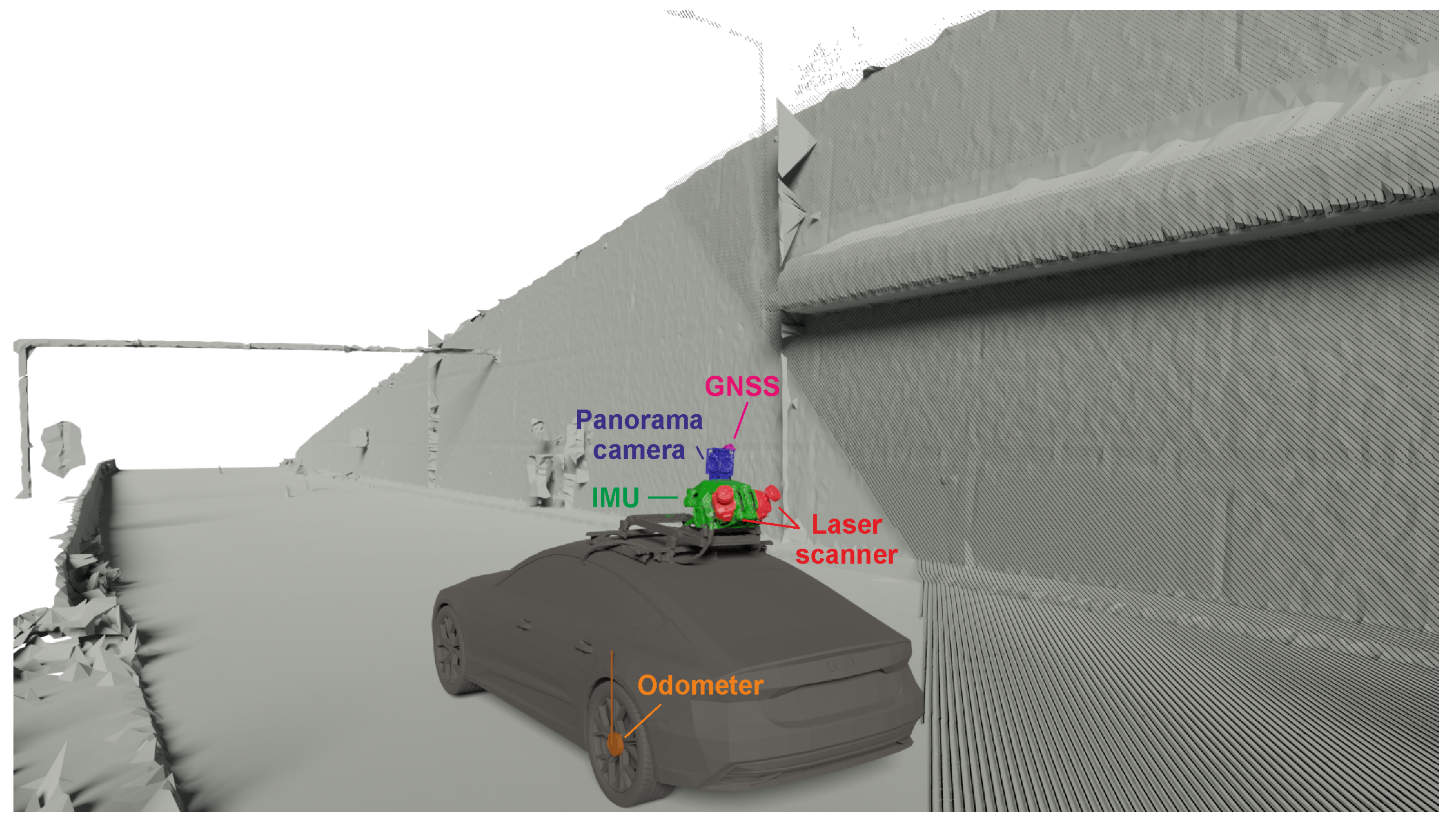
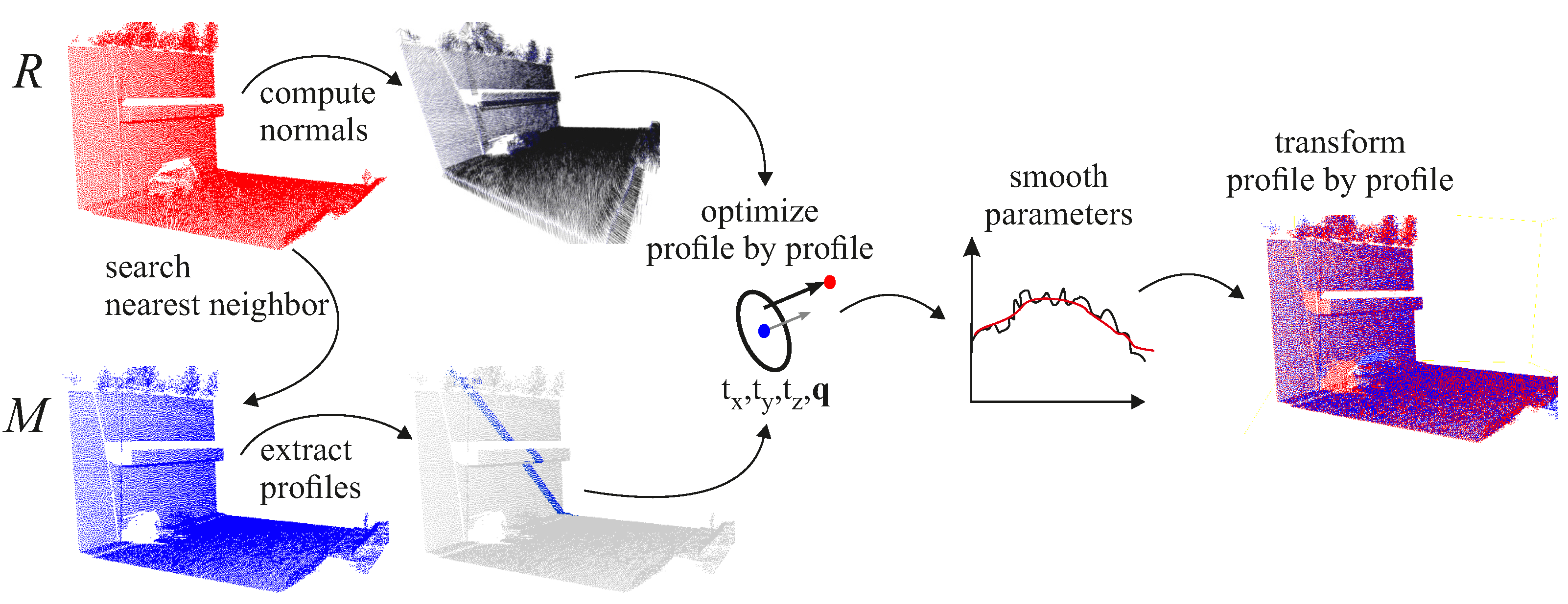
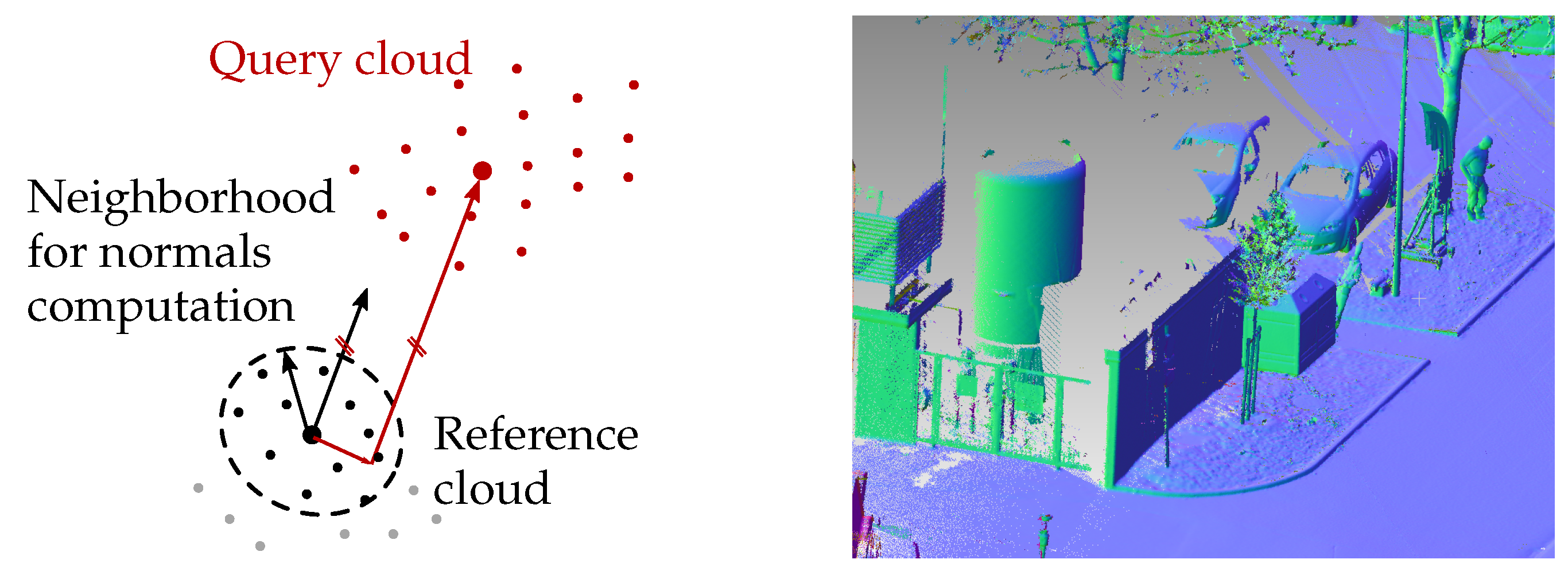
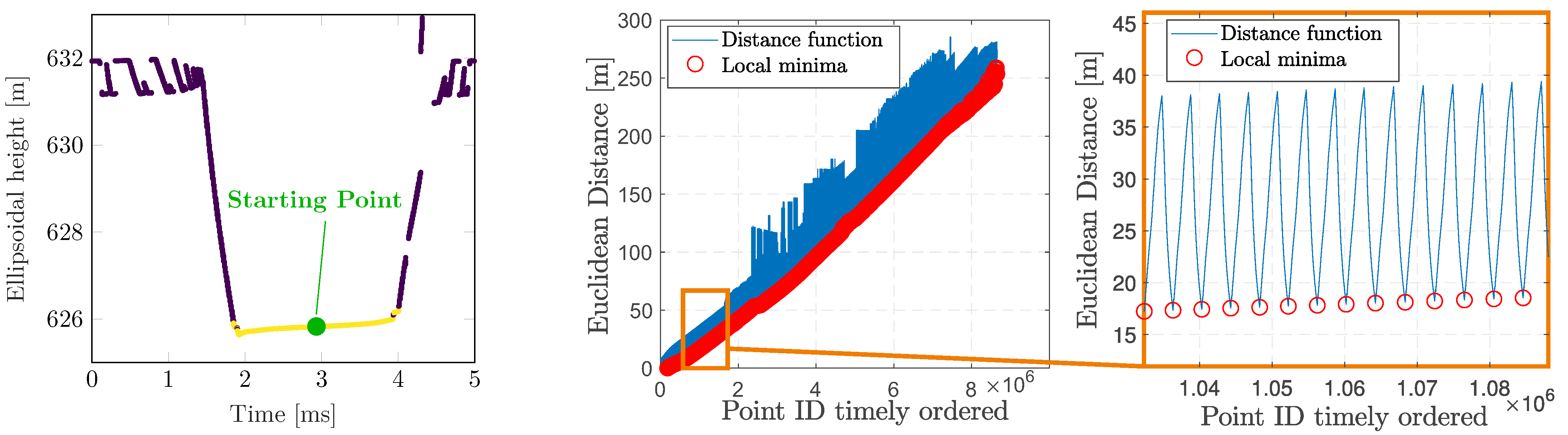
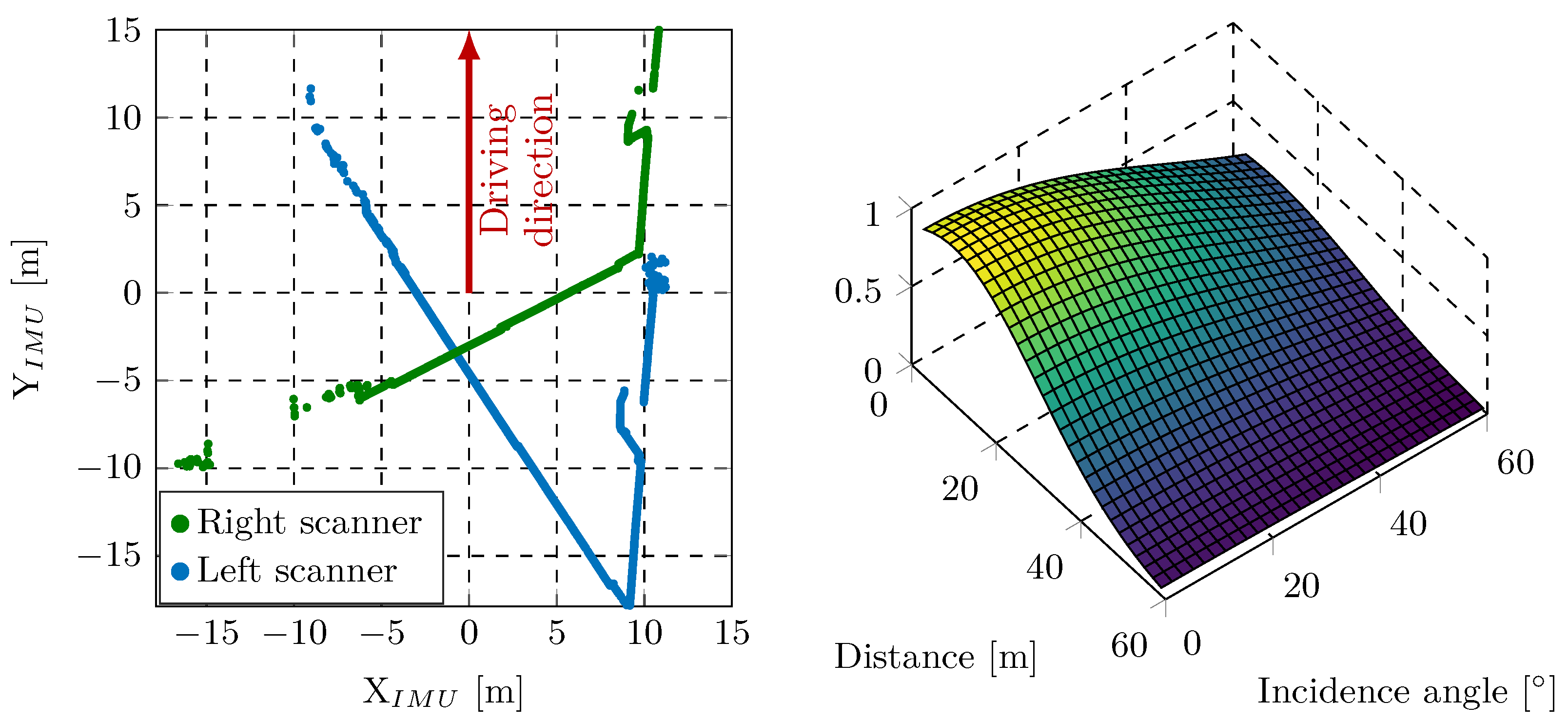
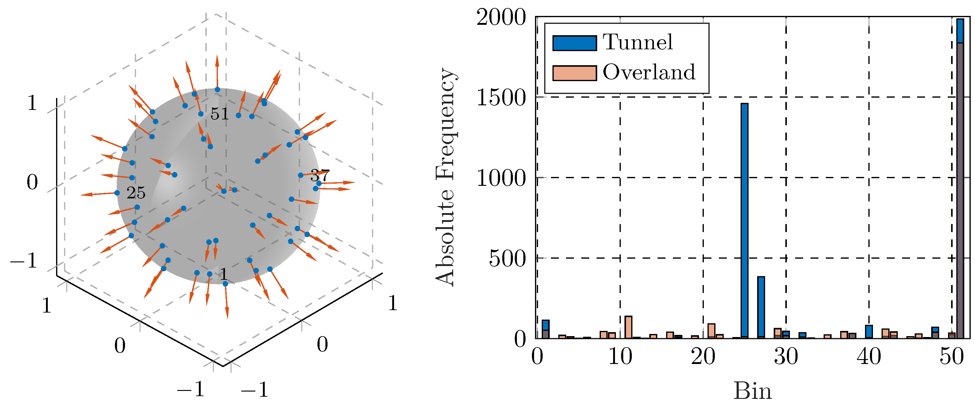
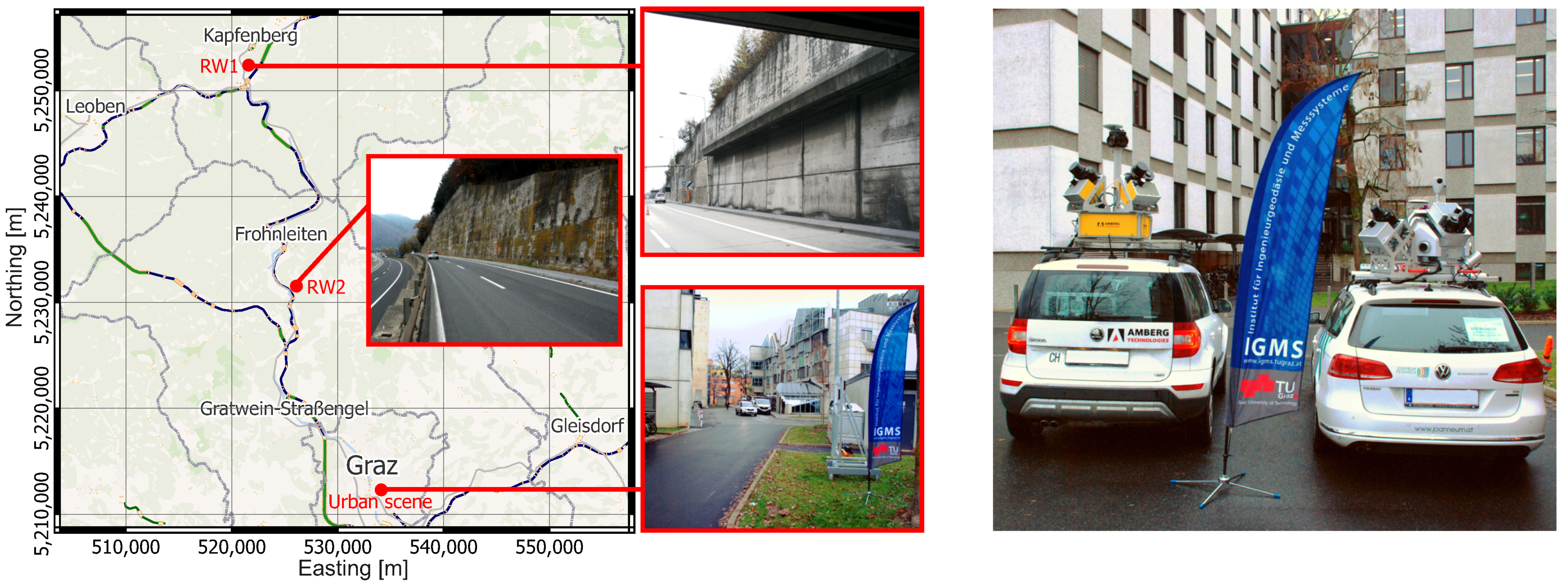
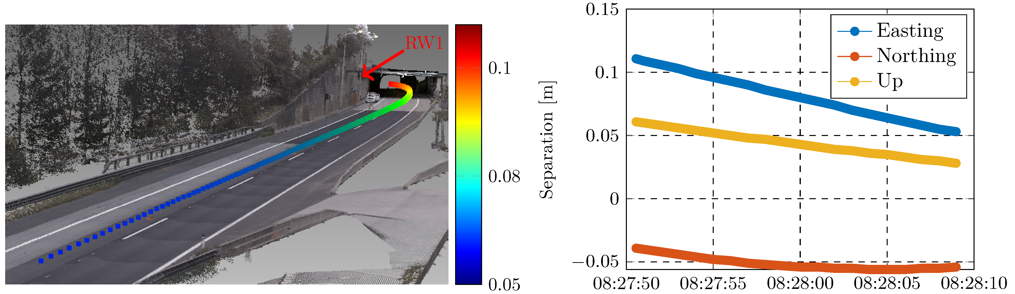
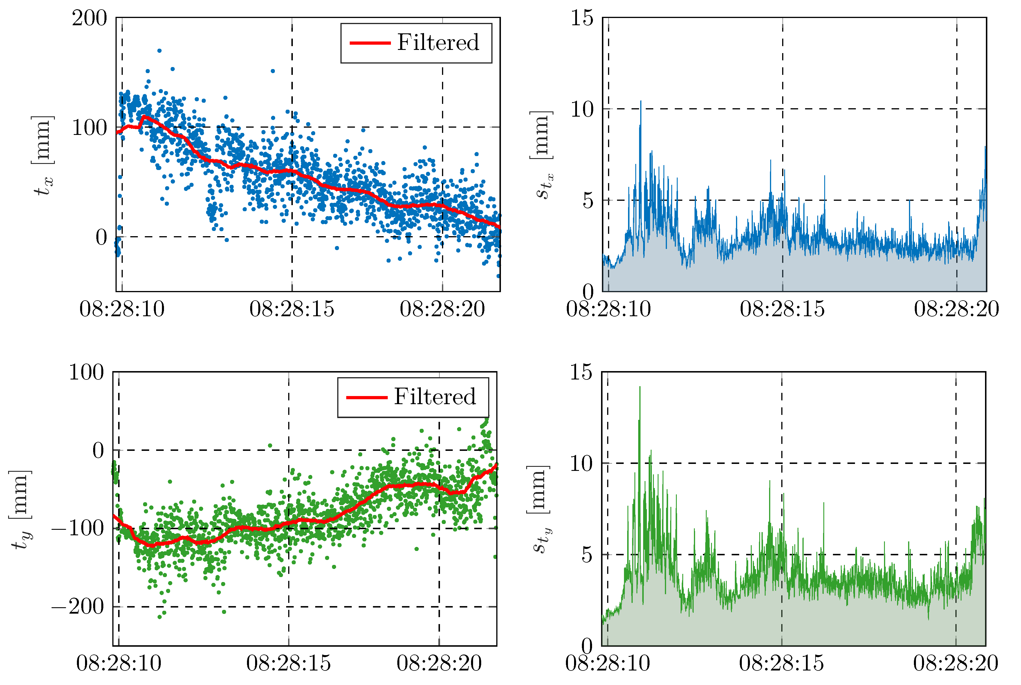
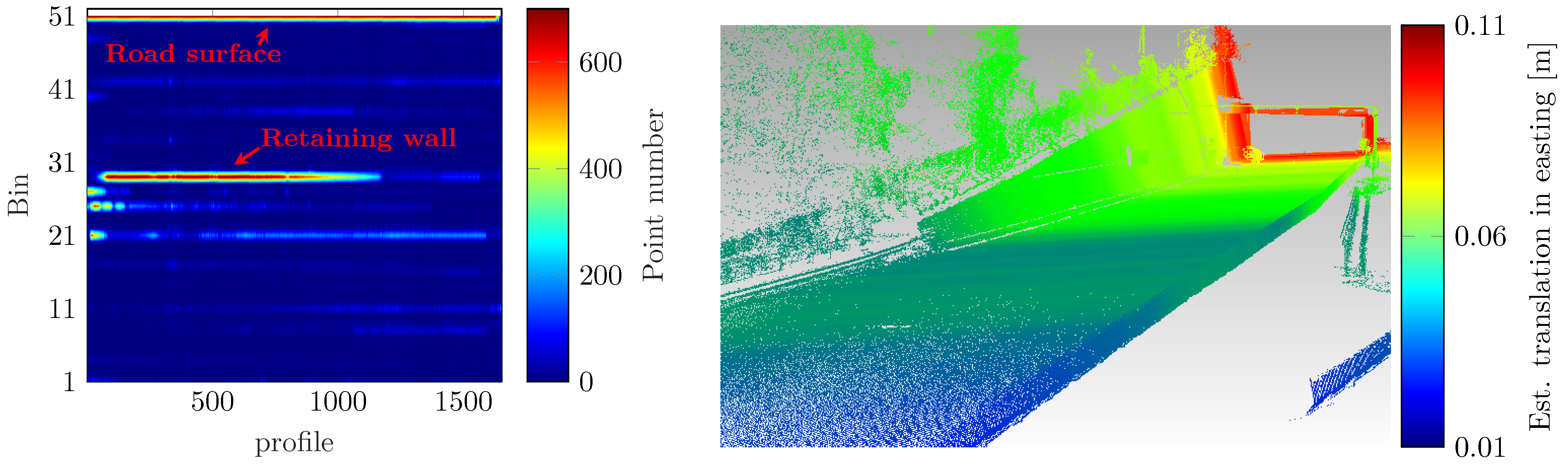
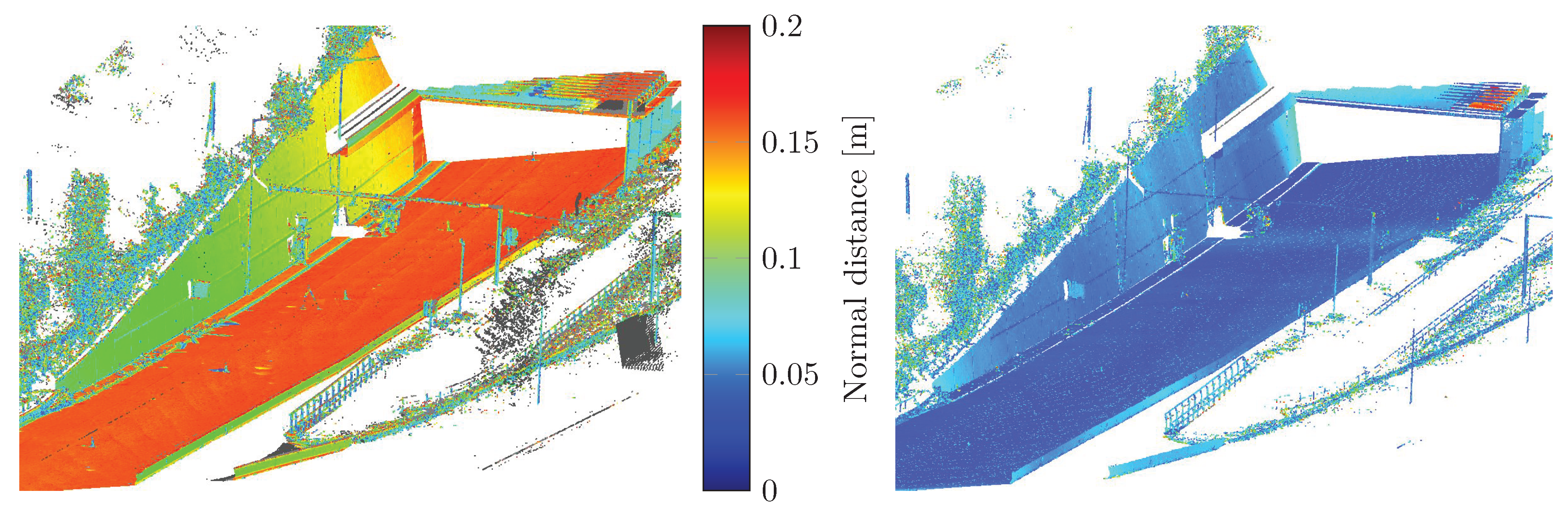
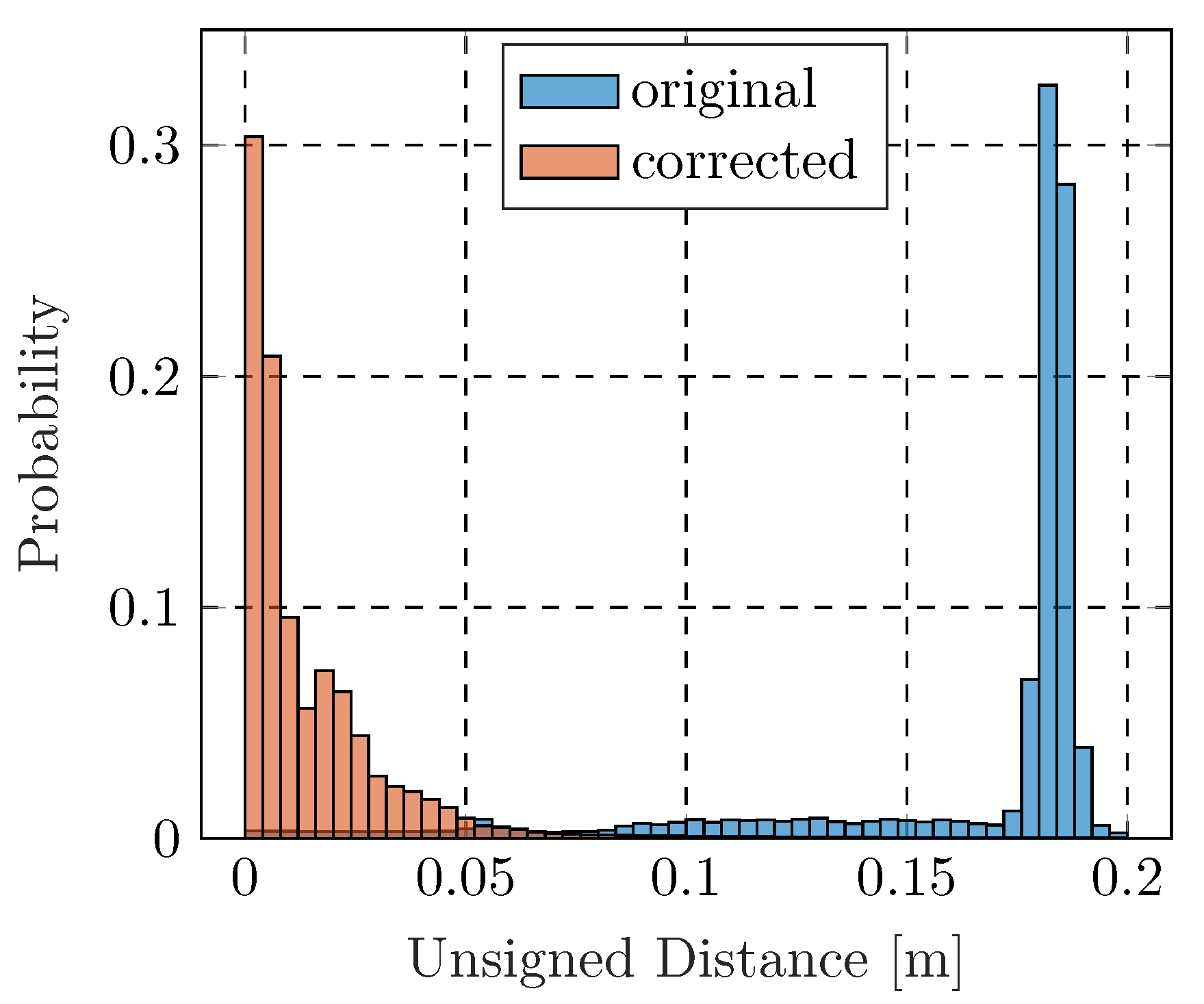
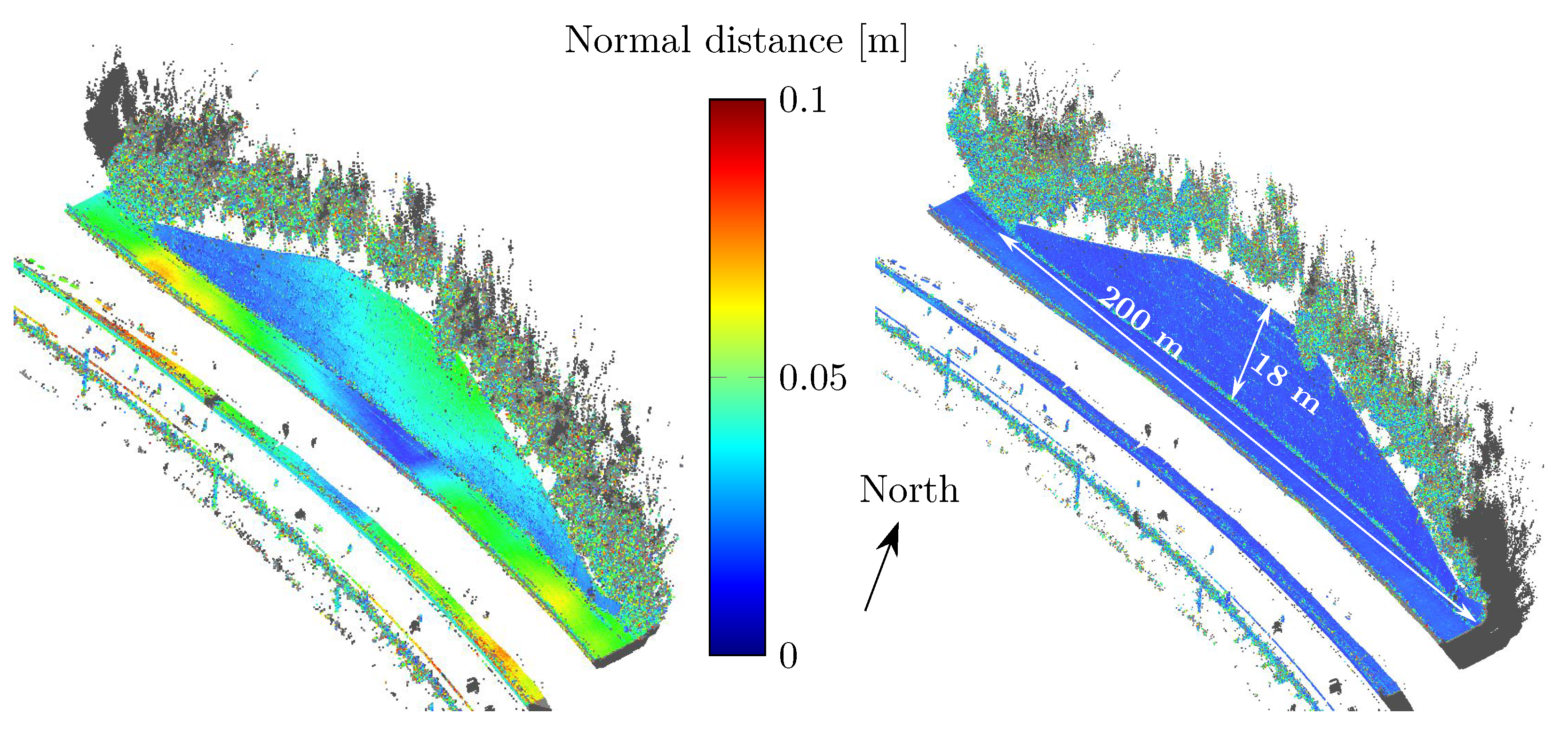
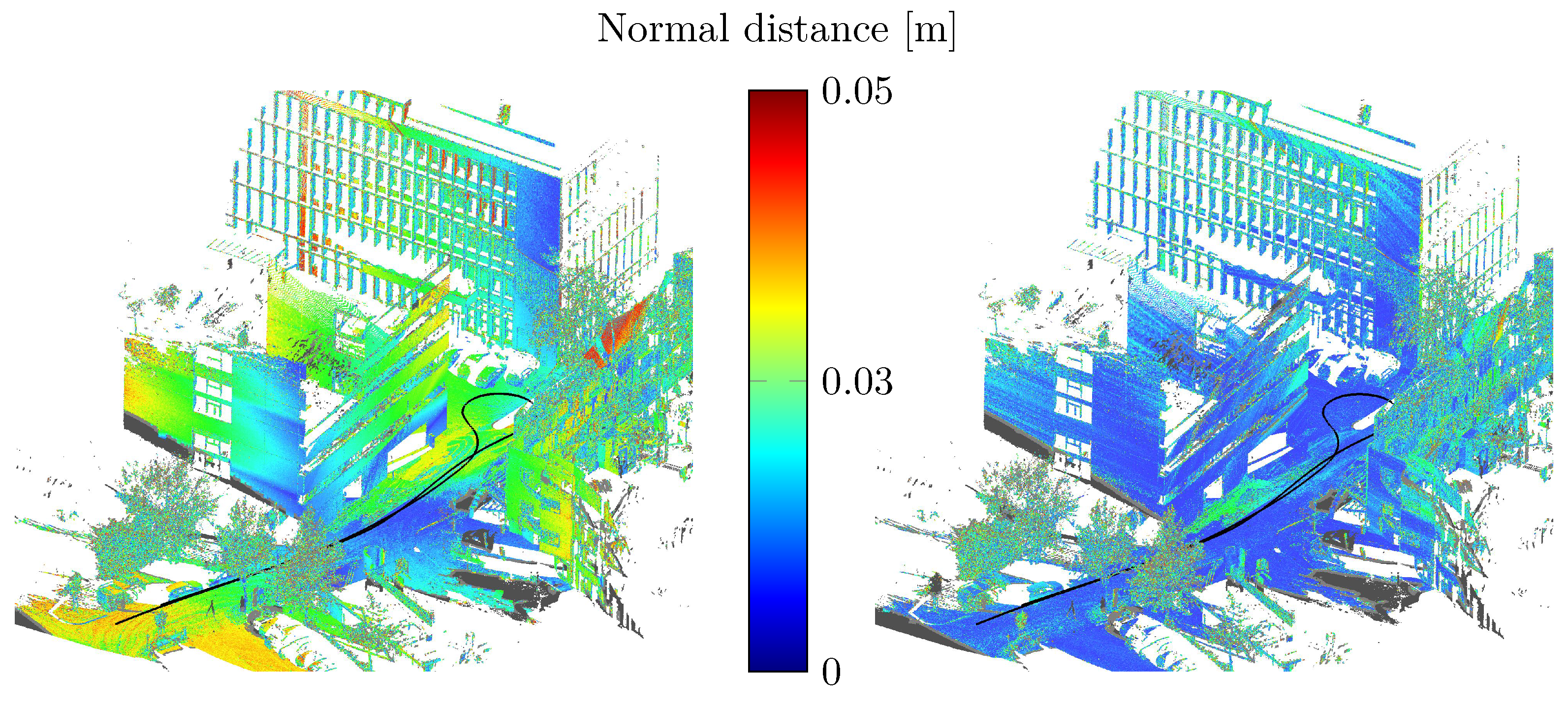
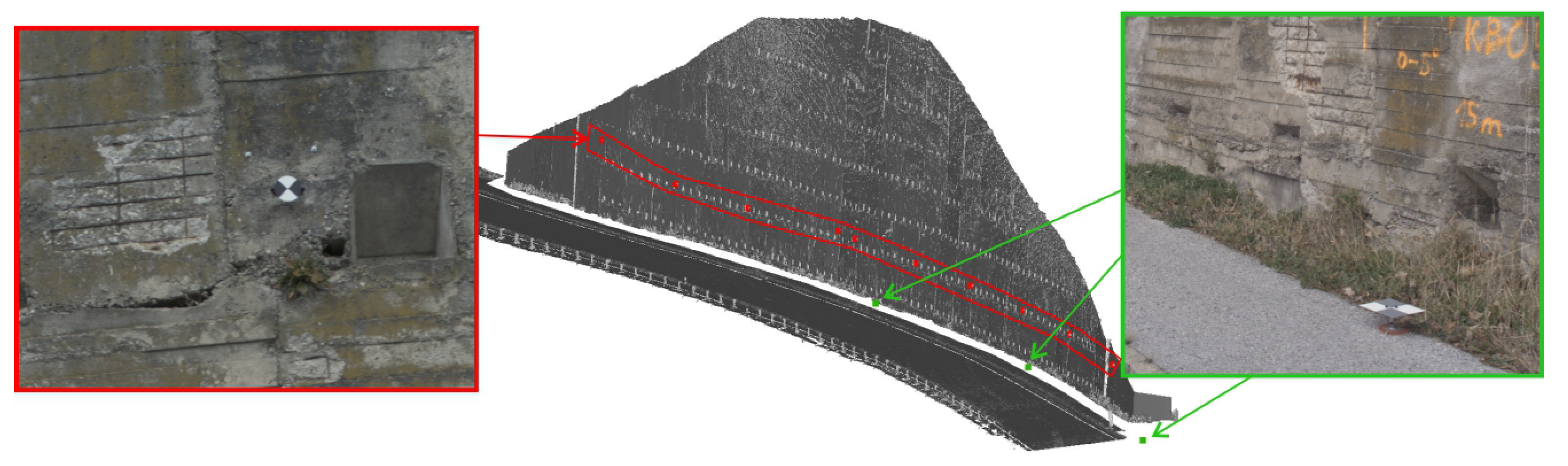
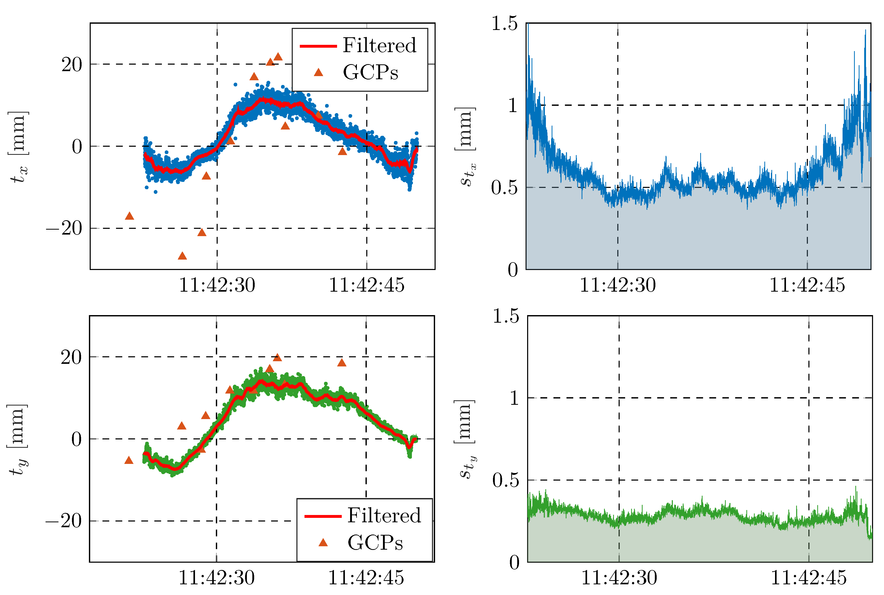
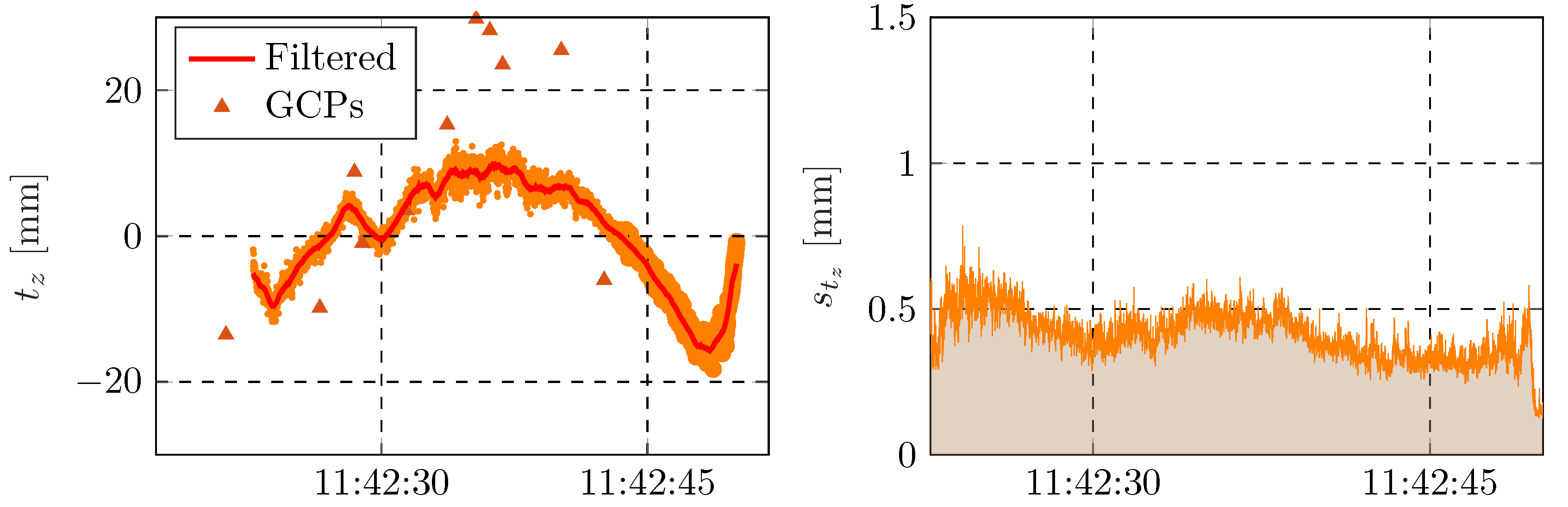
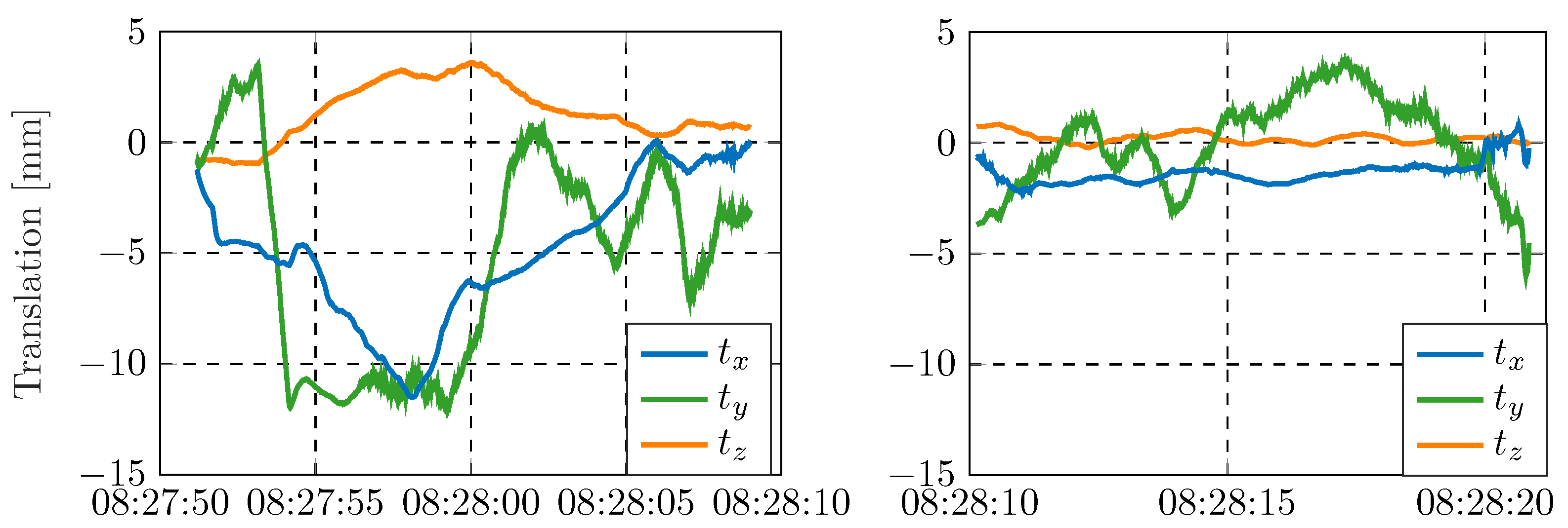
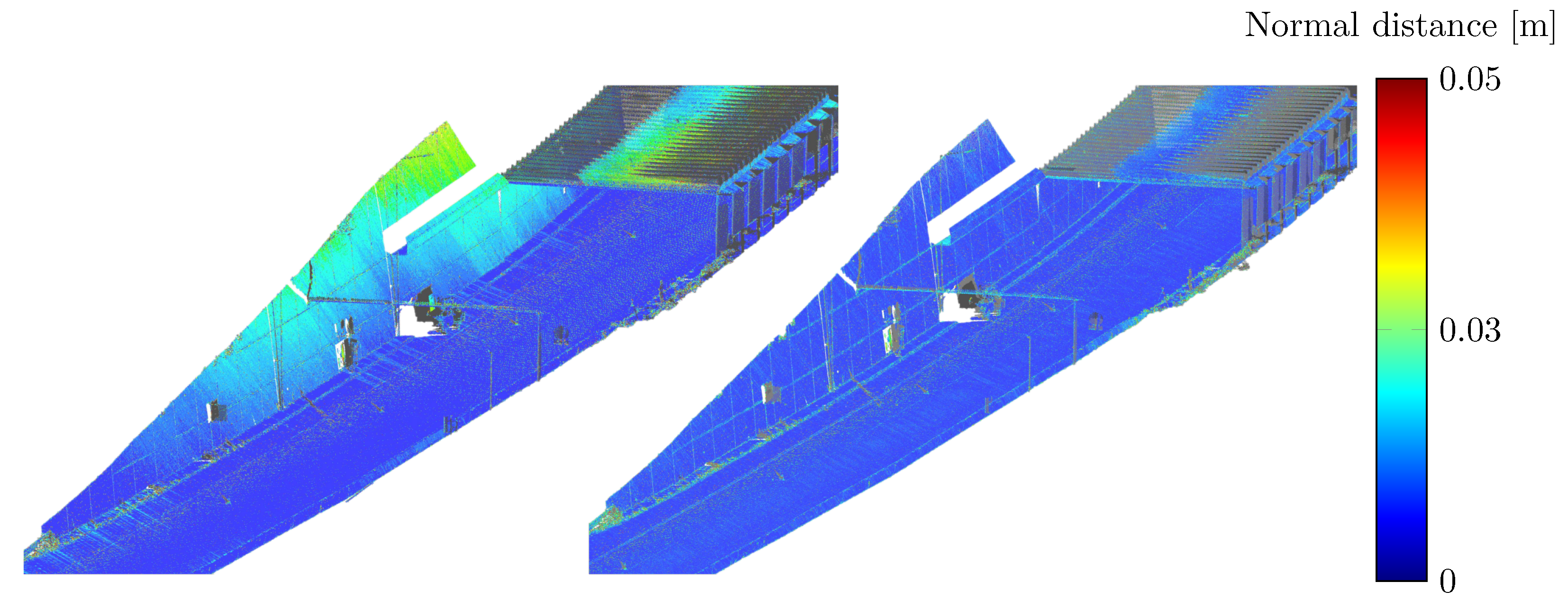
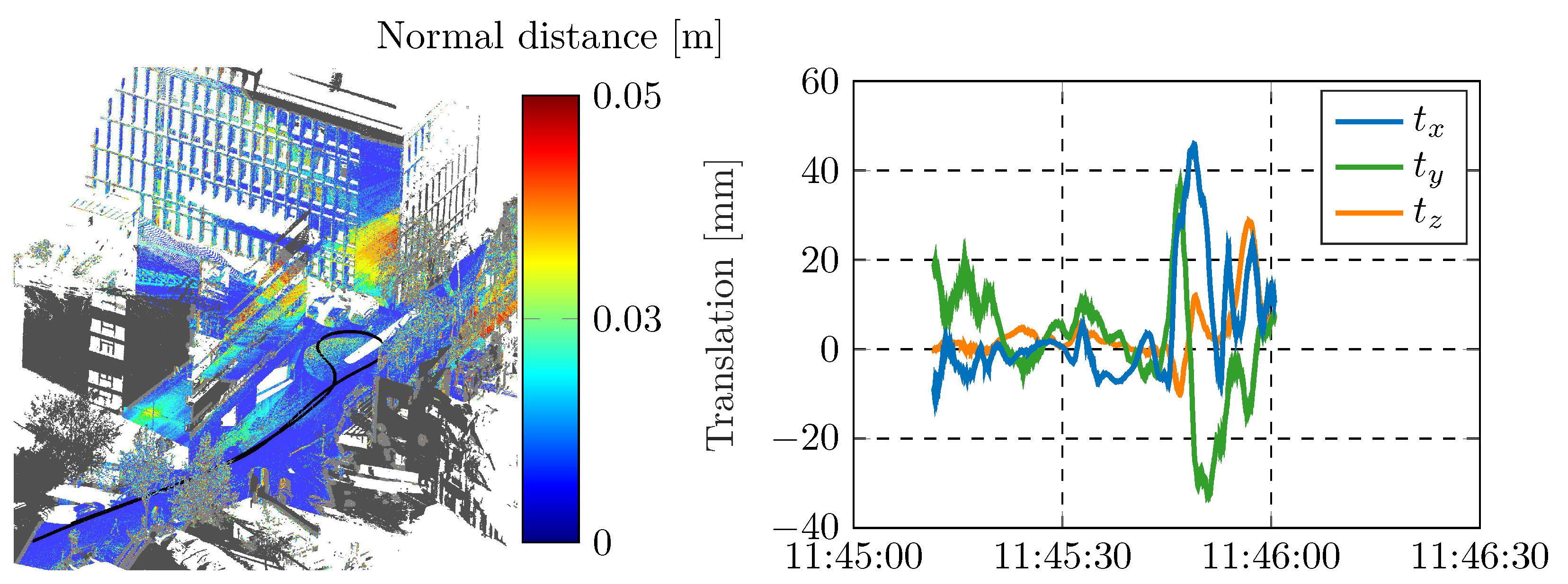
Table 1.
Main differences in the operation of the MLS systems used.
| Road-Scanner 4 | Pegasus:Two Ultimate | |
|---|---|---|
| Scanner rotation speed | 200 Hz | 150 Hz |
| Setup | assembled before operation | fixed |
| Calibration | on-site | during maintenance |
| Scanner configuration | 45/45 | 60/30 |
Table 2.
Statistics of MLS point cloud distances for all combinations before (not-colored) and after correcting RW1 (green-colored): median ± scaled median absolute deviation (MAD) in mm.
Table 2.
Statistics of MLS point cloud distances for all combinations before (not-colored) and after correcting RW1 (green-colored): median ± scaled median absolute deviation (MAD) in mm.
| D | F | H | 402 | 403 | 404 | |
|---|---|---|---|---|---|---|
| D | - | |||||
| F | - | |||||
| H | - | |||||
| 402 | - | |||||
| 403 | - | |||||
| 404 | - |
Table 3.
Statistics of MLS point cloud distances for all combinations before (not-colored) and after correcting RW2 (green-colored): median ± scaled median absolute deviation (MAD) in mm.
Table 3.
Statistics of MLS point cloud distances for all combinations before (not-colored) and after correcting RW2 (green-colored): median ± scaled median absolute deviation (MAD) in mm.
| O | P | Q | R | 802 | 803 | 804 | 805 | |
|---|---|---|---|---|---|---|---|---|
| O | - | 13 ± 14 | 14 ± 16 | 40 ± 12 | 23 ± 15 | 19 ± 15 | 30 ± 6 | 14 ± 9 |
| P | 3 ± 4 | - | 18 ± 15 | 20 ± 16 | 29 ± 21 | 22 ± 14 | 27 ± 16 | 15 ± 13 |
| Q | 2 ± 2 | 3 ± 2 | - | 29 ± 19 | 28 ± 18 | 14 ± 13 | 31 ± 18 | 12 ± 6 |
| R | 5 ± 3 | 2 ± 2 | 4 ± 3 | - | 58 ± 42 | 26 ± 17 | 17 ± 10 | 29 ± 10 |
| 802 | 4 ± 4 | 5 ± 4 | 5 ± 4 | 7 ± 5 | - | 29 ± 26 | 35 ± 28 | 26 ± 21 |
| 803 | 3 ± 3 | 3 ± 3 | 2 ± 2 | 3 ± 3 | 5 ± 4 | - | 29 ± 32 | 11 ± 8 |
| 804 | 3 ± 3 | 2 ± 3 | 3 ± 4 | 3 ± 3 | 4 ± 3 | 4 ± 4 | - | 23 ± 13 |
| 805 | 3 ± 3 | 3 ± 4 | 2 ± 2 | 3 ± 4 | 4 ± 4 | 1 ± 1 | 4 ± 4 | - |
Table 4.
Statistics of MLS point cloud distances for all combinations before (not colored) and after correcting the urban scene (green): median ± scaled median absolute deviation (MAD) in millimeters.
Table 4.
Statistics of MLS point cloud distances for all combinations before (not colored) and after correcting the urban scene (green): median ± scaled median absolute deviation (MAD) in millimeters.
| I | II | III | IV | |
|---|---|---|---|---|
| I | - | |||
| II | - | |||
| III | - | |||
| IV | - |
Publisher’s Note: MDPI stays neutral with regard to jurisdictional claims in published maps and institutional affiliations. |
© 2022 by the authors. Licensee MDPI, Basel, Switzerland. This article is an open access article distributed under the terms and conditions of the Creative Commons Attribution (CC BY) license (https://creativecommons.org/licenses/by/4.0/).
Share and Cite
MDPI and ACS Style
Kalenjuk, S.; Lienhart, W. A Method for Efficient Quality Control and Enhancement of Mobile Laser Scanning Data. Remote Sens. 2022, 14, 857. https://doi.org/10.3390/rs14040857
AMA Style
Kalenjuk S, Lienhart W. A Method for Efficient Quality Control and Enhancement of Mobile Laser Scanning Data. Remote Sensing. 2022; 14(4):857. https://doi.org/10.3390/rs14040857
Chicago/Turabian StyleKalenjuk, Slaven, and Werner Lienhart. 2022. "A Method for Efficient Quality Control and Enhancement of Mobile Laser Scanning Data" Remote Sensing 14, no. 4: 857. https://doi.org/10.3390/rs14040857
Note that from the first issue of 2016, this journal uses article numbers instead of page numbers. See further details here.