
Integrating DMSP-OLS and NPP-VIIRS Nighttime Light Data to Evaluate Poverty in Southwestern China
by
 ,
,
Zhiwei Yong
1, 
Kun Li
2,
Junnan Xiong
3,4,*,
Weiming Cheng
4,
Zegen Wang
1,
Huaizhang Sun
5 and
Chongchong Ye
6 1
School of Geoscience and Technology, Southwest Petroleum University, Chengdu 610500, China
2
PowerChina Sichuan Electric Power Engineering Co., Ltd., Chengdu 610041, China
3
School of Civil Engineering and Geomatics, Southwest Petroleum University, Chengdu 610500, China
4
State Key Laboratory of Resources and Environmental Information System, Institute of Geographic Sciences and Natural Resources Research, Chinese Academy of Sciences, Beijing 100101, China
5
School of Geography and Planning, Sun Yat-sen University, Guangzhou 510275, China
6
State Key Laboratory of Earth Surface Processes and Resource Ecology, Faculty of Geographical Science, Beijing Normal University, Beijing 100875, China
*
Author to whom correspondence should be addressed.
Remote Sens. 2022, 14(3), 600; https://doi.org/10.3390/rs14030600
Submission received: 27 December 2021
/
Revised: 17 January 2022
/
Accepted: 20 January 2022
/
Published: 26 January 2022
(This article belongs to the Special Issue Remote Sensing Imagery for Mapping Economic Activities)
Abstract
:Poverty alleviation is one of the most important tasks facing human social development. It is necessary to make accurate monitoring and evaluations for areas with poverty to improve capability of implementing poverty alleviation policies. Here, this study introduced nighttime light (NTL) data to estimate county-level poverty in southwest China. First, this study used particle swarm optimization-back propagation hybrid algorithm to explore the potential relationship between two NTL data (the Defense Meteorological Satellite Program’s Operational Line Scan System data and the Suomi National Polar-orbiting Partnership Visible Infrared Imaging Radiometer Suite data). Then, we integrated two NTL data at the pixel level to establish a consistent time-series of NTL dataset from 2000 to 2019. Next, an actual comprehensive poverty index (ACPI) was employed as an indicator of multidimensional poverty at county level based on 11 socioeconomic and natural variables, and which could be the reference to explore the poverty evaluation using NTL data. Based on the correlation between the ACPI and NTL characteristic variables, a poverty evaluation model was developed to evaluate the poverty situation. The result showed the great matching relationship between DMSP-OLS and NPP-VIIRS data (R2 = 0.84). After calibration, the continuity and comparability of DMSP-OLS data were significantly improved. The integrated NTL data also reflected great consistency with socioeconomic development (r = 0.99). The RMSE between ACPI and the estimated comprehensive poverty index (ECPI) based on the integrated NTL data is approximately 0.19 (R2 = 0.96), which revealed the poverty evaluation model was feasible and reliable. According to the ECPI, we found that the magnitude of poverty eradication increased in southwest China until 2011, but slowed down from 2011 to 2019. Regarding the spatial scale, geographic barriers are a key factor for poverty, with high altitude and mountainous areas typically having a high incidence of poverty. Our approach offers an effective model for evaluation poverty based on the NTL data, which can contribute a more reliable and efficient monitoring of poverty dynamic and a better understanding of socioeconomic development.
1. Introduction
Poverty is a long-term worldwide predicament and a main cause of instability for society [1]. It is estimated that 735.9 million people remained in poverty ($1.90 per day) during 2015. Poverty eradication is the primary goal of the Sustainable Development Goals (SDGs) set forth by the United Nations. Therefore, poverty reduction has become a vital task faced by many countries [2]. China has implemented huge amounts of work for poverty alleviation and has achieved remarkable results. By the end of 2020, all the 770 million Chinese rural population living below the poverty line were lifted out of poverty, and region-wide absolute poverty was resolved. However, imbalanced and inadequate development are still urgent issues for China, which are barriers to China’s sustainable development. Meanwhile, consolidating achievements of poverty alleviation also will be the next priority. There is still a long and tough road to completely eliminate poverty in China [3]. Hence, accurately and objectively evaluating and monitoring poverty level and development situations are crucial for governments to continue the strategy of rural vitalization and promote balanced development.
Traditionally, statistics data provides the main basis of poverty level evaluation and analysis. In the beginning, poverty is considered as an economic phenomenon [4], thus poverty measurement and determination is mainly based on the single economic dimension [2], and census data such as gross domestic product (GDP) is the most prominent indicator [5]. However, GDP cannot be treated as a sole measure of a country’s well-being because it is unable to express many components related to individual and social well-being [6]. With the development of the poverty concept, poverty studies have turned to a multidimensional assessment that involves not only economic but also natural, human and other aspects [7]. Multidimensional indicators are often more accurate than using a single economic dimensional [8], therefore many studies use this way to identify regional poverty levels and have obtained quite reasonable results [8]. However, more dimensions also mean higher requirements for data integrity. Besides, the time-sensitivity of data limits these traditional methods based on statistic or survey data. Because of the high cost, most existing statistics are updated by census or survey at long intervals [9], and detailed poverty-related data still needs to be provided between the intervals [10].
Satellite remote sensing data, especially nighttime light (NTL) imagery, offers a timely, objective and consistent way for direct observations about human activities [11]. Compared to other satellite products, NTL data has a distinct advantage in quantifying human activities [12], and it has been widely used to monitor socioeconomic dynamics [13], such as urbanization [14], population [15], GDP [16], electricity consumption [17] and so on. Therefore, NTL data correlates closely with poverty distribution as well. The most used NTL data sources include the Defense Meteorological Satellite Program’s Operational Line Scan System (DMSP-OLS) and the Suomi National Polar-orbiting Partnership Visible Infrared Imaging Radiometer Suite (NPP-VIIRS) Day-Night Band. Both datasets have been utilized in poverty analysis. For the sake of simplicity and convenience, some studies accomplish poverty level evaluation by exploring the correlation between NTL data and poverty indices [18]. However, most of these studies tended to focus on single NTL feature, which may cause the omission of important information that can be useful for exploring poverty [19]. Meanwhile, the commonly regression models that relate NTL to poverty indices might not work well without a huge prior knowledge of the potential relationship between inputs and outputs [11]. Therefore, some other scholars utilized classification features of NTL data, and adopted machine learning approaches to identify the poor counties [11]. These previous studies provide useful thoughts for poverty research based on NTL data, but there are some uncertainties that poverty probability obtained from these classification approaches. The previous training model is based on the output of “poor counties” as “1” and “non-poor counties” as “0”, without linking NTL to the real socioeconomic information [19], but only relying on the night light itself to interpolate between 0 and 1, which can hardly reflect the multidimensional characteristics of poverty. In addition, poverty is a long-term dilemma, but the applications of NTL data in poverty analysis are hindered by the sensor differences and temporal coverage differences of different NTL products [12].
The DMSP-OLS NTL dataset provides a continuous time series during the period 1992–2013, while the NPP-VIIRS NTL product runs from 2012 to the present. As the result of the evident inconsistency between the two data sources, however, it is difficult to directly apply multi-source NTL data for long-term studies [20]. Therefore, it is essential to connect the DMSP-OLS and NPP-VIIRS NTL to construct a continuous time series NTL dataset for facilitating long-term research. There have been some studies attempting to integrate NTL from both sources for extending NTL data. For example, Zhu et al. [21] attempted to integrate the DMSP-OLS and NPP-VIIRS NTL datasets at the provincial level using the relationship of power function, and Zhao et al. [22] achieved this with a quadratic polynomial model at the level of county. However, these datasets generated at the administrative level have limited application at a finer scale. Meanwhile, the applicability of current approaches still suffers from some limitations, especially the limited accessibility of datasets [23], regional limitations of methods et al. [24] Moreover, the widely-used fixed regression model [25] may fail to explain the undefined mechanisms correlating the two NTL datasets and lead to mismatch. For the well-acknowledged NTL data [26], whose accuracy is still limited by saturation, this may affect the final results obtained in this study. On the contrast, back propagation (BP) artificial neural network (ANN) is an efficient multilayer feedforward neural network with wide applicability. However, there are some inherent problems in BP algorithm, such as trapping in local minima easily and the low convergent speed [27]. Particle swarm optimization (PSO) algorithm has a great ability to obtain the global optimistic results [28], which is also adopted to improve the performance of BP algorithm. Hence, in the study, by combining the PSO with the BP, a PSO-BP hybrid algorithm was used to construct the ANN for exploring the potential relationship between the DMSP-OLS and NPP-VIIRS data.
Hence, the major objectives of this study are: (1) to integrate DMSP-OLS and NPP-VIIRS NTL data at the pixel level based on the PSO-BP hybrid algorithm, and establish a consistent time-series of NTL dataset from 2000 to 2019; (2) to establish an efficient method for poverty evaluation based on NTL feature variables by exploring the relationship between them and an actual comprehensive poverty index (ACPI), and implement poverty evaluation in southwestern China from 2000 to 2019 based on the consistent NTL dataset; (3) to analyze the spatiotemporal variations of regional poverty in southwestern China from 2000 to 2019.
2. Study Area and Data
2.1. Study Area
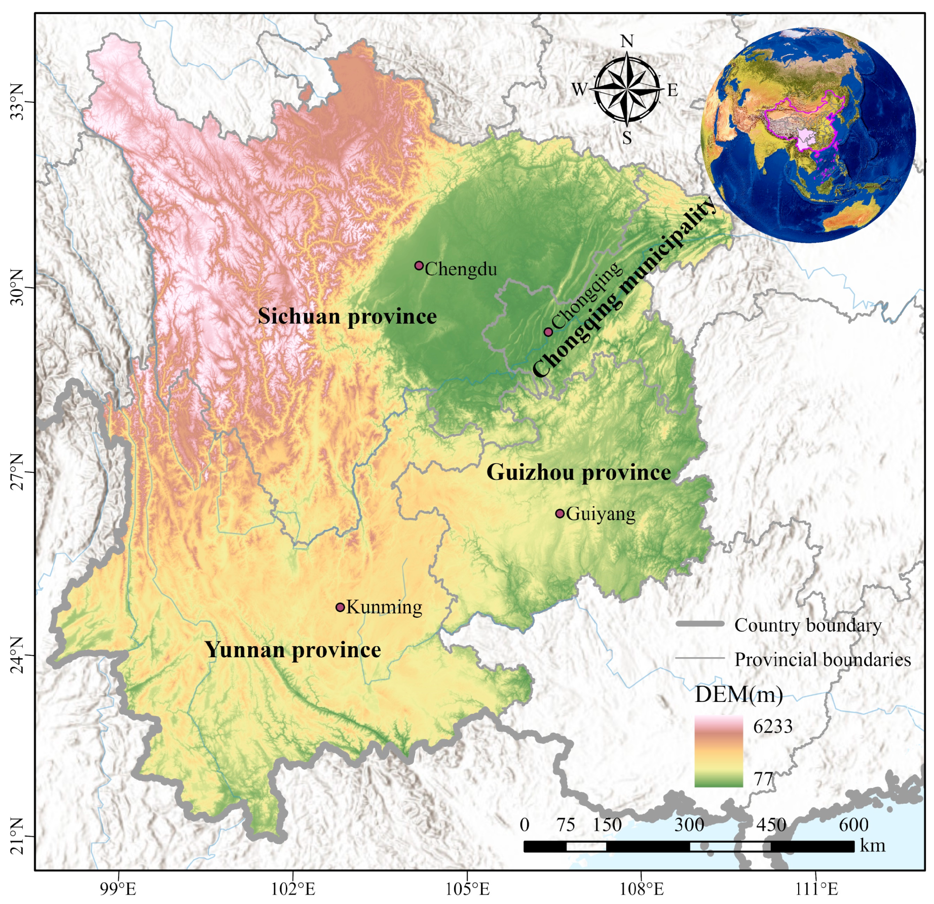
In this study, southwestern China is defined as the area consisting of four provinces: Sichuan, Chongqing, Yunnan and Guizhou, which includes 438 county-level divisions (Figure 1). There is a complicated topography which mainly consists of four topographic sorts: mountains, hills, plains, and plateaus. At the end of 2019, the total population of southwestern China was 199.8 million, but its distribution is uneven. Its economic development is also polarized: the total GDP of the Southwestern China reached 11.02 trillion RMB, but 44.29% is accounted by Sichuan alone; only the per capita GDP of Chongqing (75,828 RMB) is higher than the national average (70,892 RMB), while the rest (55,774 RMB for Sichuan, 47,944 RMB for Yunnan and 46,433 RMB for Guizhou) are far below the average, which also indicates that the per capita economic level of the study area is relatively backward compared with other regions in China. Meanwhile, more than half of the counties in southwestern China have been designated as the national poverty alleviation counties. Therefore, it is a representative region for poverty alleviation (Figure S1).
The sample areas came from 38 counties in Chongqing, and the others were utilized as estimation areas. Chongqing has not only been undergoing rapid economic development, but is also suffering from an apparent regional inequality and poverty [3,8]. Therefore, the sampled areas can be considered as the representative region for poverty evaluation in study area.
2.2. Data and Pre-Processing
2.2.1. Data Sources
The DMSP-OLS and NPP-VIIRS NTL products of this paper are used as main NTL data sources. The Version 4 DMSP-OLS data from 1992 to 2013 were provided by Earth Observation Group, Payne Institute for Public Policy, Colorado School of Mines (https://eogdata.mines.edu/products/dmsp/, accessed on 20 April 2021). These NTL data are composed of observations from different satellites and include lights from cities, and other continuous illuminations, but discard transient lights such as fires and filter out background noise. The DMSP-OLS NTL data has a spatial resolution of 30 arc seconds, and a digital number (DN) value range of 0–63. The stable light product has been widely used, however, there are some inherent deficiencies, such as brightness saturation, incomparability and inconsistency [29]. The stable NTL data from 2000 to 2013 are utilized in this study.
The NPP-VIIRS NTL data since 2012 were also obtained from Earth Observation Group, Payne Institute for Public Policy, Colorado School of Mines (https://eogdata.mines.edu/products/vnl/, accessed on 22 April 2021), and the Vision 1 monthly “VIIRS Cloud Mask” data from April 2012 to December 2019 are selected in this study. Compared to DMSP-OLS NTL data, NPP-VIIRS NTL data have a higher spatial resolution (15 arc-seconds), a wider range of radiometric detection, and are exempt from saturation problems of brightness. Meanwhile, negative values and outliers remain in raw NPP-VIIRS NTL data.
Besides, the data sources employed in this study also covered administrative boundary data, socioeconomic statistical data and DEM data. The description of each data sources is given in Table 1.
2.2.2. Data Pre-Processing
As mentioned above, there are several differences between the DMSP-OLS data and NPP-VIIRS data, therefore both datasets need pre-processing before they can be used in further studies.
Firstly, DMSP-OLS NTL data were processed with following two major steps: (1) all NTL data were masked by administrative boundaries of southwestern China and resampled to the resolution of 1000 m × 1000 m with a Albers Conical Equal Area projection; (2) an invariant region method [22], intra-annual correction [21] and inter-annual correction [30] were adopted to reduce discontinuities, incomparability, and brightness saturation effect, improving the consistency and comparability of DMSP-OLS time series [31]. These methods have been shown to be convenient and effective in previous studies [30,32].
Secondly, to reduce the negative factors in monthly NPP-VIIRS NTL data, four major steps [31] were implemented: (1) masking extracted from corrected DMSP-OLS data were applied to remove background noises of NPP-VIIRS data, while replacing negative values with zero; (2) assigning the maximum DN value among Beijing, Shanghai, Guangzhou and Shenzhen to be the threshold value to filter abrupt brightness in each monthly NTL imagery, and Chengdu, Chongqing, Kunming and Guiyang were also utilized as supplementary to deal with some unresolved pixels. (3) eliminating the effect of stray light pollution [33], monthly NPP-VIIRS NTL data except from April to August were used to synthesize the annual data. (4) clipping, resampling and re-projecting annual NPP-VIIRS NTL data in the same way.
3. Methodology
The methodological workflow implemented in this study is schematically shown in Figure 2.
3.1. Integration of DMSP-OLS and NPP-VIIRS NTL Data
The procedures of data pre-processing allowed the DMSP-OLS correction data (2000–2013) and the NPP-VIIRS correction data (2012–2019) to be obtained. However, they were still not comparable due to the considerable differences in radiometric properties between sensors. To facilitate the longer-term continuous application of NTL data and extend temporal series, the two sources need to be inter-calibrated and integrated. Hence, a convenient method was proposed in this study to extend NTL data by implementing the conversion from NPP-VIIRS data to DMSP-OLS data at the pixel scale.
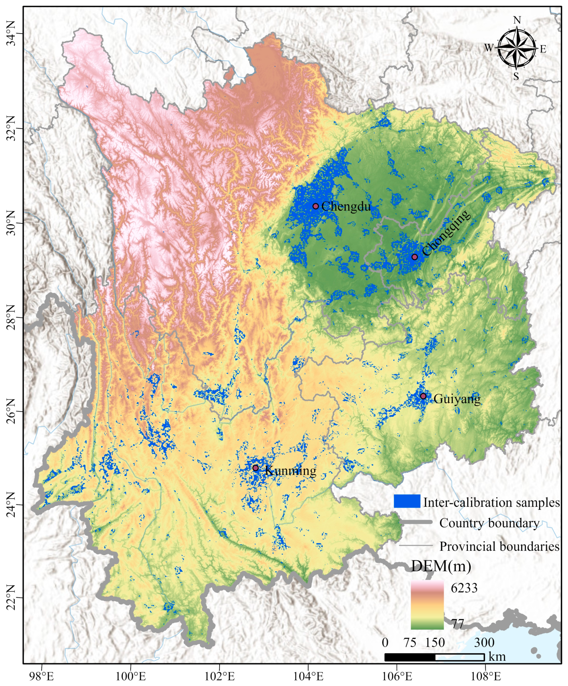
The overlap period (2012 and 2013) of two datasets provided the basis of NTL in-tegration. Earlier studies [30] commonly constructed integration models based on the cumulated total DN values (TDN) of regions, however, which may be general and lead to deviation in some regions [31]. Therefore, considering that the calibration site designed especially for NTL was unavailable in the world [34], samples for inter-calibration were selected to capture conversion parameters in this study. Consistent with previous research [35], the coefficient of variation () with a threshold of 20%, which was assumed to represent the stable NTL radiation, was applied to select suitable inter-calibration samples within the following three processes: (1) calculating the values of all pixels in DMSP-OLS raster and NPP-VIIRS raster using 3 × 3 window; (2) extracting the intersection of areas in DMSP-OLS and NPP-VIIRS with values less than 20%, which were seen as temporally and spatially stable; (3) composing the inter-calibration samples with positive pixels in intersection areas. The is defined as in Equation (1). Given the incompleteness of NTL in 2012 [25], the inter-calibration samples in 2013 were used in this study, and the distribution of the inter-calibration samples across southwestern China is shown in Figure 3.
where is the standard deviation of pixels values in a 3 × 3 window; is the mean of pixels values in a 3 × 3 window.
Next, a logarithmic transformation was also applied to NPP-VIIRS (Log_V), and the pixel values of Log_V and DMSP-OLS within the inter-calibration samples in 2013 were extracted as the basic input and output of the ANN, respectively. Referring to the previous approach [32], the central geographic coordinates (X and Y) and the area of each county (Area) to which pixels belong were selected as supplementary input parameters to improve accuracy. Then, 51,052 samples were obtained, and they were randomly divided to training samples and testing samples with a proportion about 9:1. Afterwards, the network was trained by PSO and BP algorithm with the training procedure which corresponds with previous studies [36]. The related parameter settings of PSO-BP algorithm are shown in Table S1 [37].
In addition, three extra ANNs and five fixed regression models (linear, quadratic polynomial, log function, power function and exponential function) were developed in 2013, further analyzing the effectiveness of the proposed method. The basic descriptions of those ANNs are shown in Table 2.
3.2. Construction of ACPI
Poverty is a multidimensional phenomenon that involves many aspects related to human development and the natural environment, evaluating multidimensional poverty based on statistics has been widely adopted by scholars [38]. Therefore, the multidimensional poverty index is employed as an indicator of regional multidimensional poverty. Because of the data availability, referring to the Sustainable Livelihoods Framework proposed by the Department for International Development [39] and previous studies [40,41], financial assets represent the overall economic income of the county and the average income level of residents. The social assets include the exercise and protection of the rights in livelihood, such as personal development, education, and medical treatment. Natural assets can affect livelihood and development strategies. Therefore, 11 socioeconomic and natural variables from financial, social and natural assets have been extracted to establish a multidimensional poverty evaluation system for the study area. An ACPI from this evaluation system could be the reference to explore the poverty evaluation using NTL data, as listed in Table 3.
Then, the annual was calculated for each county based on the following equation:
where indicates the value of the ith county in a particular year, wj denotes the weight of the jth index, and the xij denotes the standard value of the jth index in ith county in the same year.
The dimension and order of magnitude of the original data of each indicator are different, so data standardization processing is required before data analysis to eliminate the impact of different dimensions. Then, the entropy method was used in this study to determine the weight of indices (Table 3), and the corresponding process were consistent with the work of Fang and Ma [42] and Li et al. [38]. Therefore, the ACPIs from 2000 to 2019 in 38 sample counties were obtained. Theoretically, the average level of regional multidimensional poverty can be represented by the calculated value. We use the natural discontinuous classification method to classify into five categories: extremely low, low, medium, high and extremely high. The advantage of this classification method is that it is less influenced by human influence, produces minimal differences within categories and maximum differences between categories [22].
3.3. Evaluating Poverty Based on NTL Data
The basic assumption of this study is that NTL information can be used as an accurate and beneficial proxy for analyzing the regional poverty, which also has been suggested by the signs of existing studies [8]. And the poverty evaluation model was built by exploring the relationship between and NTL feature variables, and to evaluate the multidimensional poverty in southwest China. According to the actual poverty alleviation policies in China, the county-level administrative districts are basically used as poverty alleviation targets. Next, a single pixel cannot contain more NTL information (Table 4). Hence, this study evaluated poverty at county-level based on the integrated NTL data.
At first, referring to the approaches in related studies [40], 12 NTL features which included not only the simple statistical features, but also these spatial features contained meaningful information in NTL images. These indices describe the central tendency, spatial patterns and degree of dispersion of NTL distribution in each county, thus, it comprehensively reflects the differences and similarities among counties in different aspects. Table 4 provides a description of a total of 12 NTL feature variables for poverty evaluation.
Then, the results of the correlation analysis showed that the multidimensional poverty level was positive correlated with the 1–6 and 8–12 characteristic variables, and negative correlated with F7 at the 1% significance level (Table 5), which also indicated the rationality of extracted NTL feature variables in this study. Consequently, all the selected NTL features could be used to construct the model of poverty evaluation.
Finally, considering the complexity of poverty and the lack of prior knowledge connecting poverty and NTL features, the PSO-BP algorithm were also utilized to fit and train the model. Concretely, based on the data of sample areas, we selected a total of 12 NTL feature variables as the input parameters, and the estimated CPIs () were the output parameters.
3.4. Accuracy Assessment
It is necessary to carry out an accuracy assessment to analyze the effectiveness of the fitting model. Besides the correlation coefficient (r) and determination coefficient (R2), relative error (), and mean relative error () were employed to evaluate accuracy. They are defined as:
where is the estimated ; is the value of ; n is the number of years.
4. Results and Discussion
4.1. Results of NTL Integration
4.1.1. Integration Model
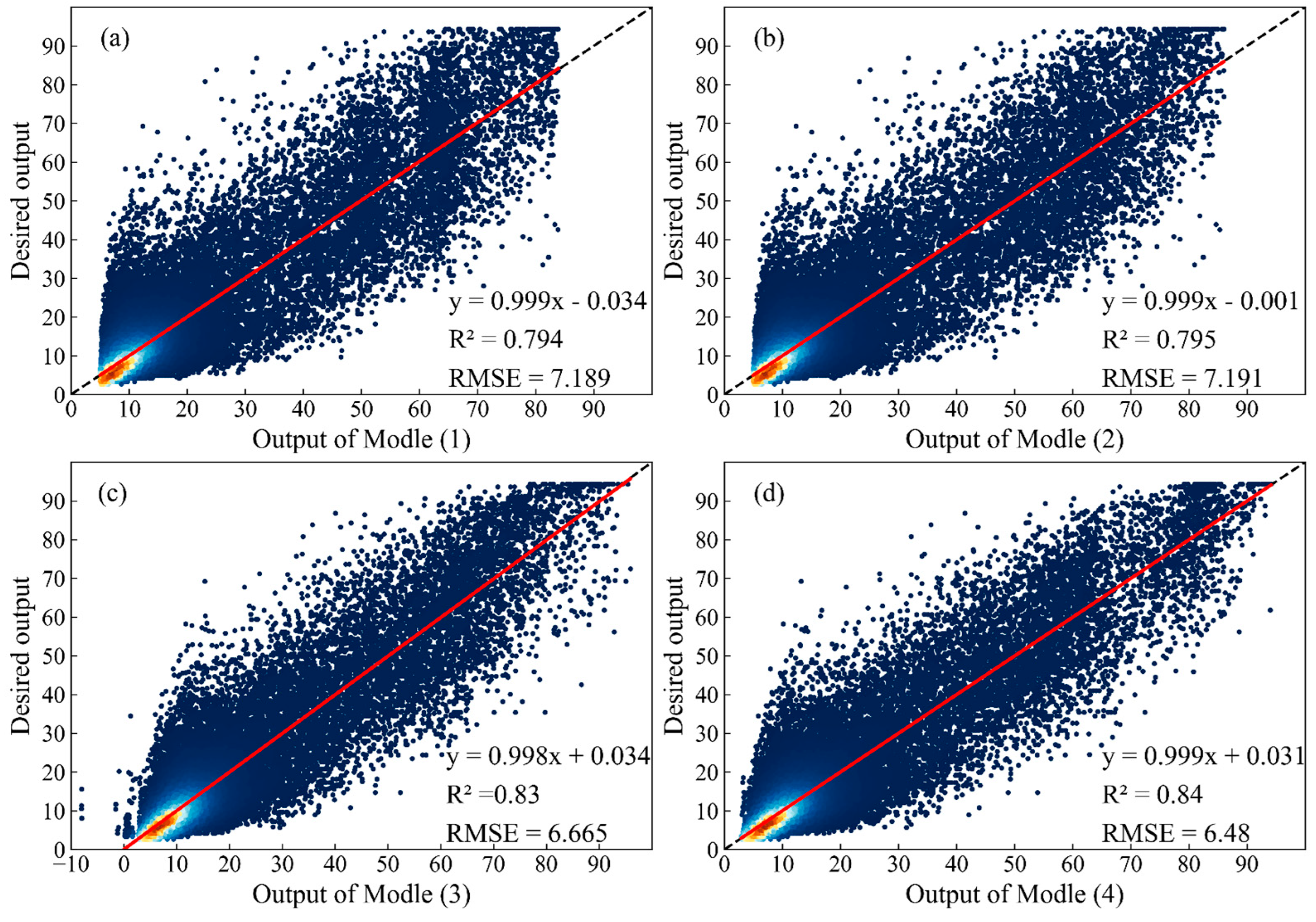
As mentioned above, four ANNs model (Table 2) were trained for transforming the NPP-VIIRS data into simulated DMSP-OLS data, and the model results are presented in Figure 4. The slope of those fitted lines was extremely close to 1, which indicated that the simulated data had a strong correlation with the original DMSP-OLS data. Meanwhile, all the R2 values of the trained ANN models in 2013 were more than 0.8, and compared with the results of the five fixed regression models (Table 6), the fitting effects of ANN were better, implying the superiority of ANN in matching DMSP-OLS and NPP-VIIRS data. Specifically, the models considering geographic location and area (i.e., Model (3) and Model (4)) had better fitting effect than the models that use only NPP-VIIRS NTL data (i.e., Model (1) and Model (2)). Additionally, by comparing Model (3) and Model (4), which were based on the same four input parameters, it could be found that Model (4) had a higher value of R2 and reached 0.84. In conclusion, it was shown that the comprehensive application of supplementary input parameters and PSO-BP algorithm was advantageous for constructing the matching relationship between DMSP-OLS and NPP-VIIRS data.
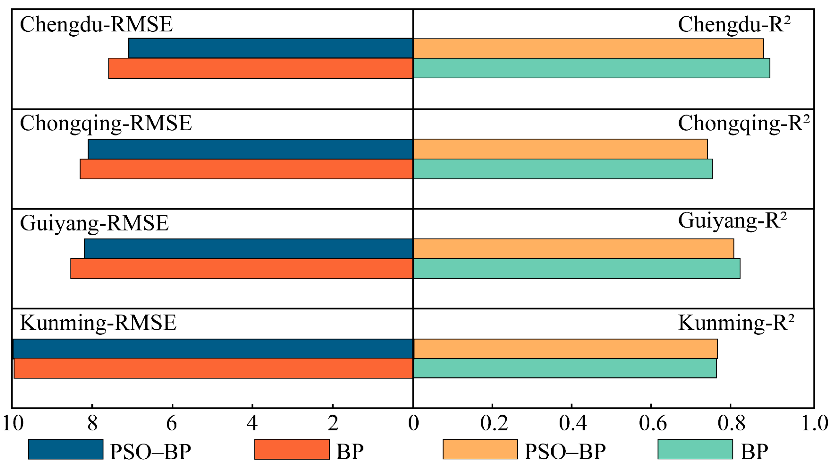
Besides, based on the trained model (1), four subsets of pixels within four cities (Chengdu, Chongqing, Kunming and Guiyang) were selected for validations between the simulated DMSP-OLS NTL data and the correction NTL data of DMSP-OLS in 2013. The accuracy in these cities is acceptable and has a consistent performance (Figure 5). Chengdu has the highest accuracy (R2 = 0.889), followed by the Guiyang (R2 = 0.816). The accuracy rate of other counties is higher than 0.7. Particularly, the RMSE of each city is smaller than 10, and this further indicates the integration model proposed in this study has a high reliability on transforming NPP-VIIRS data to DMSP-OLS-like data.
4.1.2. Results of the Integrated NTL Data
Figure 6 shows the profiles of NTL data of the four cities in 2013. There is an obvious trend that the NTL intensity is higher in the central areas of the city and gradually decreases in the direction away from city centers. By comparing the profiles of original DMSP-OLS data and NPP-VIIRS data with the identical resolution, it can be found that there is a significant difference between them. For DMSP-OLS data, the change of DN is smooth but limited by the saturation effect (peak value of 63), while the DN fluctuations of the original NPP-VIIRS data are accompanied by many dramatic increases and decreases, and have a broader range of values without saturation effect.
Simultaneously, compared to the original DMSP-OLS data, the profiles of the corrected DMSP-OLS data improve significantly in the area of saturation, while the DN amplitude and trend are nearly consistent with the original data in the other area (Figure 6). More importantly, the profiles of the simulated DMSP-OLS data are more consistent with the corrected DMSP-OLS data, which can be presented as two aspects. First, the profiles of simulated DMSP-OLS are smoother than the original NPP-VIIRS profiles, the drastic fluctuations of DN values in urban areas are also restrained. Second, the brightness level of the simulated DMSP-OLS profile is stretched, and the brightness difference between the urban area and the surrounding area is significantly expanded. Although the simulated DMSP-OLS and DMSP-OLS profiles do not exactly match, the brightness ranges and distribution patterns of simulated DMSP-OLS are more consistent with DMSP-OLS than the NPP-VIIRS data. In general, the simulated DMSP-OLS profiles are similar to DMSP-OLS, which also indicates that the proposed method can reliably match DMSP-OLS NTL data with NPP-VIIRS. Therefore, the simulated DMSP-OLS data from 2014 to 2018 are obtained by applying the trained model (1) of 2013 on NPP-VIIRS data.
Figure 7 shows the total nighttime light (TNL) results in time series across study area. The original DMSP-OLS NTL data (2000–2013) are composed by images from multiple sensors, which are short of on-board calibration, therefore there are serious fluctuations in TNL and the problems of discontinuity and incomparability existing in time series (Figure S2). Consequently, the calibrations were applied to DMSP-OLS data firstly, and the continuity and comparability of DMSP-OLS data were significantly improved. Subsequently, the annual NPP-VIIRS data from 2013 to 2019 were correlated with DMSP-OLS data and converted to DMSP-OLS-like data. The results indicate that the time-series of NTL dataset have a high degree of continuity and have a growing trend from 2000 to 2019 (Figure 7). Compared with the GDP from 2000 to 2019, the correlation coefficient between them reached 0.99, therefore the trends in TNL shows a great agreement with economic development, which is consistent with the conclusion of previous studies [43].
Generally, it is reliable to establish a consistent time-series of NTL dataset from 2000 to 2019 by converting the NPP-VIIRS data (2013–2019) to simulate DMSP-OLS data based on the proposed PSO-BP method. Meanwhile, the long-term NTL dataset generated also provide a basis for further evaluating regional poverty.
4.2. Results of Poverty Evaluation
4.2.1. ACPI of the Sample Counties
ACPI values for 38 sample counties of Chongqing in 2019 are shown in Figure 8, which were grouped into five classes based on the natural discontinuous classification. Most of the counties with higher ACPI were concentrated in the major districts in western Chongqing (such as Yuzhong, Jiangbei, Jiulongpo et al.), which have a good social economic basis and development environment, and therefore they are the economic and cultural center of Chongqing. The counties with lower ACPI are widespread across northeastern and southeastern Chongqing with an economy mainly based on agriculture, which is generally consistent with the studies of Yu et al. [8] and Shi et al. [3]. The difference is that the ranks of some counties have changed, and it can be attributed to the work of poverty alleviation. For example, some national poverty counties such as Wulong, Xiushan and Pengshui were considered that they had shacked off poverty in 2019.
Moreover, a histogram shows the county-level CPI in Chongqing from 2000–2019 (Figure 9). ACPI values of all counties in Chongqing in 2019 have significantly improved from 2000, indicating that they have been greatly developed in the past 20 years. According to the list of national poverty counties from China’s National Administration for Rural Revitalization, there were 14 national poverty counties are located in Chongqing. The proportion of national poverty counties in the 14 counties at the bottom of the ACPI ranking in 2000, 2005, 2010 and 2015 reached 85.7%, 78.5%, 78.5% and 78.5% respectively. These results suggest that ACPI can be accurately poverty evaluated.
Above all, the ACPI index proposed in this study is defined by comprehensive evaluation method, and contains several dimensions related to economy, society and nature. It is considered that ACPI can comprehensively and reliably reflect the real development level of counties.
4.2.2. Poverty Evaluation Model Based on NTL Data
Based on the PSO-BP algorithm, a poverty evaluation model was established and ECPI values were obtained. The results are shown in Figure 10a. The results presented a satisfying fitting effect, and the ECPI values matched the ACPI values quite well, which indicated a high effectiveness of the algorithm. Moreover, the R2 (0.959) was higher than the previous research of Yu et al. [8] (0.8554), and Li et al. (0.88) [38]. Their estimated results are based on traditional regression analysis.
The RE values of the ECPI from 2000 to 2019 in sample areas are shown in Figure 10b. The MRE of the 20 years in sample areas was 10.13%, while the maximum and minimum values of RE generated by the model were 15.61% (2000) and 6.81% (2019), respectively. Notably, the mean RE value of ECPI from 2000 to 2012 (11.4%) was higher than subsequent years (7.8%), which might be due to the rough spatial resolution of the DMSP-OLS data and the narrow range of radiation detection. Although the proposed method improved the usability of DMSP-OLS data in this study, many details might have been left out in the data production procedure. However, compared to the 11.20% of MRE in the work of Pan and Hu [44], our results indicated that the poverty evaluation model proposed in this study was feasible and reliable.
4.3. Spatiotemporal Dynamics of Poverty
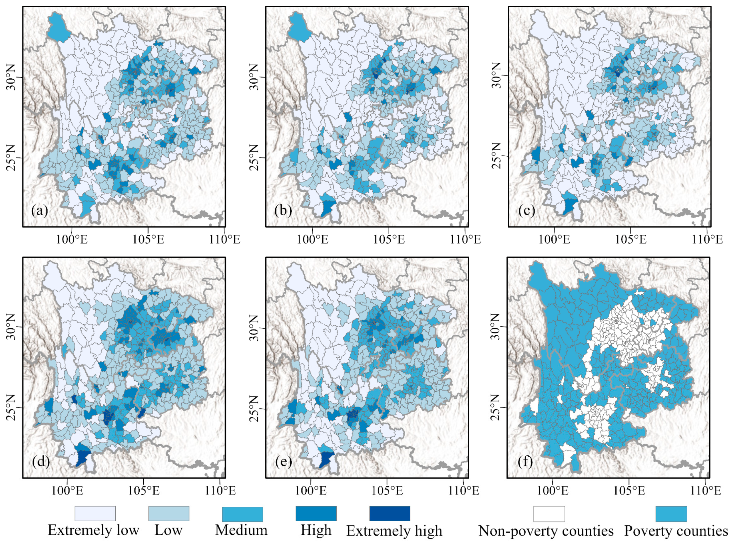
Figure 11 shows the spatial pattern of county-level ECPI in southwestern China from 2000 to 2019. To better reflect the spatial patterns of poverty, the ECPI values of the 435 counties were divided into five classes according to natural breaks: extremely low, low, medium, high and extremely high. As we can see, there are obvious dynamic characteristics with ECPI that change over time and regional characteristics with spatial distribution. First, the low values of ECPI were contiguously distributed in northwest Sichuan, northwest Yunnan and Yunnan-Guizhou plateau, where they were usually accompanied by unfavorable natural environment and traffic conditions. Geographical barriers are a key factor blocking local development and causing poverty, and the region with high elevation and dramatic mountain terrain usually has a high occurrence of poverty. Moreover, the high values of ECPI were mainly concentrated on the relatively flat urban agglomerations, such as Chengdu Plain, central Yunnan, central Chongqing and central Guizhou, which had fertile land, convenient transportation and solid foundation. Therefore, development opportunities can be more easily gained in those regions, and thus get rid of poverty for people. Moreover, the development level of counties that are adjacent to counties with high CPI values have risen faster than other areas, and it is easier to get rid of poverty, which is matched by the regional development policy and practical conditions.
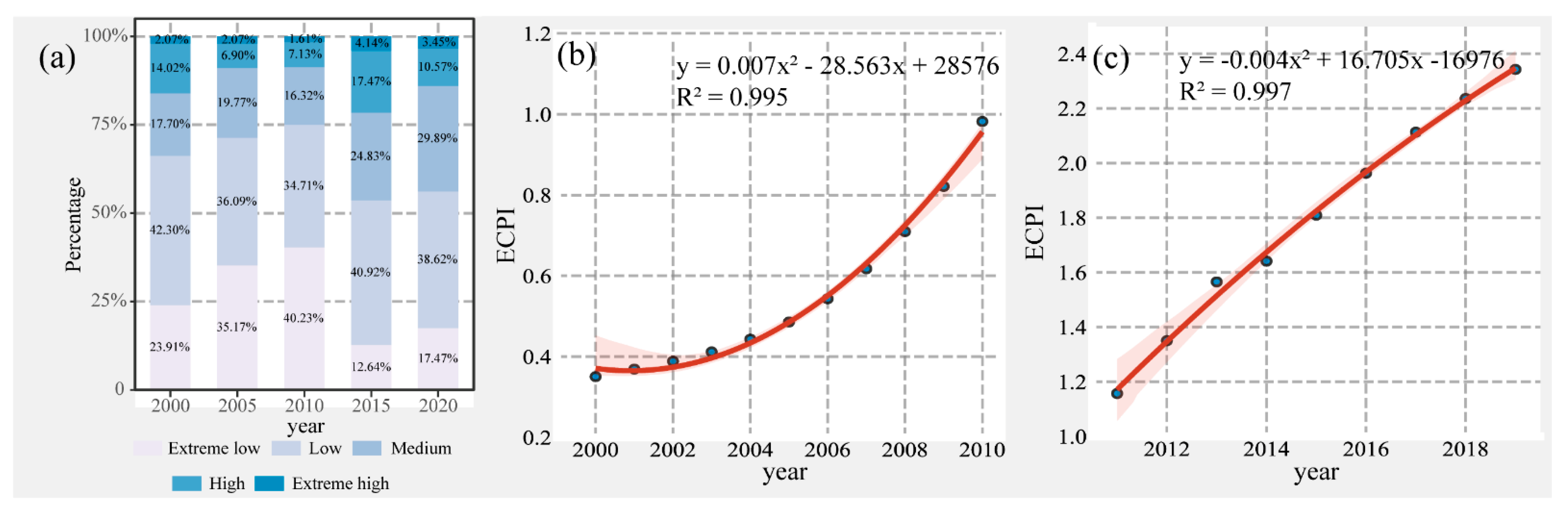
From 2000 to 2019, the proportion of counties with extremely high and high ECPI is between 8.74% and 16.09%, while the proportion of others is between 83.91% and 91.26% (Figure 12a), which also indicates that the situation of multidimensional poverty in southwestern China is seriously unbalanced. However, with socio-economic development, the proportion of extremely low and low decreased, while that of medium increased. Significantly, Figure 12b,c indicated that ECPI of southwestern China also showed an upward trend from 2000 to 2019, indicating that under the development of poverty alleviation and development work, regional development has received better support, and the overall situation of multidimensional poverty has been greatly improved. It is noticed that the ECPI illustrated an accelerated trend before 2011, but slowed down from 2011 to 2019. During the period of 2000 to 2010, the intensity of efforts to alleviate poverty and investments has increased significantly, resulting in a significant reduction in the poverty-stricken population, and people have generally solved the problem of food and clothing. After the previous period (2000–2010) of poverty alleviation, the spatial patterns of poverty have changed significantly, and the remaining poverty-stricken population tend to be dispersed, and mainly concentrated in areas with harsh natural environment and inconvenient transportation. Meanwhile, the government implemented the policy of “precise poverty alleviation” during this period of 2011 to 2019, targeting poverty alleviation to households and individuals, the cost of poverty alleviation has risen, making it more difficult for poverty alleviation. Therefore, the ECPI of the period has slowed down compared with the previous period.
4.4. Uncertainties in the Results
This study proposes a useful method to integrate DMSP and VIIRS data to evaluate poverty in southwest China. However, it is worth mentioning that there are still some limitations in this study. First, the spatial distribution of high DN values in the simulated DMSP-OLS data is smaller than that of the original DMSP-OLS data (Figure 6). Then, the method of this study cannot completely eliminate the defects in the DMSP-OLS data, such as light saturation in urban regions with high light intensity [25]. Moreover, the overpass time of DMSP-OLS data is evening (19:30), while the overpass time of NPP-VIIRS data is after-midnight (01:30). The difference of overpass time may have some effect on the detection of lights [29]. These shortcomings present a challenge to integrate the DMSP-OLS data and NPP-VIIRS data for generating consistent NTL data. Next, we estimated county-level poverty with nighttime light data. The model coefficients are kept constant for all pixels in a county, but the light data depend on the city of the county, which implies that ECPI only reveals the overall development of a county, while the bias in low-DN areas is ignored.
5. Conclusions
This study introduced NTL data as a proxy to measure the poverty conditions of each county in southwest China. Due to both DMSP-OLS and NPP-VIIRS NTL data having defects, this study combined the PSO-BP algorithm to investigate the relationship between the DMSP-OLS data and NPP-VIIRS data. Then, we integrated two datasets at the pixel level, and established a consistent time-series of NTL dataset during the period of 2000–2019. The results displayed that the application of supplementary input parameters and PSO-BP algorithm was advantageous for constructing the matching relationship between DMSP-OLS and NPP-VIIRS data (R2 = 0.84). After calibration, the continuity and comparability of DMSP-OLS data were significantly improved. Subsequently, the annual NPP-VIIRS data (2013–2019) related to DMSP-OLS data and converted to DMSP-OLS-like data. The trend in TNL showed a great agreement with economic development (r = 0.99). Next, ACPI was employed as an indicator of county-level multidimensional poverty based on 11 socioeconomic and natural variables, and which could be the reference for the poverty evaluation using NTL data. The poverty evaluation model was established by exploring the relationship between ACPI and NTL feature variables in southwest China. Third, the RMSE between ACPI based on statistical data and ECPI based on NTL data was approximately 0.19 (R2 = 0.96), which was higher than the previous research. According to the ECPI, this study found that ECPI illustrated an accelerated trend before 2011, but slowed down from 2011 to 2019. Geographical barriers (high elevation and dramatic mountain terrain) are also a key factor that cause poverty. However, the high values of ECPI were mainly concentrated on the relatively flat urban agglomerations. Based on the integrated NTL data, a poverty evaluation model is proposed in this study, which has wide applicability and effectiveness. This model can be used as a reference for future socio-economic development studies to monitor poverty and socio-economic changes at different regional scales.
Supplementary Materials
The following supporting information can be downloaded at: https://www.mdpi.com/article/10.3390/rs14030600/s1, Figure S1. The population (a) and GDP (b) of the southwestern China in 2019. Figure S2. The original NTL data from 2000 to 2013 are composed by images from multiple sensors. Table S1. List of PSO-BP algorithm parameter settings. Table S2. Abbreviation in this paper and its description.
Author Contributions
Conceptualization, K.L. and J.X.; methodology, Z.Y., Z.W. and K.L.; software, Z.Y. and Z.W.; validation, Z.Y. and H.S.; formal analysis, Z.Y. and Z.W.; investigation, Z.Y. and W.C.; resources, K.L.; data curation, C.Y., and Z.Y.; writing-original draft preparation, Z.Y.; writing-review and editing, Z.W.; visualization, Z.Y.; supervision, Z.W.; project administration, Z.Y.; funding acquisition, J.X. All authors have read and agreed to the published version of the manuscript.
Funding
This research was funded by the Key R&D project of Sichuan Science and Technology Department(Grant No. 2021YFQ0042), National Key R&D Program of China (2020YFD1100701), Strategic Priority Research Program of the Chinese Academy of Sciences (Grant No. XDA20030302), Science and Technology Project of Xizang Autonomous Region (Grant No. XZ201901-GA-07), National Flash Flood Investigation and Evaluation Project (Grant No. SHZH-IWHR-57), and Project form Science and Technology Bureau of Altay Region in Yili Kazak Autonomous Prefecture(Grant No. Y99M4600AL).
Data Availability Statement
The data used to support the findings of this study are included within the article.
Conflicts of Interest
The authors declare no conflict of interest.
References
- Steele, J.E.; Sundsøy, P.R.; Pezzulo, C.; Alegana, V.A.; Bird, T.J.; Blumenstock, J.; Bjelland, J.; Engø-Monsen, K.; Montjoye, Y.-A.d.; Iqbal, A.M.; et al. Mapping poverty using mobile phone and satellite data. J. R. Soc. Interface 2017, 14, 20160690. [Google Scholar] [CrossRef] [PubMed]
- Niu, T.; Chen, Y.; Yuan, Y. Measuring urban poverty using multi-source data and a random forest algorithm: A case study in Guangzhou. Sustain. Cities Soc. 2020, 54, 102014. [Google Scholar] [CrossRef]
- Shi, K.; Chang, Z.; Chen, Z.; Wu, J.; Yu, B. Identifying and evaluating poverty using multisource remote sensing and point of interest (POI) data: A case study of Chongqing, China. J. Clean. Prod. 2020, 255, 120245. [Google Scholar] [CrossRef]
- Haushofer, J.; Fehr, E. On the psychology of poverty. Sci. Total Environ. 2014, 344, 862–867. [Google Scholar] [CrossRef] [PubMed]
- Ren, Q.; Huang, Q.; He, C.; Tu, M.; Liang, X. The poverty dynamics in rural China during 2000–2014: A multi-scale analysis based on the poverty gap index. J. Geogr. Sci. 2018, 28, 1427–1443. [Google Scholar] [CrossRef] [Green Version]
- Kubiszewski, I.; Costanza, R.; Franco, C.; Lawn, P.; Talberth, J.; Jackson, T.; Aylmer, C. Beyond GDP: Measuring and achieving global genuine progress. Ecol. Econ. 2013, 93, 57–68. [Google Scholar] [CrossRef] [Green Version]
- Bossert, W.; Chakravarty, S.R.; D’Ambrosio, C. Multidimensional Poverty and Material Deprivation with Discrete Data. Rev. Income Wealth 2013, 59, 29–43. [Google Scholar] [CrossRef] [Green Version]
- Yu, B.; Shi, K.; Hu, Y.; Huang, C.; Chen, Z.; Wu, J. Poverty Evaluation Using NPP-VIIRS Nighttime Light Composite Data at the County Level in China. IEEE J. Sel. Top. Appl. Earth Obs. Remote Sens. 2017, 8, 1217–1229. [Google Scholar] [CrossRef]
- Wang, Y.; Wang, B. Multidimensional poverty measure and analysis: A case study from Hechi City, China. SpringerPlus 2016, 5, 642. [Google Scholar] [CrossRef] [Green Version]
- Zhao, X.; Yu, B.; Liu, Y.; Chen, Z.; Li, Q.; Wang, C.; Wu, J. Estimation of Poverty Using Random Forest Regression with Multi-Source Data: A Case Study in Bangladesh. Remote Sens. 2019, 11, 375. [Google Scholar] [CrossRef] [Green Version]
- Burke, M.; Driscoll, A.; Lobell, D.B.; Ermon, S. Using satellite imagery to understand and promote sustainable development. Science 2021, 371, eabe8628. [Google Scholar] [CrossRef] [PubMed]
- Zhao, M.; Zhou, Y.; Li, X.; Cao, W.; He, C.; Yu, B.; Li, X.; Elvidge, C.D.; Cheng, W.; Zhou, C. Applications of Satellite Remote Sensing of Nighttime Light Observations: Advances, Challenges, and Perspectives. Remote Sens. 2019, 11, 1971. [Google Scholar] [CrossRef] [Green Version]
- Bennett, M.M.; Smith, L.C. Advances in using multitemporal night-time lights satellite imagery to detect, estimate, and monitor socioeconomic dynamics. Remote Sens. Environ. 2017, 192, 176–197. [Google Scholar] [CrossRef]
- Chen, Z.; Yu, B.; Zhou, Y.; Liu, H.; Yang, C.; Shi, K.; Wu, J. Mapping Global Urban Areas from 2000 to 2012 Using Time-Series Nighttime Light Data and MODIS Products. IEEE J. Sel. Top. Appl. Earth Obs. Remote Sens. 2019, 12, 1143–1153. [Google Scholar] [CrossRef]
- Wang, L.; Wang, S.; Zhou, Y.; Liu, W.; Hou, Y.; Zhu, J.; Wang, F. Mapping population density in China between 1990 and 2010 using remote sensing. Remote Sens. Environ. 2018, 210, 269–281. [Google Scholar] [CrossRef]
- Zhao, M.; Cheng, W.; Zhou, C.; Li, M.; Wang, N.; Liu, Q. GDP Spatialization and Economic Differences in South China Based on NPP-VIIRS Nighttime Light Imagery. Remote Sens. 2017, 9, 673. [Google Scholar] [CrossRef] [Green Version]
- Xie, Y.; Weng, Q. Detecting urban-scale dynamics of electricity consumption at Chinese cities using time-series DMSP-OLS (Defense Meteorological Satellite Program-Operational Linescan System) nighttime light imageries. Energy 2016, 100, 177–189. [Google Scholar] [CrossRef]
- Elvidge, C.D.; Sutton, P.C.; Ghosh, T.; Tuttle, B.T.; Baugh, K.E.; Bhaduri, B.; Bright, E. A global poverty map derived from satellite data. Comput. Geosci. 2009, 35, 1652–1660. [Google Scholar] [CrossRef]
- Li, G.; Cai, Z.; Liu, X.; Liu, J.; Su, S. A comparison of machine learning approaches for identifying high-poverty counties: Robust features of DMSP/OLS night-time light imagery. Int. J. Remote Sens. 2019, 40, 5716–5736. [Google Scholar] [CrossRef]
- Zhao, M.; Zhou, Y.; Li, X.; Cheng, W.; Zhou, C.; Ma, T.; Li, M.; Huang, K. Mapping urban dynamics (1992–2018) in Southeast Asia using consistent nighttime light data from DMSP and VIIRS. Remote Sens. Environ. 2020, 248, 111980. [Google Scholar] [CrossRef]
- Zhu, X.; Ma, M.; Yang, H.; Ge, W. Modeling the Spatiotemporal Dynamics of Gross Domestic Product in China Using Extended Temporal Coverage Nighttime Light Data. Remote Sens. 2017, 9, 626. [Google Scholar] [CrossRef] [Green Version]
- Zhao, J.; Ji, G.; Yue, Y.; Lai, Z.; Chen, Y.; Yang, D.; Yang, X.; Wang, Z. Spatio-temporal dynamics of urban residential CO2 emissions and their driving forces in China using the integrated two nighttime light datasets. Appl. Energy 2019, 235, 612–624. [Google Scholar] [CrossRef]
- Shao, X.; Cao, C.; Zhang, B.; Qiu, S.; Elvidge, C.; Von Hendy, M. Radiometric calibration of DMSP-OLS sensor using VIIRS day/night band. In Proceedings of the Earth Observing Missions and Sensors: Development, Implementation, and Characterization III, Beijing, China, 3–15 October 2014; p. 92640A. [Google Scholar]
- Li, X.; Li, D.; Xu, H.; Wu, C. Intercalibration between DMSP/OLS and VIIRS night-time light images to evaluate city light dynamics of Syria’s major human settlement during Syrian Civil War. Int. J. Remote Sens. 2017, 38, 5934–5951. [Google Scholar] [CrossRef]
- Lu, D.; Wang, Y.; Yang, Q.; Su, K.; Zhang, H.; Li, Y. Modeling Spatiotemporal Population Changes by Integrating DMSP-OLS and NPP-VIIRS Nighttime Light Data in Chongqing, China. Remote Sens. 2021, 13, 284. [Google Scholar] [CrossRef]
- Li, X.; Zhou, Y.; Zhao, M.; Zhao, X. A harmonized global nighttime light dataset 1992–2018. Sci. Data 2020, 7, 168. [Google Scholar] [CrossRef]
- Gori, M.; Tesi, A. On the problem of local minima in backpropagation. IEEE Trans. Pattern Anal. Mach. Intell. 1992, 14, 76–86. [Google Scholar] [CrossRef] [Green Version]
- Zhang, J.-R.; Zhang, J.; Lok, T.-M.; Lyu, M.R. A hybrid particle swarm optimization-back-propagation algorithm for feedforward neural network training. Appl. Math. Comput. 2007, 185, 1026–1037. [Google Scholar] [CrossRef]
- Zhao, M.; Zhou, Y.; Li, X.; Zhou, C.; Cheng, W.; Li, M.; Huang, K. Building a Series of Consistent Night-Time Light Data (1992–2018) in Southeast Asia by Integrating DMSP-OLS and NPP-VIIRS. IEEE Trans. Geosci. Remote Sens. 2020, 58, 1843–1856. [Google Scholar] [CrossRef]
- Lv, Q.; Liu, H.; Wang, J.; Liu, H.; Shang, Y. Multiscale analysis on spatiotemporal dynamics of energy consumption CO2 emissions in China: Utilizing the integrated of DMSP-OLS and NPP-VIIRS nighttime light datasets. Sci. Total Environ. 2020, 703, 134394. [Google Scholar] [CrossRef]
- Sun, Y.; Zheng, S.; Wu, Y.; Schlink, U.; Singh, R.P. Spatiotemporal Variations of City-Level Carbon Emissions in China during 2000–2017 Using Nighttime Light Data. Remote Sens. 2020, 12, 2916. [Google Scholar] [CrossRef]
- Chen, J.; Gao, M.; Cheng, S.; Hou, W.; Song, M.; Liu, X.; Liu, Y.; Shan, Y. County-level CO2 emissions and sequestration in China during 1997–2017. Sci. Data 2020, 7, 391. [Google Scholar] [CrossRef] [PubMed]
- Chen, M.; Cai, H.; Yang, X.; Jin, C. A novel classification regression method for gridded electric power consumption estimation in China. Sci. Rep. 2020, 10, 18558. [Google Scholar] [CrossRef] [PubMed]
- Ma, J.; Guo, J.; Ahmad, S.; Li, Z.; Hong, J. Constructing a New Inter-Calibration Method for DMSP-OLS and NPP-VIIRS Nighttime Light. Remote Sens. 2020, 12, 937. [Google Scholar] [CrossRef] [Green Version]
- Jeswani, R.; Kulshrestha, A.; Gupta, P.K.; Srivastav, S. Evaluation of the consistency of DMSP-OLS and SNPP-VIIRS Night-time Light Datasets. J. Geomat. 2019, 13, 98–105. [Google Scholar]
- Mohamad, E.T.; Armaghani, D.J.; Momeni, E.; Yazdavar, A.H.; Ebrahimi, M. Rock strength estimation: A PSO-based BP approach. Neural Comput. Appl. 2018, 30, 1635–1646. [Google Scholar] [CrossRef]
- Shi, Y.; Eberhart, R.C. Parameter selection in particle swarm optimization. In Proceedings of the Evolutionary Programming VII, San Diego, CA, USA, 25–27 March 1998; pp. 591–600. [Google Scholar]
- Li, C.; Yang, W.; Tang, Q.; Tang, X.; Lei, J.; Wu, M.; Qiu, S. Detection of Multidimensional Poverty Using Luojia 1-01 Nighttime Light Imagery. J. Indian Soc. Remote Sens. 2020, 48, 963–977. [Google Scholar] [CrossRef]
- DFID. DFID Sustainable Livelihoods Guidance Sheets. 1999. Available online: www.ennonline.net/dfidsustainableliving (accessed on 5 May 2021).
- Yin, J.; Qiu, Y.; Zhang, B. Identification of Poverty Areas by Remote Sensing and Machine Learning: A Case Study in Guizhou, Southwest China. ISPRS Int. J. Geo-Inf. 2021, 10, 11. [Google Scholar] [CrossRef]
- Wang, W.; Cheng, H.; Zhang, L. Poverty assessment using DMSP/OLS night-time light satellite imagery at a provincial scale in China. Adv. Space Res. 2012, 49, 1253–1264. [Google Scholar] [CrossRef]
- Fang, D.; Ma, W. Study on the Measurement of China’s Intter-Provincial High-Quality Development and Its Spatial-Temporal Characteristics. Reg. Econ. Rev. 2019, 2, 61–70. [Google Scholar]
- Zhao, N.; Liu, Y.; Cao, G.; Samson, E.L.; Zhang, J. Forecasting China’s GDP at the pixel level using nighttime lights time series and population images. GIScience Remote Sens. 2017, 54, 407–425. [Google Scholar] [CrossRef]
- Pan, J.; Hu, Y. Spatial Identification of Multi-dimensional Poverty in Rural China: A Perspective of Nighttime-Light Remote Sensing Data. J. Indian Soc. Remote Sens. 2018, 46, 1093–1111. [Google Scholar] [CrossRef]
Figure 1.
The location of the study area.

Figure 2.
The workflow of the methodology application in this study. (a) denote the temporal trends of ECPI in the southwest regions from 2000 to 2010, and (b) 2011 to 2019.
Figure 2.
The workflow of the methodology application in this study. (a) denote the temporal trends of ECPI in the southwest regions from 2000 to 2010, and (b) 2011 to 2019.

Figure 3.
Distribution of the inter-calibration samples in southwestern China.

Figure 4.
Scatter density plots of four trained models in Southwest China in 2013. The value at x-axis denoted the DN value of four ANNs models, and the value at y-axis denoted the DN value of desired output.
Figure 4.
Scatter density plots of four trained models in Southwest China in 2013. The value at x-axis denoted the DN value of four ANNs models, and the value at y-axis denoted the DN value of desired output.

Figure 5.
The validation statistical indices (RMSE: root mean square error, and R2: determination coefficient) between the simulated DMSP-OLS NTL data and DMSP-OLS correction NTL data of 2013 in four cities.
Figure 5.
The validation statistical indices (RMSE: root mean square error, and R2: determination coefficient) between the simulated DMSP-OLS NTL data and DMSP-OLS correction NTL data of 2013 in four cities.

Figure 6.
Google Earth’s image of Chengdu (a), Guiyang (b), Kunming (c), Chongqing (d) region and their surrounding areas, and NTL profile of four nighttime light data (original DMSP-OLS, original NPP-VIIRS, corrected DMSP-OLS, and simulated DMSP-OLS) in 2013.
Figure 6.
Google Earth’s image of Chengdu (a), Guiyang (b), Kunming (c), Chongqing (d) region and their surrounding areas, and NTL profile of four nighttime light data (original DMSP-OLS, original NPP-VIIRS, corrected DMSP-OLS, and simulated DMSP-OLS) in 2013.

Figure 7.
Time series and correlation of the integrated NTL data and GDP from 2000 to 2019 across southwestern China.
Figure 7.
Time series and correlation of the integrated NTL data and GDP from 2000 to 2019 across southwestern China.

Figure 8.
Spatial distribution of ACPI classification of Chongqing in 2019.

Figure 9.
The histogram of county-level ACPI values of Chongqing in 2000, 2005, 2010, 2015 and 2019.
Figure 9.
The histogram of county-level ACPI values of Chongqing in 2000, 2005, 2010, 2015 and 2019.

Figure 10.
(a) Estimated CPI values and ACPI values in the sample areas. The red line indicated the linear fitting line, and the light red areas correspond to 95% confidence intervals. (b) RE of the estimated CPI from 2000 to 2019 in sample areas. The blue bar indicated the RE value during the period of 2000–2012, and the orange bar indicated the RE value during the period of 2013–2019.

Figure 11.
Spatial patterns of ECPI at the county level in 2000 (a), 2005 (b), 2010 (c), 2015 (d), 2019 (e), and the distribution of national-level poverty county (f).
Figure 11.
Spatial patterns of ECPI at the county level in 2000 (a), 2005 (b), 2010 (c), 2015 (d), 2019 (e), and the distribution of national-level poverty county (f).

Figure 12.
Percentage of counties at different levels of ECPI in Southwestern China (a). Variation trends of ECPI of the southwest regions from 2000 to 2010 (b) and 2011 to 2019 (c).
Figure 12.
Percentage of counties at different levels of ECPI in Southwestern China (a). Variation trends of ECPI of the southwest regions from 2000 to 2010 (b) and 2011 to 2019 (c).


Table 1.
Description of each data sources used in this study.
| Data | Data Description | Year | Source |
|---|---|---|---|
| DMSP-OLS | Version 4 DMSP-OLS annual stable NTL data | 2000–2013 | https://eogdata.mines.edu/products/dmsp/, accessed on 20 April 2021 |
| NPP-VIIRS | Vision 1 NPP-VIIRS monthly vcm NTL data | 2012–2019 | https://eogdata.mines.edu/products/vnl/, accessed on 22 April 2021 |
| Boundaries | Shapefiles of county-level regions in Sichuan, Chongqing, Yunnan and Guizhou | 2015 | Resources and Environmental Science and Data Center (https://www.resdc.cn/), accessed on 23 April 2021 |
| statistical data | Socioeconomic statistical data of county-level regions in Sichuan, Chongqing, Yunnan and Guizhou | 2000–2019 | Statistical Yearbooks of Sichuan, Chongqing, Yunnan, Guizhou and other corresponding counties, accessed on 5 April 2021 |
| DEM | SRTMDEM 90 m raster | - | Geospatial Data Cloud (http://www.gscloud.cn/), accessed on 23 April 2021 |
Table 2.
Basic descriptions of ANNs trained in this study.
| Model | Input Parameters | Output Parameters | Training Algorithm |
|---|---|---|---|
| 1 | Log_V, X, Y, Area | DMSP-OLS | PSO-BP |
| 2 | Log_V | DMSP-OLS | PSO-BP |
| 3 | Log_V, X, Y, Area | DMSP-OLS | BP |
| 4 | Log_V | DMSP-OLS | BP |
Table 3.
Evaluation indices and weight distribution of multidimensional poverty.
| ID | Index | Attribute | Weight |
|---|---|---|---|
| 1 | Per capita GDP | + | 0.1308 |
| 2 | Per capita net income of rural population | + | 0.0818 |
| 3 | Per capita fiscal revenue | + | 0.1532 |
| 4 | Per capita health care institutions | + | 0.0941 |
| 5 | Beds in health per 1000 | + | 0.0868 |
| 6 | Per capita total investment in fixed assets | + | 0.1319 |
| 7 | Per capita total retail sales of consumer goods | + | 0.1779 |
| 8 | Proportion of primary school students | + | 0.0515 |
| 9 | Proportion of secondary school students | + | 0.0337 |
| 10 | Proportion of slope area above 15° | − | 0.0360 |
| 11 | Average altitude | − | 0.0216 |
Note: “+” denotes the positive attribution, “−” denotes the negative attribution.
Table 4.
Detail description of feature variables.
| Abbreviation | Detail Description |
|---|---|
| F1 | Average of all pixels of the NTL imagery within the county’s boundary |
| F2 | Average light index of all pixels within the county’s boundary |
| F3 | Variance of all pixels within the county’s boundary |
| F4 | Standard deviation of all pixels within the county’s boundary |
| F5 | Sum of squares of deviation of all pixels within the county’s boundary |
| F6 | Total value of all pixels within the county’s boundary |
| F7 | Number of pixels within the county’s boundary |
| F8 | Number of pixels greater than zero within the county’s boundary |
| F9 | Largest value of all pixels within the county’s boundary |
| F10 | Smallest value of all pixels within the county’s boundary |
| F11 | Range between the largest and smallest value of all pixels within the county’s boundary |
| F12 | Local autocorrelation Moran’s I of the counties |
Table 5.
Correlation analysis between CPI and NTL feature variables.
| Abbreviation | Correlation Coefficient | Abbreviation | Correlation Coefficient |
|---|---|---|---|
| F1 | 0.550 ** | F7 | −0.373 ** |
| F2 | 0.594 ** | F8 | 0.340 ** |
| F3 | 0.307 ** | F9 | 0.534 ** |
| F4 | 0.409 ** | F10 | 0.371 ** |
| F5 | 0.372 ** | F11 | 0.267 ** |
| F6 | 0.604 ** | F12 | 0.129 ** |
Note: ** is significantly different from zero at the 1% level.
Table 6.
Fitting results of five regression models.
| Model Type | Expression | R2 | Significance |
|---|---|---|---|
| Linear | Y = 19.569 ∗ x + 1.407 | 0.824 | <0.01 |
| Quadratic polynomial | Y = 15.199 ∗ x2 + 1.384∗x + 0.005 | 0.827 | <0.01 |
| Log function | Y = 14.934 ∗ ln(x) + 27.275 | 0.607 | <0.01 |
| Power function | Y = x0.742 + 18.561 | 0.7 | <0.01 |
| Exponential | Y = 0.845x + 5.615 | 0.718 | <0.01 |
Publisher’s Note: MDPI stays neutral with regard to jurisdictional claims in published maps and institutional affiliations. |
© 2022 by the authors. Licensee MDPI, Basel, Switzerland. This article is an open access article distributed under the terms and conditions of the Creative Commons Attribution (CC BY) license (https://creativecommons.org/licenses/by/4.0/).
Share and Cite
MDPI and ACS Style
Yong, Z.; Li, K.; Xiong, J.; Cheng, W.; Wang, Z.; Sun, H.; Ye, C. Integrating DMSP-OLS and NPP-VIIRS Nighttime Light Data to Evaluate Poverty in Southwestern China. Remote Sens. 2022, 14, 600. https://doi.org/10.3390/rs14030600
AMA Style
Yong Z, Li K, Xiong J, Cheng W, Wang Z, Sun H, Ye C. Integrating DMSP-OLS and NPP-VIIRS Nighttime Light Data to Evaluate Poverty in Southwestern China. Remote Sensing. 2022; 14(3):600. https://doi.org/10.3390/rs14030600
Chicago/Turabian StyleYong, Zhiwei, Kun Li, Junnan Xiong, Weiming Cheng, Zegen Wang, Huaizhang Sun, and Chongchong Ye. 2022. "Integrating DMSP-OLS and NPP-VIIRS Nighttime Light Data to Evaluate Poverty in Southwestern China" Remote Sensing 14, no. 3: 600. https://doi.org/10.3390/rs14030600
Note that from the first issue of 2016, this journal uses article numbers instead of page numbers. See further details here.