
Flash Flood Water Depth Estimation Using SAR Images, Digital Elevation Models, and Machine Learning Algorithms


Civil Engineering Department, College of Engineering, Najran University, King Abdulaziz Road, Najran P.O. Box 1988, Saudi Arabia
Remote Sens. 2022, 14(3), 440; https://doi.org/10.3390/rs14030440
Submission received: 22 December 2021
/
Revised: 7 January 2022
/
Accepted: 10 January 2022
/
Published: 18 January 2022
(This article belongs to the Special Issue Remote Sensing in Urban Flooding Monitoring)
Abstract
:In this article, the local spatial correlation of multiple remote sensing datasets, such as those from Sentinel-1, Sentinel-2, and digital surface models (DSMs), are linked to machine learning (ML) regression algorithms for flash floodwater depth retrieval. Edge detection filters are applied to remote sensing images to extract features that are used as independent features by ML algorithms to estimate flood depths. Data of dependent variables were obtained from the Hydrologic Engineering Center’s River Analysis System (HEC-RAS 2D) simulation model, as applied to the New Cairo, Egypt, post-flash flood event from 24–26 April 2018. Gradient boosting regression (GBR), random forest regression (RFR), linear regression (LR), extreme gradient boosting regression (XGBR), multilayer perceptron neural network regression (MLPR), k-nearest neighbors regression (KNR), and support vector regression (SVR) were used to estimate floodwater depths; their outputs were compared and evaluated for accuracy using the root-mean-square error (RMSE). The RMSE accuracy for all ML algorithms was 0.18–0.22 m for depths less than 1 m (96% of all test data), indicating that ML models are relatively portable and capable of computing floodwater depths using remote sensing data as an input.
Keywords:
floodwater depth; ML; Sentinel-1; SAR data; DEM; remote sensing; hydraulic modeling; feature extraction1. Introduction
Floodwater depth identification during or after flash flood events is critical in determining hazard degrees and risk zone maps for the economy and human life [1,2]. Compared with direct surveying methods, measurement techniques, such as side-scan and multi-beam sonar, hydrologic modeling, and flow water depth, based on remote sensing are fast, large-scale, and quasi-synchronous with high spatial resolutions. Furthermore, direct surveying methods to determine floodwater depth can be extremely precise, but they are greatly influenced by weather conditions and costly, and surveying field crews are not authorized to reach sensitive flooded areas.
In addition, optical and synthetic aperture radar (SAR) images, and the digital elevation model (DEM) based on airborne light detection and ranging (LiDAR), have been integrated and classified for floodwater surface identification [3,4]. Although SAR data are superior to optical satellite data, as SARs can penetrate cloud cover, they suffer from a long revisit time [5,6,7].
Studies have employed a variety of hydrodynamic 1D, 2D, and 3D software to simulate water levels and floodwater depths, including HEC-RAS, Delft-3D, and LISFLOOD-FP [8,9]. These models require rainfall, soil moisture, flood maps, gauge discharge, cross-sections, and other hydrological inputs to simulate water depth. The disadvantage of employing hydrodynamic models to simulate floodwater depth is the requirement of a large input dataset and extensive computation and calibration.
Recently, the growth of urban regions and infrastructures such as highways and trains has extended the flood-prone regions in New Cairo, Egypt, which has increased the severity of floods [10]. Several studies have mapped flood inundation in New Cairo, but none have addressed floodwater depth. Numerous hydrological characteristics and flood models, such as the Hydraulic Engineering Center’s River Analysis System (HEC-RAS), have been applied to map and forecast flood inundation [11,12,13], and machine learning (ML) algorithms have been used to map flood inundation [14,15,16]. No study has attempted to quantify floodwater depth and duration during flood disasters in Egypt so far.
Supervised ML regression algorithms are used to learn a function that combines a set of feature data (independent variables) to predict a dependent variable [17,18]. Random forest regression (RFR) is a kind of ensemble learning [19], i.e., a decision tree supervised ML algorithm based on a set of rules [17].
Furthermore, ML has been used for data extraction, pattern recognition, regression, and classification problems since the start of the 21st century. Research has shown that ML algorithms, such as support vector machine (SVM), RFR, and extreme gradient boosting (XGBR), can efficiently produce spatial predictions [19,20]. RF and XGBR use both decision trees and the bagging technique [21]. Some researchers have trained ML algorithms to estimate water depths using the pixel reflectance values of satellite data, and validated the results through field observation [22].
The current work aims to estimate flash flood water depths by concatenating the spectral information of remote sensing data, such as Sentinel-1 SAR data, digital surface models (DSMs), and land-use maps, at feature levels, and apply a regression algorithm using ML techniques, such as gradient boosting regression (GBR), RFR, linear regression (LR), XGBR, multilayer perceptron neural network regression (MLPR), k-nearest neighbors regression (KNR), and support vector regression (SVR). ML has many properties that make it appropriate for obtaining water depths from remote sensing images. For example, ML algorithms are ideal for processing locally joined data, such as raster data with a spatial grid structure. Moreover, the floodwater levels of unknown locations can be considered the weighted averages of nearby known water depths, as obtained by geographic interpolation. Therefore, I investigate the impact of adjacent pixels of remote sensing data on floodwater depth prediction through ML algorithms. An informative and appropriate number of features should be derived for the subsequent regression ML algorithms. The performance of extracted features and their importance in improving accuracy and accelerating the algorithm are investigated.
2. Study Area and Dataset
2.1. Study Area
New Cairo is in the southeast of Egypt’s Cairo Province. It was established in 2000, with a land area of approximately 70,000 acres. A 90-square-kilometer area with altitudes ranging from 200 m to 420 m above the mean sea level was chosen to model flash floodwater depths. Figure 1 shows a true-color Sentinel-2 image of the study area, from which a land-use map was created for use in calculating roughness values.
2.2. Rainfall Intensity Data
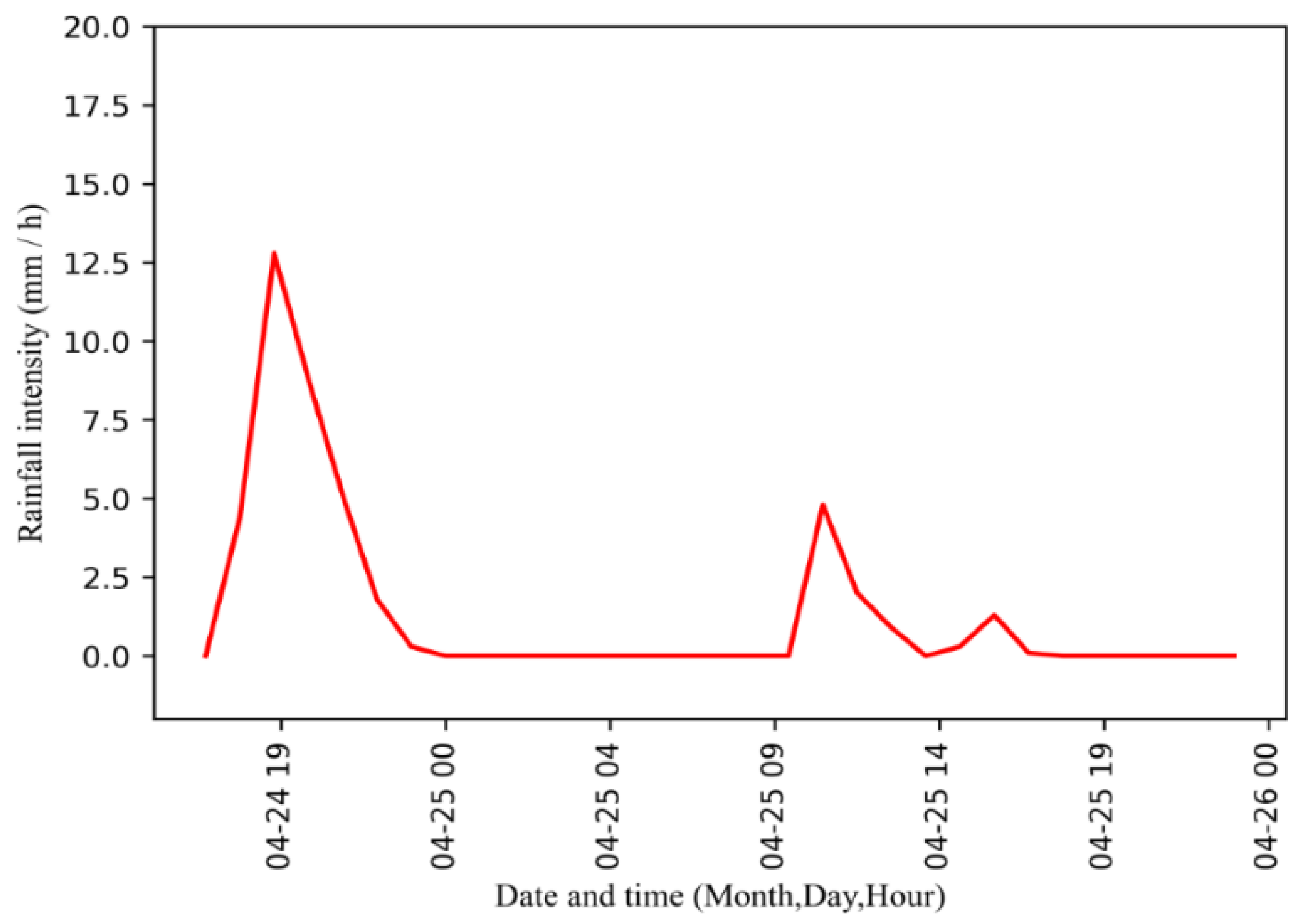
Cairo has a four-season hot desert climate. The study area receives the majority of its rainfall from November through April. Daily rainfall data for the area were obtained from the NASA Prediction of Worldwide Energy Resources (POWER) project, which delivers global weather data with a spatial resolution of 0.5°. Based on historical meteorological information collected from the POWER website for 1981–2018, the average annual precipitation in the watershed is 51.2 mm/y (https://power.larc.nasa.gov/data-access-viewer/ (accessed on 20 August 2021)). Figure 2 shows the hourly rain intensity during the stormy period, which was used to simulate the water depth of the study area using the HEC-RAS 2D program.
2.3. DSM Data Preparation
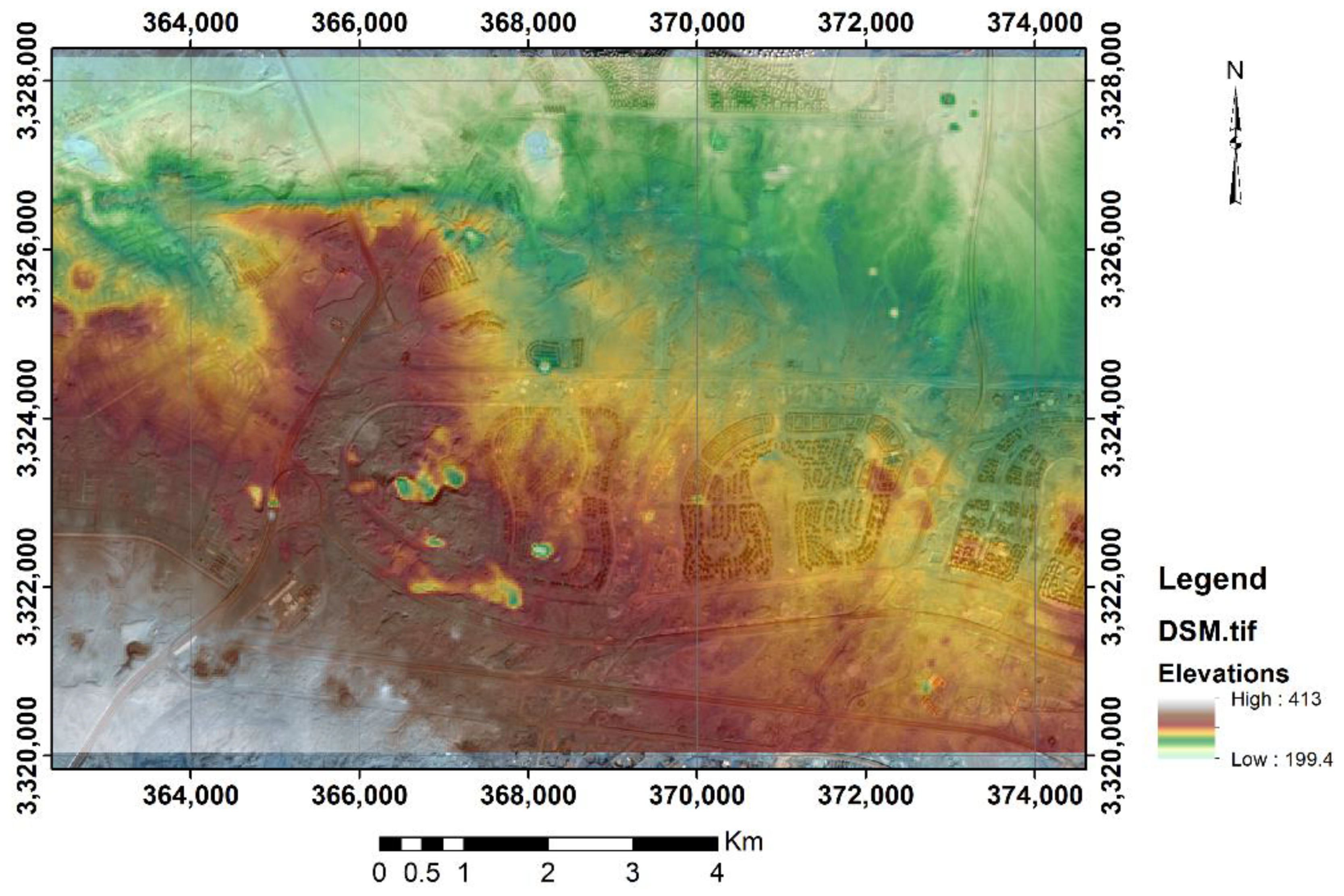
A DSM is a raster map representing the above-ground elements. A DEM, without objects such as trees and buildings, shows the shape of the bare earth. Many DSM and DEM data sources, varying from low- to high-resolution, have been produced in the past 30 years [23,24]. In particular, the Shuttle Radar Topography Mission (SRTM)-30 m and Advanced Spaceborne Thermal Emission and Reflection Radiometer (ASTER)-30 m are freely available and can be used for engineering applications, such as flood mapping. Data from the Advanced Land Observing Satellite (ALOS)-30 m DSM for the current study area can be downloaded from the ALOS website (https://scihub.copernicus.eu/ (accessed on 10 August 2021)). The region of interest (ROI) was clipped for the study area. Figure 3 shows the DSM with Sentinel-2 true color as the background.
2.4. Sentinel-1 Data
SAR penetrates clouds and dense vegetation, which makes it suitable for detecting water areas in all weather conditions. Sentinel-1 data, as a SAR product of the European Copernicus program, are freely accessible through the Copernicus Open Access Hub (https://step.esa.int/main/toolboxes/snap/ (accessed on 15 August 2021)), and cover the globe with a six-day temporal resolution and 10 m spatial resolution. The level-1 Interferometric Wide Swath (IW) product, acquired on 27 April 2018, was used to extract wet areas and estimate water depths during a flash flood in the study area. The Sentinel Application Platform (SNAP) software (https://step.esa.int/main/toolboxes/snap/ (accessed on 1 July 2021)) deals with all Sentinel-1 data products. Fundamental SAR image-processing steps include radiometric calibration, speckle filtering, terrain correction, and sigma naught () value calculation for vertical horizontal (VH) polarization. To improve the visualization of water areas, the pixel values were converted to backscattering in decibels (dB) of . The final SAR image was re-sampled to a 30 m ground sample distance (GSD) by nearest-neighbor interpolation and reprojected into the WGS84/UTM coordinate system.
2.5. Land Use
The land-use map was prepared using the ArcGIS 10.4 software by applying the maximum likelihood (ML) supervised classification method for the Sentinel-2 image, which entails four steps: (1) determine the number of layers; (2) select the training sample for each class; (3) estimate the mean vector and covariance matrix for each training sample layer; and (4) classify each pixel in the satellite image based on the covariance matrix and mean vector. Figure 4 shows the obtained classification land-use map. Table 1 shows that the overall classification accuracy was 87.1%, with a kappa coefficient of 0.815. The kappa coefficient indicates how well the classification results and truth values agree. A kappa value of 1 indicates complete agreement, whereas a value of 0 indicates no agreement.
2.6. Water Depth Extraction (Dependent Variable)
There were no direct measurements of water depth during flood times, so the DSM, land-use map, and rainfall data were used to analyze the unsteady flow using HEC-RAS 2D version 5.0.6. to estimate the water depth. The water depth from 24–27 April 2018 was generated using the modeling software. The digital map of the modeled maximum floodwater depth over 24–27 April is shown in Figure 5.
3. Methodology and Data Preparation
3.1. Research Methodology
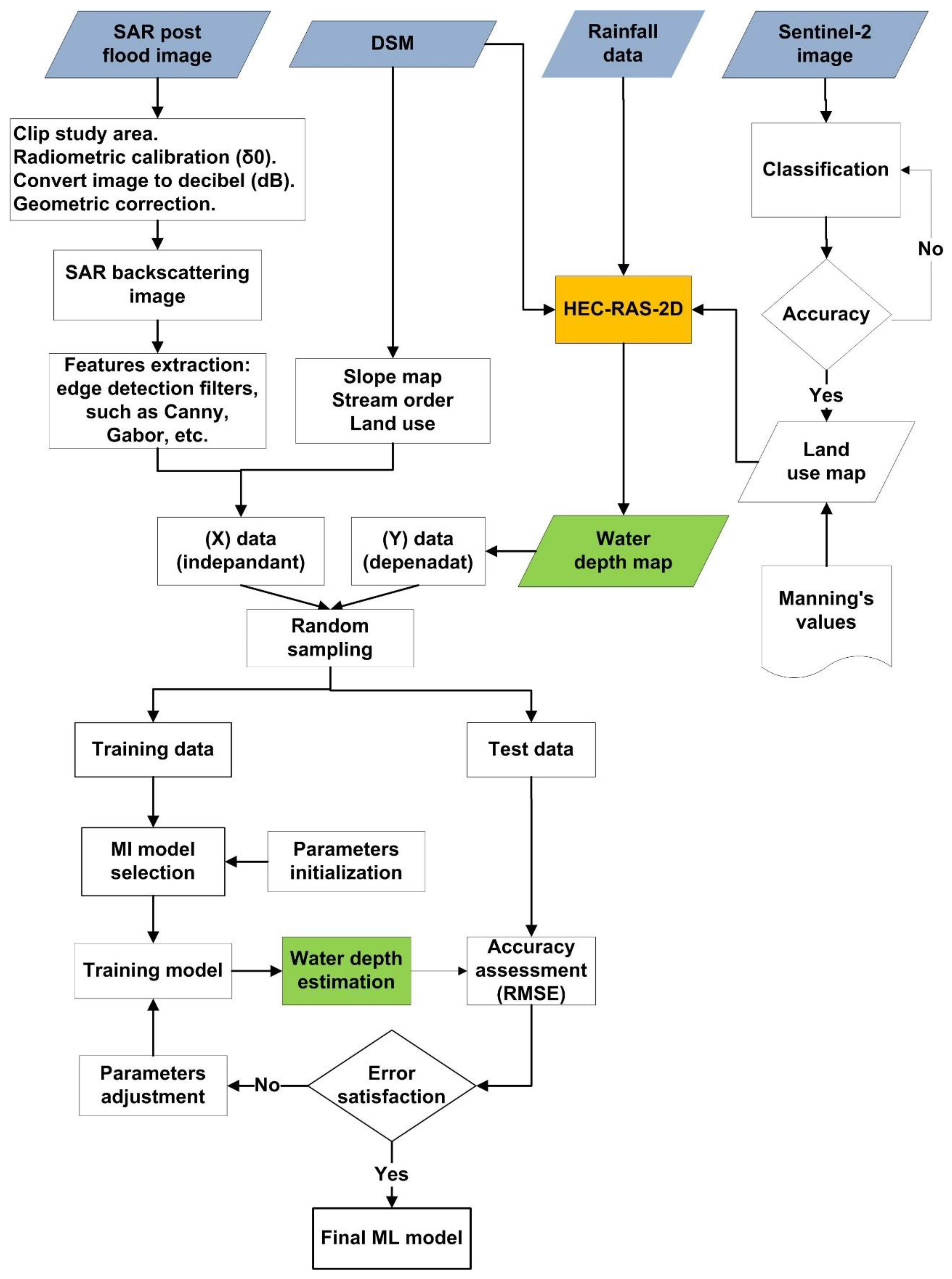
An ML algorithm consists of a dependent variable (Y) and an independent variable (X). In our study, Y represents floodwater depth, and X represents DSM, land-use map, and SAR image information. Water depth values will be predicted from a set of predictors or independent variables. In addition, the water depth and independent data images should match spatially and have the same resolution. The algorithm randomly divides the data into training and test sets before training the model. The ML algorithm updates its input parameters and generates the water depth model throughout the training phase. The model is validated by predicting new water depths using test data and calculating the root mean square error (RMSE) between the predicted and test values. Figure 6 shows a full flowchart for this procedure. I used 80% of the collected elevation data to train the algorithm, and 20% to validate the solutions.
3.2. Machine Learning Data Preparation
Any ML predictive modeling project is unique, but there are common basic processes, such as identifying the problem, preparing the data, and assessing and finalizing models [25]. The current project, predicting the depth of floodwater, involves a continuous output quantity rather than a discrete class label. Hence, I used ML regression modeling. Data preparation focuses on converting the gathered raw data to a format that can be used in modeling [26]. I selected appropriate metrics to evaluate the model and optimum hyperparameter tuning as part of the model evaluation. Independent variables (features) are used as the input for ML algorithms. The next two subsections describe how to obtain and manipulate the ML data input.
3.2.1. Dependent Feature Extraction and Preparation (Y)
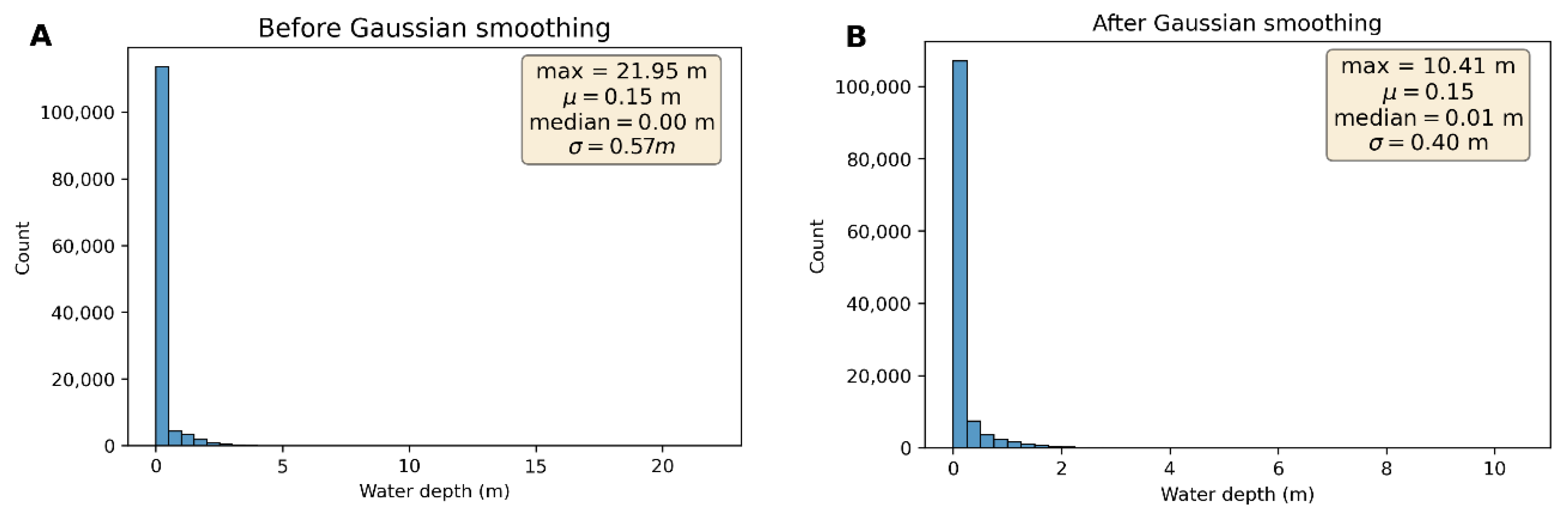
During the training and testing of the chosen ML algorithm, the water depth map displayed in Figure 5 (width = 458 and height = 274 pixels) was used as a dependent variable. Before data are used, they must be smoothed by a Gaussian filter to remove noise and outliers [27]. Figure 7 shows a histogram of water depth before and after Gaussian smoothing with σ = 1. Values were then reshaped from 2D (770 × 700) to a 1D Pandas DataFrame [28].
3.2.2. Independent Feature Extraction and Preparation (X)
The total number of independent features used to train the ML algorithms was 33, as extracted from SAR images, DSM models, and land-use maps. By applying some edge detection filters to the SAR image in addition to its original pixel values, 30 features were extracted. The earth surface slope and stream order calculated based on a DSM map were added as two more features. The land-use map (Figure 4) was used as another independent feature. Raster images were resized to a raster size of 458 × 274 pixels and a resolution of 30 m before any computations. The total number of sample datasets used after reshaping the 2D raster maps to a 1D vector data form was 125,492.
3.2.3. Independent Feature Extraction Algorithms and Methods
The digital filters and equations used to collect independent variables for input to ML algorithms will be discussed.
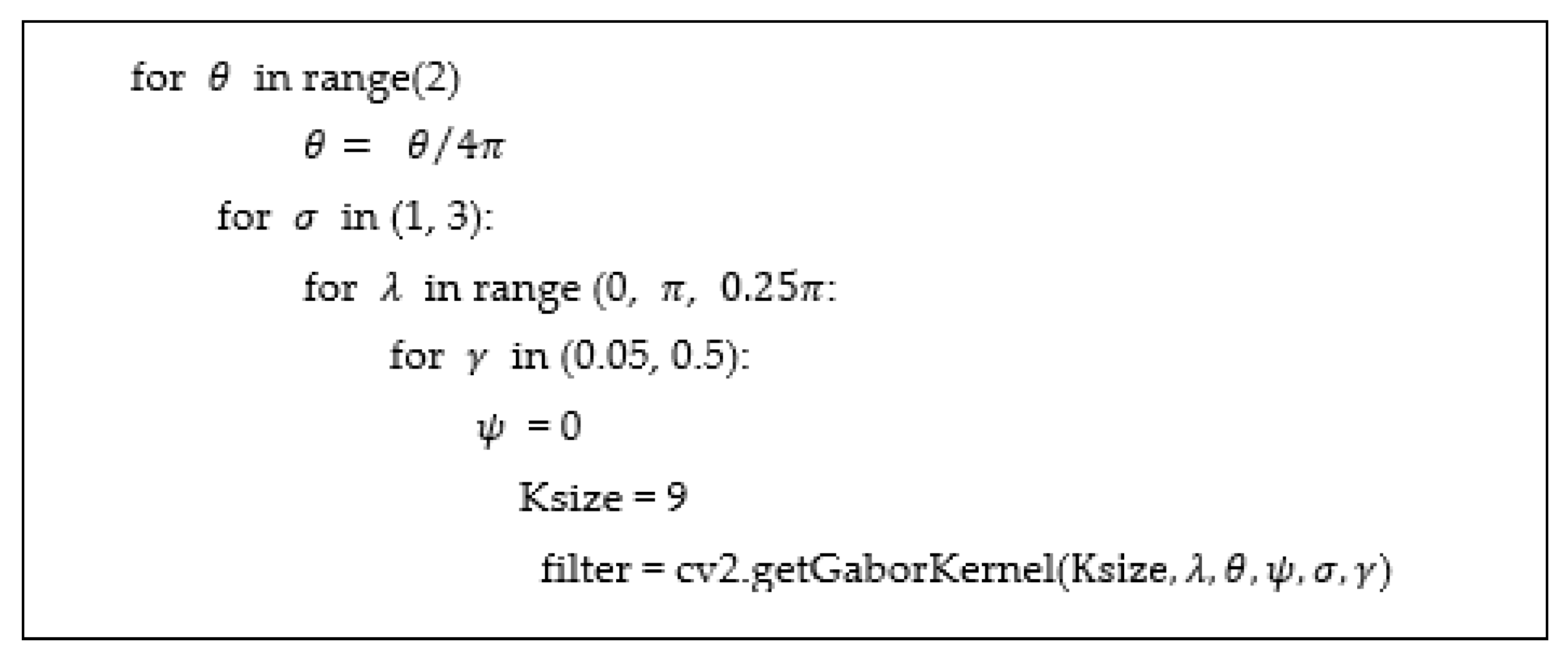
Raster SAR images represent pixels with a 30 m ground sample distance, and each pixel has a value for polarization. Gabor kernel values and those from additional edge detection filters, such as Canny, Sobel, Roberts, and Prewitt, were estimated as independent features based on SAR image pixel values. Gabor filters are directional filters used for edge detection and analysis if an image has a sudden sharp increase [29,30], and are determined as
where
λ is the wavelength, σ is the standard deviation of the Gaussian function in the x and y directions, θ indicates the orientation of the filter, and ψ is the phase offset. The shape of a Gabor filter depends on the aspect ratio γ. If γ is equal to one, then the filter appears as a circle. The shape of the filter will gradually change from an ellipsoid to a straight line when γ is close to zero [31]. By varying the Gabor parameters λ, θ, ψ, σ, and γ, different orientations are used to analyze the texture or obtain features from images. Figure 8 shows the source python code used to extract the Gabor filter parameters using multi for loops. Accordingly, 32 Gabor labels were generated using a Python code, each having the values of its own parameters.
The OpenCV open-source code library was used to calculate the values of the Gabor features and other edge detection filters [32,33].
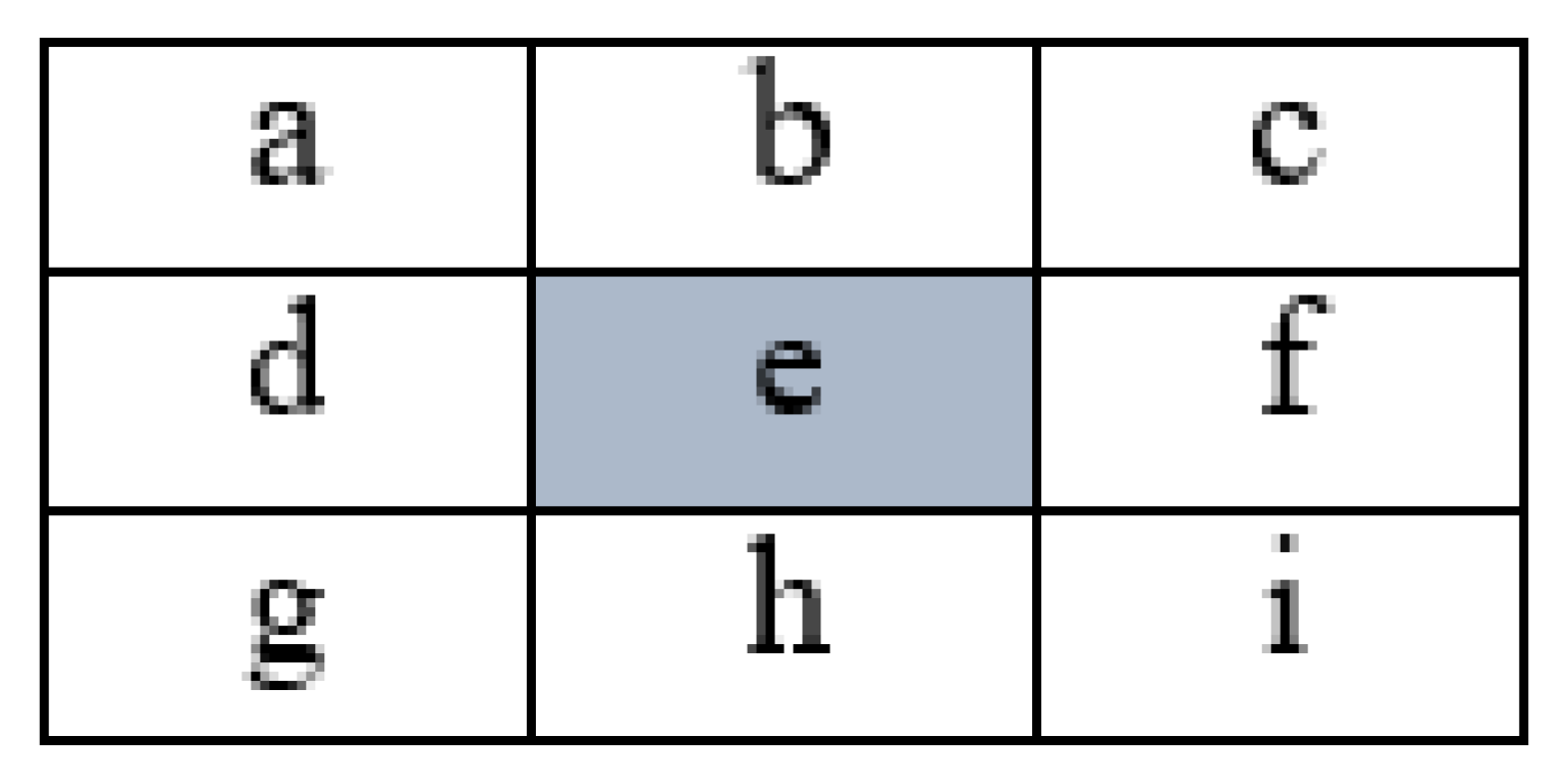
The surface slope indicates the steepness of the ground’s surface. The slope between two points on the Earth’s surface can be calculated by dividing their elevation difference by the horizontal distance between them. For the DSM surface, the surface slope in degrees can be calculated as
where is the perpendicular rate of change for the center cell of a moving 3 × 3 pixel window for grid-based DSM [34,35,36]. Figure 9 shows the pixel values of a moving 3 × 3 window, where the neighbors of the center cell e are identified by the letters a to i. The perpendicular rate of change for the x and y directions is calculated as
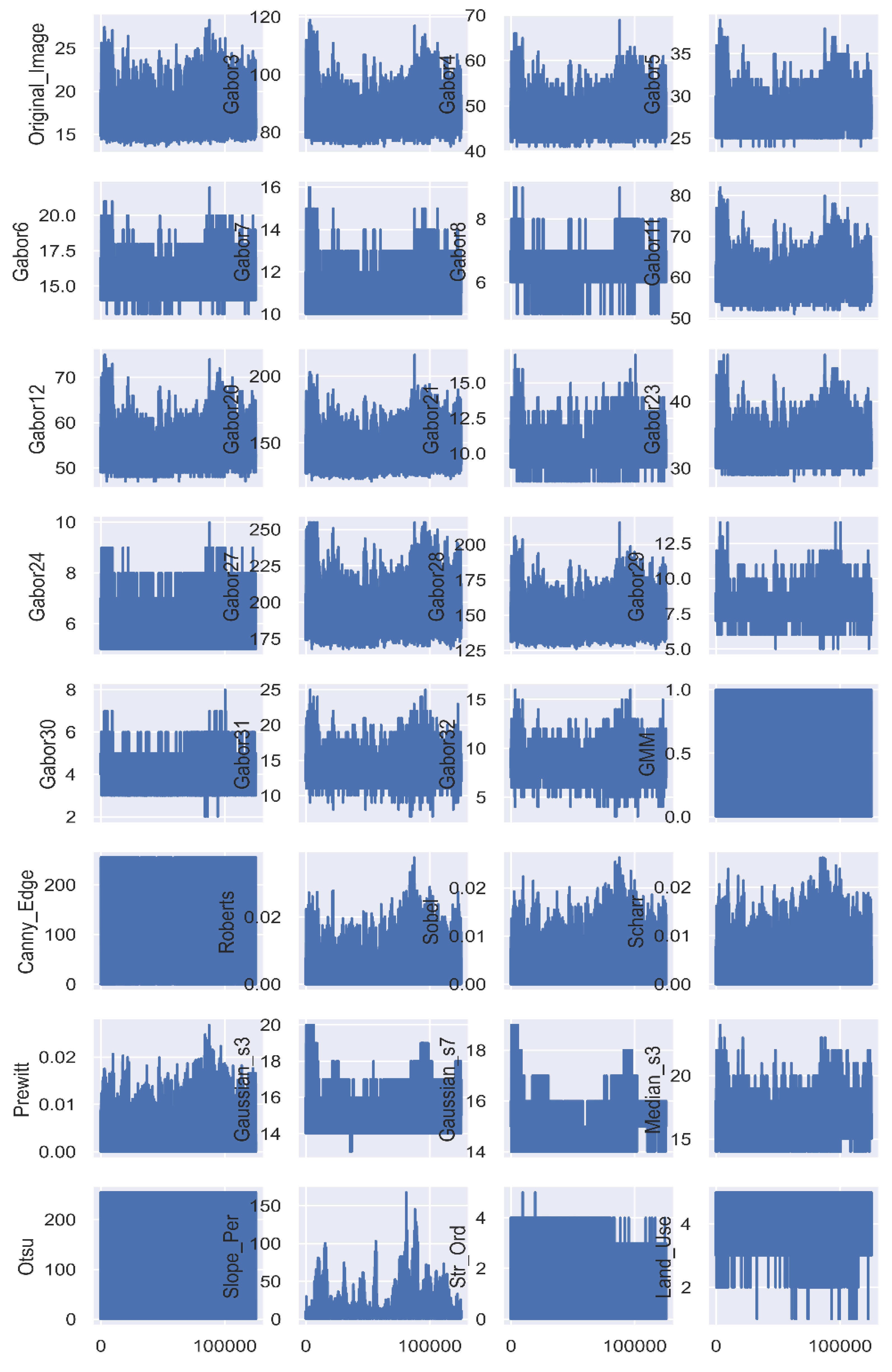
The ArcGIS 10.7 software was used to calculate the slope for the current study. In hydrology, the stream or waterbody order is a positive, whole number that indicates the degree of splitting in a stream channel. Using ArcGIS software version 10.7, a raster image representing the stream order for the current study site was delineated from the DSM [37]. Subsequently, Sentinel-2 remote sensing satellite photos were classified to obtain land-cover features, including water, roads, green areas, buildings, and bare soil, identified by integers 1–5, respectively. Figure 10 and Table 2 show the 32 features extracted to train the ML algorithms and predict water depths. Some features were removed because their output values were constant at a given value and did not vary at each pixel. As a result, the overall number of features dropped from 33 to 32.
The collected data were randomly divided into a training dataset (80%, n = 100,393) to generate water depths using various interpolation ML algorithms, and a validation dataset (20%, n = 25,099) to calculate the accuracy of each model.
3.3. Quality Assessment
Of the measures for assessing derived ML models, RMSE is commonly used when comparing predicted and actual independent values. The RMSE uses the squared error; hence, greater errors have a stronger influence. The RMSE is calculated as
where and are the actual and predicted water depths, respectively. The RMSE was used to compare ML models.
4. Results
Several ML regression techniques, including support vector machine (SVR), random forest (RF), k-nearest neighbors (KNR), and extreme gradient boosting (Xgboost), have been suggested for the spatial interpolation of environmental variables, and several hybrid methods have been adopted.
4.1. Machine Learning Hyperparameter Tuning
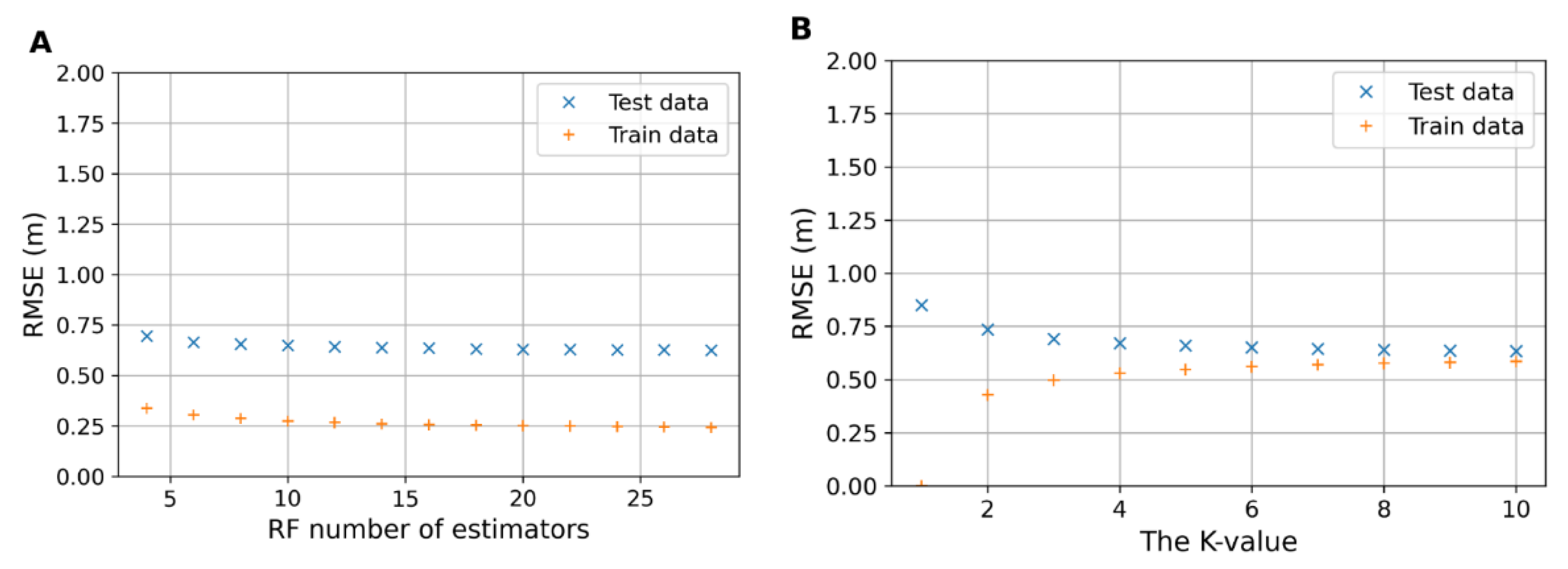
The precision and accuracy of ML algorithms are determined by the input variables. Hyperparameter tuning is the process of finding the optimal hyperparameters to achieve high precision and accuracy. GridSearch is a function in the Scikit-learn package that is used to find the optimum parameters by building and evaluating multiple models with different hyperparameter combinations. Other parameter tuning methods, such as Random search and Bayesian optimization, can be implemented using Scikit-learn [38]. Figure 11A illustrates the influence of the number of estimators on the RF model’s accuracy, which was steady and did not improve after using more than 15 estimators. Figure 11B depicts the impact of using the number of nearby points on the tree model’s accuracy. The accuracy of the KNR model was stable and did not improve after employing more than eight neighboring points.
The optimal results can be summarized as follows: the best number of estimators for the RF algorithm was 12; the k-value for KNN was 7; for xgboost, the optimal number of estimators was 60; and for SVR, the kernel was ‘C’: 1, ‘epsilon’: 0.02, ‘gamma’: 0.01, ‘kernel’: ‘rbf’. The C value was used to adjust the error or margin, gamma was used with Gaussian rbf kernel, and epsilon was used to smooth the algorithm response.
4.2. Accuracy of Obtained ML Algorithms
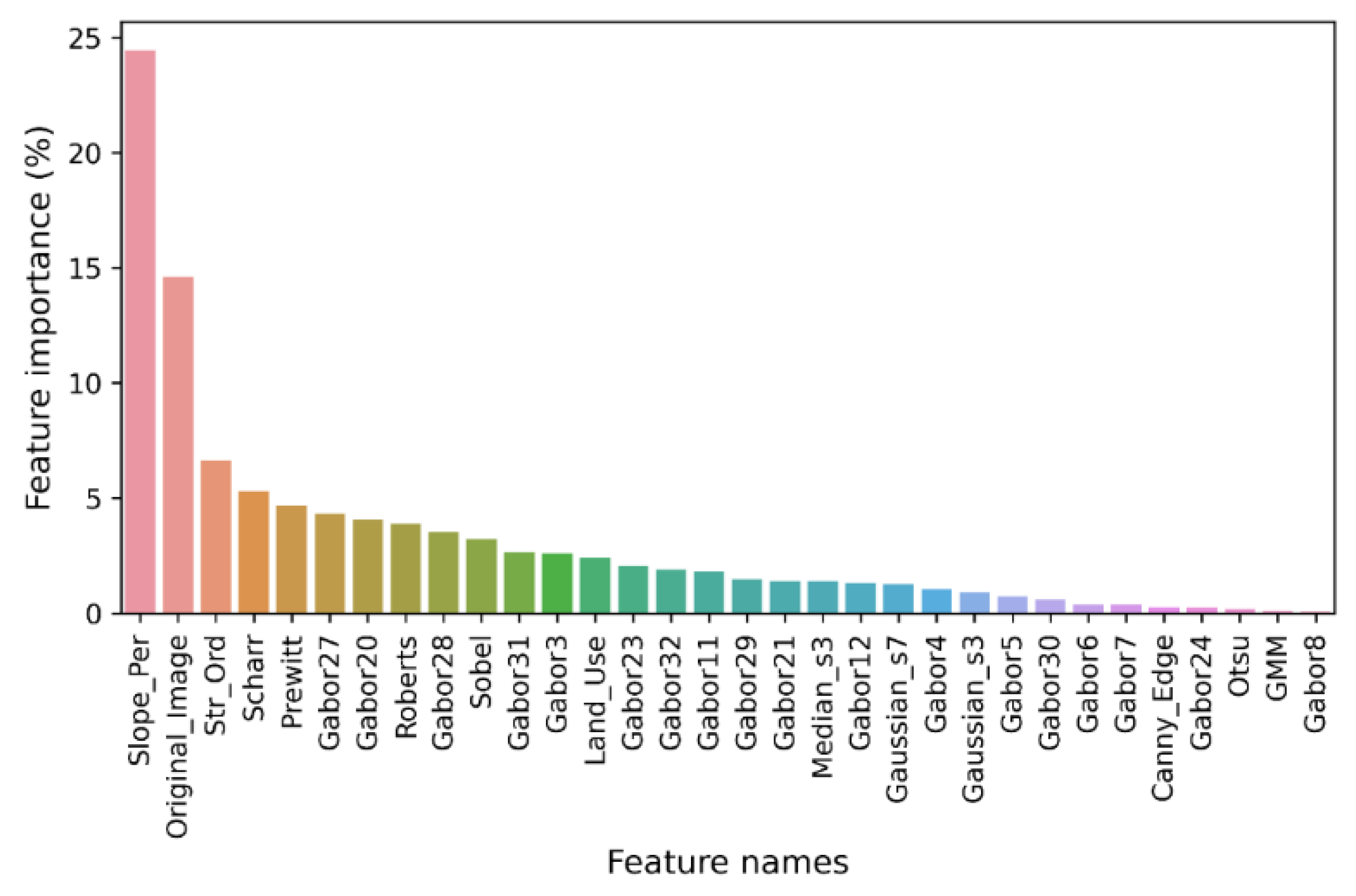
When the number of input features is large, it is preferable to use the most significant ones during ML training to reduce processing time, enhance output accuracy, and make model interpretation and understanding easier. Some ML algorithms, such as RFR, assess the effectiveness of their input features [39,40]. Figure 12 shows the degree of importance of each data feature.
5. Discussion
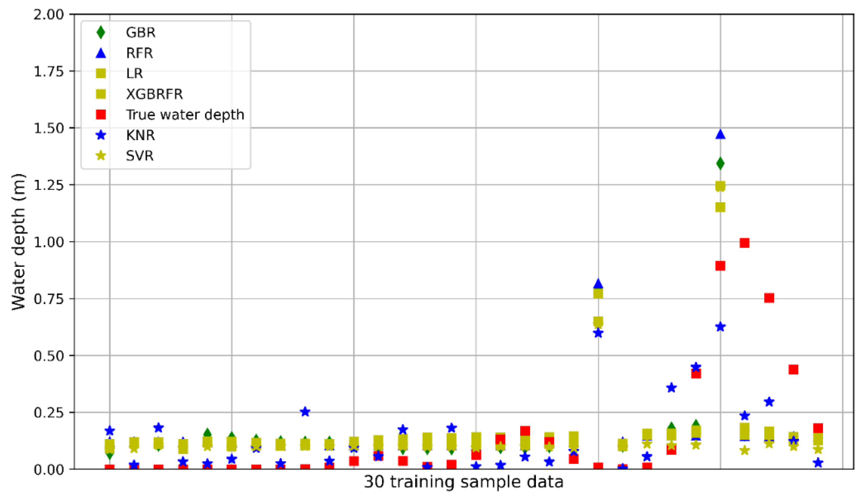
As shown by the comparison results, the most effective feature was the surface slope, followed by the SAR backscattering values. Figure 13 shows 30 sample data outputs for the different used algorithms.
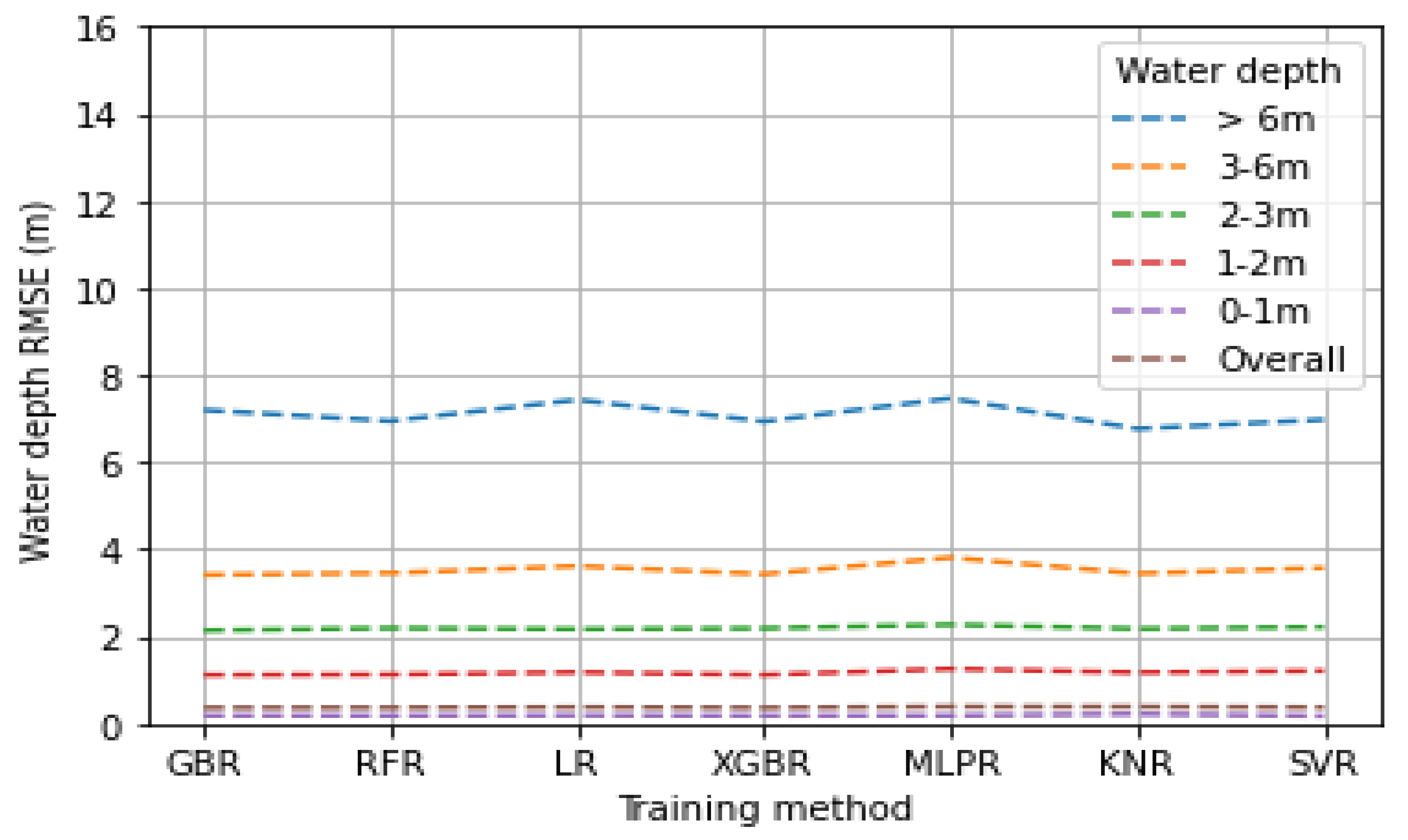
Although the RMSE is heavily influenced by the distribution of validation points, it is nevertheless a useful metric for assessing the accuracy of predicted water depths. The RMSEs of multiple water depth ranges are shown in Table 3. The GBR and XGBRFR approaches had the best accuracy for the overall test data, and MLPR and KNR had the worst accuracy. The SVR and XGBR algorithms had the most accurate models, with RMSE of 0.20 m at water depths of 0–1 m, contributing to 96% of the test data. Figure 14 shows the RMSE values for all conducted regression algorithms at different water depths.
Figure 14 shows the RMSE values for all conducted regression algorithms at different water depths. Previous methods depended on DEM and SAR data and could only be used for flat or gently sloping terrain [41]. The technique I propose is straightforward because it works on any terrain and simply requires SAR and DEM data.
6. Conclusions
In this study, water depth estimation after a flash flood event in New Cairo City, Egypt, was investigated using multiple ML algorithms. Several training datasets and ML techniques were combined. The backscattering spectral band of the SAR data was used to extract features to be used as independent inputs for ML algorithms. The water depth (dependent input) was extracted by hydrodynamic HEC-RAS 2D software to obtain 250,099 data samples and 33 features to train and validate the used algorithms; 80% of the input data were used for training and 20% for testing. I compared the accuracy of the obtained models. The water depths were classified into five groups, and 96.27% of total water depths fell between 0 and 1 m. All ML methods produced RMSE values of 0.18–0.22 m over this water depth range. The XGBR and SVR models had the best accuracy, and the KNR model had the worst. For deep water depths (more than 6 m), four sample datasets were found. Therefore, the accuracy of all approaches was reduced, as the RMSE values ranged from 7.20 to 6.77 m. Moreover, for all water depths, the prediction results were more consistent, and the GBR and XGBR models achieved the best accuracy. For effective forecasting of water depth from satellite data to build an emergency plan in case of floods, I recommend integrating various training datasets and machine learning algorithms.
Funding
The project was funded by the Deanship of Scientific Research at Najran University, project number (NU/SERC/10/550).
Institutional Review Board Statement
Not applicable.
Informed Consent Statement
Not applicable.
Data Availability Statement
The data that support the findings of this study are available from the author upon reasonable request.
Acknowledgments
The authors are thankful to the Deanship of Scientific Research at Najran University for funding this work under the General Research Funding program grant code (NU/SERC/10/550).
Conflicts of Interest
The authors declare no conflict of interest.
References
- Townsend, P.A.; Walsh, S.J. Modeling floodplain inundation using an integrated GIS with radar and optical remote sensing. Geomorphology 1998, 21, 295–312. [Google Scholar] [CrossRef]
- Vishnu, C.L.; Sajinkumar, K.S.; Oommen, T.; Coffman, R.A.; Thrivikramji, K.P.; Rani, V.R.; Keerthy, S. Satellite-based assessment of the August 2018 flood in parts of Kerala, India. Geomat. Nat. Hazards Risk 2019, 10, 758–767. [Google Scholar] [CrossRef] [Green Version]
- Irwin, K.; Beaulne, D.; Braun, A.; Fotopoulos, G. Fusion of SAR, optical imagery and airborne LiDAR for surface water detection. Remote Sens. 2017, 9, 890. [Google Scholar] [CrossRef] [Green Version]
- Musa, Z.N.; Popescu, I.; Mynett, A. A review of applications of satellite SAR, optical, altimetry and DEM data for surface water modelling, mapping and parameter estimation. Hydrol. Earth Syst. Sci. 2015, 19, 3755–3769. [Google Scholar] [CrossRef] [Green Version]
- Bovenga, F.; Bovenga, F.; Belmonte, A.; Refice, A.; Pasquariello, G.; Nutricato, R.; Nitti, D.O.; Chiaradia, M.T. Performance analysis of satellite missions for multi-temporal SAR interferometry. Sensors 2018, 18, 1359. [Google Scholar] [CrossRef] [PubMed] [Green Version]
- Bioresita, F.; Puissant, A.; Stumpf, A.; Malet, J.P. A method for automatic and rapid mapping of water surfaces from Sentinel-1 imagery. Remote Sens. 2018, 10, 217. [Google Scholar] [CrossRef] [Green Version]
- Alsdorf, D.E.; Rodríguez, E.; Lettenmaier, D.P. Measuring surface water from space. Rev. Geophys. 2007, 45. [Google Scholar] [CrossRef]
- Yalcin, E. Two-dimensional hydrodynamic modelling for urban flood risk assessment using unmanned aerial vehicle imagery: A case study of Kirsehir, Turkey. J. Flood Risk Manag. 2019, 12, e12499. [Google Scholar] [CrossRef]
- Costabile, P.; Costanzo, C.; Ferraro, D.; Barca, P. Is HEC-RAS 2D accurate enough for storm-event hazard assessment? Lessons learnt from a benchmarking study based on rain-on-grid modelling. J. Hydrol. 2021, 603, 126962. [Google Scholar] [CrossRef]
- El Afandi, G.; Morsy, M. Developing an Early Warning System for Flash Flood in Egypt: Case Study Sinai Peninsula. In Advances in Science, Technology and Innovation; Springer: Berlin/Heidelberg, Germany, 2020; pp. 45–60. [Google Scholar]
- Abdeldayem, O.M.; Eldaghar, O.; KMostafa, M.; MHabashy, M.; Hassan, A.A.; Mahmoud, H.; Morsy, K.M.; Abdelrady, A.; Peters, R.W. Mitigation plan and water harvesting of flashflood in arid rural communities using modelling approach: A case study in Afouna village, Egypt. Water 2020, 12, 2565. [Google Scholar] [CrossRef]
- Sadek, M.; Li, X.; Mostafa, E.; Dossou, J.F. Monitoring flash flood hazard using modeling-based techniques and multi-source remotely sensed data: The case study of Ras Ghareb City, Egypt. Arab. J. Geosci. 2021, 14, 2030. [Google Scholar] [CrossRef]
- Elkhrachy, I.; Pham, Q.B.; Costache, R.; Mohajane, M.; Rahman, K.U.; Shahabi, H.; Linh, N.T.T.; Anh, N.T. Sentinel-1 remote sensing data and Hydrologic Engineering Centres River Analysis System two-dimensional integration for flash flood detection and modelling in New Cairo City, Egypt. J. Flood Risk Manag. 2021, 14, e12692. [Google Scholar] [CrossRef]
- El-Haddad, B.A.; Youssef, A.M.; Pourghasemi, H.R.; Pradhan, B.; El-Shater, A.H.; El-Khashab, M.H. Flood susceptibility prediction using four machine learning techniques and comparison of their performance at Wadi Qena Basin, Egypt. Nat. Hazards 2021, 105, 83–114. [Google Scholar] [CrossRef]
- El-Magd, S.A.A.; Pradhan, B.; Alamri, A. Machine learning algorithm for flash flood prediction mapping in Wadi El-Laqeita and surroundings, Central Eastern Desert, Egypt. Arab. J. Geosci. 2021, 14, 323. [Google Scholar] [CrossRef]
- Mudashiru, R.B.; Sabtu, N.; Abustan, I. Quantitative and semi-quantitative methods in flood hazard/susceptibility mapping: A review. Arab. J. Geosci. 2021, 14, 941. [Google Scholar] [CrossRef]
- Friedman, J.; Hastie, T.; Tibshirani, R. The Elements of Statistical Learning; Springer series in statistics; Springer: New York, NY, USA, 2001; Volume 1, No. 10. [Google Scholar]
- Ghorpade, P.; Gadge, A.; Lende, A.; Chordiya, H.; Gosavi, G.; Mishra, A.; Hooli, B.; Ingle, Y.S.; Shaikh, N. Flood Forecasting Using Machine Learning: A Review. In Proceedings of the 2021 8th International Conference on Smart Computing and Communications: Artificial Intelligence, AI Driven Applications for a Smart World, ICSCC, Kochi, Kerala, India, 1–3 July 2021; Volume 2021, pp. 32–36. [Google Scholar] [CrossRef]
- Breiman, L. Random forests. Mach. Learn. 2001, 45, 5–32. [Google Scholar] [CrossRef] [Green Version]
- Sekulić, A.; Kilibarda, M.; Heuvelink, G.; Nikolić, M.; Bajat, B. Random forest spatial interpolation. Remote Sens. 2020, 12, 1687. [Google Scholar] [CrossRef]
- Breiman, L. Bagging predictors. Mach. Learn. 1996, 24, 123–140. [Google Scholar] [CrossRef] [Green Version]
- Wu, Z.; Mao, Z.; Shen, W. Integrating Multiple Datasets and Machine Learning Algorithms for Satellite-Based Bathymetry in Seaports. Remote Sens. 2021, 13, 4328. [Google Scholar] [CrossRef]
- Elkhrachy, I. Vertical accuracy assessment for SRTM and ASTER Digital Elevation Models: A case study of Najran city, Saudi Arabia. Ain Shams Eng. J. 2018, 9, 1807–1817. [Google Scholar] [CrossRef]
- Mesa-Mingorance, J.L.; Ariza-López, F.J. Accuracy assessment of digital elevation models (DEMs): A critical review of practices of the past three decades. Remote Sens. 2020, 12, 2630. [Google Scholar] [CrossRef]
- Kuhn, M.; Johnson, K. Applied Predictive Modeling; Springer: Berlin/Heidelberg, Germany, 2013; Volume 26. [Google Scholar]
- Liu, H. Feature Engineering for Machine Learning and Data Analytics; O’Reilly Media, Inc.: Sevastopol, CA, USA, 2018. [Google Scholar]
- Davies, E.R. Machine Vision: Theory, Algorithms, Practicalities; Elsevier: Amsterdam, The Netherlands, 2004. [Google Scholar]
- McKinney, W.; Team, P.D. Pandas-Powerful python data analysis toolkit. Pandas—Powerful Python Data Anal. Toolkit 2015, 1625. Available online: https://pandas.pydata.org/docs/pandas.pdf (accessed on 15 September 2021).
- Fogel, I.; Sagi, D. Gabor filters as texture discriminator. Biol. Cybern. 1989, 61, 103–113. [Google Scholar] [CrossRef]
- Grigorescu, S.E.; Petkov, N.; Kruizinga, P. Comparison of texture features based on Gabor filters. IEEE Trans. Image Process. 2002, 11, 1160–1167. [Google Scholar] [CrossRef] [PubMed] [Green Version]
- Palm, C.; Lehman, T. Classification of color textures by gabor filtering. Mach. Graph. Vis. 2002, 11, 195–220. [Google Scholar]
- OpenCV, L. Computer Vision with the OpenCV Library; O’Reilly Media, Inc.: Sevastopol, CA, USA, 2008. [Google Scholar]
- Pedregosa, F.; Varoquaux, G.; Gramfort, A.; Michel, V.; Thirion, B.; Grisel, O.; Blondel, M.; Prettenhofer, P.; Weiss, R.; Dubourg, V.; et al. Scikit-learn: Machine learning in Python. J. Mach. Learn. Res. 2011, 12, 2825–2830. Available online: http://jmlr.csail.mit.edu/papers/v12/pedregosa11a.html%5Cnhttp://arxiv.org/abs/1201.0490 (accessed on 15 September 2021).
- Skidmore, A.K. A comparison of techniques for calculating gradient and aspect from a gridded digital elevation model. Int. J. Geogr. Inf. Syst. 1989, 3, 323–334. [Google Scholar] [CrossRef]
- Zhou, Q.; Liu, X. Analysis of errors of derived slope and aspect related to DEM data properties. Comput. Geosci. 2004, 30, 369–378. [Google Scholar] [CrossRef]
- Cone, J. Principles of Geographical Information Systems by Peter A; Oxford University Press: Oxford, UK, 1998; Volume 54. [Google Scholar]
- Jenson, S.K. Applications of hydrologic information automatically extracted from digital elevation models. Hydrol. Process. 1991, 5, 31–44. [Google Scholar] [CrossRef]
- Buitinck, L.; Louppe, G.; Blondel, M.; Pedregosa, F.; Mueller, A.; Grisel, O.; Niculae, V.; Prettenhofer, P.; Gramfort, A.; Grobler, J.; et al. API design for machine learning software: Experiences from the scikit-learn project. arXiv 2013, arXiv:1309.0238. [Google Scholar]
- Hall, M.A. Correlation-based Feature Selection for Discrete and Numeric Class Machine Learning. Eff. Br. Mindfulness Interv. Acute Pain ExAn. Exam. Individ. Differ. 2015, 1, 1689–1699. Available online: https://researchcommons.waikato.ac.nz/handle/10289/1024 (accessed on 21 August 2021).
- Genuer, R.; Poggi, J.M.; Tuleau-Malot, C. Variable selection using random forests. Pattern Recognit. Lett. 2010, 31, 2225–2236. [Google Scholar] [CrossRef] [Green Version]
- Cian, F.; Marconcini, M.; Ceccato, P.; Giupponi, C. Flood depth estimation by means of high-resolution SAR images and lidar data. Nat. Hazards Earth Syst. Sci. 2018, 18, 3063–3084. [Google Scholar] [CrossRef] [Green Version]
Figure 1.
Ten-meter spatial resolution true-color image based on Sentinel-2 satellite data for the study area.
Figure 1.
Ten-meter spatial resolution true-color image based on Sentinel-2 satellite data for the study area.

Figure 2.
Rainfall intensity during a flash flood on 24 April 2018.

Figure 3.
DSM of study area projected by WGS84/UTM coordinate system.

Figure 4.
Land-use map of the study area.

Figure 5.
Simulated water depth using HEC-RAD 2D.

Figure 6.
Flowchart of water depth estimation.

Figure 7.
Histograms of the dependent variable (water depth): (A) before smoothing; (B) after smoothing.
Figure 7.
Histograms of the dependent variable (water depth): (A) before smoothing; (B) after smoothing.

Figure 8.
Parameters of Gabor filters.

Figure 9.
Moving 3 × 3-pixel window to calculate the surface slope.

Figure 10.
Features used to model water depth.

Figure 11.
ML hyperparameter tuning: (A) number of estimators in RF; (B) k-values for KNR.

Figure 12.
Input feature importance.

Figure 13.
Input feature importance.

Figure 14.
Accuracy of different regression algorithms.


Table 1.
Classification accuracy of land-use map.
| Bare Soil | Buildings | Green | Roads | Water | Sum | User’s Accuracy | |
|---|---|---|---|---|---|---|---|
| Bare soil | 107 | 0 | 1 | 3 | 2 | 113 | 94.7% |
| Buildings | 2 | 42 | 1 | 2 | 1 | 48 | 87.5% |
| Green | 1 | 1 | 6 | 1 | 1 | 10 | 60.0% |
| Roads | 2 | 1 | 3 | 28 | 2 | 36 | 77.8% |
| Water | 1 | 0 | 1 | 2 | 6 | 10 | 60.0% |
| Sum | 113 | 44 | 12 | 36 | 12 | 217 | |
| Producer’s accuracy | 94.7% | 95.5% | 50.0% | 77.8% | 50.0% | ||
| Total Accuracy | 87.1% | ||||||
| a | 26,714 | ||||||
| b | 32,790 | ||||||
| Kappa | 81.5% |
Table 2.
Sample of the extracted feature values.
| ML Data | Based On: | Features | Pixel ID (Sample Number) | ||||
|---|---|---|---|---|---|---|---|
| ID | Filter | 1 | 2 | 125491 | 125492 | ||
| Independent data (X) | SAR image | 1 | Original Image | 19.23 | 18.45 | 16.59 | 15.29 |
| 2 | Gabor3 | 91.00 | 90.00 | 84.00 | 81.00 | ||
| 3 | Gabor4 | 51.00 | 51.00 | 46.00 | 44.00 | ||
| 4 | Gabor5 | 29.00 | 29.00 | 27.00 | 26.00 | ||
| 5 | Gabor6 | 17.00 | 16.00 | 15.00 | 14.00 | ||
| 6 | Gabor7 | 12.00 | 12.00 | 11.00 | 11.00 | ||
| 7 | Gabor8 | 7.00 | 7.00 | 6.00 | 6.00 | ||
| 8 | Gabor11 | 62.00 | 62.00 | 58.00 | 55.00 | ||
| 9 | Gabor12 | 57.00 | 57.00 | 53.00 | 51.00 | ||
| 10 | Gabor19 | 255.00 | 255.00 | 255.00 | 255.00 | ||
| 11 | Gabor20 | 156.00 | 155.00 | 140.00 | 132.00 | ||
| 12 | Gabor21 | 10.00 | 10.00 | 10.00 | 10.00 | ||
| 13 | Gabor23 | 34.00 | 34.00 | 32.00 | 31.00 | ||
| 14 | Gabor24 | 7.00 | 7.00 | 6.00 | 6.00 | ||
| 15 | Gabor27 | 206.00 | 205.00 | 188.00 | 180.00 | ||
| 16 | Gabor28 | 159.00 | 158.00 | 144.00 | 136.00 | ||
| 17 | Gabor29 | 8.00 | 7.00 | 8.00 | 8.00 | ||
| 18 | Gabor30 | 4.00 | 4.00 | 4.00 | 4.00 | ||
| 19 | Gabor31 | 14.00 | 14.00 | 14.00 | 13.00 | ||
| 20 | Gabor32 | 8.00 | 8.00 | 8.00 | 8.00 | ||
| 21 | GMM | 1.00 | 0.00 | 0.00 | 0.00 | ||
| 22 | Canny Edge | 0.00 | 0.00 | 0.00 | 0.00 | ||
| 23 | Roberts | 0.01 | 0.00 | 0.00 | 0.00 | ||
| 24 | Sobel | 0.01 | 0.00 | 0.00 | 0.00 | ||
| 25 | Scharr | 0.01 | 0.00 | 0.00 | 0.00 | ||
| 26 | Prewitt | 0.01 | 0.00 | 0.00 | 0.00 | ||
| 27 | Gaussian s3 | 15.00 | 15.00 | 15.00 | 14.00 | ||
| 28 | Gaussian s7 | 15.00 | 15.00 | 15.00 | 15.00 | ||
| 29 | Median s3 | 18.00 | 18.00 | 16.00 | 15.00 | ||
| 30 | Otsu | 255.00 | 255.00 | 0.00 | 0.00 | ||
| 31 | Slope_Per | 6.25 | 6.09 | 4.48 | 2.98 | ||
| 32 | Str_Ord | 0.00 | 0.00 | 0.00 | 0.00 | ||
| 33 | Land_Use | 3.00 | 3.00 | 3.00 | 3.00 | ||
| 1 | Water_depth | 0.17 | 0.16 | 0.10 | 0.12 | ||
| 31 | Slope_Per | 6.25 | 6.09 | 4.48 | 2.98 | ||
| DSM image | 32 | Str_Ord | 0.00 | 0.00 | 0.00 | 0.00 | |
| Sentinel-2 image | 33 | Land_Use | 3.00 | 3.00 | 3.00 | 3.00 | |
| Dependent data (Y) | HEC-RAS results | 1 | Water_depth | 0.17 | 0.16 | 0.10 | 0.12 |
Table 3.
Comparison of RMSE and regression techniques at various water depths.
| Water Depth | Number of Points | Percentages (%) | RMSE (m) ML Algorithm | ||||||
|---|---|---|---|---|---|---|---|---|---|
| GBR | RFR | LR | XGBR | MLPR | KNR | SVR | |||
| >6 m | 4 | 0.02 | 7.20 | 6.95 | 7.43 | 6.94 | 7.47 | 6.77 | 6.98 |
| 3–6 m | 56 | 0.22 | 3.42 | 3.46 | 3.62 | 3.43 | 3.81 | 3.44 | 3.57 |
| 2–3 m | 157 | 0.63 | 2.14 | 2.19 | 2.17 | 2.19 | 2.27 | 2.18 | 2.22 |
| 1–2 m | 718 | 2.86 | 1.12 | 1.13 | 1.18 | 1.12 | 1.26 | 1.17 | 1.21 |
| 0–1 m | 24,164 | 96.27 | 0.19 | 0.19 | 0.19 | 0.18 | 0.19 | 0.22 | 0.18 |
| Overall | 25,099 | 100 | 0.36 | 0.37 | 0.38 | 0.36 | 0.39 | 0.39 | 0.37 |
Publisher’s Note: MDPI stays neutral with regard to jurisdictional claims in published maps and institutional affiliations. |
© 2022 by the author. Licensee MDPI, Basel, Switzerland. This article is an open access article distributed under the terms and conditions of the Creative Commons Attribution (CC BY) license (https://creativecommons.org/licenses/by/4.0/).
Share and Cite
MDPI and ACS Style
Elkhrachy, I. Flash Flood Water Depth Estimation Using SAR Images, Digital Elevation Models, and Machine Learning Algorithms. Remote Sens. 2022, 14, 440. https://doi.org/10.3390/rs14030440
AMA Style
Elkhrachy I. Flash Flood Water Depth Estimation Using SAR Images, Digital Elevation Models, and Machine Learning Algorithms. Remote Sensing. 2022; 14(3):440. https://doi.org/10.3390/rs14030440
Chicago/Turabian StyleElkhrachy, Ismail. 2022. "Flash Flood Water Depth Estimation Using SAR Images, Digital Elevation Models, and Machine Learning Algorithms" Remote Sensing 14, no. 3: 440. https://doi.org/10.3390/rs14030440
Note that from the first issue of 2016, this journal uses article numbers instead of page numbers. See further details here.