Ice Cover, Subglacial Landscape, and Estimation of Bottom Melting of Mac. Robertson, Princess Elizabeth, Wilhelm II, and Western Queen Mary Lands, East Antarctica

Abstract

This study demonstrates the results of Russian airborne radio-echo sounding (RES) investigations and also seismic reflection soundings carried out in 1971–2020 over a vast area of coastal part of East Antarctica. It is the first comprehensive summary mapping of these data. Field research, equipment, errors of initial RES data, and methods of gridding are discussed. Ice thickness, ice base elevation, and bedrock topography are presented. The ice thickness across the research area varies from a few meters to 3620 m, and is greatest in the local subglacial depressions. The average thickness is about 1220 m. The total volume of the ice is about 710,500 km${}^3$. The bedrock heights vary from 2860 m below sea level in the ocean bathyal zone to 2040 m above sea level in the Grove Mountains area (4900 m relief). The main directions of the bedrock orographic forms are concentrated mostly in three intervals: 345${}^{\circ }$–30${}^{\circ }$, 45${}^{\circ }$–70${}^{\circ }$, and 70${}^{\circ }$–100${}^{\circ }$. The bottom melting rate was estimated on the basis of the simple Zotikov model. Total annual melting under the study area is about 0.633 cubic meters. The total annual melting in the study area is approximately 1.5 mm/yr.

1. Introduction

The large area of the Lambert Basin and Prydz Bay is a keystone to understanding the history and evolution of geological structure and glaciation of the entirety of East Antarctica. The dominant morphostructure of this territory is the Lambert rift belt. Its length, including the marine extension (Prydz Bay), is about 1700 km. The total length of this rift belt exceeds 2700 km, which makes it not among the largest for the Antarctic continent, but puts it on par with the largest similar structures of our planet in general, such as the African–Arabian (6000 km) and Baikal (2500 km) [1]. The most diverse geomorphological formations are located on this territory: a platform plain, an area of epiplatform orogeny, a marginal trench of the mainland, a vast shelf zone, an expressive continental slope, and an alluvial cone. The region is also glaciologically diverse. The third-largest ice shelf and the largest Lambert outlet glacier on the planet are located there. Its ice-collecting basin covers an area of 953.7 thousand sq. km [2].

For the first time, this area was visited by American researchers during Operation Highjump in 1947. At that time, the Prince Charles Mountains were discovered [3]. The systematic studies of this region began after 1954 when the Australian Mawson station was established [4,5]. At the initial stage, regular scientific traverses to the south began in order to explore the Antarctic inland. In particular, in 1957 the Lambert Glacier was discovered. An Australian map, published in 1958, provides the first insights into the geography of the discovered areas, and the monograph by P.W. Crohn [6] was the first consolidated work about this area. In subsequent years, after the opening of Davis, Progress, and Zhongshan stations; and field bases Low, Druzhnaya-4, and Soyuz, large-scale works of Australian, Soviet, and Chinese expeditions were carried out in this area, along with the work of the joint Prince Charles Mountains Expedition of Germany and Australia (PCMEGA) and a large-scale international Antarctic Gamburtsev Province (AGAP) project [7,8,9,10,11,12,13,14]. This area is also crossed by the routes of scientific and logistic traverses of Russian and Chinese expeditions [14,15,16,17]. Exploration of this region continues to this day.

This scientific work summarizes the findings of the Russian RES and illustrates the seismic data collected in the Lambert Basin area as our input to the Bedmap, Bedmap2, and current Bedmap3 international projects [18,19]. In addition, the maps of the ice thickness, ice base, and bedrock topography, analysis of the collected data, and the compilation of these maps are presented. An additional section of this article is devoted to the bottom melting estimations. These maps were compiled based on the Russian RES data collected in 1985–2020 and seismic reflection soundings carried out in 1971–1974.

2. Study Area

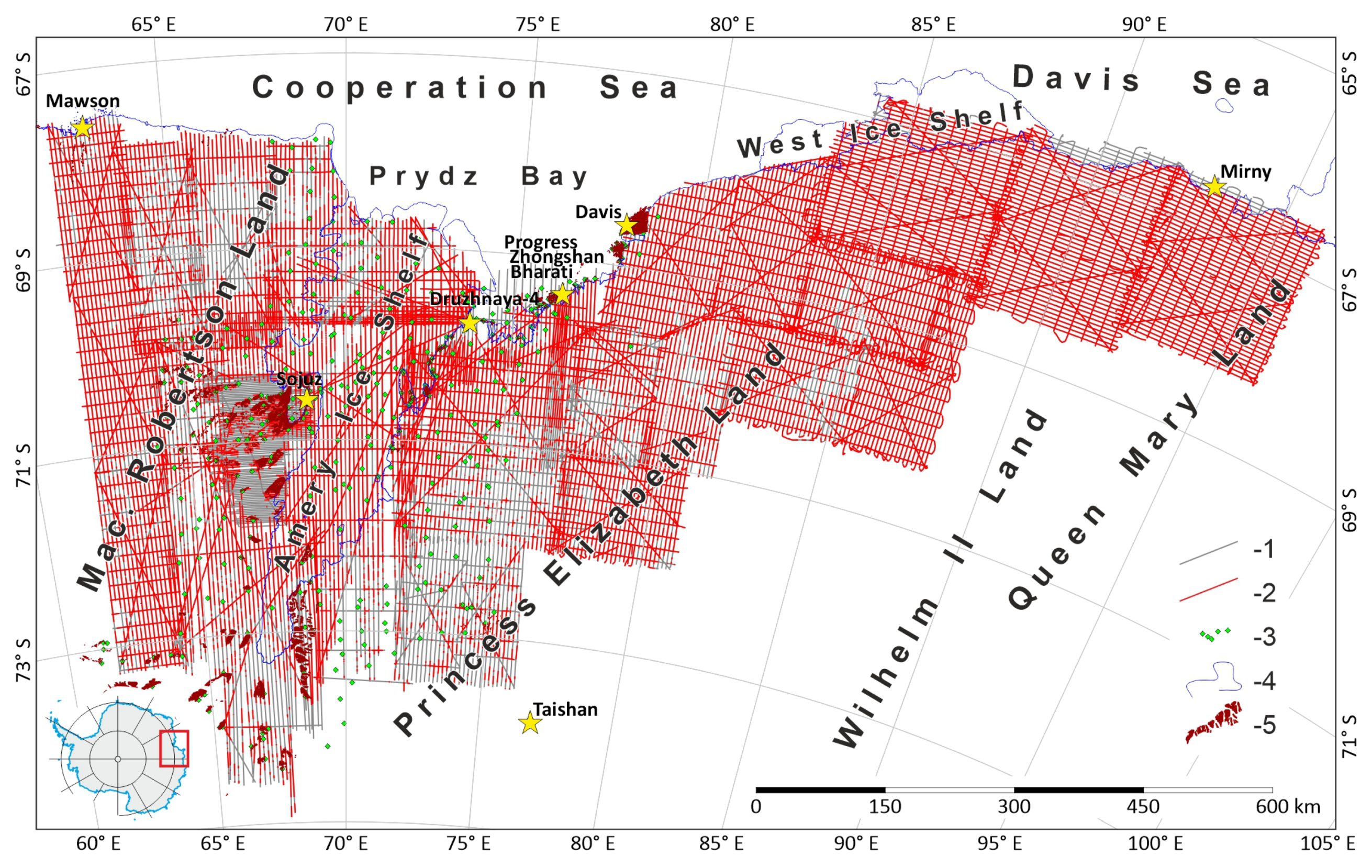
The area of the study spreads for about 1500 km from the Australian Mawson Station (Mac. Robertson Land, East Antarctica) in the west, covering Amery Ice Shelf, Princess Elizabeth Land and Wilhelm II Land to the Shackleton Ice Shelf (Queen Mary Land, East Antarctica) in the east, and from the Antarctic coast in the north, to the inland for some hundred kilometers in the South (Figure 1). It includes the Lambert rift belt, one of the most interesting and important tectonic structures of East Antarctica; fragments of the Prince Charles and Grove mountains; and Amery Ice Shelf.

3. Data and Methods

3.1. Field Studies

The basis of this scientific work is the Russian RES data collected during the systematic airborne geophysical studies of the Soviet Antarctic Expedition (SAE) and Russian Antarctic Expedition (RAE) carried out in the twenty-six Austral summer field seasons of 1985–1988, 1989–1991, 1993–1995, 1999/2000, and 2002–2020; and the seismic reflection soundings which were done in 1971–1974 [12,14]. The airborne geophysical complex includes an ice-penetrating radar system and a magnetometer. The flights are traditionally performed on a network with a distance of 5 km between the standard routes. The only exception was the survey which was done in the field season of 1985/86. It was carried out with a distance between standard routes of 2 km. The total area of all RES surveys is 587 thousand sq. km (Figure 1). An Ilyushin aircraft IL-14 (Figure 2a) was used until 1990, after which time a light Antonov aircraft An-2 (Figure 2b) has been consistently used. In December 1982, before the commencement of airborne geophysical research, on the shore of Beaver Lake (Jetty Oasis, the Prince Charles Mountains), the field base Soyuz was opened, which also served as a base for airplanes and was used for a long time as the logistical support for geological explorations. Subsequently, the field base Druzhnaya-4 (1 January 1987) and Progress Station (1 April 1988) were also opened to additional logistic support for all Russian research in this area. They have been used as the bases for aircraft for more than thirty years. Since 2017, the airstrip of Mirny Station has been used as the home airport.

At the initial stage, in 1985/86, RES studies were carried out by an MPI-300 ice-penetrating radar system with the main frequency of 300 MHz, developed by the PMGRE and the Mari Polytechnic Institute (Russia). This high frequency was chosen because the research of that field season was focused on the almost completely uncovered area of the Else Platform. Then, starting from the 1986/87 field season, the MPI-60 ice-penetrating radar system (the same radar with decreased frequency to 60 MHz) was used because the electromagnetic wave with lower frequencies penetrates the ice deeper. Subsequently, the MPI-60 radar was modernized several times, but not radically. In 2013, a new RLK-130 ice-penetrating radar system with the main frequency of 130 MHz was developed and put into operation, and has been used until now. The technical characteristics of these devices are described in detail in [12,14].

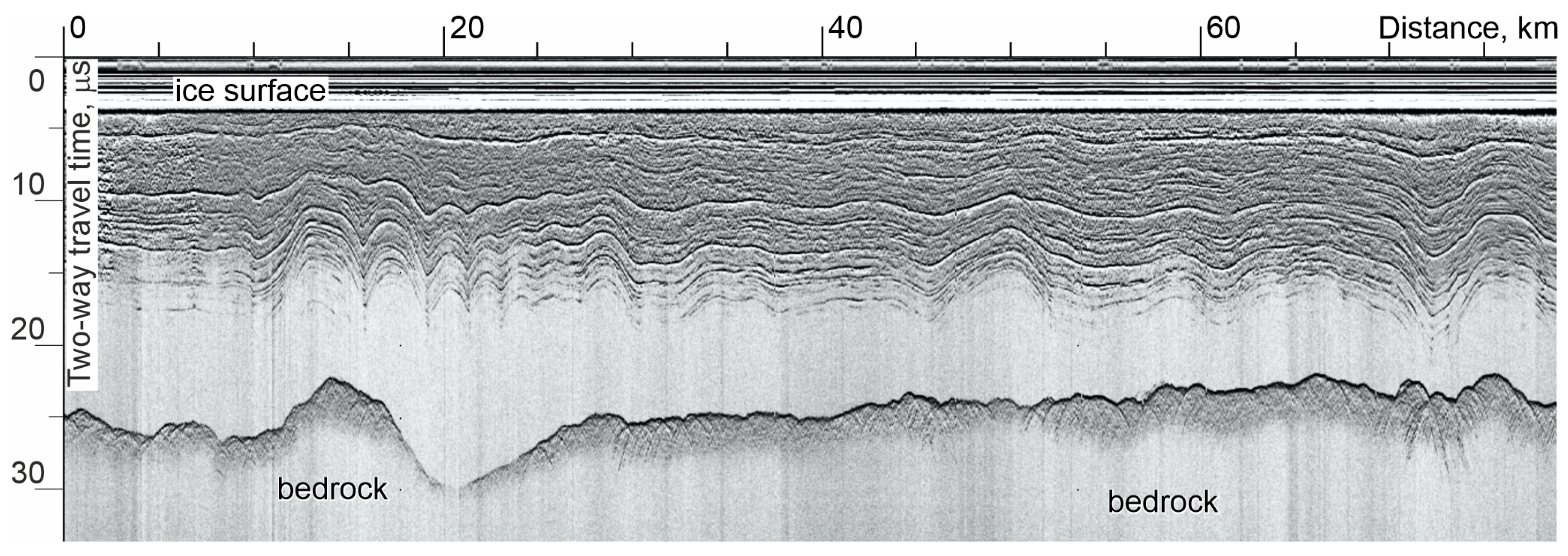
RES data collected in the 1980s and 1990s were registered on 35-mm film. The transition from analogue to digital registration made truly revolutionary changes, since it became possible not only to obtain better data but also to involve computer signal processing, which significantly expanded the scope of the method. The analogue-to-digital converter (ADC), which was used in 1999/2000, had a sampling interval of 140 ns and 6-bit amplitude sampling. Subsequently, its parameters were improved to the recording interval of 80 ns and improved the ADC to 8 bits. The new RLK-130 ice-penetrating radar system has an ADC with 24 bits and 38.46 ns sampling. A detailed technical description can also be found in [12,14]. The radio-echo time-section collected in 2013/14 as an example is shown in Figure 3.

The navigation of the plane during the research of 1985–87 was carried out using aerial photography and the Doppler method. The standard navigation equipment DISS-013 and the aviation gyrocompass GPK-2 were used for it. Aerial photography was performed using the AFA-TE 55 aerial camera. The obtained photographs helped to build preliminary compilations in which natural landmarks were marked. In the areas poor of natural landmarks, additional ones were set. Their coordinates were determined astronomically by the Sumner method. The altitude of the flight was determined by the RV-18 radio altimeter, and the absolute height was measured by barometric method, using the BS-6 string barometer. The navigational horizontal accuracy of that research varied from 175 to 750 m, depending on the number of landmarks; the flight altitude accuracy was 50 m [12,14]. Since 1989, a satellite navigation system has been used for airborne explorations, which significantly improved the accuracy of the surveys. MX-4400 GPS NAVSTAR receiver was applied in the early research. The navigational accuracy decreased to about 30 m in that time. Starting in 2003, the satellite navigation receivers TNL-1000 and SVeeEight Trimble have been used. They have increased the accuracy up to 13 m [12,14].

To measure the sea depths under Amery Ice Shelf, seismic reflection soundings were carried out in 1971–74 over a 30 × 30 km network. This survey covered the area of about 205 thousand sq. km. (Figure 1). Seismic stations SS-24P and SMP-24 were used in the works. Registration was carried out on C-120 seismic receivers. Acoustic waves were excited by TNT sticks 60 × 60 × 150 mm, put in boreholes to the depth of 2–3.5 m, with snow covering. The amount of charge varied from 0.2 kg to 15 kg, depending on the geological situation. Reflected waves were registered on two orthogonal profiles, each 275 m long, consisting of six geophones located 50 m apart. Somner astronomical navigation was used. The accuracy of the seismic measurements for the sea depth was ±5% [12,14].

3.2. RES Data Processing

RES data collected during the fieldwork in 1985–95 were recorded on film. These materials were digitized on Pericolor-300 scanner (Numelec SA, France). RES data have been recorded digitally since 1999 and were initially generated in a special format. In addition, these files contain profile time, navigation, radio altitude and special markers which are input by hand by the ice radar staff to help future interpretation of the data. These files are converted into SEG-Y format, convenient for subsequent storage and processing. Processing of the RES data included digitizing the ice surface and ice base along the radio-echo time-sections. It delayed the electromagnetic return signal, which propagated into the glacier. The delay multiplied by the half of velocity of electromagnetic wave propagation in the media gives the ice thickness. A uniform velocity of the electromagnetic wave propagation in the glacier equal to 168 m/$\mathsf{\mu }$s was used for time-to-depth conversion [21]. The processing was carried out by different computer programs, e.g., SeisVision system of the GeoGraphix professional seismic data processing package (LMKR Ltd., Calgary, AB, Canada), and also programs developed by ourselves.

All geodetic information was brought to the ellipsoid WGS-84 (the data collected before 1993 were calculated on the ellipsoid Pulkovo-42). All RES data were interconnected, and fragments of profiles corresponding to significant discrepancies were analyzed, referring to the original time sections, and then, if necessary, adjusted. This made it possible to significantly improve the quality of the final map. The cross-over analysis demonstrates the average ice thickness error is about 17 m. The maximum value (just some points) reaches more than 600 m in the Mawson escarpment and some other places of the Lambert Deep. These large differences are because this is an area of large gradients of the bedrock, where we carried out research in the past with non-satellite navigation. The cross-over histogram is depicted in Figure 4.

RES surveys are well-known to have gaps related to the nature of the propagation of the electromagnetic waves in the ice and their reflections from the bedrock. RES profiles with and without reflections from the ice base are depicted in Figure 1. The overall information content of the surveys is 83.6%.

3.3. Compilation of the Ice Thickness Data

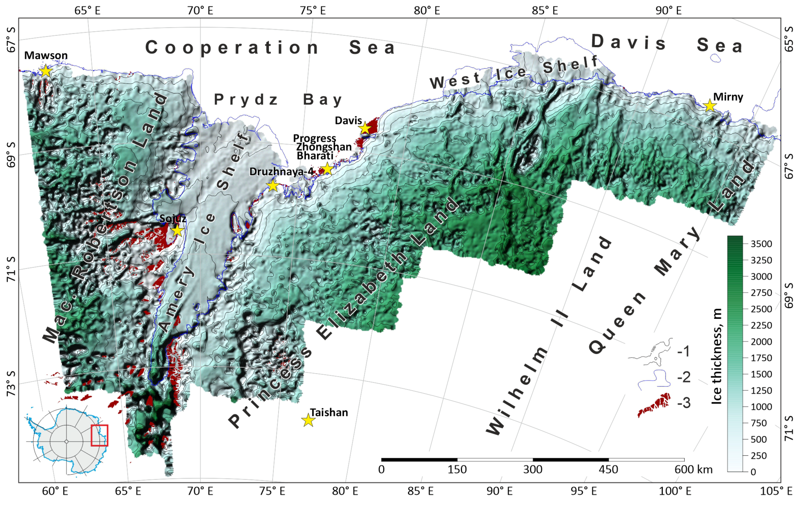
Ice thickness of the research area is shown in Figure 5. It was compiled by gridding of the ice thickness data using the inverse distance method. The distance between the grid nodes is 1 × 1 km. The averaging radius is 7 km with the following minor smoothing and manual adjustment in some places to improve the visual perception. The well-known Surfer 20.2 (Golden Software LLC, Golden, CO, USA) mapping program has been used. As the distance between the standard profiles is about 5 km, the averaging radius of the griding less than 1 km is impractical to consider, because the violation of the inter-profile correlation becomes visually noticeable. Nevertheless, the averaging radius significantly greater than 5 km leads to considerable smoothing of the resulting grids. Thus, the value of 7 km is a compromise option that allowed grid generation of acceptable quality.

The inverse distance method was chosen on the basis of the experience of previous works. The comparative analysis of the results of gridding by various methods: inverse distance, Kriging, and minimum curvature showed that the differences in formal parameters (the average grid error, the shape of the distribution density of random variables) are purely symbolic, but the grids formed by inverse distance are visually perceived as more natural compared with the other ones.

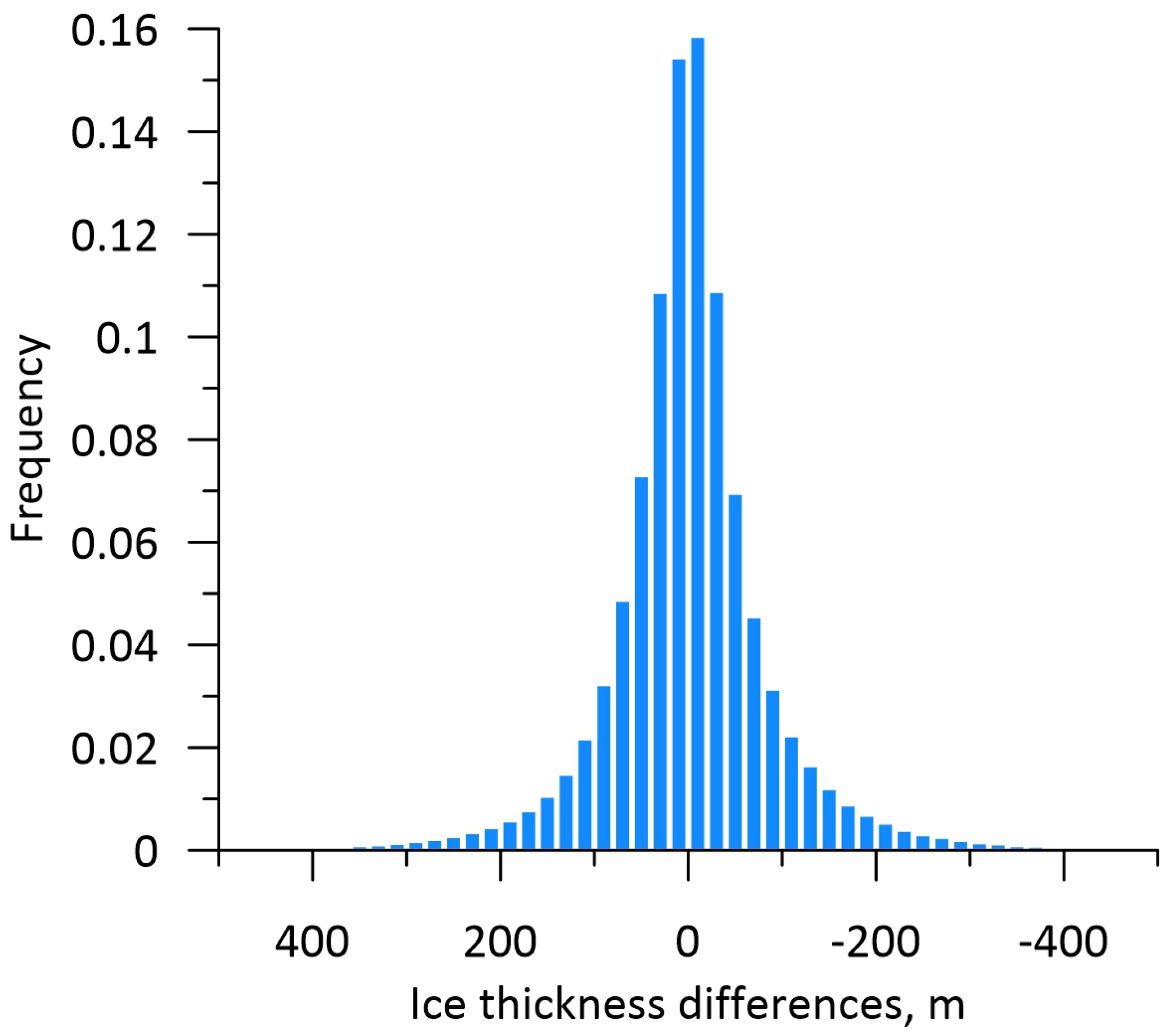
The summary histogram of the ice thickness grid errors (the difference between the data from the grid and the measurements on the profiles) is depicted in Figure 6. It shows that most of the residuals are concentrated in the range of the first tens of meters. Statistical analysis performed on 1,638,861 physical points (it is total value or RES research) shows that the average value of the discrepancy is 0.7 m. This indicates the absence of systematic errors; i.e., in general, the ice thickness grid is sufficiently uniform concerning the measured values, and their total deviation on both sides is generally compensated. The standard deviation is 74 m. This value, taking into account the fact that the data are very diverse, is an indicator of the good quality of the compilation.

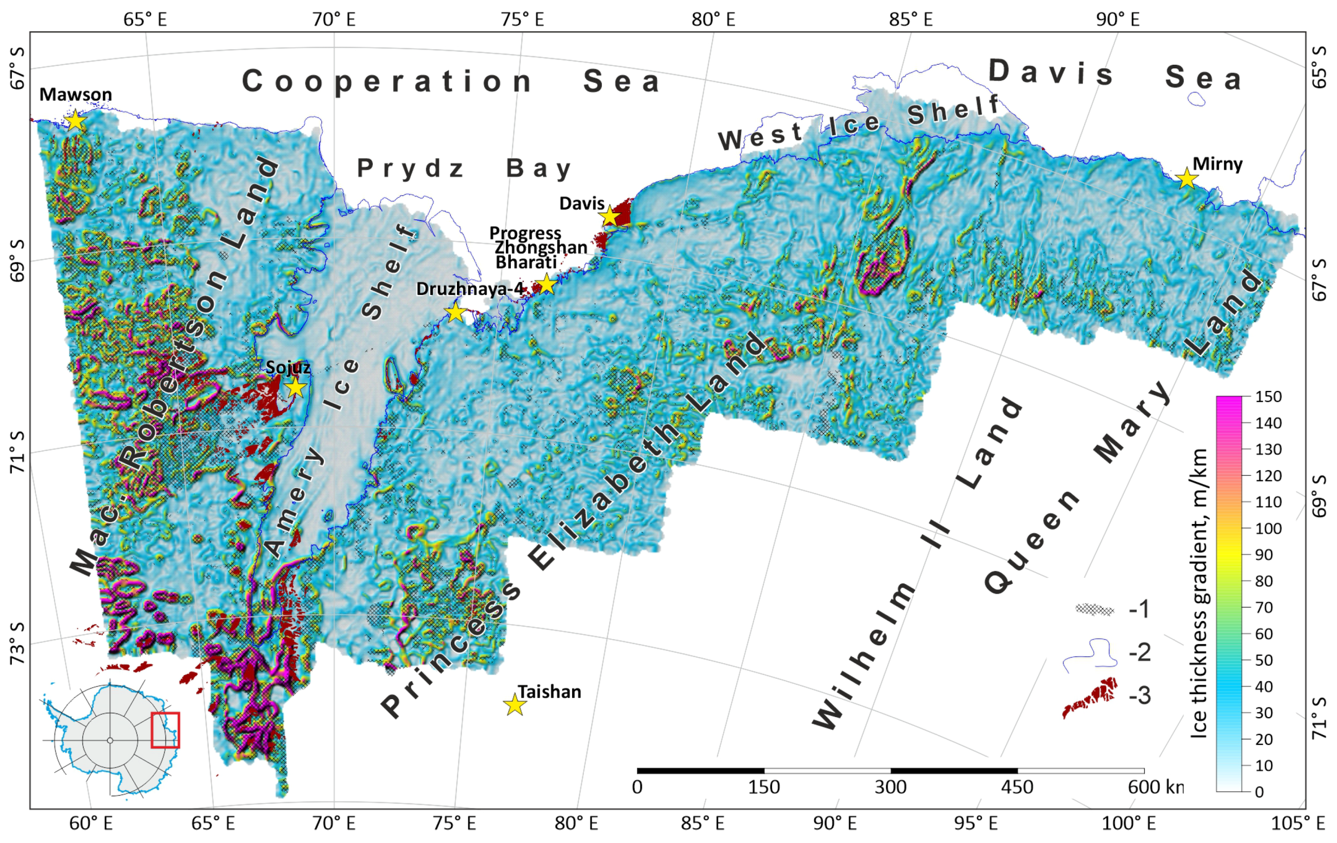
An analysis of the causes of large grid errors is undertaken. The ice thickness gradients (the first derivation of the thickness on the horizontal coordinates) are shown in Figure 7. In the same image, the areas with grid errors of more than 100 m are hatched. This demonstrates that significant errors tend to occur in the areas of high gradients. In general, this is consistent with smoothing error when griding data characterized by significant gradients or variations lead to their smoothing. This leads to an increase in grid error compared with low-gradient areas.

A radio wave propagation velocity of 168 m/$\mathsf{\mu }$s was used for transformations. The choice of this value was based on the results of a review of its measurements in Antarctica [22]. On the other hand, it varies in wide limits from 164 m/$\mathsf{\mu }$s in the Antarctic inland to 174 m/$\mathsf{\mu }$s on the ice shelves, where the relative thickness of the high-velocity snow-firn layer is great [22]. In this sense, the velocity cannot be the same and depends on the ratio of the thickness of the ice and the snow-firn layer. It was well demonstrated in [23]. However, this value is known only for very few regions of Antarctica, where the specialized glaciological studies were carried out. Thus, correction of the electromagnetic velocity in the glacier requires a fairly serious justification and additional specialized work. Due to it, the choice of a certain single effective average velocity for the entire region of generalization is justified.

3.4. Compilation of the Ice Base and Bedrock Topography

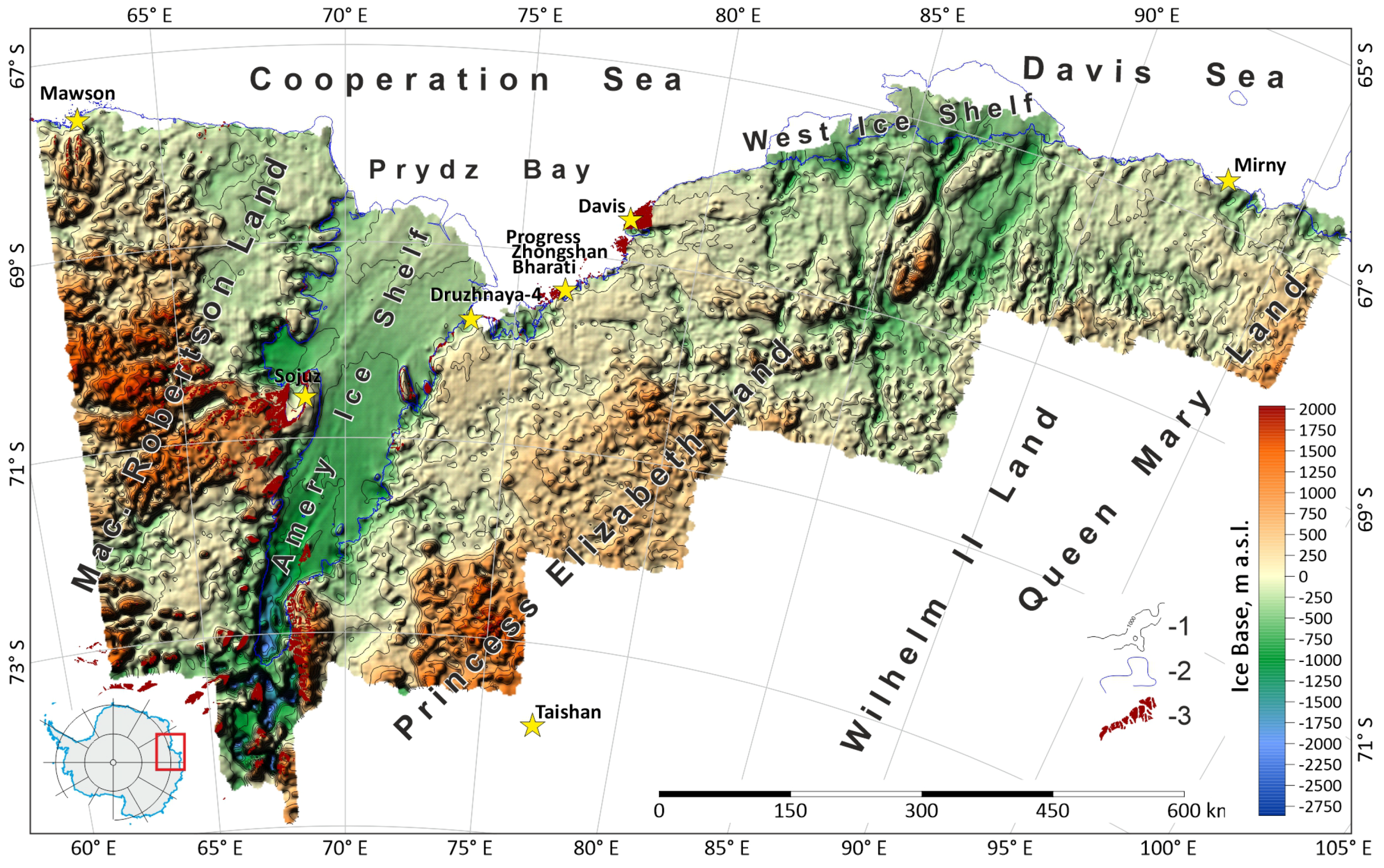
An ice base grid was formed by subtracting the ice thickness grid from the ice surface grid, which was used from the combination of satellite radar and laser altimetry data from Antarctica [24]. It was applied to the compilation of the most modern map of the subglacial relief of Antarctica in the framework of the Bedmap2 International Project [19]. Ice base is depicted in Figure 8.

The difference between the ice base and the bedrock is in taking into account the depths of the World Ocean and subglacial lakes. In our case, its compilation requires generating the grid of the water depths under Amery Ice Shelf and adding to it the depths of the surrounding marine water and a small part of the Southern Ocean. After that, it should be subtracted from the ice base grid on the relevant sites.

The grid of the seawater depths under the Amery Ice Shelf is formed by gridding the reflection seismic data [14]. For this purpose, the inverse distance method of Surfer 20.2 (Golden Software LLC, Golden, CO, USA) was used. It is necessary to note that only 38 measurements are located on the Amery Ice Shelf. They are distributed extremely unevenly. However, in general, it can be considered that the characteristic distance between neighboring measurement points is about 30 km Figure 1. To obtain a bathymetric map of the Amery Ice Shelf area, the distance between the grid nodes was chosen to be 6 km with an averaging radius of 40 km. Then, the resulting grid was masked along the grounding line and ice front.

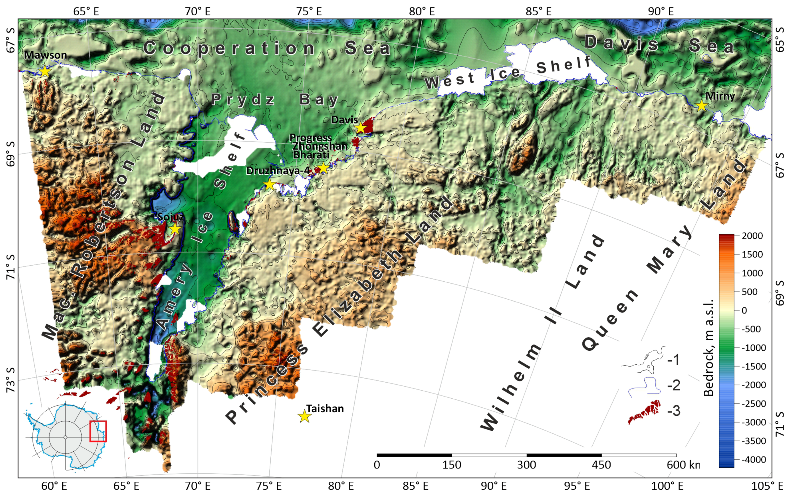
The coastal bathymetry data were obtained from the results of the Bedmap2 project [19], which, in turn, were obtained from the international GEBCO project. Initially, these data are a grid with a distance between nodes 1 × 1 km, i.e., the same parameters as used in our compilation. The latter circumstance greatly simplified the processing. Both bathymetric grids (the marine part and depth under Amery Ice Shelf) were merged. The bedrock topography was compiled by subtracting the depth grid from the ice base grid. The bedrock topography is shown in Figure 9.

4. Results

The main result of this scientific work is preparation of the ice thickness, ice base, and bedrock maps (grids) of the research area.

4.1. Ice Thickness

The thickness of the research area (Figure 5) varies from a few meters in the outcrops areas to 3620 m in the local depressions of the subglacial relief. It increases in the southen direction towards the interior regions of Antarctica. The average thickness is about 1220 m. The total volume of the ice is about 710.5 thousand cubic km, which contains about 6.5 × 10${}^{12}$ tons of freshwater.

This area contains several ice shelves, including the Amery Ice Shelf. Its thickness varies from 150–300 m at the ice front, to 800–900 m at the southwestern grounding line. The Western Ice Shelf is characterized by thicknesses ranging from 150–200 to 300–500 m.

4.2. Subglacial Landscape

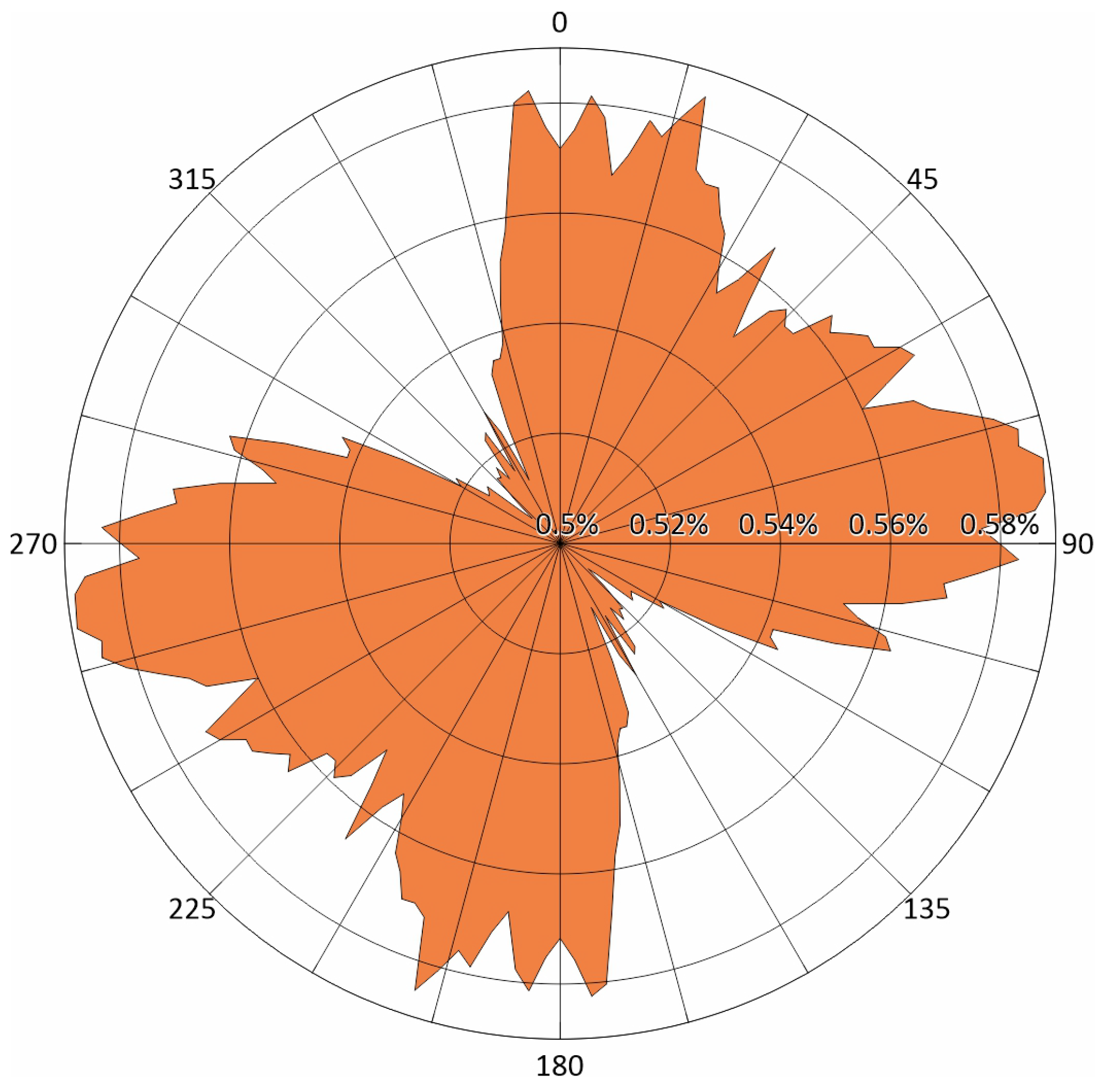
The bedrock heights, including the marine and ocean continuation (Figure 9), vary from −2860 m in the bathyal part to 2040 m in the Grove Mountains area. The dominant morphostructure is the Lambert Rift valley. It determines the structural tectonic plan of the entire region. The rose diagram of the lineaments of the bedrock is depicted in Figure 10. It was plotted automatically with a special computer program. The algorithm was based on the idea that the weight of lineal elements increases with the slope and the number of connected elements (non-published). The rose diagram shows that the main directions of the bedrock orographic forms lie mostly in three intervals: 345${}^{\circ }$–30${}^{\circ }$, 45${}^{\circ }$–70${}^{\circ }$, and 70${}^{\circ }$–100${}^{\circ }$. The first one is associated with the Lambert Rift Valley, and its marine continuation, along with the area toward the subglacial valleys located on Wilhelm II Land, south of the West Ice Shelf, associated with the Gausberg Rift [1]. The second interval reflects the structural tectonic plan of the Prince Charles Mountains located in the eastern and southern parts of Mac. Robertson Land. Finally, the last interval is related to the edge of the continental slope.

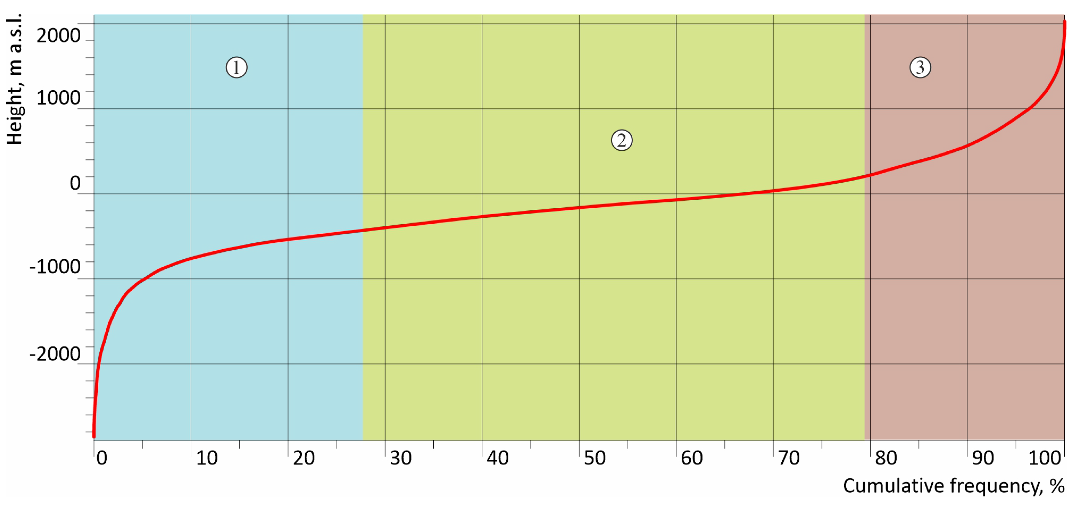
The hypsographic curve of the bedrock topography of the study area is depicted in Figure 11. The most territory occupies lowlands located in the range of heights from about 800 m to 200 m. It is about 70% of the total square of the research area. It includes almost the entire sea shelf, from the coastline to the edge of the continental slope, except for some small basins and canyons. The lowlands also adjoin the Prince Charles and Grove mountains. They are mostly located in the eastern part of Princess Elizabeth Land, Wilhelm II Land, and in the western part of Queen Mary Land. The lowlands located to the west of the Lambert Rift Valley are characterized by the absence of directions of lineaments. The subglacial orographic structures of the lowlands located to the south of the Western Ice Shelf have the submeridional directions.

The next in distribution are hills and low mountains, located in a range of heights from 200 m to the highest measured in this territory (2040 m). They occupy about 22% of the research area (Figure 11). These subglacial orographic structures are mainly located in the eastern and southeastern parts of Mac. Robertson Land (the Prince Charles Mountains) and the south-western part of Princess Elizabeth Land (the Grove Mountains).

Deep-water basins and trenches, located in the range of absolute heights from the minimal volumes (−2860 m) to −800 m, occupy the smallest part (about 8%) of the research area (Figure 11) and cover the deepest part of the Lambert Rift Valley, the continental slope and the bathyal part of the Southern Ocean. In addition, there are separate structures on the shelf of the Cooperation Sea and the Davis Sea.

4.3. Bottom Melting

Thermophysical processes occurring inside the glacier and at its base are critical for understanding the dynamics of the glacier and its evolution. It is the temperature that affects the viscosity of ice, and consequently, its plastic properties [25,26,27]. Herewith, the presence of water or wet soil under the glacier has affects the most the dynamics of the glacier slips, which radically changes the nature of its movement and the distribution of velocities in its thickness [26,28,29,30]. Therefore, identifying areas of bottom melting and assessing the intensity of this process is an important objective of fundamental scientific research in Antarctica. Bottom melting is also the main factor in the formation of subglacial reservoirs (probably, except for the subglacial Lake Vostok, as its genesis may be somewhat different [31,32,33]) by filling negative forms of the subglacial relief with meltwater. According to the heat conduction equation, geothermal heat flux (GHF), which is related to the Earth’s crust structure, is the main factor not only for the bottom melting but also for the entire distribution of temperature in the ice sheet.

The data assembled allow a preliminary estimate of the bottom melting rate. There are many different models of heat transfer in the body of a glacier. The most recent [26,28,29,30,34,35,36] and many others are complicated and take into account ice dynamics too. However, the model of I.A. Zotikov [37], which is a further development of the well-known model of Gordon Robin [25], also can be used for a rough estimation. Zotikov’s model makes it possible to discover the critical glacier thickness $T_{CR}$:

$$T_{CR}=\frac{2\lambda \xi }{{\mathrm{\Lambda }}_G\sqrt{2\pi }}(t_M-t_S){\left[erf\left(\xi \right)\right]}^{-1},\xi \equiv \sqrt{\frac{T{w}_S}{a}},$$

where $\lambda$ = 2.22 W m${}^{-1}$K${}^{-1}$ is the thermal conductivity; a is the thermal diffusivity of ice, a = 1.15 × 10${}^{-6}$ m${}^2$s${}^{-1}$; $t_M$ is the melting temperature, corrected by the ice thickness T; $t_M=-T/1149$ [27]; ${\mathrm{\Lambda }}_G$ is the geothermal heat flux; and $erf\left(z\right)$ is a Gaussian

$$erf\left(z\right)=\frac{2}{\sqrt{\pi }}\underset{0}{\overset{z}{\int }}exp(-x^2)dx.$$

Bottom melting starts when $T_{CR}\ge T$.

The bottom melting rate $w_B$ can be found from solving the equation:

$${\mathrm{\Lambda }}_G=\rho q_F{w}_B+{\mathrm{\Lambda }}_G\frac{T_{CR}}{T}\times \frac{\sqrt{1-n}exp(-0.5c^2{\xi }^2)erf\left(\xi \right)}{erf\left(\xi \left[c+\sqrt{1-n}\right]\right)-erf\left(c\xi \right)},$$

(1)

where

$$n\equiv \frac{w_B}{w_S},c\equiv \frac{n}{\sqrt{1-n}}.$$

Ice density $\rho$, $\rho$ = 910 kg m${}^{-3}$.

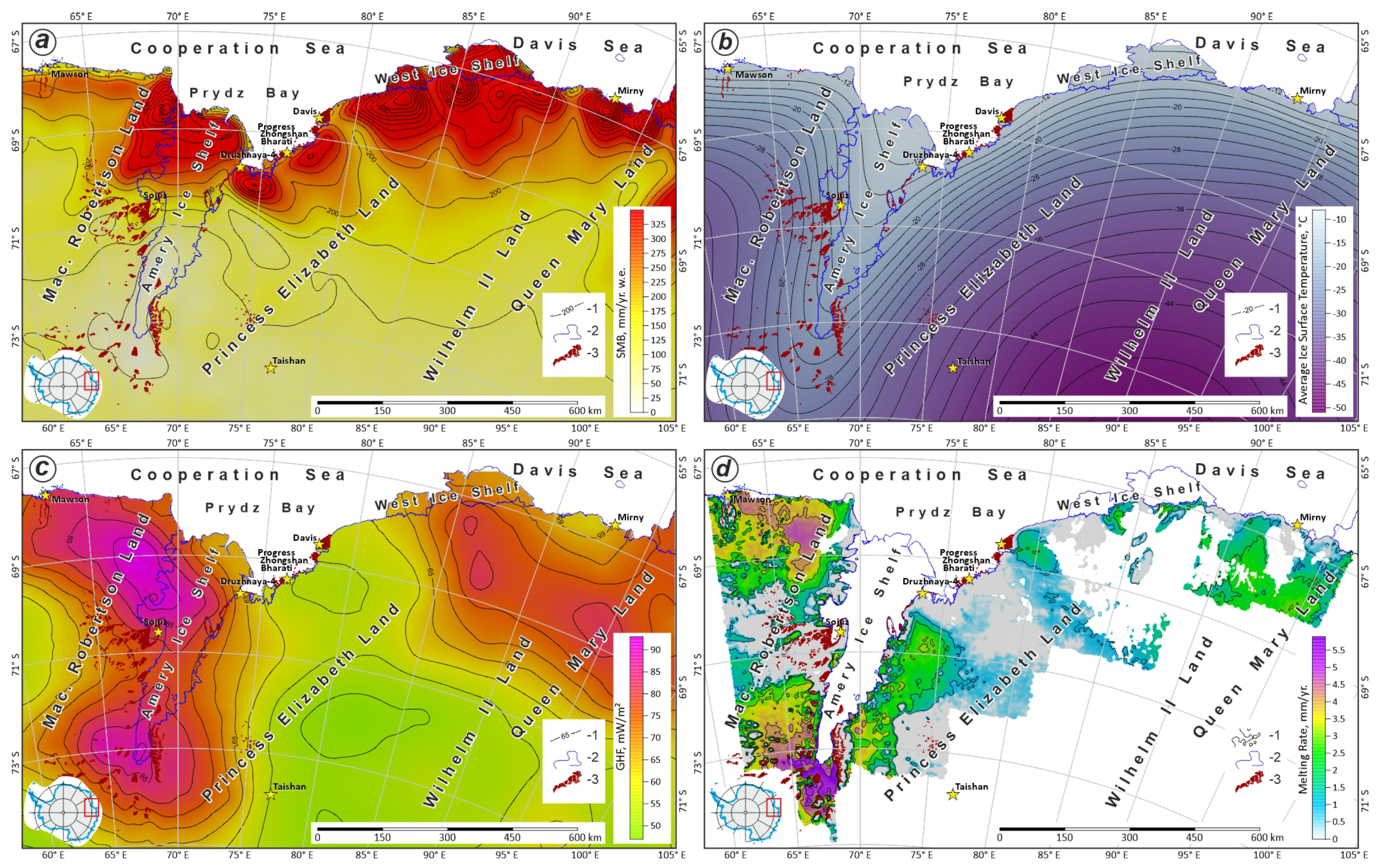
Zotikov’s model is most robust where ice velocity is relatively low, and hence frictional heating is minimal. It is an estimate that should be used to improve models to get more precise results. The melting rate was calculated from Equation (1) by standard numerical methods. Accumulation rate (SMB) required for this model was taken from [38], and it is depicted in Figure 12a. Ice surface temperature, also required, was from the Russian Atlas of Antarctica [39]. It is shown in Figure 12b. Geothermal heat flux was taken from [40] and it is depicted in Figure 12c. Finally, the computed bottom melting rates are depicted in Figure 12d.

The modeling shows that the bottom melting rate occupies most of the bedrock covered by ice. The maximum melting rate (5.7 mm/yr) is rich in the southern part of the Lambert Deep and related to the Lambert rift belt [1]. The total annual basal melting is about 0.633 cubic kilometers for the area of 316.3 thousand sq. km. It is about 54% of the total area of our airborne survey. Bottom freezing occupies about 100.1 thousand sq. km. of the area, and 166.5 thousand sq. km could not be defined in the framework of the considered model. The bottom freezing and low melting rate areas are related to the Prince Charles Mountains, Grove Mountains, and lowland of the western part of Princess Elizabeth Land. The average annual melting rate is about 2 mm/yr.

5. Discussion

The ice thickness, subglacial, and bedrock topography maps discussed above are more accurate and detailed today than ever. That is related to several aspects. For the last two decades, airborne scientific research has been carried out with modern equipment, which has high accuracy. For logistical reasons, the area covered by these surveys was represented as a gap on the map of Antarctica. Hence, our research has been an important and significant addition to the database of the international projects Bedmap [18] and Bedmap2 [19], where our data were gradually added as the work progressed. They have also been included in the database of the next generation of these projects, Bedmap3. These results will be presented in the near future. It should be noted that our studies were carried out systematically on a regular network—the parameters of which (the distance between profiles), and other methodological details of collecting data, have remained unchanged for over 35 years. This is also an additional advantage for the quality of the compiled maps presented in this article and in the Bedmap, Bedmap2, and Bedmap3 projects.

More detailed and accurate maps of the ice thickness that were compiled allow one to obtain more reliable estimates of freshwater reserves, glacioisostatic processes, changes of coastline, and other characteristics/parameters. The presented maps, as well as the initial profile data and RES time-sections, which reflect the structure of the ice sheet, are the basis for a deep geomorphological study of the subglacial relief, and an evolution of the ice sheet based on mathematical modeling. The initial rough estimates of the bottom melting rate were also presented in this article. They show that bottom melting occurs in about a half of the survey area. This is a significantly different finding from the previous results obtained using the same model [33,37]. These new data will certainly improve the results of the modeling using more recent models, e.g., [26,28,29,30].

6. Conclusions and Outlook

The main task of this scientific work was characterizing Russian RES data collected for the last thirty-five years in the coastal part of East Antarctica, discussing the errors, and presenting the set of compiled maps, including ice thickness, ice base, and bedrock topography. They are the basis for future multidisciplinary research, including tectonic and geomorphological reconstructions and mathematical modeling of the subglacial hydrological processes. An initial contribution toward this was presented through basic basal melting estimates via the model of I.A. Zotikov [37]. Future improvements of such can utilize specific multiple alternate models, as suggested.

The results described in this scientific work are the Russian input to the international projects Bedmap, Bedmap2, and active Bedmap3. This amp set is the basis for tectonic and geomorphological compilations and the mathematical modeling.

References

- Golynsky, D.; Golynsky, A. East Antarctic Rift Systems—Key to understanding of Gondwana break-up. Reg. Geol. Metallog. 2012, 52, 58–72. [Google Scholar]
- Kotlyakov, V.M.; Glazovsky, A.F.; Moskalevsky, M.Y. Dynamics of the ice mass in Antarctica in the time of warming. Ice Snow 2017, 57, 149–169. [Google Scholar] [CrossRef] [Green Version]
- Meunier, T.; Williams, R.; Ferrigno, J. US Geological Survey Scientific Activities in the Exploration of Antarctica: Introduction to Antarctica (Including USGS Field Personnel, 1946–59); Technical Report; US Geological Survey: Reston, VA, USA, 2007.
- Mather, K.; Goodspeed, M. Australian Antarctic ice thickness measurements and sastrugi observations, Mac-Robertson Land. Polar Rec. 1959, 9, 436–445. [Google Scholar] [CrossRef]
- Fowler, K.F. Ice Thickness Measurements in Mac. Robertson Land, 1957–1959; ANARE Scientific Report; Bureau of Mineral Resources, Geology and Geophysics: Melbourne, Australia, 1971. [Google Scholar]
- Crohn, P.W. A Contribution to the Geology and Glaciology of the Western Part of Australian Antarctic Territory; Number 52; Antarctic Division, Department of External Affairs: Melbourne, Australia, 1959; p. 103. [Google Scholar]
- Morgan, V.I.; Budd, W.F. Radio-echo sounding of the Lambert Glacier basin. J. Glaciol. 1975, 15, 103–111. [Google Scholar] [CrossRef] [Green Version]
- Allison, I.; Frew, R.; Knight, I. Bedrock and ice surface topography of the coastal regions of Antarctica between 48°E and 64°E. Polar Rec. 1982, 21, 241–252. [Google Scholar] [CrossRef]
- Higham, M.; Reynolds, M.; Brocklesby, A.; Allison, I. Ice radar digital recording, data processing and results from the Lambert Glacier basin traverses. Terra Antart. 1995, 2, 23–32. [Google Scholar]
- Damm, V. A subglacial topographic model of the southern drainage area of the Lambert Glacier/Amery Ice Shelf system—Results of an airborne ice thickness survey south of the Prince Charles Mountains. Terra Antart. 2007, 14, 85–94. [Google Scholar]
- Cui, X.; Greenbaum, J.S.; Beem, L.H.; Guo, J.; Ng, G.; Li, L.; Blankenship, D.; Sun, B. The first fixed-wing aircraft for Chinese Antarctic Expeditions: Airframe, modifications, scientific snstrumentation and applications. J. Environ. Eng. Geophys. 2018, 23, 1–13. [Google Scholar] [CrossRef]
- Popov, S.; Kiselev, A. Russian airborne geophysical investigations of Mac. Robertson, Princess Elizabeth and Wilhelm II Lands, East Antarctica. Earths Cryosphere 2018, XXII, 3–12. [Google Scholar] [CrossRef]
- Cui, X.; Jeofry, H.; Greenbaum, J.S.; Guo, J.; Li, L.; Lindzey, L.E.; Habbal, F.A.; Wei, W.; Young, D.A.; Ross, N.; et al. Bed topography of Princess Elizabeth Land in East Antarctica. Earth Syst. Sci. Data 2020, 12, 2765–2774. [Google Scholar] [CrossRef]
- Popov, S. Fifty-five years of Russian radio-echo sounding investigations in Antarctica. Ann. Glaciol. 2020, 61, 14–24. [Google Scholar] [CrossRef] [Green Version]
- Bo, S.; Siegert, M.J.; Mudd, S.M.; Sugden, D.; Fujita, S.; Cui, X.; Jiang, Y.; Tang, X.; Li, Y. The Gamburtsev mountains and the origin and early evolution of the Antarctic Ice Sheet. Nature 2009, 459, 690–693. [Google Scholar] [CrossRef]
- Popov, S.V. Recent Russian remote sensing investigations in Antarctica within the framework of scientific traverses. Adv. Polar Sci. 2015, 26, 113–121. [Google Scholar] [CrossRef]
- Cui, X.; Wang, T.; Sun, B.; Tang, X.; Guo, J. Chinese radioglaciological studies on the Antarctic ice sheet: Progress and prospects. Adv. Polar Sci. 2017, 28, 161–170. [Google Scholar]
- Lythe, M.B.; Vaughan, D.G.; The, B.C. BEDMAP: A new ice thickness and subglacial topographic model of Antarctica. J. Geophys. Res. 2001, 106, 11335–11351. [Google Scholar] [CrossRef] [Green Version]
- Fretwell, P.; Pritchard, H.D.; Vaughan, D.G.; Bamber, J.L.; Barrand, N.E.; Bell, R.; Bianchi, C.; Bingham, R.G.; Blankenship, D.D.; Casassa, G.; et al. Bedmap2: Improved ice bed, surface and thickness datasets for Antarctica. Cryosphere 2013, 7, 375–393. [Google Scholar] [CrossRef] [Green Version]
- ADD. Antarctic Digital Database, Version 7.0; Scientific Committee on Antarctic Research, British Antarctic Survey: Cambridge, UK, 2016. [Google Scholar]
- Bogorodskiy, V.V.; Bentley, C.R.; Gudmandsen, P.E. Radioglaciology; Reidel Publishing Company: Dordrecht, The Netherlands, 1985; p. 254. [Google Scholar]
- Popov, S.V.; Sheremet’yev, A.N.; Masolov, V.N.; Lukin, V.V.; Mironov, A.V.; Luchininov, V.S. Velocity of radio-wave propagation in ice at Vostok station, Antarctica. J. Glaciol. 2003, 49, 179–183. [Google Scholar] [CrossRef] [Green Version]
- Rees, W.G.; Donovan, R.E. Refraction correction for radio-echo sounding of large ice masses. J. Glaciol. 1992, 38, 302–308. [Google Scholar] [CrossRef] [Green Version]
- Bamber, J.L.; Griggs, J.A. A new 1 km digital elevation model of the Antarctic derived from combined satellite radar and laser data—Part 1: Data and methods. Cryosphere 2009, 3, 101–111. [Google Scholar] [CrossRef] [Green Version]
- Robin, G. Ice movement and temperature distribution in glaciers and ice sheets. J. Glaciol. 1955, 2, 523–532. [Google Scholar] [CrossRef] [Green Version]
- Greve, R.; Blatter, H. Dynamics of Ice Sheets and Glaciers; Springer Science & Business Media: Berlin/Heidelberg, Germany, 2009; p. 300. [Google Scholar]
- Paterson, W. The Physics of Glaciers; Rutterworth Hinemann: Oxford, UK, 1994; p. 496. [Google Scholar]
- Huybrechts, P. The Antarctic Ice Sheet and Environmental Change: A Three-Dimensional Modelling Study. Ber. Polarforsch. 1992, 99, 241. [Google Scholar]
- Greve, R. A continuum–mechanical formulation for shallow polythermal ice sheets. Philos. Trans. R. Soc. Lond. Ser. Math. Phys. Eng. Sci. 1997, 355, 921–974. [Google Scholar] [CrossRef] [Green Version]
- Pattyn, F. A new three-dimensional higher-order thermomechanical ice sheet model: Basic sensitivity, ice stream development, and ice flow across subglacial lakes. J. Geophys. Res. 2003, 108, 2382. [Google Scholar] [CrossRef]
- Leitchenkov, G.; Belyatsky, B.; Popkov, A.; Popov, S. Geological nature of subglacial Lake Vostok. Data Glaciol. Stud. 2005, 98, 81–91. [Google Scholar]
- Siegert, M.J. Reviewing the origin of subglacial Lake Vostok and its sensitivity to ice sheet changes. Prog. Phys. Geogr. Earth Environ. 2005, 29, 156–170. [Google Scholar] [CrossRef]
- Zotikov, I. The Antarctic Subglacial Lake Vostok; Springer Praxis Books; Springer: Berlin/Heidelberg, Germany, 2006; p. 139. [Google Scholar] [CrossRef]
- Fürst, J.J.; Rybak, O.; Goelzer, H.; De Smedt, B.; de Groen, P.; Huybrechts, P. Improved convergence and stability properties in a three-dimensional higher-order ice sheet model. Geosci. Model Dev. 2011, 4, 1133–1149. [Google Scholar] [CrossRef] [Green Version]
- Maris, M.N.A.; de Boer, B.; Ligtenberg, S.R.M.; Crucifix, M.; van de Berg, W.J.; Oerlemans, J. Modelling the evolution of the Antarctic ice sheet since the last interglacial. Cryosphere 2014, 8, 1347–1360. [Google Scholar] [CrossRef] [Green Version]
- Lösing, M.; Ebbing, J.; Szwillus, W. Geothermal heat flux in Antarctica: Assessing models and observations by Bayesian inversion. Front. Earth Sci. 2020, 8. [Google Scholar] [CrossRef] [Green Version]
- Zotikov, I. Bottom melting in the central zone of the ice shield on the Antarctic continent and its influence upon the present balance of the ice mass. Hydrol. Sci. J. 1963, 8, 36–44. [Google Scholar] [CrossRef]
- van Wessem, J.M.; van de Berg, W.J.; Noël, B.P.Y.; van Meijgaard, E.; Amory, C.; Birnbaum, G.; Jakobs, C.L.; Krüger, K.; Lenaerts, J.T.M.; Lhermitte, S.; et al. Modelling the climate and surface mass balance of polar ice sheets using RACMO2— Part 2: Antarctica (1979–2016). Cryosphere 2018, 12, 1479–1498. [Google Scholar] [CrossRef] [Green Version]
- Kuroedov, V. Atlas of the Oceans, Antarctica; Glavnoe Upravlenie Navigatsii i Okeanografii Min. Oborony RF: St. Petersburg, Russia, 2005; p. 280. [Google Scholar]
- Martos, Y.M.; Catalán, M.; Jordan, T.A.; Golynsky, A.; Golynsky, D.; Eagles, G.; Vaughan, D.G. Heat flux distribution of Antarctica unveiled. Geophys. Res. Lett. 2017, 44, 11417–11426. [Google Scholar] [CrossRef] [Green Version]
Figure 1.
Locations of airborne RES and seismic reflection soundings. 1—Airborne RES flights; 2—portions of RES flights with reflection from the ice base; 3—seismic reflection soundings; 4—ice front and grounding line from [20]; 5—outcrops from [20].
Figure 2.
Russian (Soviet) survey airplanes: (a) Ilyushin aircraft IL-14 and (b) Antonov aircraft An-2. Photos from the PMGE collection.
Figure 3.
Radio-echo time-section along the flight line 59008 (2013/14).
Figure 4.
Histogram of the ice thickness errors in the cross-overs of the RES profile.
Figure 5.
Ice thickness of the research area. 1—Ice thickness contours in meters; contour interval is 250 m; 2—ice front and grounding line from [20]; 3—outcrops from [20].
Figure 6.
Histogram of difference between ice thickness grid and line RES data.
Figure 7.
Ice thickness gradients of the research area. 1—areas with grid errors greater than 75 m; 2—ice front and grounding line from [20]; 3—outcrops from [20].
Figure 8.
Ice base of the research area. 1—Ice base contours in meters; contour interval is 250 m; 2—ice front and grounding line from [20]; 3—outcrops from [20].
Figure 9.
Bedrock topography of the research area. 1—Ice base contours in meters; contour interval is 250 m; 2—ice front and grounding line from [20]; 3—outcrops from [20].
Figure 10.
Rose diagram of the bedrock of the research area.
Figure 11.
The hypsographic curve of the research area. 1—Deep-water basins and trenches; 2—lowlands; 3—hills and low mountains.
Publisher’s Note: MDPI stays neutral with regard to jurisdictional claims in published maps and institutional affiliations. |
© 2022 by the author. Licensee MDPI, Basel, Switzerland. This article is an open access article distributed under the terms and conditions of the Creative Commons Attribution (CC BY) license (https://creativecommons.org/licenses/by/4.0/).
Share and Cite
MDPI and ACS Style
Popov, S. Ice Cover, Subglacial Landscape, and Estimation of Bottom Melting of Mac. Robertson, Princess Elizabeth, Wilhelm II, and Western Queen Mary Lands, East Antarctica. Remote Sens. 2022, 14, 241. https://doi.org/10.3390/rs14010241
AMA Style
Popov S. Ice Cover, Subglacial Landscape, and Estimation of Bottom Melting of Mac. Robertson, Princess Elizabeth, Wilhelm II, and Western Queen Mary Lands, East Antarctica. Remote Sensing. 2022; 14(1):241. https://doi.org/10.3390/rs14010241
Chicago/Turabian StylePopov, Sergey. 2022. "Ice Cover, Subglacial Landscape, and Estimation of Bottom Melting of Mac. Robertson, Princess Elizabeth, Wilhelm II, and Western Queen Mary Lands, East Antarctica" Remote Sensing 14, no. 1: 241. https://doi.org/10.3390/rs14010241
Note that from the first issue of 2016, this journal uses article numbers instead of page numbers. See further details here.