
MCMS-STM: An Extension of Support Tensor Machine for Multiclass Multiscale Object Recognition in Remote Sensing Images

School of Electronics and Information Engineering, Harbin Institute of Technology, Harbin 150001, China
*
Author to whom correspondence should be addressed.
Remote Sens. 2022, 14(1), 196; https://doi.org/10.3390/rs14010196
Submission received: 24 November 2021
/
Revised: 30 December 2021
/
Accepted: 30 December 2021
/
Published: 2 January 2022
(This article belongs to the Special Issue Object-Level Remote Sensing Image Information Extraction and Applications)
Abstract
:The support tensor machine (STM) extended from support vector machine (SVM) can maintain the inherent information of remote sensing image (RSI) represented as tensor and obtain effective recognition results using a few training samples. However, the conventional STM is binary and fails to handle multiclass classification directly. In addition, the existing STMs cannot process objects with different sizes represented as multiscale tensors and have to resize object slices to a fixed size, causing excessive background interferences or loss of object’s scale information. Therefore, the multiclass multiscale support tensor machine (MCMS-STM) is proposed to recognize effectively multiclass objects with different sizes in RSIs. To achieve multiclass classification, by embedding one-versus-rest and one-versus-one mechanisms, multiple hyperplanes described by rank-R tensors are built simultaneously instead of single hyperplane described by rank-1 tensor in STM to separate input with different classes. To handle multiscale objects, multiple slices of different sizes are extracted to cover the object with an unknown class and expressed as multiscale tensors. Then, M-dimensional hyperplanes are established to project the input of multiscale tensors into class space. To ensure an efficient training of MCMS-STM, a decomposition algorithm is presented to break the complex dual problem of MCMS-STM into a series of analytic sub-optimizations. Using publicly available RSIs, the experimental results demonstrate that the MCMS-STM achieves 89.5% and 91.4% accuracy for classifying airplanes and ships with different classes and sizes, which outperforms typical SVM and STM methods.
1. Introduction
The diverse types and sizes of objects bring a challenge to object recognition in remote sensing images (RSIs). Recently, mainly owing to its powerful feature abstraction ability, various deep learning technologies have achieved impressive success in different object recognition tasks, such as Fast R-CNN [1], Faster R-CNN [2], local attention based CNN [3], CNN [4], SSD [5] and YOLO [6]. In addition to object recognition, deep learning-based methods are widely used for a wide variety of classification tasks based on remote sensing data acquired by different sensors, such as graph convolution neural networks [7] based hyperspectral image classification [8], and multimodal deep learning-based multisource image classification [9]. Despite the recent advances, deep learning-based methods rely heavily on massive available labeled samples. In comparison, the machine learning-based object recognition method can obtain effective results using a small number of samples.
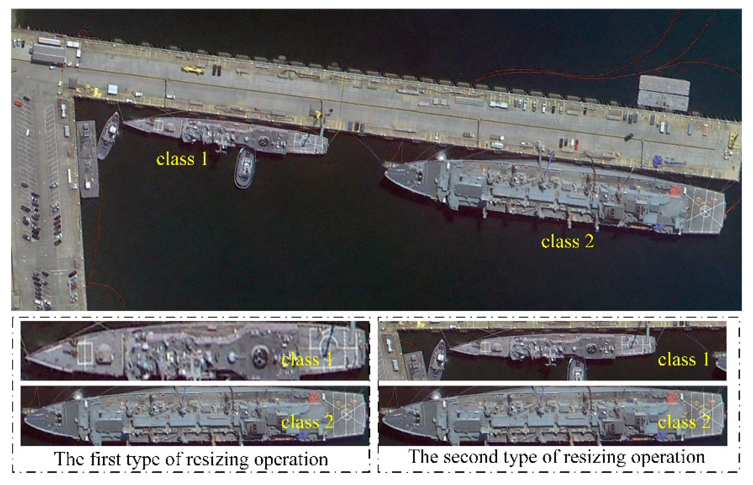
For the object recognition in RSIs, the general procedure consists of two steps, i.e., extracting an object slice using object detection method and recognizing the type of object contained in the slice using a trained classifier. By virtue of the object detection methods, e.g., region proposal-based methods [10,11,12] and saliency-based methods [13,14,15,16], the positions of objects in RSIs can be obtained. Then, the slice of the object can be extracted for subsequent classification. It is worth noting that most existing classifiers, including deep learning methods [1,2,3,4,5] and machine learning methods [17,18,19,20], can only deal with the input of the fixed size. Thereby, two image resizing operations are always used to extract slices containing objects with the fixed size, as shown in Figure 1, one of which extracts the slices by the appropriate size to ensure that the object can be exactly covered, and then resizes the slice to the same size using the image interpolation method [10,11,12]. Another way is to extract slices according to the maximum size of objects to cover each size of object [13,14,15,16]. After obtaining the slices with the fixed size, a proper classifier should be designed to predict the corresponding class label. Among the various machine learning based classifiers, the support vector machine (SVM) as well as its tensor extension, i.e., support tensor machine (STM), are the most worth considering due to a sound theoretical foundation and excellent generality capability. Besides the standard SVM (i.e., ) [17], various variants of SVM were established to improve the performance of SVM from different perspectives, including [18], least-square SVM [19], etc. Since the standard SVM can be considered as a bi-category classifier and thus cannot be used to address multiclass classifications directly, the One-Versus-One (OVO) [20], Error Correcting Output Codes (ECOC) [21], and One-Versus-Rest (OVR) [22] strategies were employed in order to use various binary SVMs to achieve multiclass classifications indirectly. Different from the classic SVM that relies on auxiliary strategies to achieve multiclass classification, the multiclass SVM was developed to classify multiclass objects by solving parameters of multiple classification hyperplanes simultaneously [22]. Besides, based on the multiclass classification mechanism of [22], some other multiclass-oriented SVM variants were developed, e.g., the graph embedded multiclass SVM [23] and the least-squares twin multiclass SVM [24].
Since the object slice can be represented naturally as a tensor in RSI, the tensor-based classifier, i.e., STM, was developed to exploit the structural information embedded in RSI better. According to the supervised tensor learning framework [25] established in 2005, the and were extended to and by applying multilinear operator of tensor space, respectively. Besides, a large number of variants of STMs were established to deal with different classification tasks, such as linear support higher-order tensor machine (SHTM) [26], multi-kernel STM [27], higher rank support tensor machine [28], and support tucker machine [29]. Moreover, the support multimode tensor machine (SMTM) [30] was built to exploit the multimode product of tensor to obtain the results of the multiclass classification for different perspectives, while its multiclass classification strategy is similar to conventional ECOC strategy.
For classifying objects with multiple classes and different sizes, most existing STM methods need to exploit OVO or OVR strategies to train a series of binary classifiers to perform multiclass classification indirectly. The OVO and OVR strategies inherently assume that multiclass classifications can be solved by multiple independent bi-category classifications, ignoring the correlation between multiple classes [23]. Although there exist a few SVM methods that can handle multiclass classification directly, e.g., multiclass SVM [22] and its variants [23,24], their multiclass classification mechanism that is similar to OVR may generate excessive constraints to limit the classification hyperplane, leading to the increase of complexity for training classifier [31]. On the other hand, since the existing STMs only accept tensors with a fixed size as input, it needs to resize the object slices of different classes in RSIs into a fixed size. Considering that objects with different classes usually present different sizes, the typical two resizing operations will bring adverse effect on object recognition, of which the first type of resizing operation will lead to the loss of objects’ scale information, and the second type of resizing operation is easy to cause the slice to contain more background interferences. The examples of two types of resizing operations are given in Figure 1. It is seen that using the second type of resizing operation will lose the scale information of the ships and thus cannot identify ships according to their size feature, and using the first type of resizing operation will generate slices with a large size so that the slice containing ship with class 1 covers excessive background interferences. To deal with the slices to be classified present different sizes, the deep learning method, i.e., the scale free convolution neural network, is built to utilize the global average pooling to map feature maps to unify size [32]. However, for representative machine learning methods, e.g., STM, there is no related work that can process the input slices with different sizes. In comparison to image resizing, the objects with different sizes should be contained by slices with proper sizes to reduce the impact of background interferences and maintain inherent scale information of the contained object, and these slices can be naturally represented as tensors with different dimensions, denoted as multiscale tensors in this paper, while the existing STMs can only process tensor with the same size and cannot process the slices with different sizes represented as multiscale tensors.
Motived by the abovementioned issues, the multiclass multiscale support tensor machine (MCMS-STM) is proposed in this paper. To deal with mutliclass classification, by integrating OVR and OVO strategies to optimization problems, a new multiclass classification mechanism is constructed to use multiple hyperplanes defined by rank-R tensors instead of a single hyperplane defined by rank-1 tensor of STM, where each hyperplane is needed to separate samples with specific classes. Furthermore, to classify objects with different sizes, according to positions of objects obtained from detection results, it is necessary to extract the objects slices with proper sizes rather than the fixed size to reduce the impact of background interferences and maintain inherent scale information of the contained object. These slices with different sizes can be naturally represented as tensors with different dimensions, denoted as multiscale tensors in this paper. Note that the existing STM methods can only process tensor with the same size and cannot process the slices with different sizes represented as multiscale tensors. To deal with input of multiscale tensors, instead of the fixed-dimensional hyperplane used in STM, the M-dimensional hyperplanes are built to separate input of multiscale tensors, and the resulting projecting value is used to predict the class label of input to achieve cross-scale object recognition. In addition, to train the OVO version of MCMS-STM efficiently, a decomposition algorithm is proposed to split the dual problem of the MCMS-STM into a series of sub-optimizations to accelerate the training.
The remainder of this paper is organized as follows. Section 2 consists of some preliminaries, such as the basic definitions and notions, the classical SVM and STM methods. In Section 3, the OVR version and OVO version of MCMS-STM and the corresponding solving methods are presented. Then, the decomposition algorithm is constructed to accelerate the training of the OVO version of MCMS-STM, and the relationship between the multiclass classification mechanism used in MCMS-STM and the existing methods is discussed. In Section 4, the experiments are conducted on publicly RSIs to analyze the parameter setting and the impact of image resizing operation and evaluate the performance of the MCMS-STM. Our conclusion is given in Section 5.
2. Preliminaries and Related Work
Before presenting the MCMS-STM, the notations, abbreviations, the basic tensor algebra used throughout this paper, and the traditional SVM and STM are introduced briefly as follows.
2.1. Notations, Abbreviations, and Tensor Operation
Tensor is the expansion of vector and matrix to the higher dimension, and tensor algebra, also known as multilinear algebra, is the extension of linear algebra to multiway data. To distinguish between tensors, matrices, and vectors, according to the convention in [33], the used symbols throughout this paper are summarized in Table 1.
Then, we summarize all the notations and abbreviations used throughout this paper in Table 2.
The used basic tensor operations throughout this paper are given as follows.
Definition 1.
Frobenius norm and inner product of tensors: The Frobenius normof a tensoris calculated as
The inner product between tensors , is defined as the sum of the products of their corresponding entries, i.e.,
Definition 2.
Mode-k product of tensor: Given tensorand matrix, the mode-k product betweenand B is denoted as, whose results are tensor, as calculated by Equation (3).
Definition 3.
Outer product: The outer product of M vectors (i.e.,) is denoted as, and the corresponding results are represented as an M-order tensor, whose entry with coordinateis calculated by
2.2. Classical Binary and Multiclass Support Vector Machine
Consider bi-category classification task, given training set containing N samples, i.e., , where and denote the input vector of ith sample and the corresponding label, respectively. SVM aims at learning the parameters of classification hyperplane with the largest classification margin from the training set, which can be drawn using the following optimization problem.
where w, b, and C denote the normal vector for classification hyperplane, the bias, the slacking variable, and the regularization parameter, respectively. To obtain the optimal w, the dual problem can be drawn as follows. The detailed derivation can refer to [17].
where denotes the Lagrangian multiplier. Q is a positive semidefinite matrix, where . After solving the optimal , the can be calculated by Equation (7).
Then, the label of test sample x can be predicted by Equation (8).
where denotes the sign function.
The standard SVM can only deal with the bi-category classification problem, while most practical applications can be regarded as multiclass classification problems. Facing this situation, the multiclass SVM, i.e., an extension of SVM in multiclass classification problems, is established to identify samples with different classes.
Given the training set , where and denote the input vector of the ith sample and the corresponding class label. The multiclass SVM aims at learning M classification hyperplanes simultaneously by solving the following optimization problem.
where , bm and denote the normal orientation of M classification hyperplanes, the mth bias, the slacking variable, respectively. The exact solving method can refer to [22].
According to the resulting and bm, the class label of test sample x can be predicted using the following decision function.
2.3. Support Tensor Machine
To better use the structural information of input data represented as a tensor, the STM is extended from SVM to directly separate input in tensor space.
The given training set containing N samples , where denotes the input tensor and denotes the corresponding label. Compared to SVM that separates input in vector space, the STM utilizes the mode-k product to process input in tensor space. The corresponding optimization problem of STM is given in Equation (11).
where denotes the projection vector along with the jth mode of the input tensor. The denotes the projection tensor used to indicate the orientation of the normal orientation for the classification hyperplane. Since the parameters of STM is the M-order tensor, it is difficult to be solved directly. In this way, the alternating optimization scheme is introduced to solve the above optimization, i.e., optimize each in turn by fixing the rest in the kth iteration, where denotes the index of order to be optimized. The optimization problem in kth iteration is equivalent to that in SVM (see Equation (5)) it can be solved by using SVM solver. After the alternating optimization procedure is terminated, the optimal parameters and b can be utilized to predict the label of the test sample , as shown below.
3. Multiclass Multiscale Support Tensor Machine
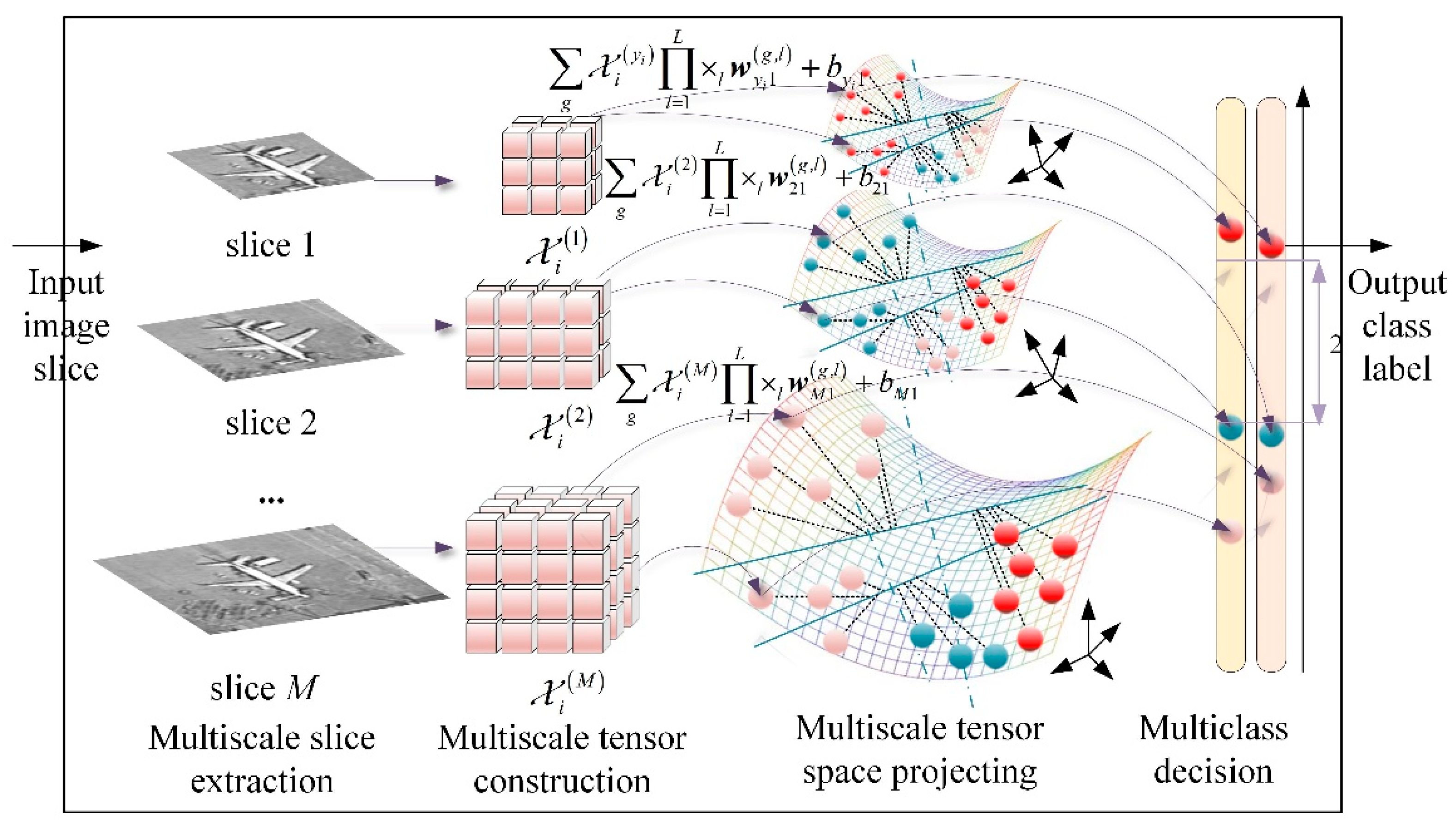
As discussed above, the standard STM fails to deal with multiclass classification, and it requires resizing preprocessing to generate slices of the fixed size to comply with its input requirements, causing loss of scale information or increase of background interferences. To address multiclass multiscale object recognition in RSIs, the MCMS-STM is proposed by solving simultaneously hyperplanes of multiple dimensions defined by multiscale rank-R tensors to directly classify objects with different classes and sizes, as illustrated in Figure 2.
3.1. Construction of Multiclass Multiscale Support Tensor Machine
Starting from the standard STM, the classifier is extended gradually from two aspects, i.e., multiclass and multiscale, to form the proposed MCMS-STM.
3.1.1. Extend STM to Deal with Multiclass Classification
Consider the training set set with N samples of M classes, where and denote the L-order tensor representation of i-th image slice and the corresponding class label, respectively. Note that the standard STM can process input represented as a tensor, while it cannot process multiclass classifications directly. In contrast, the multiclass SVM can deal with multiclass classifications, while it cannot process input represented as a tensor. To achieve multiclass classification in tensor space, a straightforward idea is to construct the following optimization problem to learn parameters of multiple hyperplanes in tensor space simultaneously by integrating the merits of STM (see Equation (11)) and multiclass SVM (see Equation (9)).
where denotes the mth projection tensor used to determine the normal orientation of mth hyperplane. Compared with the optimization problem of multiclass SVM (see Equation (9)), the optimization problem in Equation (13) allows the tensor as input by constructing projection tensor with the same dimensions as , while more detailed modifies are essential to improve the performance of multiclass classification.
According to the definition of tensor rank, e.g., CANDECOMP/PARAFAC (CP) rank [34], the tensor belongs to the rank-1 tensor. Referring to the study in [28,29] that the single rank-1 tensor cannot be used to describe the classification hyperplane accurately, it is considered to utilize multiple rank-1 tensors to improve the effect of classification, as shown in Equation (14).
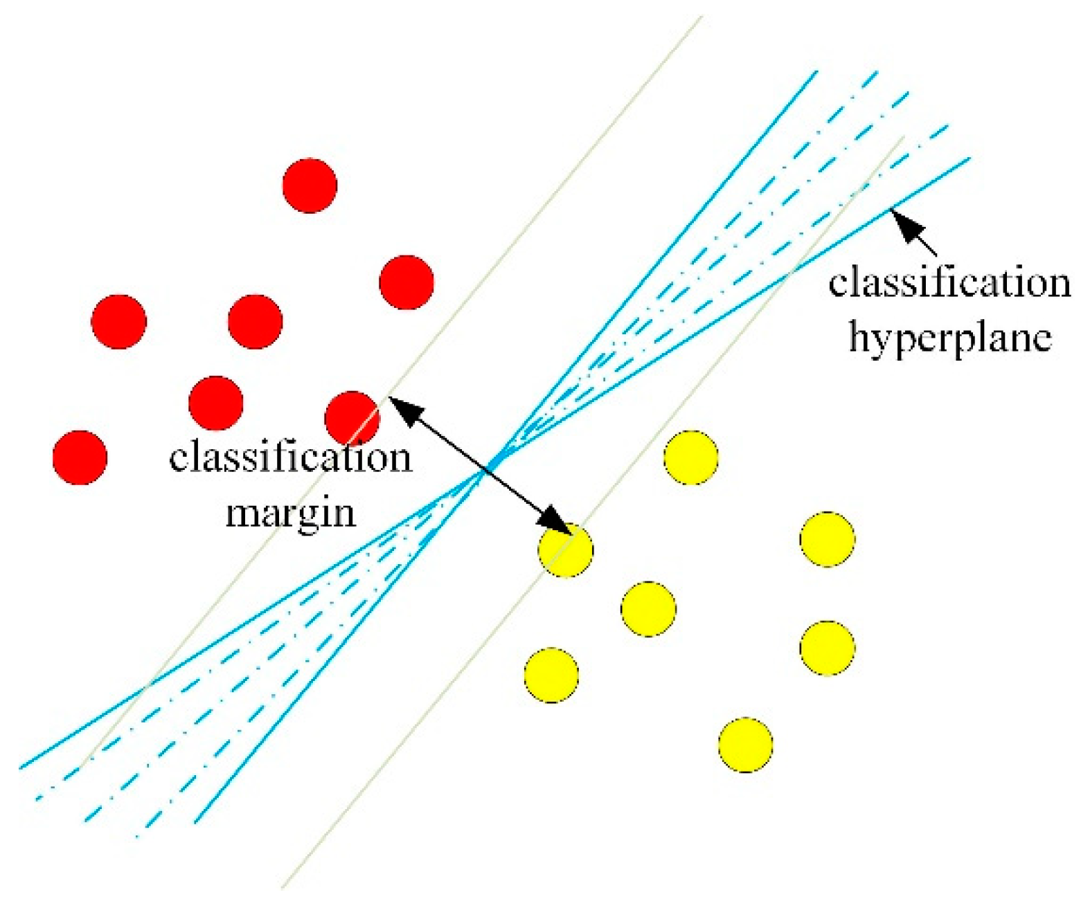
where R denotes the number of rank-1 projecting tensors. In Equation (14), the hyperplane is defined by the sum of R rank-1 projection tensors (i.e., the rank-R projecting tensor ). The illustration of hyperplanes defined by rank-1 projecting tensor and hyperplanes defined by rank-R tensor is shown in Figure 3. It is seen that the linear combination of rank-1 projecting tensors can be used to obtain the hyperplane with more orientations, which indicates that the rank-R projection tensor is likely to obtain a more effective hyperplane.
Note that the multiclass classification mechanism of Equation (14) is equivalent to that of multiclass SVM (see Equation (9)). In other words, the multiclass classification mechanism of Equation (14) can be described as an OVR strategy that solves M hyperplanes simultaneously, of which mth hyperplane defined by is used to separate class m from the other. Considering the related research that the OVO strategy based SVM always achieves better results than OVR strategy based SVM, it is taken into consideration to embed OVO strategy to tensor space, of which the hyperplane defined by projection tensor is used to separate samples from class m and samples from class . In this way, the optimization problem in Equation (14) can be changed to the optimization problem in Equation (15).
where and denote the normal orientation of the hyperplane used to separate class m from class and the corresponding bias. Since OVR and OVO strategies have their own advantages, these two classification mechanisms are used as different versions of MCMS-STM to cope with different classification tasks.
3.1.2. Classify the Multiscale Objects without Image Resizing Preprocessing
For the objects to be classified presenting different sizes, the convention manner is to adjust slices of different sizes into the fixed size, whereas this operation is easy to lead to the loss of scale information or increase of background interferences.
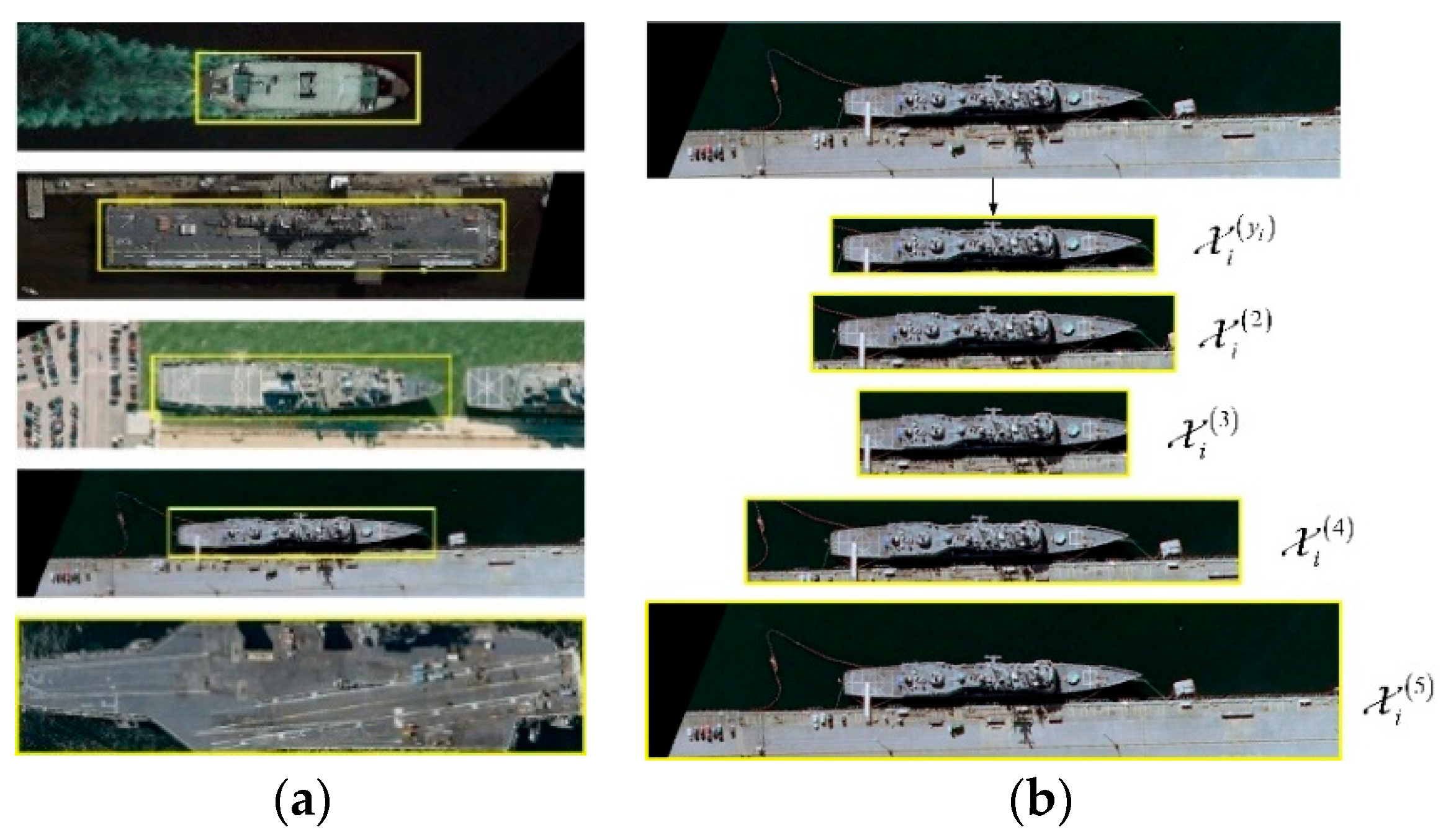
To maintain the scale information of objects and reduce the impact of background interferences, it is needed to extract slices with proper size to cover the object with a specific class, as shown in Figure 4. Assuming that each class of object presents a specific size, it is necessary to extract M sizes of slices of different sizes. Even for the same object, M slices of different sizes still need to be extracted because the category of the test sample is unknown (see Figure 4b). Therefore, different from the conventional manner that each object is described as a fixed-size slice, for each object, it is needed to extract M sizes of slices represented M-scale tensors . In this way, a multiscale sample set is constructed, where denotes the slice of mth size containing ith object. To separate input represented as M-scale tensors in tensor space, it is also required to construct projection tensors with M scales, i.e., , where the projection tensor with specific dimension is used to separate input slice with specific scale. In this way, the classification model in Equation (15) can be further extended to identify the multiscale objects without image resizing operation, and the corresponding optimization problem is shown in Equation (16).
Equation (16) is the final optimization problem of OVO version of MCMS-STM. For OVR version of MCMS-STM, the final optimization problem is given directly as follows.
Note that the OVR version of MCMS-STM only uses M hyperplanes defined by to separate samples.
On the one hand, the proposed MCMS-STM can use multiscale tensors to capture the category and scale information of objects and utilize grouped rank-R tensors to improve the effectiveness of multiclass classification problems. On the other hand, it can be found that the optimization problem of MCMS-STM is more complex than the binary STM, which needs to establish a specific solving method to obtain the optimal parameters.
3.2. Solving of the Optimization Problem for MCMS-STM
Since the procedures of training OVO and OVR versions of MCMS-STM are similar, we only give the solving methods for the OVO version of the MCMS-STM in this section and put the solving methods for the OVR version of the MCMS-STM in the Appendix A.
To solve the optimization problem in Equation (16) effectively, an alternating optimization scheme [25] is adopted for model training, i.e., optimize by fixing the other normal vectors in the kth iteration, where . First, all the projection vectors are initialized using uniformly distributed random numbers within 0 to 1. Then, we can get the Lagrangian function for alternating optimization in the kth iteration as follows.
where and denote the dual variables, and and denote the dummy dual variables. Let the partial derivatives of with respect to the original variables be zeros. We have
Substituting Equation (19) and Equation (20) into Equation (18) yields the following Lagrangian dual problem.
where
For convenience, rewrite the dual problem in the matrix form as follows.
where , and
where
It is found from Equation (23) that the dual problem of MCMS-STM in kth iteration is the quadratic optimization in terms of , which can be solved by classical quadratic programing method (e.g., interior-point method [35]). According to the resulting , the can be updated using Equation (19).
Note that the values of the objective function (see Equation (16)) in each iteration form a bounded and nonincreasing sequence. Therefore, there is a finite limit for that sequence. To stop iterating at the proper time, the termination criteria are constructed in Equation (28).
Combined with Equation (29), the equations and inequalities in terms of b can be drawn in following:
where .
When the optimal solution is reached, the above equations and inequalities hold. Therefore, b can be calculated by following linear programming.
where , and denote the slacking variables used to maintain the feasibility of linear programming. Using the classical simplex method [37], the Equation (31) can be solved to obtain the optimal b. At present, the training procedure of MCMS-STM has been finished.
After training MCMS-STM, for any test sample , the following decision function is used to predict the corresponding label.
where operator denotes the number of elements in the set. Note that there may be multiple candidate classes that maximize the Equation (32). For this situation, just like the operation in [20], we simply select the candidate class with the smallest label as the predicted class.
3.3. Acceleration of Training of OVO Version of MCMS-STM
In this section, combining the existing decomposition algorithm [38], a MCMS-STM-oriented decomposition algorithm is presented to break the complex quadratic programming (QP) for dual problem of MCMS-STM (see Equation (23)) into a series of simple analytic QP problems to train the OVO version of MCMS-STM efficiently.
To solve the QP in Equation (23) efficiently, based on the idea of a general decomposition algorithm, the dual variables are split into working set and non-working set, where variables in the working set are updated, and those in the non-working set are fixed in each iteration. To select the proper variables as the working set, a graph-based constraints model is illustrated in Figure 5 to demonstrate the constraints in Equation (23) clearly.
As shown in Figure 5, there are vertices in the graph, where each vertex indicates a set of dual variables, i.e., . The constraints in Equation (23) can be described visually via the graph-based constraints model, where the value of dual variables in each vertex should be between 0 and C, and the sum of the values for dual variables contained in the vertices (i,j) is equal to that in vertex (i,j), i.e., the vertex with the same color in Figure 5 should have the same sum. Since updating the variables contained in the vertices of the same color does not affect the feasibility of other variables, it is taken into consideration to select variables from the vertices of the same color as the working set.
First, the zeros values are assigned to all the dual variables as the initial feasible solution of the dual problem in Equation (23). Subsequently, select a working set from the vertices with the same color and . For variables in and , the constraints can be described as follows.
After the terminal criteria are satisfied, the current is optimal. The decomposition algorithm for solving the dual problem of the OVO version of the MCMS-STM is summarized in Algorithm 1.
| Algorithm 1. Decomposition algorithm of solving the dual problem of OVO version of the MCMS-STM. |
| Input: the Q of the dual problem of MCMS-STM and the labels . |
| Output: optimal a |
| for vertex in |
| Step 1: Select working set using Equation (34). |
| If , continue; otherwise, perform Step 2. |
| Step 2: Calculate the step size using Equations (36) and (37), and update the variables in working set. |
| Step 3: If the terminal criteria are met, output the as optimal solution, and return. |
| end |
4. Discussion of the Multiclass Classification Mechanism Used in MCMS-STM
To analyze the multiclass classification mechanism used in MCMS-STM compared with the existing OVO and OVR strategy, a detailed discussion is carried out as follows.
4.1. Discussion of OVR Version of MCMS-STM Compared with OVR Strategy Based STM
Considering the hard margin (i.e., the ) based [25] with OVR strategy, it is required to construct M classifiers, where the mth classifier is used to separate the class m from the other M-1 classes, as shown in the following optimization problem.
where denotes the normal orientation for the mth hyperplane.
Then, let and for OVR version of MCMS-STM (see Equation (17)), the corresponding optimization problem can be converted to Equation (39).
By adding the two inequalities in Equation (38), it is easy to find that the feasible solution of Equation (38) is also the feasible solution of Equation (39). Thus, the solution of Equation (38) is the feasible solution of Equation (39), but not necessarily the optimal one. That means the MCMS-STM may obtain the optimal solution with a larger classification margin compared with using OVR strategy, i.e., the better generalization ability.
4.2. Discussion of OVO Version of MCMS-STM Compared with OVO Strategy Based STM
When using OVO strategy [20] based to process M class classification problems, classifiers are constructed, where each one is used to separate specific two classes. For separating classes m and m′, the corresponding optimization problem of is shown below.
where denote the normal orientation of the hyperplane and bias of the hyperplane, respectively. For OVO version of MCMS-STM (see Equation (16)), let the and . The corresponding optimization problem is shown below.
For any feasible solution of and in Equation (40), let and , we can obtain , , and as the feasible solution of Equation (41). On the contrary, for the constraints in Equation (41), we obtain:
According to Equation (42), the constraints in Equation (41) can be converted to the same form as the constraints in Equation (40). Note that the feasible solutions of different methods can be transformed into each other using simple operations. Therefore, the MCMS-STM has the OVO interpretation.
Through the above analysis, the MCMS-STM present both the OVR and OVO interpretations under the specific parameter setting. More importantly, compared with the OVR and OVO strategies that need to learn multiple classification hyperplanes separately, a remarkable advantage is that the MCMS-STM can learn the multiple classification hyperplanes simultaneously to mine the correlation between multiple classes.
5. Experiments and Analysis
To demonstrate the superiority of the MCMS-STM for multiclass multiscale object recognition, two datasets containing image slices of multiclass multiscale objects are used to evaluate the performance of the proposed MCMS-STM, and the detailed information of datasets is introduced as follows.
- (1)
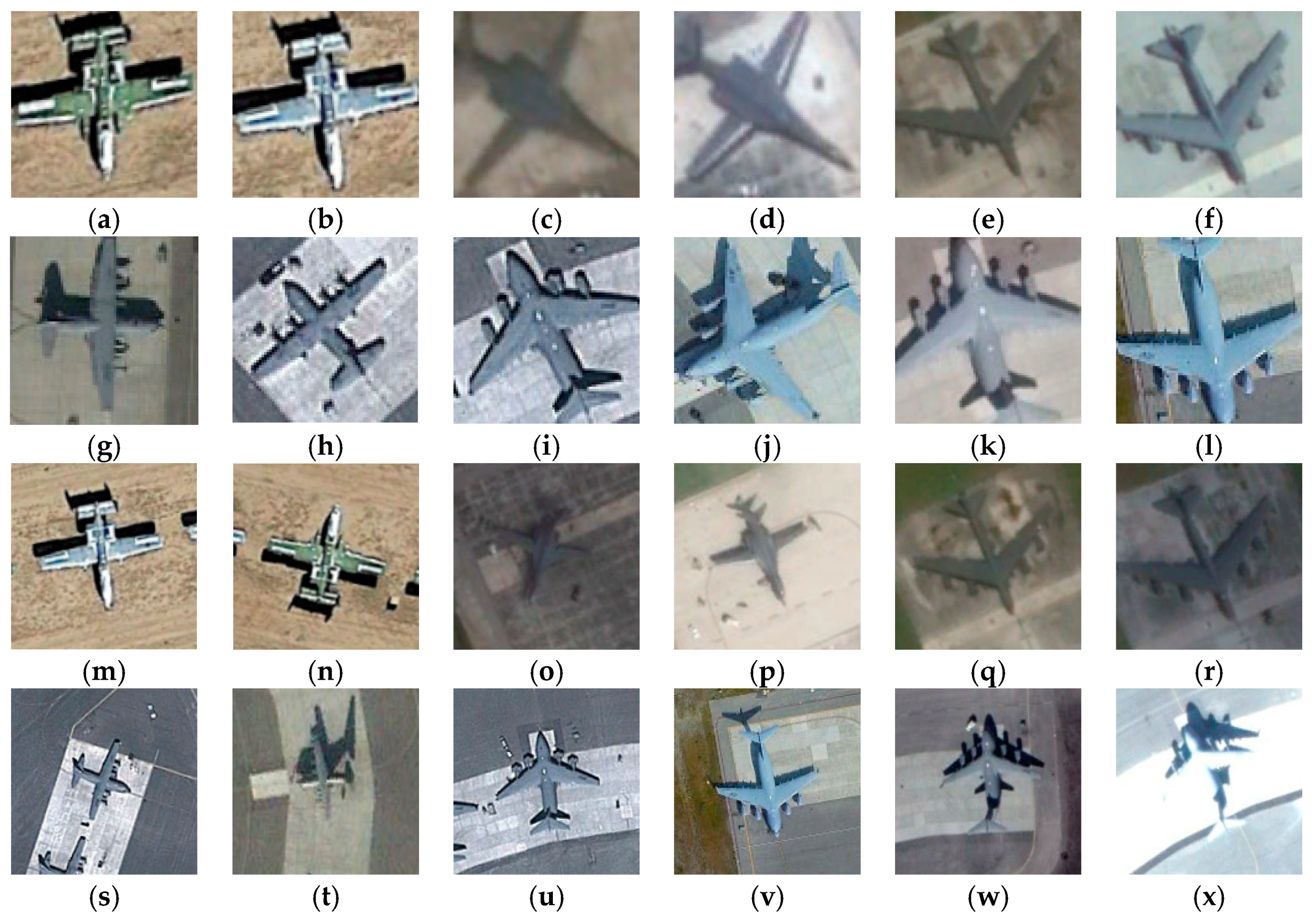
- Dataset 1: To verify the performance of MCMS-STM for multiclass multiscale airplane classification, the RSIs containing 218 airplanes with five types are collected from Google Earth service with a spatial resolution of 0.5 m and R, G, and B spectral bands. Then, using two image resizing operations, these 218 airplanes are cut separately from RSIs to build two slice sets. For slices set 1 generated from image resizing operation 1, the slices are cut according to the type of contained objects and then resized to a fixed size using a bilinear interpolation method. For slices set 2 generated from image resizing operation 2, these slices are cut at a size large enough (i.e., ) so that all the types of objects are contained completely in the corresponding slice. These slices contain various backgrounds, and the contained multiclass airplanes present different orientations and sizes. Some representative slices from two slices sets of dataset 1 are displayed in Figure 6.
- (2)
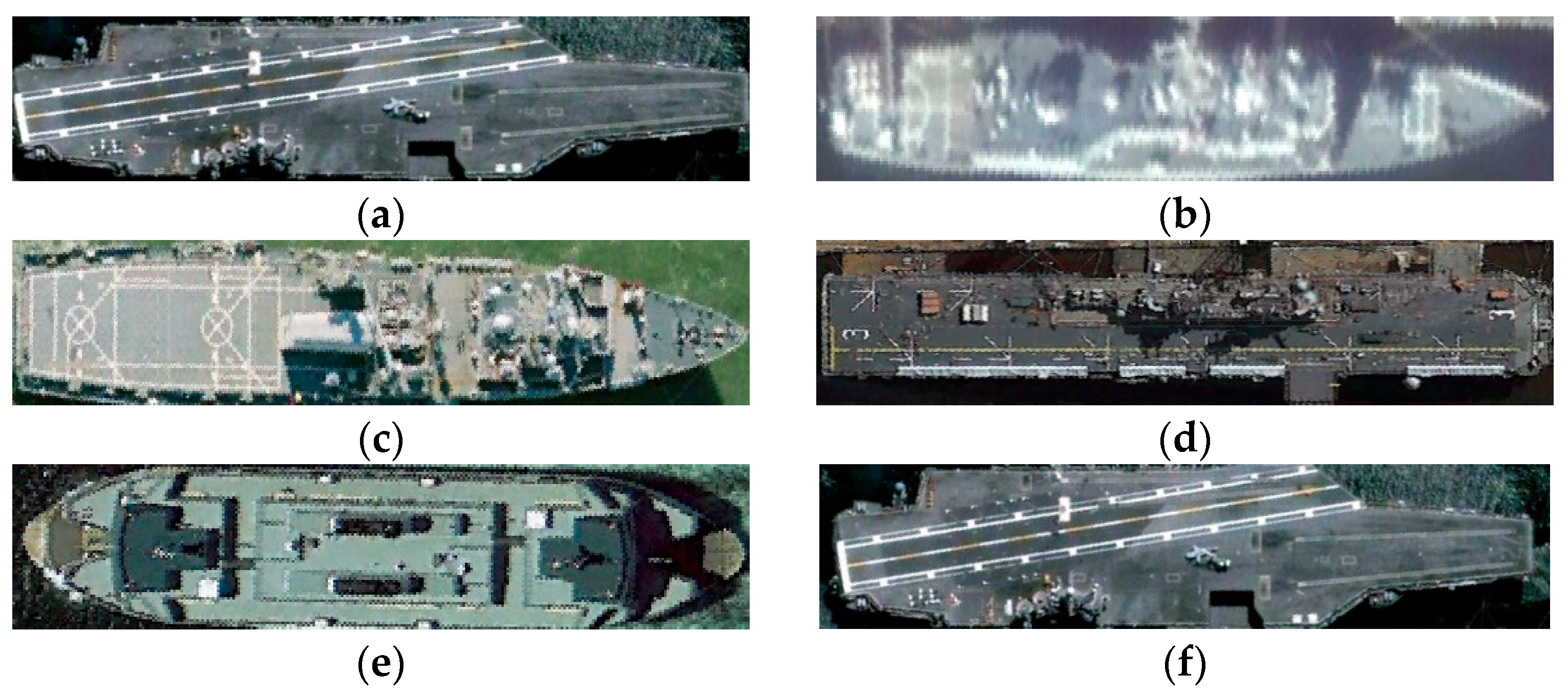
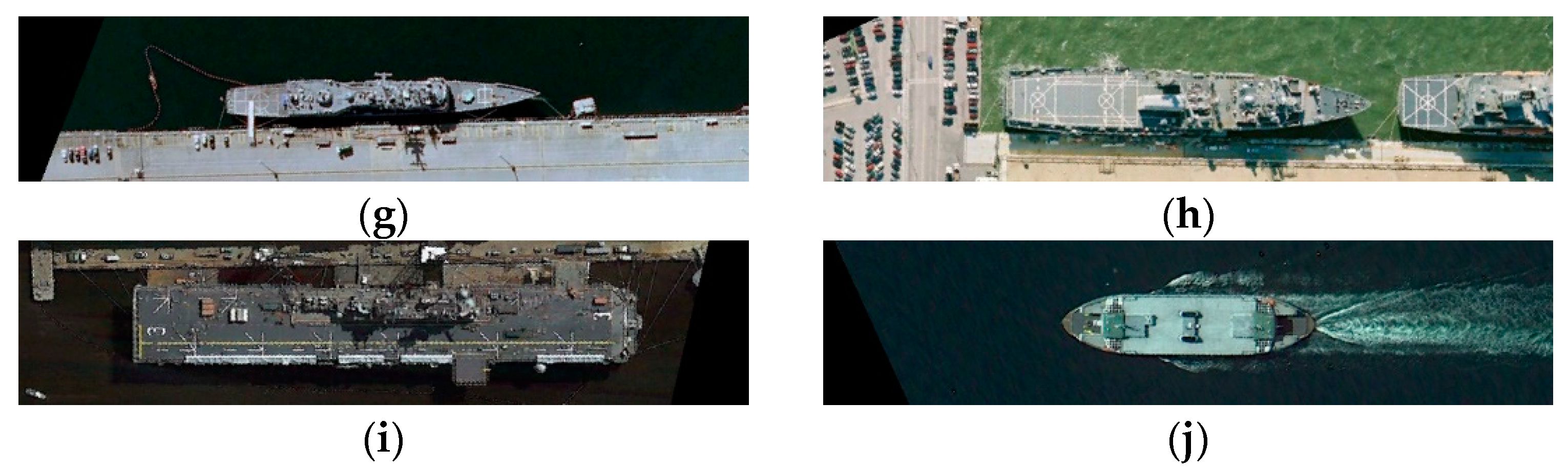
- Dataset 2: The HRSC-2016 [39] dataset contains 1070 harbor RSIs with R, G, and B spectral bands collected from Google Earth service. To evaluate the performance of MCMS-STM for multiscale object recognition, 342 ships with five types are sliced from HRSC-2016 whose spatial resolution is equal to 1.07 m. Similar to dataset 1, these slices are cut by two image resizing operations to form two slices set. For slices set 1 generated from image resizing operation 1, the slices are cut according to the type of contained objects and then resized to a fixed size using a bilinear interpolation method. For slices set 2 generated from image resizing operation 2, these slices are cut at a size large enough (i.e., ) to contain airplanes with different types. Some image slices with different types of ships in two slices sets of dataset 2 are shown in Figure 7.
The experiments are composed of four parts. In Section 5.1, the impact of parameter setting is analyzed. In Section 5.2, the affection of image resizing preprocessing for the recognition results is examined. In Section 5.3, the efficiency of the proposed decomposition algorithm is verified compared with the typical interior-point method and active-set method. In Section 5.4, the recognization accuracy of MCMS-STM is evaluated compared with typical SVM and STM methods using dataset 1 and dataset 2. In Section 5.5, the performance of MCMS-STM is further evaluated compared with typical deep learning methods. All the simulations are running on the computer with Windows 10 operating system and Intel i7-7700CPU at 3.6 G Hz.
The code of MCMS-STM can be found at https://github.com/supergt3/MCMS-STM (accessed on 23 November 2021).
5.1. Analysis of the Impact of Parameter Setting on Classification Performance
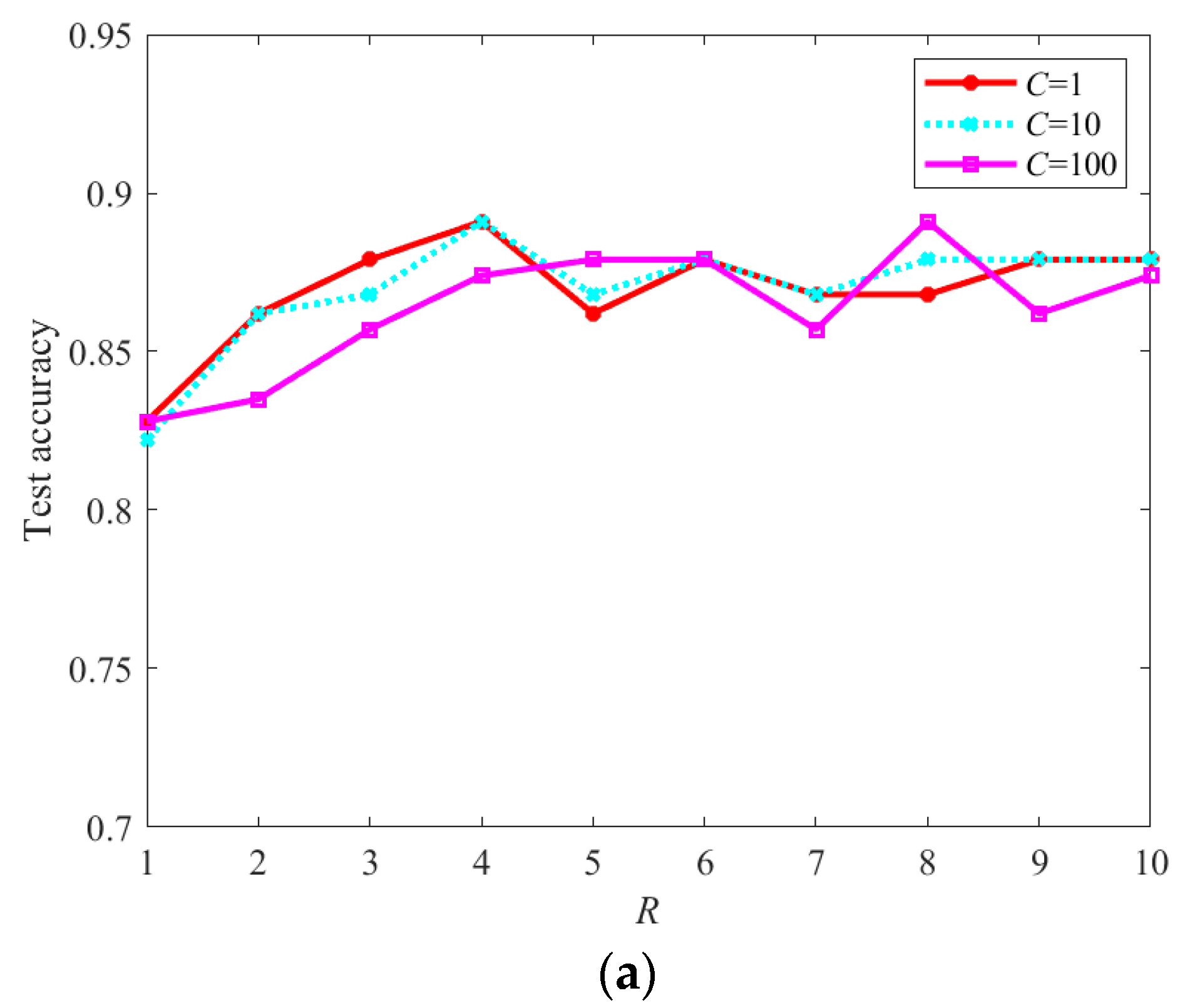
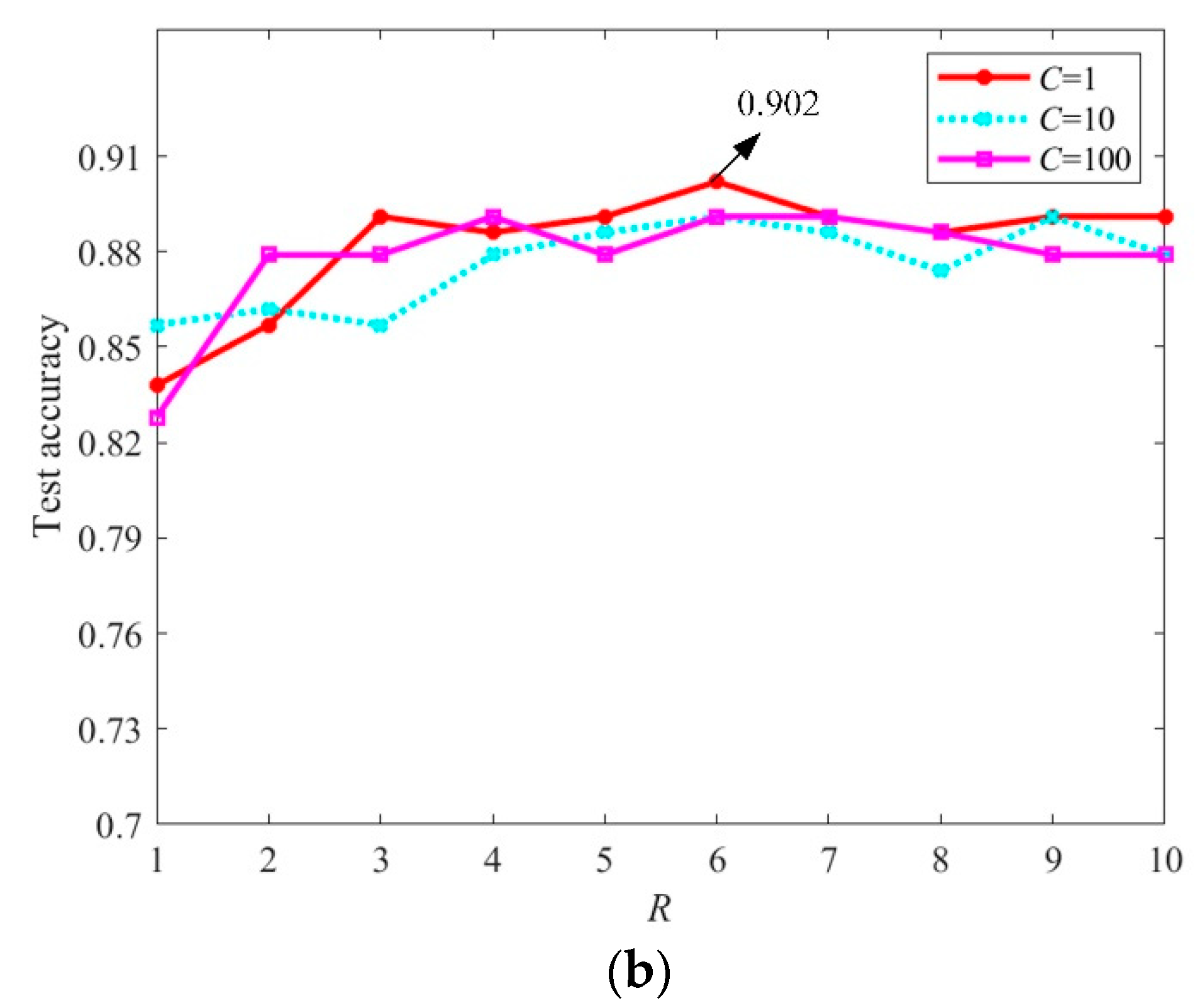
The main parameters in MCMS-STM include the R and C, which denote the CP rank of the projection tensor and the regularization parameter, respectively. To demonstrate the impact of parameter setting, the N-fold cross-validation method is adopted to partition the slices set 1 of dataset 1 into N subsets, and test the recognization accuracy using the one subset according to the trained classifier using the remaining N-1 subsets. This process is then repeated N times, with each of the N subsets used exactly once as the test samples. Through adjusting the values of R from and C from , the obtained classification accuracies of different versions of MCMS-STM are shown in Figure 8.
From Figure 8, it is observed that the recognization accuracy of MCMS-STM is affected by different parameter settings. In detail, it is seen that the increase of C may have a positive or negative effect on recognization accuracy for different values of R. Therefore, it is difficult to set an effective C in advance. In addition, for the case of using the same C, MCMS-STM with R < 3 obtains smaller recognization accuracy than that with , because the projection tensor with a small R is difficult to define an accurate classification hyperplane. Through observing Figure 8, it is found that the best recognization accuracy is obtained by OVO version of the MCMS-STM. The reason is probably that OVO version of the MCMS-STM may obtain a larger classification margin compared with OVR version of the MCMS-STM.
5.2. Analysis of the Impact of Image Resizing on Classification Performance
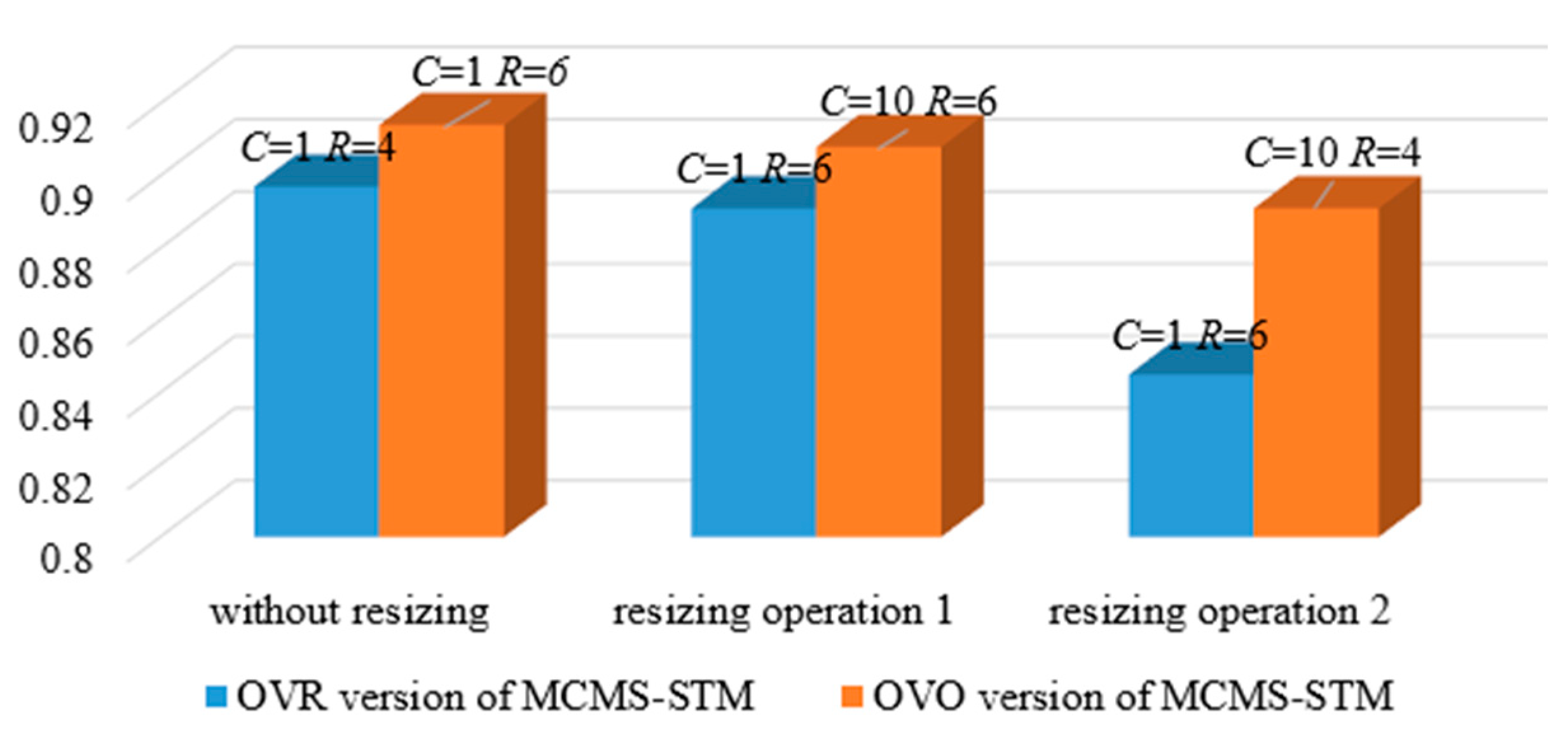
One of the significant advantages of the MCMS-STM method is that it can use multiscale projection tensors to effectively classify objects with different sizes, avoiding the loss of objects’ scale information caused by image resizing. To highlight the superiority of MCMS-STM, two slices sets obtained by different image resizing methods are utilized to examine the recognization accuracy of the MCMS-STM with multiscale projection tensors and single-scale projection tensors. The experiments are implemented in three control groups. In detail, for control group 1, the MCMS-STM with single-scale projection tensors and slices set 1 are utilized to obtain the classification results. For control group 2, the MCMS-STM with single-scale projection tensors and slices set 2 are utilized to obtain the classification results. For control group 3, the MCMS-STM with multiscale projection tensors and the slices set 1 are utilized to obtain the classification results. To use multiscale projection tensors, it is needed to decide the sizes of multiscale tensors. In the experiments, the sizes of slices for five types of ships are set to , , , and , respectively, according to the average sizes of objects for the different types. The obtained classification results for MCMS-STM under different conditions are plotted in Figure 9.
The accuracy in Figure 9 denotes the largest accuracy with parameters C and R selected from and under different versions of MCMS-STM. For MCMS-STM, the OVO version indicates the larger classification margin, but at the same time, it will also cause misclassification because the decision function (see Equation (32)) may generate multiple results. Therefore, for dataset 2, it is observed that the recognization accuracy of OVR version of MCMS-STM is higher than that of OVO version of MCMS-STM. In addition, note that the resizing operation used to generate slices set 1 will lead to the loss of object’s scale information, and the resizing operation used to generate slices set 2 will bring excessive background interferences, i.e., the two resizing operations have their own disadvantages. In comparison, the multiscale projection tensors used in MCMS-STM can maintain the scale information of objects while avoiding excessive background interferences. Therefore, it is observed that the recognization accuracy of MCMS-STM without resizing operations is better than using MCMS-STM with resizing operations. The above analysis concludes that the MCMS-STM with multiscale projection tensors is effective for multiscale object recognition tasks.
5.3. Evaluation of the Performance of the Decomposition Algorithm for Training MCMS-STM
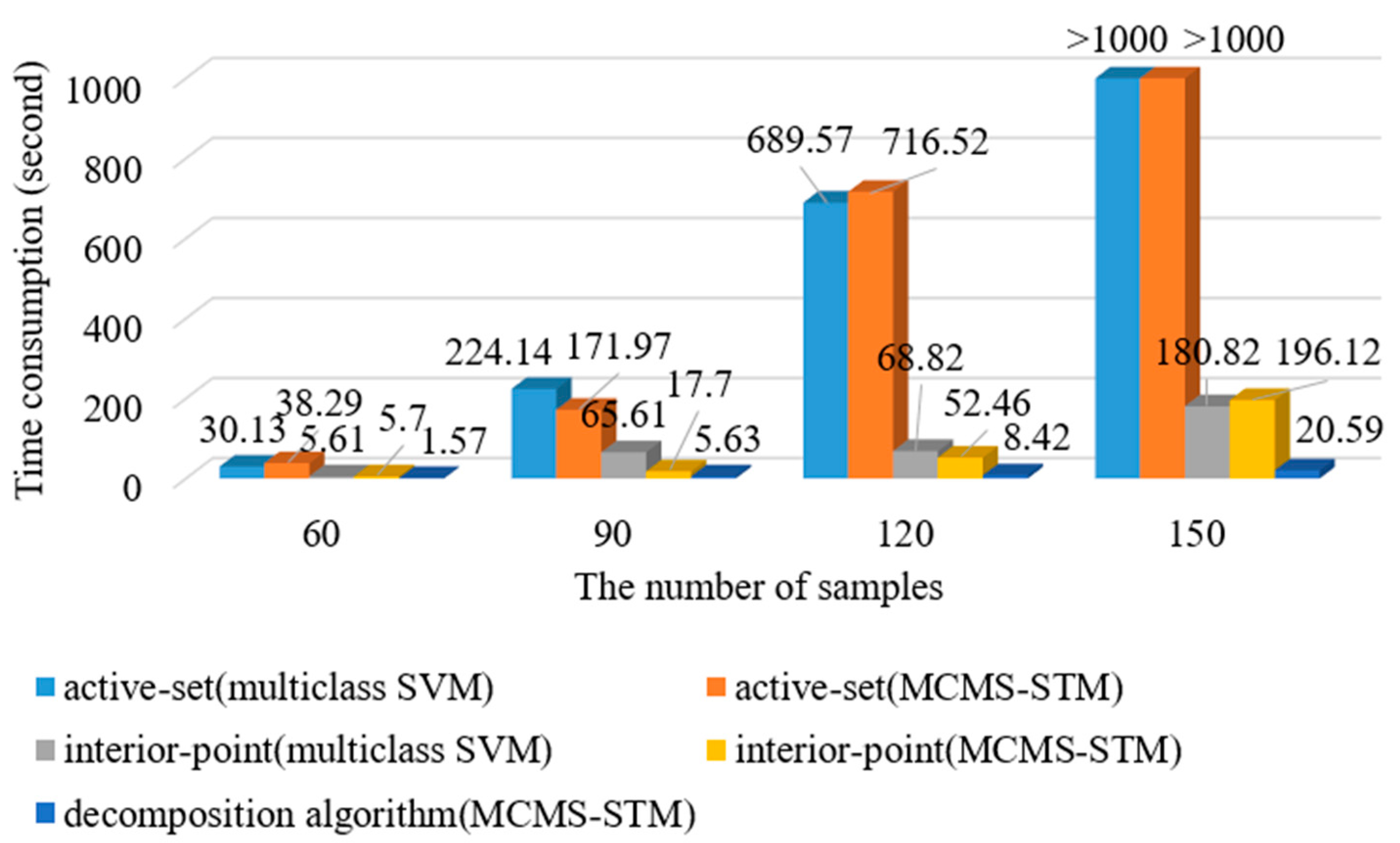
To verify the efficiency of the proposed decomposition algorithm for training OVO version of MCMS-STM, the experiments are conducted on dataset 1 to evaluate the time consumption of training MCMS-STM and classical multiclass SVM using different optimization solving algorithms, including the proposed decomposition algorithm, interior-point method [35] and active-set method [40], under different numbers of training samples, as shown in Figure 10.
The time consumption in Figure 10 represents the performing time to solve the dual problem of the MCMS-STM or multiclass SVM once. From Figure 10, when using the same optimization algorithm, i.e., interior-point algorithm or active-set algorithm, it can be seen that the time consumption of solving dual problem of MCMS-STM is similar to that of solving dual problem of multiclass SVM. In addition, it is seen that the time consumption of the interior-point algorithm is less than that of the active-set algorithm under different sizes of training sample sets. Remarkably, it can be seen that the proposed decomposition algorithm significantly reduces the time consumption compared with the interior-point method and active-set method for training MCMS-STM, especially for the training set with a larger size. It indicates the efficiency of the proposed decomposition algorithm for training the MCMS-STM, especially for the training set with a large size.
5.4. Evaluation of the Performance of MCMS-STM Compared with Existing SVM and STM Methods
In this section, the experiments are conducted on dataset 1 and dataset 2 to evaluate the performance of MCMS-STM for multiclass multiscale airplane classification and ship classification compared with typical SVM and STM methods. To avoid the classification results from being affected by different feature extraction algorithms, the image slices represented as tensors are used as input directly for all the classification methods. In detail, according to the size of different objects, the dimensions of multiscale tensors for airplanes with five types are set to for , , , and , respectively, and those for ships with five types are set to , , , and , respectively. The first order, second order and third order for multiscale tensors denote the horizontal spatial order, vertical spatial order, and spectral order, respectively. For the comparison methods, two slice sets from dataset 1 and dataset 2 obtained by different slice cropping methods are utilized to obtain the classification results under two types of image resizing operations, respectively. In addition, note that the SVM and STM methods can only deal with bi-category classification problems. Therefore, the OVO and OVR strategies are introduced to perform multiclass classifications for binary SVM and STM methods indirectly. Considering that the SVM method cannot process tensors directly, the vectorization operation is utilized to convert image slice to vector to comply with its input requirement. Then, all the methods select parameters from , and that corresponds to the best classification results to obtain the final recognization accuracy. Using the N-fold cross-validation, the accuracies of MCMS-STM for different classification tasks under different conditions are displayed in Table 3, Table 4, Table 5, and Table 6, respectively.
In these tables, the bolding accuracy indicates the best results, and the notation (OVO) 1 denotes using OVO strategy based under slice set 1. Overall, note that the classification results for 10-fold cross-validation are better than those for 5-fold cross-validation, mainly because the 10-fold cross-validation indicates that more samples are used for training. From these tables, it is observed that applying OVO strategy based comparison methods present better classification results than applying OVR strategy based comparison methods because the OVO is a competitive multiclass classification strategy compared with OVR strategy. For N-fold cross-validation, by comparing the classification accuracies between N = 5 and N = 10, it can be found that there is a minor difference between different N for STM methods and a significant difference between different N for SVM methods. The reason is that the SVM method is embedded with much more parameters, and thus it is easy to improve performance as the number of samples increases. In addition, it can be seen that the recognization accuracy of multiclass SVM is better than most comparison methods under OVR or OVO strategy. Since the two resizing operations have their own advantages and disadvantages, i.e., the first type of resizing operation can reduce the impact of background interferences, while it loses the scale information of object, and the image the second type of resizing operation can maintain the scale information of objects, while it brings much more interferences for objects with small size, it is observed that using the slices set 1 obtains the largest accuracy for ship recognization under 10-fold cross-validation (see Table 6), and using the slices set 2 obtains the largest accuracy for airplane recognization under 10-fold cross-validation (see Table 4). That means two image resizing operations present comparable results. Moreover, it is seen that the optimal R that corresponds to the largest accuracy is located at the range from 4 to 8, as the projection with small R is difficult to describe the effective classification hyperplane, and the projection tensor with large R is easy to over-fit the training samples. It is worth observing that the MCMS-STM gets the best classification results among all the methods for different classification tasks. In detail, MCMS-STM gets 89.5% and 91.4% recognization accuracy for airplane recognization and ship recognization, respectively, while the largest accuracies of comparison methods for airplane recognization and ship recognization are equal to 88.6% and 89.9%, respectively. Therefore, it is concluded that the MCMS-STM is more effective for multiclass multiscale object recognition using remote sensing images compared with the comparison methods.
In addition, to verify whether the MCMS-STM makes improvements from a statistical view, the statistical test is applied to analyze the performance of the MCMS-STM against the SVM and STM methods.
For convenience, the most commonly applied test method, i.e., right-tailed significance t-test [41], is used to test the null hypothesis H0 that the difference of accuracy between MCMS-STM and the competitor is equal to zero. On the other hand, the alternate hypothesis H1 is that the difference of accuracy between MCMS-STM and the competitor is greater than zero.
To obtain effective results, half of samples in dataset 1 are used to train a classifier, and the rest of the samples in dataset 1 are used to evaluate the recognization accuracy of trained classifier for five classes of airplanes. The same processing is performed for dataset 2. In this way, ten paired observations are obtained for the sign test. According to obtained ten paired observations, use paired-sample right-tailed significance t-test [41], and the resulting p-value for MCMS-STM against the other methods is shown in Table 7.
Where positive, negative, ties, and p-value denote the number of times that the MCMS-STM outperforms the comparison method, the number of times that the comparison method outperforms the MCMS-STM, the number of times that both the MCMS-STM and comparison method obtain the same results, and the probability of the observation under H0. From Table 7, it is found that all the p-values are less than 0.05. Therefore, the null hypothesis can be rejected at the 0.05 significance level for all the comparison methods. It indicates that the proposed MCMS-STM outperforms the existing SVM and STM methods from the view of statistics.
5.5. Evaluation of the Performance of MCMS-STM Compared with Deep Learning Methods
Compared with deep learning methods relying on a large number of training samples, the proposed MCMS-STM can recognize multiclass multiscale objects effectively using a small number of training samples. To verify this advantage, the experiments are conducted on datasets 1 and 2 to compare the recognition accuracies of the MCMS-STM with two deep learning methods, i.e., GhostNet [42] and ResNeXt networks [43], of which the GhostNet utilizes the Ghost module to improve the feature representation power of the conventional convolutional layer and the ResNeXt improved from deep residual networks can exploit the aggregated residual transformations to mine the effective features to improve the recognization results. When training the GhostNet and ResNeXt, the learning rate and the batch size are set to 0.001 and 128, respectively. Since these two deep learning methods can only deal with slices with a fixed size, the slice sets 1 from two datasets are used to examine their performances. For MCMS-STM, the multiscale projection tensors are exploited, and the detailed sizes of projection tensors can be found in Section 5.4. To compare the recognization results of the proposed OVO version of MCMS-STM with the deep learning methods under different sizes of training sets, different proportions of samples in the dataset are selected as training samples and the rest as test samples, and the obtained recognization results are shown in Table 8 and Table 9.
Where the notation p in Table 8 and Table 9 denotes the proportion of the training samples occupying the data set. From the above tables, it is observed that the recognization accuracy is generally improved with the increase of training set size because more training samples can ensure sufficient training of the classifier. In addition, it is seen that the GhostNet obtains better results than ResNeXt under the same p. It indicates that the GhostNet can extract more effective features using its Ghost module. Since the deep learning methods rely on a large number of training samples, they obtain worse results under a small p. Remarkably, it is worth noting that the proposed MCMS-STM obtains significantly better results compared to deep learning methods, especially when the training samples are small. This funding implies the superiority of the proposed MCMS-STM for the small sample case compared with the deep learning methods.
6. Conclusions
To classify the multiclass multiscale objects in RSIs effectively, the MCMS-STM is proposed incorporating multiple hyperplanes defined by multiscale projection tensors to map the input of object slices with different sizes to multiclass class space, getting rid of the conventional image resizing operation. The main contributions of this paper can be summarized in the three folds below.
- (1)
- To achieve multiclass classifications for objects in RSIs, the MCMS-STM is proposed to learn multiple hyperplanes defined by rank-R projection tensors simultaneously to map input represented as tensor into class space. This new multiclass classification mechanism makes it easy to construct the corresponding decomposition algorithm to accelerate the training of the MCMS-STM and enables the classifier to present OVO and OVR interpretations, ensuring the MCMS-STM can deal with different classifications tasks effectively.
- (2)
- To identify multiscale objects in RSIs, instead of the conventional image resizing operation, according to the object position obtained from detection results, multiple slices of different sizes are extracted to describe the contained object with unknown class, and multidimensional classification hyperplanes are established to separate input of multiple slices with different sizes to achieve cross-scale object recognition. This multiscale classification mechanism can avoid the loss of scale information and reduce the impact of background interferences caused by conventional image resizing preprocessing.
- (3)
- To accelerate the training of OVO version of MCMS-STM, combining graph-based analysis, a decomposition algorithm is proposed to break the dual problem of OVO version of MCMS-STM as a series of small sub-optimizations, reducing the time consumption caused by the large Q. It ensures the MCMS-STM can be trained efficiently for more samples and classes.
The future work will focus on extending the MCMS-STM to adapt to the objects with different orientations and constructing a universal decomposition algorithm to accelerate the training of different versions of MCMS-STM.
Author Contributions
Methodology, T.G.; project administration, H.C.; data curation, W.C. All authors have read and agreed to the published version of the manuscript.
Funding
This work was supported by the National Natural Science Foundation of China under Grant 61771170.
Institutional Review Board Statement
Not applicable.
Informed Consent Statement
Not applicable.
Data Availability Statement
Not applicable.
Conflicts of Interest
The authors declare no conflict of interest.
Appendix A
We give the procedure of training OVR version of MCMS-STM in this section. Similar to the solving method of OVO version of MCMS-STM, an alternating optimization scheme is adopted for training of OVR version of MCMS-STM, i.e., optimize by fixing the other normal vectors in the kth iteration, where . First, all the projection vectors are initialized using uniformly distributed random numbers within 0 to 1. Then, get the Lagrangian function for alternating optimization in kth iteration as follows.
Let the partial derivatives of with respect to the original variables be zeros. We have
Substituting Equations (A2) and (A3) into Equation (A1) yields the following Lagrangian dual problem.
where
Using quadratic programing method (e.g., interior-point method [35]), the optimization problem in Equation (A4) can be solved. Then, according to the resulting , the can be updated using Equation (A2). To stop iterating at the proper time, the termination criteria are constructed in Equation (A6).
where denotes the updated in the last iteration. To calculate bias b, we have
Then, the equations and inequalities in terms of b can be drawn in following:
where .
When the optimal solution is reached, the above equations and inequalities hold. Therefore, b can be calculated by following linear programming using the classical simplex method [37].
After training MCMS-STM, for any test sample , the following decision function is used to predict the corresponding label.
References
- Girshick, R. Fast r-cnn. In Proceedings of the IEEE International Conference on Computer Vision, Santiago, Chile, 13–16 December 2015; pp. 1440–1448. [Google Scholar]
- Ren, S.; He, K.; Girshick, R.; Sun, J. Faster r-cnn: Towards real-time object detection with region proposal networks. Adv. Neural Inf. Process. Syst. 2015, 28, 91–99. [Google Scholar] [CrossRef] [Green Version]
- Zhou, M.; Zou, Z.; Shi, Z.; Zeng, W.-J.; Gui, J. Local attention networks for occluded airplane detection in remote sensing images. IEEE Geosci. Remote Sens. Lett. 2019, 17, 381–385. [Google Scholar] [CrossRef]
- Pang, J.; Li, C.; Shi, J.; Xu, Z.; Feng, H. -CNN: Fast Tiny Object Detection in Large-scale Remote Sensing Images. IEEE Trans. Geosci. Remote Sens. 2019, 57, 5512–5524. [Google Scholar] [CrossRef] [Green Version]
- Liu, W.; Anguelov, D.; Erhan, D.; Szegedy, C.; Reed, S.; Fu, C.-Y.; Berg, A.C. Ssd: Single shot multibox detector. In Proceedings of the European Conference on Computer Vision, Amsterdam, The Netherlands, 8–16 October 2016; pp. 21–37. [Google Scholar]
- Redmon, J.; Divvala, S.; Girshick, R.; Farhadi, A. You only look once: Unified, real-time object detection. In Proceedings of the IEEE conference on computer vision and pattern recognition, Las Vegas, NV, USA, 27–30 June 2016; 2016; pp. 779–788. [Google Scholar]
- Dadsetan, S.; Pichler, D.; Wilson, D.; Hovakimyan, N.; Hobbs, J. Superpixels and Graph Convolutional Neural Networks for Efficient Detection of Nutrient Deficiency Stress from Aerial Imagery. In Proceedings of the IEEE/CVF Conference on Computer Vision and Pattern Recognition, Virtual, 19–25 June 2021; pp. 2950–2959. [Google Scholar]
- Hong, D.; He, W.; Yokoya, N.; Yao, J.; Gao, L.; Zhang, L.; Chanussot, J.; Zhu, X. Interpretable hyperspectral artificial intelligence: When nonconvex modeling meets hyperspectral remote sensing. IEEE Geosci. Remote Sens. Mag. 2021, 9, 52–87. [Google Scholar] [CrossRef]
- Hong, D.; Gao, L.; Yokoya, N.; Yao, J.; Chanussot, J.; Du, Q.; Zhang, B. More diverse means better: Multimodal deep learning meets remote-sensing imagery classification. IEEE Trans. Geosci. Remote Sens. 2020, 59, 4340–4354. [Google Scholar] [CrossRef]
- Long, Y.; Gong, Y.; Xiao, Z.; Liu, Q. Accurate object localization in remote sensing images based on convolutional neural networks. IEEE Trans. Geosci. Remote Sens. 2017, 55, 2486–2498. [Google Scholar] [CrossRef]
- Cheng, G.; Zhou, P.; Han, J. Learning rotation-invariant convolutional neural networks for object detection in VHR optical remote sensing images. IEEE Trans. Geosci. Remote Sens. 2016, 54, 7405–7415. [Google Scholar] [CrossRef]
- Nguyen, V.D.; Tran, D.T.; Byun, J.Y.; Jeon, J.W. Real-time vehicle detection using an effective region proposal-based depth and 3-channel pattern. IEEE Trans. Intell. Transp. Syst. 2018, 20, 3634–3646. [Google Scholar] [CrossRef]
- Chen, H.; Zhao, J.; Gao, T.; Chen, W. Fast airplane detection with hierarchical structure in large scene remote sensing images at high spatial resolution. In Proceedings of the IGARSS 2018-2018 IEEE International Geoscience and Remote Sensing Symposium, Valencia, Spain, 22–27 July 2018; pp. 4846–4849. [Google Scholar]
- An, Z.; Shi, Z.; Teng, X.; Yu, X.; Tang, W. An automated airplane detection system for large panchromatic image with high spatial resolution. Optik 2014, 125, 2768–2775. [Google Scholar] [CrossRef]
- Zhang, L.; Zhang, Y. Airport detection and aircraft recognition based on two-layer saliency model in high spatial resolution remote-sensing images. IEEE J. Sel. Top. Appl. Earth Obs. Remote Sens. 2016, 10, 1511–1524. [Google Scholar] [CrossRef]
- Jing, M.; Zhao, D.; Zhou, M.; Gao, Y.; Jiang, Z.; Shi, Z. Unsupervised oil tank detection by shape-guide saliency model. IEEE Geosci. Remote Sens. Lett. 2018, 16, 477–481. [Google Scholar] [CrossRef]
- Cortes, C.; Vapnik, V. Support-vector networks. Mach. Learn. 1995, 20, 273–297. [Google Scholar] [CrossRef]
- Schölkopf, B.; Smola, A.J.; Williamson, R.C.; Bartlett, P.L. New support vector algorithms. Neural Comput. 2000, 12, 1207–1245. [Google Scholar] [CrossRef]
- Suykens, J.A.; Vandewalle, J. Least squares support vector machine classifiers. Neural Process. Lett. 1999, 9, 293–300. [Google Scholar] [CrossRef]
- Chang, C.-C.; Lin, C.-J. LIBSVM: A library for support vector machines. ACM Trans. Intell. Syst. Technol. (TIST) 2011, 2, 1–27. [Google Scholar] [CrossRef]
- Godbole, S.; Sarawagi, S.; Chakrabarti, S. Scaling multi-class support vector machines using inter-class confusion. In Proceedings of the Eighth ACM SIGKDD International Conference on Knowledge Discovery and Data Mining, Edmonton, AB, Canada, 23–26 July 2002; pp. 513–518. [Google Scholar]
- Weston, J.; Watkins, C. Support vector machines for multi-class pattern recognition. In Proceedings of the ESANN 1999, 7th European Symposium on Artificial Neural Networks, Bruges, Belgium, 21–23 April 1999; pp. 219–224. [Google Scholar]
- Iosifidis, A.; Gabbouj, M. Multi-class support vector machine classifiers using intrinsic and penalty graphs. Pattern Recognit. 2016, 55, 231–246. [Google Scholar] [CrossRef]
- De Lima, M.D.; Costa, N.L.; Barbosa, R. Improvements on least squares twin multi-class classification support vector machine. Neurocomputing 2018, 313, 196–205. [Google Scholar] [CrossRef]
- Tao, D.; Li, X.; Wu, X.; Hu, W.; Maybank, S.J. Supervised tensor learning. Knowl. Inf. Syst. 2007, 1, 1–42. [Google Scholar] [CrossRef]
- Hao, Z.; He, L.; Chen, B.; Yang, X. A linear support higher-order tensor machine for classification. IEEE Trans. Image Process. 2013, 22, 2911–2920. [Google Scholar]
- Chen, Z.-Y.; Fan, Z.-P.; Sun, M. A multi-kernel support tensor machine for classification with multitype multiway data and an application to cross-selling recommendations. Eur. J. Oper. Res. 2016, 255, 110–120. [Google Scholar] [CrossRef]
- Kotsia, I.; Guo, W.; Patras, I. Higher rank support tensor machines for visual recognition. Pattern Recognit. 2012, 45, 4192–4203. [Google Scholar] [CrossRef]
- Kotsia, I.; Patras, I. Support tucker machines. In Proceedings of the CVPR 2011, Colorado Springs, CO, USA, 20–25 June 2011; pp. 633–640. [Google Scholar]
- Ma, Z.; Yang, L.T.; Zhang, Q. Support Multimode Tensor Machine for Multiple Classification on Industrial Big Data. IEEE Trans. Ind. Inform. 2020, 17, 3382–3390. [Google Scholar] [CrossRef]
- Hsu, C.-W.; Lin, C.-J. A comparison of methods for multiclass support vector machines. IEEE Trans. Neural Netw. 2002, 13, 415–425. [Google Scholar] [PubMed] [Green Version]
- Xie, J.; He, N.; Fang, L.; Plaza, A. Scale-free convolutional neural network for remote sensing scene classification. IEEE Trans. Geosci. Remote Sens. 2019, 57, 6916–6928. [Google Scholar] [CrossRef]
- Kolda, T.G.; Bader, B.W. Tensor decompositions and applications. SIAM Rev. 2009, 51, 455–500. [Google Scholar] [CrossRef]
- Savicky, P.; Vomlel, J. Exploiting tensor rank-one decomposition in probabilistic inference. Kybernetika 2007, 43, 747–764. [Google Scholar]
- Momoh, J.A.; Guo, S.; Ogbuobiri, E.; Adapa, R. The quadratic interior point method solving power system optimization problems. IEEE Trans. Power Syst. 1994, 9, 1327–1336. [Google Scholar] [CrossRef]
- Boyd, S.; Boyd, S.P.; Vandenberghe, L. Convex Optimization; Cambridge University Press: Cambridge, UK, 2004. [Google Scholar]
- Brearley, A.L.; Mitra, G.; Williams, H.P. Analysis of mathematical programming problems prior to applying the simplex algorithm. Math. Program. 1975, 8, 54–83. [Google Scholar]
- Chang, C.-C.; Lin, C.-J. Trainings nu-support vector classifiers: Theory and algorithms. Neural Comput. 2001, 13, 2119–2147. [Google Scholar] [CrossRef]
- Liu, Z.; Wang, H.; Weng, L.; Yang, Y. Ship rotated bounding box space for ship extraction from high-resolution optical satellite images with complex backgrounds. IEEE Geosci. Remote Sens. Lett. 2016, 13, 1074–1078. [Google Scholar] [CrossRef]
- Bartlett, R.A.; Biegler, L.T. QPSchur: A dual, active-set, Schur-complement method for large-scale and structured convex quadratic programming. Optim. Eng. 2006, 7, 5–32. [Google Scholar] [CrossRef] [Green Version]
- Rohatgi, V.K.; Saleh, A.M.E. An Introduction to Probability and Statistics; John Wiley & Sons: Hoboken, NJ, USA, 2015. [Google Scholar]
- Han, K.; Wang, Y.; Tian, Q.; Guo, J.; Xu, C. GhostNet: More Features from Cheap Operations. In Proceedings of the 2020 IEEE/CVF Conference on Computer Vision and Pattern Recognition, Virtual, 14–29 June 2020. [Google Scholar]
- Xie, S.; Girshick, R.; Dollár, P.; Tu, Z.; He, K. Aggregated residual transformations for deep neural networks. In Proceedings of the IEEE Conference on Computer Vision and Pattern Recognition, Honolulu, HI, USA, 21–26 July 2017; pp. 1492–1500. [Google Scholar]
Figure 1.
Examples of two types of image normalization methods.

Figure 2.
Illustration of objects classification for MCMS-STM.

Figure 3.
Illustration of classification hyperplane defined by rank-1 projection tensor and rank-R projection tensor. The bule solid line denotes the hyperplane defined by rank-1 or rank-R tensor, and the blue dotted line denotes the hyperplane defined by rank-R tensor.
Figure 3.
Illustration of classification hyperplane defined by rank-1 projection tensor and rank-R projection tensor. The bule solid line denotes the hyperplane defined by rank-1 or rank-R tensor, and the blue dotted line denotes the hyperplane defined by rank-R tensor.

Figure 4.
Illustration of slices with proper sizes and multiscale slices. (a) Proper sizes of slices for different objects (b) illustration of multiscale slice.
Figure 4.
Illustration of slices with proper sizes and multiscale slices. (a) Proper sizes of slices for different objects (b) illustration of multiscale slice.

Figure 5.
Graph based constraints model. Each vertex in the graph indicates a set of dual variables, and the sum of each vertex with the same color is equal.
Figure 5.
Graph based constraints model. Each vertex in the graph indicates a set of dual variables, and the sum of each vertex with the same color is equal.

Figure 6.
Airplanes slices with different types from two slices sets of dataset 1. (a–l) are from slices set 1 of dataset 1, and (m–x) are from slices set 2 of dataset 1.
Figure 6.
Airplanes slices with different types from two slices sets of dataset 1. (a–l) are from slices set 1 of dataset 1, and (m–x) are from slices set 2 of dataset 1.

Figure 7.
Ship slices from two slices sets of dataset 2. (a–e) are from slices set 1 of dataset 2, and (f–j) are from slices set 2 of dataset 2.
Figure 7.
Ship slices from two slices sets of dataset 2. (a–e) are from slices set 1 of dataset 2, and (f–j) are from slices set 2 of dataset 2.


Figure 8.
The classification accuracies of MCMS-STM under different R and C using dataset 1. (a) The classification accuracies of OVR version of MCMS-STM with different R and C; (b) The classification accuracies of OVO version of MCMS-STM with different R and C.
Figure 8.
The classification accuracies of MCMS-STM under different R and C using dataset 1. (a) The classification accuracies of OVR version of MCMS-STM with different R and C; (b) The classification accuracies of OVO version of MCMS-STM with different R and C.


Figure 9.
The classification accuracies of MCMS-STM with or without different image resizing operations.
Figure 9.
The classification accuracies of MCMS-STM with or without different image resizing operations.

Figure 10.
The time consumption of solving the dual problem of MCMS-STM and multiclass SVM using different optimization solving algorithms under different numbers of training samples.
Figure 10.
The time consumption of solving the dual problem of MCMS-STM and multiclass SVM using different optimization solving algorithms under different numbers of training samples.


Table 1.
The symbols and their corresponding description used in this paper.
| Symbol | Description |
|---|---|
| lowercase letters (e.g., x,y) | scalar |
| lowercase boldface letters (e.g., x,y) | vector |
| uppercase boldface letter (e.g., M) | matrix |
| calligraphy letter (e.g., ) | tensor |
Table 2.
The description of notations and abbreviations for the proposed MCMS-STM.
| Notations and Abbreviations | Description |
|---|---|
| M | the number of classes, as well as the number of scales. |
| R | the CP rank of projection tensor. |
| L | the number of orders for projection tensor. |
| the projection vector of mode-l used to separate class m from others | |
| slacking variable | |
| C | regularization parameter |
| the bias used to separate class yi from class m | |
| the bias used to separate class yi from others | |
| dual variable | |
| SVM | support vector machine |
| STM | support tensor machine |
| OVO | one-versus-one |
| OVR | one-versus-rest |
| CP | CANDECOMP/PARAFAC |
Table 3.
The accuracies of different methods for multiscale airplanes recognization using 5-fold cross-validation.
Table 3.
The accuracies of different methods for multiscale airplanes recognization using 5-fold cross-validation.
| Method | Parameter Setting | Accuracy |
|---|---|---|
| OVR version of MCMS-STM | C = 1 R = 8 | 84.9% |
| OVO version of MCMS-STM | C = 1 R = 6 | 85.3% |
| (OVO) 1 | C = 10 | 82.2% |
| (OVR) 1 | C = 100 | 73.8% |
| (OVO) 1 | 80.7% | |
| (OVR) 1 | 76.2% | |
| Multi-class SVM1 | C = 100 | 82.6% |
| (OVO) 1 | C = 10 | 71.4% |
| (OVR) 1 | C = 1 | 66.5% |
| (OVO)2 | C = 10 | 79.4% |
| (OVR) 2 | C = 100 | 77.1% |
| (OVO) 2 | 80.3% | |
| (OVR) 2 | 75.2% | |
| Multi-class SVM2 | C = 10 | 81.7% |
| (OVO) 2 | C = 1 | 75.2% |
| (OVR) 2 | C = 1 | 70.6% |
Table 4.
The accuracies of different methods for multiscale airplanes recognization using 10-fold cross-validation.
Table 4.
The accuracies of different methods for multiscale airplanes recognization using 10-fold cross-validation.
| Parameter Setting | Accuracy | |
| OVR version of MCMS-STM | C = 10 R = 8 | 88.1% |
| OVO version of MCMS-STM | C = 10 R = 8 | 89.5% |
| (OVO) 1 | C = 10 | 84.0% |
| (OVR) 1 | C = 1 | 76.6% |
| (OVO) 1 | 85.3% | |
| (OVR) 1 | 77.3% | |
| Multi-class SVM1 | C = 1 | 85.3% |
| (OVO) 1 | C = 100 | 79.4% |
| (OVR) 1 | C = 1 | 74.8% |
| (OVO)2 | C = 100 | 87.6% |
| (OVR) 2 | C = 1 | 78.0% |
| (OVO) 2 | 88.6% | |
| (OVR) 2 | 79.4% | |
| Multi-class SVM2 | C = 100 | 88.1% |
| (OVO) 2 | C = 1 | 77.5% |
| (OVR) 2 | C = 1 | 71.2% |
Table 5.
The accuracies of different methods for multiscale ships recognization using 5-fold cross-validation.
Table 5.
The accuracies of different methods for multiscale ships recognization using 5-fold cross-validation.
| Method | Parameter Setting | Accuracy |
| OVR version of MCMS-STM | C = 100 R = 6 | 90.2% |
| OVO version of MCMS-STM | C = 1 R = 6 | 87.4% |
| (OVO) 1 | C = 1 | 86.1% |
| (OVR) 1 | C = 1 | 80.7% |
| (OVO) 1 | 86.1% | |
| (OVR) 1 | 79.0% | |
| Multi-class SVM1 | C = 1 | 85.3% |
| (OVO) 1 | C = 10 | 76.9% |
| (OVR) 1 | C = 1 | 73.1% |
| (OVO)2 | C = 10 | 83.3% |
| (OVR) 2 | C = 100 | 79.2% |
| (OVO) 2 | 84.5% | |
| (OVR) 2 | 79.5% | |
| Multi-class SVM2 | C = 100 | 84.2% |
| (OVO) 2 | C = 1 | 77.0% |
| (OVR) 2 | C = 1 | 70.6% |
Table 6.
The accuracies of different methods for multiscale ships recognization using 10-fold cross-validation.
Table 6.
The accuracies of different methods for multiscale ships recognization using 10-fold cross-validation.
| Method | Parameter Setting | Accuracy |
| OVR version of MCMS-STM | C = 10 R = 8 | 87.7% |
| OVO version of MCMS-STM | C = 1 R = 8 | 91.4% |
| (OVO) 1 | C = 1 | 87.4% |
| (OVR) 1 | C = 100 | 83.6% |
| (OVO) 1 | 87.0% | |
| (OVR) 1 | 82.4% | |
| Multi-class SVM1 | C = 1 | 89.9% |
| (OVO) 1 | C = 1 | 78.2% |
| (OVR) 1 | C = 1 | 74.4% |
| (OVO)2 | C = 100 | 85.6% |
| (OVR) 2 | C = 1 | 81.0% |
| (OVO) 2 | 86.2% | |
| (OVR) 2 | 80.5% | |
| Multi-class SVM2 | C = 100 | 86.2% |
| (OVO) 2 | C = 1 | 76.4% |
| (OVR) 2 | C = 10 | 69.6% |
Table 7.
The accuracies of different methods using the second type of normalization operation for multiscale airplanes classification using 10-fold cross-validation.
Table 7.
The accuracies of different methods using the second type of normalization operation for multiscale airplanes classification using 10-fold cross-validation.
| Method | Positive | Negative | Ties | p-Value |
|---|---|---|---|---|
| (OVO) | 9 | 0 | 1 | <0.0001 |
| (OVR) | 8 | 1 | 1 | 0.0045 |
| (OVO) | 9 | 0 | 1 | <0.0001 |
| (OVR) | 8 | 2 | 0 | 0.0049 |
| Multi-class SVM | 8 | 0 | 2 | 0.0097 |
| (OVO) | 9 | 0 | 1 | <0.0001 |
| (OVR) | 10 | 0 | 0 | <0.0001 |
Table 8.
The accuracies of the MCMS-STM and deep learning methods for dataset 1 under different numbers of training samples.
Table 8.
The accuracies of the MCMS-STM and deep learning methods for dataset 1 under different numbers of training samples.
| p = 0.1 | p = 0.2 | p = 0.3 | p = 0.4 | p = 0.5 | |
|---|---|---|---|---|---|
| GhostNet | 47.09% | 48.50% | 57.82% | 61.42% | 71.03% |
| ResNeXt | 40.86% | 46.06% | 52.08% | 54.84% | 60.19% |
| MCMS-STM | 61.73% | 63.79% | 73.20% | 79.39% | 81.65% |
Table 9.
The accuracies of the MCMS-STM and deep learning methods for dataset 2 under different numbers of training samples.
Table 9.
The accuracies of the MCMS-STM and deep learning methods for dataset 2 under different numbers of training samples.
| p = 0.1 | p = 0.2 | p = 0.3 | p = 0.4 | p = 0.5 | |
|---|---|---|---|---|---|
| GhostNet | 35.41% | 35.03% | 46.43% | 50.66% | 56.31% |
| ResNeXt | 30.37% | 34.97% | 44.64% | 47.74% | 54.23% |
| MCMS-STM | 62.21% | 70.07% | 70.29% | 74.76% | 79.53% |
Publisher’s Note: MDPI stays neutral with regard to jurisdictional claims in published maps and institutional affiliations. |
© 2022 by the authors. Licensee MDPI, Basel, Switzerland. This article is an open access article distributed under the terms and conditions of the Creative Commons Attribution (CC BY) license (https://creativecommons.org/licenses/by/4.0/).
Share and Cite
MDPI and ACS Style
Gao, T.; Chen, H.; Chen, W. MCMS-STM: An Extension of Support Tensor Machine for Multiclass Multiscale Object Recognition in Remote Sensing Images. Remote Sens. 2022, 14, 196. https://doi.org/10.3390/rs14010196
AMA Style
Gao T, Chen H, Chen W. MCMS-STM: An Extension of Support Tensor Machine for Multiclass Multiscale Object Recognition in Remote Sensing Images. Remote Sensing. 2022; 14(1):196. https://doi.org/10.3390/rs14010196
Chicago/Turabian StyleGao, Tong, Hao Chen, and Wen Chen. 2022. "MCMS-STM: An Extension of Support Tensor Machine for Multiclass Multiscale Object Recognition in Remote Sensing Images" Remote Sensing 14, no. 1: 196. https://doi.org/10.3390/rs14010196
Note that from the first issue of 2016, this journal uses article numbers instead of page numbers. See further details here.