
Assessment of CYGNSS Wind Speed Retrievals in Tropical Cyclones


Remote Sensing Systems, 444 10th Street, Suite 200, Santa Rosa, CA 95401, USA
*
Author to whom correspondence should be addressed.
Remote Sens. 2021, 13(24), 5110; https://doi.org/10.3390/rs13245110
Submission received: 17 November 2021
/
Revised: 9 December 2021
/
Accepted: 11 December 2021
/
Published: 16 December 2021
(This article belongs to the Special Issue Applications of GNSS Reflectometry for Earth Observation II)
Abstract
:The NASA CYGNSS satellite constellation measures ocean surface winds using the existing network of the Global Navigation Satellite System (GNSS) and was designed for measurements in tropical cyclones (TCs). Here, we focus on using a consistent methodology to validate multiple CYGNSS wind data records currently available to the public, some focusing on low to moderate wind speeds, others for high winds, a storm-centric product for TC analyses, and a wind dataset from NOAA that applies a track-wise bias correction. Our goal is to document their differences and provide guidance to users. The assessment of CYGNSS winds (2017–2020) is performed here at global scales and for all wind regimes, with particular focus on TCs, using measurements from radiometers that are specifically developed for high winds: SMAP, WindSat, and AMSR2 TC-winds. The CYGNSS high-wind products display significant biases in TCs and very large uncertainties. Similar biases and large uncertainties were found with the storm-centric wind product. On the other hand, the NOAA winds show promising skill in TCs, approaching a level suitable for tropical meteorology studies. At the global level, the NOAA winds are overall unbiased at wind regimes from 0–30 m/s and were selected for a test assimilation into a global wind analysis, CCMP, also presented here.

1. Introduction
The NASA CYGNSS mission is a constellation of small low-Earth-orbit satellites launched on 15 December 2016, with the objective of measuring ocean surface winds over the tropics through the innovative use of ocean surface reflectometry [1,2,3,4,5]. This is in contrast to traditional satellite missions which instead observe the emission or backscatter from the wind-roughened ocean surface. The CYGNSS satellite constellation was designed with the goal of providing critical and frequent wind measurements in the core of tropical cyclones (TCs). With this objective in mind, here we focus on assessing the capability of CYGNSS observations in TCs from all wind datasets currently available to the public using recently developed satellite TC wind products.
Measuring extreme winds in storms has been historically challenging for traditional satellite microwave sensors. Scatterometers suffer from decreased sensitivity to the observed signal and partial saturation at very high winds, making it impossible to distinguish the signal coming from a Category 1 storm (33–42 m/s in the Saffir–Simpson hurricane scale) and the signal from a Category 3 (50–58 m/s) storm. Intense rain in tropical storms affects the observed microwave signals from microwave scatterometers and radiometers. In intense rain, in addition to the desired signal caused by the wind-roughened surface, signals arise due to scattering from rain drops, roughening of the ocean surface caused by a rain “splash effect”, and precipitation attenuating the surface emission via atmospheric absorption. The impact of rain on microwave signals can be mitigated by using a very low frequency (L-band, about 1.4 GHz), which is mostly unaffected by rain scattering and attenuation. However, sensors operating at these frequencies require large antennas (4–6 m), rendering their missions very expensive. An additional challenge facing traditional sensors is that being in polar, low-Earth orbit, a single instrument can only see each storm at most twice a day, and they often miss storms altogether when TCs fall in the wide satellite coverage gaps.
To overcome these challenges, the CYGNSS mission introduced a new approach: a constellation of small satellites with inclined orbits to provide coverage in the tropics, with a frequent revisit time, using L-band reflectometry to measure ocean surface winds via the existing network of Global Navigation Satellite System (GNSS) [3,4]. The L-band signals are transmitted from the GPS network, and the signals from specular reflection at the ocean surface are received by the CYGNSS sensors, which record the Doppler-delay maps (DDMs) for each specular reflection. DDMs are subsequently converted to normalized radar cross-section (NBRCS) signals. An empirical geophysical model function (GMF) is then used to determine the ocean surface wind speed that corresponds to that NBRCS signal, given the specific observational geometry and several ocean geophysical parameters.
Because of these innovative features, CYGNSS is considered a proof-of-concept mission, prone to unplanned difficulties. Nevertheless, future missions based on similar observational principles can benefit from what is learned while addressing the current challenges faced by CYGNSS.
Soon after CYGNSS’ launch at the end of 2016, unforeseen calibration and methodology issues emerged [6,7,8,9]. Multiple factors contributed to these issues: (a) the assumed nominal calibration of the GPS transmitters has been found to be unreliable, and large signal variability occurs over time [10]; (b) the wind retrieval algorithm depends on many factors, including the sea state and wave height [11,12,13]; (c) several calibration issues resulted in wind retrievals of adjacent tracks having inconsistent values, making the wind products unreliable, particularly at high winds and in the small regions affected by storms [8]; (d) the returned signal loses sensitivity at very high winds [14,15].
Due to these problems, the CYGNSS wind retrievals at high winds proved to be challenging. As a result, over the course of a few years, multiple Level 1 (DDM and NBRCS) and L2 wind datasets were released by the CYGNSS science team, either to provide incremental improvements to the CYGNSS wind retrievals or to introduce novel empirical approaches to correct for the observed calibration and algorithm deficiencies.
The original CYGNSS science team developed L2 and L3 wind datasets which include two different wind products, processed at the Science Operation Center (SOC) at the University of Michigan, Ann Arbor: one for low-to-moderate wind speeds, qualified for “fully developed sea” (FDS); and another for “young sea, limited fetch” (YSLF), more suitable for high winds (above ~20 m/s). These products are characterized as science data products (SDR) and are released to the public with a moderate latency below 6 days [16], recently approaching less than 24 h. The most recent SDRs (V2.1 and V3.0) are available to the public on NASA’s Physical Oceanography Distributed Archive Center (PO.DAAC) website (https://podaac.jpl.nasa.gov/CYGNSS?sections=data, (accessed on 17 September 2021).
To correct for GPS and intersatellite calibration biases, the NOAA team developed, and is currently processing, a single wind product that is suitable at all wind regimes [13]. This product uses significant wave height (SWH) as an additional input parameter in the geophysical model. The NOAA CYGNSS wind speeds include improved L1 calibration and a track-wise bias removal algorithm based on surface winds from the European Center for Medium-range Weather Forecast (ECMWF), and have a moderate latency of about 6 days. This L2 wind data product was first shared only to science team members as V1.0 and, in September 2020, was released to the public on the PO.DAAC website as V1.1 after improvements to the quality control.
Motivated by the good preliminary results of the NOAA winds, a similar track-wise correction method was then adopted by the CYGNSS science team to develop a better-quality climate data record (CDR) wind product. The CDR uses the MERRA reanalysis winds for the bias correction, which limits the latency of the CDR product to about 1–2 months.
Our work focuses on validating all CYGNSS wind products that are currently available to the public in order to document the differences among them, illustrate advantages and shortcomings of each data product, and guide users in the optimal choice for their application/investigation. Most of these datasets have been independently validated by the team of investigators who developed them [13,16,17,18,19], with analyses at the global scale, in collective statistics, at regional scales, and for sample tracks in storms. The main objective of this paper is to focus on wind observations within tropical cyclones. We believe that it is the most innovative and sought-after aspect of the planned mission, due to the potential high impact on society, and the one most in need of improvements. Before the CYGNSS wind fields can be used with confidence by investigators interested in tropical storm processes, it is important to provide them with a quantitative and comparative estimate of the quality of the different wind products. Our assessment is based on a suite of radiometer wind datasets specifically developed with remote sensing systems (RSS) to retrieve winds in TCs and processed in near real-time (NRT): the TC-winds from SMAP, AMSR2, and WindSat. These data products have been extensively validated in all storm wind regimes (10–60 m/s), and in rainy environments [20,21,22,23].
The CYGNSS mission was designed around its ”ability to monitor and predict the rapid changes in hurricane intensity”. The constellation of eight satellites orbiting the tropical belt offers an average revisit time of nine hours, critical for monitoring tropical cyclone evolution [16]. However, even in the current mature phase of the mission, the need to apply a very stringent data quality control (QC) to the processed CYGNSS winds limits the mission’s ability to monitor storms in a reliable manner. The CYGNSS spatial sampling configuration, with multiple thin tracks with spatial/temporal gaps in between, makes it hard for the users to easily extract a snapshot of information about a storm at a specific time. Additionally, some forecast systems assimilate easy-to-track storm parameters, such as the storm intensity and radii of gale/storm/hurricane-force winds, rather than track-wise wind retrievals [24,25]. These storm parameters can be more easily determined from gridded storm-centric maps. With this objective in mind, the CYGNSS science team recently developed a preliminary storm-centric L3 product by aggregating the CYGNSS SDR V3.0 data in a ±6 h window in a 7.2° × 7.2° box around the storm center [26]. We assess this storm-centric product by observing several case storms in the Atlantic and Eastern Pacific, comparing it with the wind fields seen by the radiometers’ TC-winds, and assessing its ability to provide estimates of the storm parameters.
The manuscript begins with a description of CYGNSS, the radiometers, and other wind datasets, along with the methodology utilized in these analyses (Section 2). Then, a preliminary assessment of the available public L2 datasets is described for all wind regimes, with an intercomparison of the main features in each dataset, including bias maps, globally averaged statistics, and spatial sampling of the quality-controlled tracks (Section 3). We then focus on the assessment of the CYGNSS L2 retrievals at high winds in the global tropical belt (Section 4), and in tropical cyclones for a selection of 86 storm scenes during the period 2017–2020 (Section 5), where we display statistics and several case studies for individual TCs. We then examine the storm-centric L3 CYGNSS wind product and its ability to provide a reliable representation of the surface wind fields within a TC (also in Section 5). We conclude the manuscript with an example of a different application for which CYGNSS winds can provide critical information missed by other satellite sensors: the assimilation of CYGNSS winds in rain at low-to-moderate wind regimes into CCMP, a global satellite-based 6-hourly wind analysis product (Section 6). The manuscript ends with a discussion about the results, and suggestions for future improvements (Section 7).
2. Datasets and Methodology
2.1. CYGNSS Wind Products
The CYGNSS mission has been providing ocean surface wind speeds since March 2017. It uses a constellation of eight small satellites with four receivers each. The physical principle of operation is based on GNSS-reflectometry, where the signals from different transmitters within the existing GNSS network from the US Global Positioning System (GPS) are reflected by the wind-roughened ocean surface to the CYGNSS receivers [3,4]. The narrow ground tracks of the satellites provide daily coverage of the globe between 38S to 38N without major gaps. These noncontiguous ground tracks create a complicated spatial/temporal sampling pattern over the course of a day, which is illustrated in Figure 1a for a sample day. More details on the CYGNSS mission and the science data products are provided in [16].
Wind speed retrievals from the eight CYGNSS small satellites are processed at the SOC and are available in L2 (swath) and L3 (gridded) daily NetCDF files archived on PO.DAAC (https://podaac.jpl.nasa.gov/CYGNSS?sections=data (accessed on 17 September 2021).
Among the currently available public datasets, some early data records (SDR V2.1 [27] and CDR V1.0 [28]) and the NOAA V1.1 [29] start in spring 2017, and other recent ones (SDR V3.0 [30], CDR V1.1 [31]) only include data from August 2018 until present. The daily Level 2 files include the CYGNSS 10 m winds organized as time-tagged and geolocated satellite tracks’ samples corresponding to a 25 km resolution in addition to other important parameters associated with each sample, such as the GPS space vehicle number, the CYGNSS spacecraft and receiver numbers, the viewing geometry, and quality flags. As mentioned in the introduction, two main wind products are included in the SDR files processed at the CYGNSS SOC: the FDS and YSLF winds, crafted for different applications focused on low-to-moderate winds or high winds, respectively. The algorithms are described in detail in [32] and can be summarized as follows: the DDMs for radar cross section and scattering area from the L1B files are first combined to determine two observables, the average DDM (DDMA) and the leading edge slope (LES). The FDS GMF was developed by matching these observables to the MERRA-2 reanalysis 10 m winds. The YSLF GMF was instead developed by matching the CYGNSS measurements to ocean surface wind speeds produced by the NOAA/NCEP Hurricane Weather Research and Forecasting model (HWRF) at a reference height of 10 m. The retrieval of both FDS and YSLF wind products involves the inversion of each respective GMF, given the two observables. The SDR L2 are produced with a maximum latency of 6 days, most recently within 24 h of the observations.
The wind retrievals processed by the NOAA team involve additional steps to correct for calibration biases, which are described in detail in [13]. First, the overlapping radar cross-section σ0 measurements are averaged over a 25 km grid to homogenize the sampling rate over each track. The NOAA semi-empirical GMF was developed by matching the CYGNSS observed σ0 to 10 m winds from the ECMWF model and includes an additional parameter which takes into account the effects of sea state on the ocean surface scattering properties: the significant wave height (SWH) from the Ifremer Wavewatch 3 model [33]. The “track-wise” bias correction is then determined by comparing the observed average σ0 along each track to the average σ0 predicted by the GMF, calculated using the ECMWF model winds and Wavewatch model SWH, interpolated to the time and location of the CYGNSS observations. These winds are processed at NOAA and are subsequently delivered to the CYGNSS SOC and distributed to the public via PO.DAAC. A new version of SDR winds (V3.1), which will include SWH as a parameter, is under development at the SOC [15], but is not considered here as it is not yet public.
A similar track-wise correction is applied to the CYGNSS Climate Data Record produced by the SOC. A preliminary version (V1.0) includes both FDS and YSLF wind products, while the most recent version (V1.1) includes only the FDS winds.
The latest CYGNSS wind product is a storm-centric gridded (L3) dataset developed at the University of Michigan [26,34], specifically designed for storm analyses and released to the public in early 2021 (data available at https://podaac.jpl.nasa.gov/dataset/CYGNSS_L3_S1.0, accessed on 14 August 2021). This dataset provides storm-centric regional wind speed maps created by aggregating the CYGNSS SDR V3.0 L2 data in a ±6 h temporal and ±0.3° spatial window. The data are reported within a 7.2° × 7.2° box at a regular 0.1° latitude–longitude grid. The box center is provided by the National Hurricane Center’s Best-Track data estimates for the storm center. This preliminary dataset has been produced for most storms that occurred in the 2018–2020 Atlantic and Eastern Pacific hurricane seasons (where the Best-Track data are available). The data are organized into a single file for each storm, with a variable number of 6-hourly samples, depending on the length of the storm and the availability of CYGNSS observations in each 6-hourly timeframe.
2.2. Radiometer Wind Products
Most of the assessment of the CYGNSS winds discussed here uses comparisons with wind observations from mature satellite radiometer missions. These include the following polar orbiting microwave radiometers processed in near-real time at RSS: the NASA/JAXA AMSR2 [35], the NASA SMAP [36], and the recently decommissioned US Navy WindSat [37]. AMSR2 and WindSat observations are derived from microwave emission from the wind-roughened ocean at frequencies 6–37 GHz and a spatial resolution of 25–40 km [38,39]. They are each processed with three types of algorithms, defined by different combinations of the observing frequency channels: a global algorithm for rain-free winds [40,41], an all-weather algorithm valid even in rain [42], and a tropical cyclone algorithm (TC-winds) specifically designed for extreme winds in storms and in rain [22,43].
Unlike AMSR2 and WindSat, SMAP is a radiometer operating at a lower frequency (1.4 GHz) that is able to provide ocean surface wind observations at a resolution of 40 km, with higher accuracy at extreme winds, without being affected by rain [20,44]. Because of the lower frequency, SMAP wind observations at lower winds (below 10 m/s) are noisier when compared to AMSR2 and WindSat and have not been used in our assessment. All these datasets have been extensively validated at all wind speed regimes, including in hurricanes [21,22,23,25,42]. The radiometers’ data are available as L3 gridded datasets on a 0.25° Earth grid, with daily files including ascending and descending passes (www.remss.com, accessed on 30 September 2021).
2.3. Hurricane Weather Research and Forecasting (HWRF) Model
The Hurricane Weather Research and Forecasting (HWRF) Model is a high-resolution model run at NCEP/NWS used by agencies such as the National Hurricane Center (NHC) and the Joint Typhoon Warning Center (JTWC) for real-time tropical cyclone forecasting and forecast guidance (https://www.emc.ncep.noaa.gov/gc_wmb/vxt/HWRF/, accessed on 15 November 2021). For this study, we used the HWRF 0-h wind analyses produced every six hours (00Z, 6Z, 12Z, 18Z) for several tropical cyclones. Each 0-h analysis consists of three gridded domains: one parent domain and two smaller, nested domains. In this study, we used the innermost nested domain, which covers a 9° × 9° grid box surrounding the storm center at a resolution of approximately 1.5 km. This domain was used as it allowed us to resample the HWRF data at coarser resolutions to make more direct comparisons with the coarser resolution CYGNSS data. The 0-h analyses are initializations of the HWRF model, rather than a forecast, and represent the state of the storm at any given realization time. They contain a storm vortex which is constructed by assimilating data from the National Center for Environmental Prediction (NCEP) Global Data Assimilation (GDAS) 6-h forecasts along with conventional in situ data, satellite observations, and Doppler radar radial velocities when available [45]. It is worth mentioning that none of the other satellite datasets used in this study are assimilated into the HWRF 0-h analyses. Therefore, HWRF can be considered an independent comparison dataset.
2.4. Cross-Calibrated Multi-Platform (CCMP) Wind Analysis
The Cross-Calibrated Multi-Platform (CCMP) ocean vector wind product uses a variational method to combine satellite retrievals of ocean winds with a background wind field from a numerical weather prediction model. The result is a spatially complete estimate of ocean vector winds at six-hour intervals that is closely tied to satellite measurements and has been available from 1988 until the present. CCMP was originally developed by Atlas et al. [46] at NASA’s GSFC. Processing has been transferred to RSS [47], where the product is undergoing further validation and development [48]. In the tropical oceans, conventional satellite winds are often unavailable due the presence of moderate to heavy rain, leaving the CCMP winds more independent from satellite measurements and closer to the background fields.
2.5. Data Colocation Methodology
In order to accurately assess CYGNSS wind measurements, for each CYGNSS observation (from the L2 files), it is necessary to only select radiometer observations that are both retrieved within a short time window and lie within the same 0.25° grid box from the CYGNSS observations. As noted above, these radiometer observations are taken from the RSS daily L3 files, which include both ascending and descending satellite passes. The local ascending node times for the SMAP and WindSat sensors are both around 18:00, while the local ascending node time for the AMSR2 sensor is around 13:30. Sample maps of observation time (UT) for ascending and descending SMAP passes on a typical day are illustrated in Figure 1b,c, respectively. Notice that, despite the good global coverage for both CYGNSS and SMAP and the other polar orbiting radiometers, when focusing on a single storm scene over a small region (e.g., a 10° × 10° box), it is challenging to find many observations for the two types of sensors that are colocated within a short period of 1–4 h, as will be evident from the analyses presented in the next sections. For analyses over the full tropical band and using one or more years of observations, there are enough colocations within a short time window of 1 h to build robust statistics. For assessment of each individual TC, we expanded the time colocation window to 4 h to obtain a better coverage of the storm. Restricting the colocation time window to 1 h would have resulted only in a couple of CYGNSS tracks colocated with each radiometer TC-wind dataset within a storm. Because of the relatively large colocation window in TCs, some mismatch between them is to be expected, as winds can vary significantly over 4 h in rapidly changing storms. The overall assessment of CYGNSS winds in TCs is determined from a collection of 86 storm scenes between 2017 and 2020, where we found enough colocations within 1 h to build summarizing statistics from the following intense TCs: Irma, Maria, Jose, Mangkhut, Florence, Jebi, Hagibis, Dorian, Maysak, Hayshen, Uesi, Harold, Paulette, Teddy, and Delta. More details about the storms included in the database are listed in the Supplementary Material Table S1.
3. Assessment of Global CYGNSS Retrievals: Low-to-Moderate Wind Regimes
This section focuses on an overview assessment of the different CYGNSS datasets at low-to-moderate wind regimes, before shifting the focus to extreme winds in storms. While the individual datasets have already been validated by the investigators who developed them, here, we perform an intercomparison that uses consistent methodology and external datasets for the assessment. Our aim is to help the users navigate all the available datasets and choose the ones more suitable for their specific research. Figure 2 displays the CYGNSS wind field for a sample day for each dataset used in this study (panels a–e; datasets listed in Table 1a), for the wind products that are most suitable for the wind regime between 0 to 20 m/s. Figure 2 only shows data for which the composite quality flag labeled as “fatal” in the SOC L2 files is off (as defined in https://podaac-tools.jpl.nasa.gov/drive/files/allData/cygnss/L2/docs/148-0348-10_L2_v3.0_netCDF_Data_Dictionary.xlsx, accessed on 25 October 2021) or data for which the “sample_flag” in the NOAA files is off. The first feature that emerges is that the data coverage is quite different among the datasets, due to the different quality control applied, with the preliminary NOAA V1 (beta version) and the CDR V1.1 displaying some noticeable gaps in the equatorial band (15S-15N). The NOAA V1.1 (public version) successfully improved the data coverage in this region by relaxing the quality control without compromising the quality itself.
Several TCs are evident in the sample day, 13 September 2018: Super Typhoon Mangkhut in the Western Pacific, and Hurricanes Florence, Isaac, and Helene in the Northern Atlantic. The FDS wind products have weaker signal over these TCs, as they are developed for low-to-moderate winds. The wind fields for ascending and descending SMAP passes are displayed in Figure 2f–g, respectively. It can be seen that SMAP captured a full view of Mangkhut and Florence, but Isaac and Helene are not visible because they were located in the satellite gaps. Overall, Figure 2 shows the advantage of having a frequent revisit time as in the CYGNSS constellation mission over a single polar orbiter as SMAP, which might completely miss a storm over a 24-h observational period.
Figure 3 presents the average bias between CYGNSS colocated within 1 h of AMSR2 global rain-free winds, for the most recent CYGNSS datasets suitable in the low-to-moderate wind regimes and their common period of availability, 1 August 2018 to 31 December 2020. Note that all wind speeds are included in the statistics. From the figure, it can be seen that the NOAA V1.1 wind fields are highly consistent with AMSR2. The small regional biases are less than 0.5 m/s in amplitude. These regional biases might be due to a difference in the definition of surface winds between CYGNSS and the radiometers: CYGNSS winds are based on corrections developed from a numerical prediction model, which uses winds at 10 m (U10) as a reference (S. Ashasraf, Science Team meeting presentation, 27 July 2021). Radiometer winds instead are defined as 10 m equivalent neutral (U10EN) winds [49,50]. The regional bias pattern in Figure 3a resembles the pattern between U10 and U10EN; residual differences are likely due to atmospheric effects in the radiometer observations [46]. The CDR V1.1 FDS, which, similar to the NOAA dataset, includes a track-wise bias correction, presents some residual negative biases larger than 0.5 m/s.
On the contrary, the SDR V3.0 FDS displays negative biases larger than 1 m/s, with the Atlantic, Central Pacific, and Southern Indian Ocean basins being affected the most. The regional biases are the result of residual calibration biases in the GPS blocks, particularly in block IIF, which was discarded in the previous version SDR L2 V2.1 and is now reintroduced in V3.0. These regional biases are discussed in great detail in [13,51], and their reduction was the main motivation for the development of the track-wise bias-adjusted products whose latencies are about 6–30 days. The unadjusted FDS V3.0 has a shorter latency, currently of about 1–2 days, and it is recommended for users needing more recent observations.
The observed biases do not significantly depend on which radiometer is chosen for the assessment, as shown in Supplementary Figure S1.
The overall statistics of the 1-h colocations (2018–2020) between the CYGNSS datasets and AMSR2 are illustrated in Figure 4, as joint probability distribution functions (PDFs) of the colocated winds (top panels). While all the datasets have small overall biases in the 0–20 m/s range, the NOAA V1.1 winds stand out as almost unbiased and with smaller uncertainty (–0.14 m/s and 1.0 m/s, respectively). The bias-adjusted CDR V1.1 has a larger negative bias of –0.62 m/s, and standard deviation of 1.4 m/s, while the V3.0 FDS displays the largest overall bias and standard deviation (–1.04 and 1.6 m/s, respectively). Both datasets present a spurious dispersion at a wind regime of about 10 m/s, for which CYGNSS wind retrievals are above 20–35 m/s. This is regardless of which radiometer is used for the assessment, which do not display any spurious biases at 10 m/s [21], and seems consistent with a similar pattern for two-dimensional histograms of CYGNSS versus radiometers or ECMWF in [13]. The origin of this spurious dispersion should be investigated in more detail. Recent analyses seem to display a much-reduced dispersion around 10 m/s when SWH is included in the wind algorithm, as in the new CYGNSS SDR V3.1 algorithm still under development at the SOC [11].
It is important to note that the reduction in the number of observations in the NOAA V1.1 wind product versus the other two datasets is due to the fact that the original L1 observations are averaged over 0.25° boxes to reduce the noise before the bias adjustment is applied, and the final NOAA L2 product is reported at this resolution rather the original one, unlike the CYGNSS CDR and SDR L2 products.
The finer details of the colocated wind speed distributions are illustrated in the bottom panels of Figure 4, where, again, the NOAA V1.1 distribution seems to better match the one from AMSR2, while both others are shifted by 1 m/s or more.
4. Assessment at High Winds in the Tropical Belt
There are currently only three publicly available CYGNSS datasets suitable for high wind speeds: the NOAA V1.1 (suitable at all winds and shown in Figure 2e for a sample day) and the YSLF wind products from the CDR V1.0 and the SDR V3.0. The images for these two YSLF wind products on a selected sample day are shown in Figure 5a,b. When compared to Figure 2e–g for the same sample day, but representative of any other day, these YSLF maps display the significant limitations of the two products: the SDR V3.0 YSLF are biased high in storm areas and have significant, spurious, high-biased winds in large regions over each basin, making the product unreliable at high winds; on the other hand, the CDR V1.0 winds display a more realistic distribution of the wind field, even in storm areas, but suffer from a dramatic loss of data coverage due to extremely strict quality control, which makes them practically unusable for research purposes.
Similar to Figure 3, the average biases for CYGNSS high-wind products above 10 m/s colocated within 1 h with SMAP are displayed in Figure 6. In this figure, the NOAA V1.1 is almost unbiased, the CDR V1.0 displays a moderate positive bias of 1–2 m/s, and the SDR V3.0 YSLF is consistently biased high by about 6–8 m/s. The fine details of the wind-speed distributions for the three products suitable at high winds compared with colocated SMAP observations are displayed in Figure 7. We used a logarithmic scale to better visualize the tail of the PDFs at high winds. The PDFs in this figure refer to the full tropical region and are not limited to TCs, i.e., all wind observations are used, including those in rainy regions. Again, the NOAA V1.1 wind displays a good consistency with colocated SMAP winds, with the tails of the PDFs closely matching each other. This is not the case for the two YSLF products, for which the mismatch is severe.
5. Wind Assessment in Tropical Cyclones
5.1. L2 CYGNSS Wind Products
We performed comparisons of L2 CYGNSS in TC-winds with wind measurements in storms from the SMAP L-band radiometer, and with the newly released TC-wind datasets for WindSat and AMSR2 which were created using algorithms specifically developed for tropical cyclone conditions. Figure 8 displays the NOAA V1.1, CDR V1.0 YSLF, and SDR V3.0 YSLF wind fields in Hurricane Laura on 26 August 2020, each colocated with SMAP within 4 h to facilitate a visual comparison. The CDR V1.0 is not able to provide much information on the structure of a storm due to its aggressive quality control. The V3.0 YSLF winds display a very noisy and biased field and cannot be used to determine any important feature of the storm, e.g., intensity or the radii of gale (17 m/s)-, storm (25 m/s)-, or hurricane-force (33 m/s) winds, which are all fundamental parameters for hurricane forecasts. On the other hand, the NOAA wind field displays a realistic distribution of the gale- and storm-force winds, but, in this specific example, underestimates the hurricane-force winds. On this day, Hurricane Laura underwent a very rapid intensification, going from barely Cat 1 to Cat 4 within 24 h (https://www.weather.gov/lch/2020Laura accessed on 4 October 2021); therefore, a significant mismatch between satellite observations separated by 4 h is to be expected. A shorter colocation window (not displayed) greatly reduced the number of colocations to just a few tracks within the storm. As we discuss later, this will be useful for building statistics over a large number of storms rather than looking at the 2D wind field of a specific storm.
A similar example is displayed in Figure 9 for the NOAA V1.1 (panels a–c) and V3.0 YSLF winds (d–f), compared to AMSR2 TC-winds colocated within 4 h for Hurricane Dorian, on 4 September 2019. The NOAA V1.1 wind field (panel a) is overall consistent with the one observed by AMSR2 (b) and is able to capture the eye of the hurricane which is missed by AMSR2 due to its lower spatial resolution. The statistical analysis of the colocations (c) confirms the very good correlation (0.83) between the NOAA V1.1 winds and the radiometer AMSR2 and an overall small bias of 0.4 m/s with a standard deviation of 4.8 m/s. A bias appears at wind speeds above 30 m/s, where the NOAA winds are about 10–20% lower than those from AMSR2. On the other hand, the V3.0 YSLF wind displays a very noisy wind field, with a significant bias of 4.8 m/s, standard deviation of 6.9 m/s, and low correlation coefficient (about 0.65).
The final example (Figure 10) from Typhoon Hagibis in the Western Pacific on 11 October 2019 shows results similar to the other storms: a high correlation and no significant bias between the NOAA V1.1 winds and AMSR2 up to 35 m/s, but a lack of correlation and significant biases with the SDR V3.0 YSLF winds.
Figure 8, Figure 9 and Figure 10 provide a qualitative comparison between the 2D wind fields in some sample storms, as observed by CYGNSS and the radiometers. For a quantitative assessment, we built a database of 86 such storm scenes between 2017 and 2020 and colocated the CYGNSS observations with the radiometers within a narrower time window of 1 h. The resulting statistics for the NOAA V1.1 versus SMAP, AMSR2, and WindSat TC-winds are shown in Figure 11. When compared to these radiometers, the NOAA V1.1 winds are consistent with the radiometer TC-winds, but they display a negative bias at wind speeds above 30 m/s. Regardless of the choice of radiometer, the standard deviation is just above 3 m/s, and the correlation coefficient is above 0.75, confirming a reliable performance of the NOAA V1.1 in TCs. This suggests a need for the NOAA GMF calibration to be modified at high winds. The NOAA CYGNSS high wind performance will be revisited in the upcoming version, currently under development and planned for release in early 2022, where a modified version of ECMWF model winds, used in the track-wise sigma0 bias correction algorithm, will be used in conjunction with HWRF winds (Faozi Said, personal communication). This is expected to bring the NOAA CYGNSS high wind retrievals into much better agreement with the radiometers and with in situ measurements such as the Stepped Frequency Microwave Radiometers (SFMRs) onboard hurricane-penetrating aircrafts [52].
A quantitative statistical assessment of the SDR V3.0 and CDR V1.0 YSLF winds is shown in Figure 12 and confirms what was already inferred from the sample storm case studies: both datasets have significant biases (on average 6.8 and 4.8 m/s, respectively) and noise (standard deviations above 7 m/s and very poor correlation) compared to radiometer winds. For this reason, the CYGNSS YSLF datasets cannot be used to determine important storm features, such as intensity and size (radii) of storm/hurricane-force winds, with the reliability required for storm forecasts. Improved versions are currently being developed by the CYGNSS science team investigators, including new calibration corrections and new GMFs at high winds. The release of a new version of the SDR dataset is expected in the coming months, but it does not include a track-wise bias adjustment, and it is not expected to significantly improve the retrievals at high winds.
5.2. L3 CYGNSS Storm-Centric Winds
As described in Section 2.1, a gridded storm-centric wind product has been developed, directed at users interested in TC evolution and forecasting [26]. These 6-hourly storm “snapshots” are composed by aggregating CYGNSS V3.0 YSLF observations within a ±6-h time window. These aggregations help to facilitate the determination of the storm radii critical for forecasting [25,53] as they minimize the presence of gaps between tracks. Figure 13 qualitatively illustrates the storm-centric wind fields for Hurricane Florence for the 6-hourly samples with at least 1000 valid 0.1° grid points.
Figure 14 displays a comparison of the storm-centric CYGNSS wind field in the best-quality frame for Hurricane Florence (11 September, 1800 UTC, Figure 13d) with the HWRF model and a close pass with AMSR2 (1730 UTC). CYGNSS storm-centric winds are displayed at the original resolution (0.1°, panel a) and resampled at 0.25° (d) compared to the HWRF model winds resampled at 0.1° (b) and 0.25° (c), respectively; AMSR2 TC-winds are on a 0.25° grid (e). Resampling to a common lower resolution allows us a more meaningful comparison among these datasets. While the statistics in the scatterplots (f–g) seem to indicate that the 0.25° resampled CYGNSS retrievals have just a modest bias (−0.88 m/s) and standard deviation (4.4 m/s) compared to the resampled HWRF, observing the two-dimensional wind fields suggests a less than ideal comparison, with the CYGNSS wind field having a very irregular shape, and spurious regions of high winds in the NE quadrant. Moreover, this example shows that the CYGNSS storm-centric wind fields do not actually resolve features below the 0.25° resolution, as expected from the large temporal and spatial aggregation window, making the 0.1° gridding superfluous. In terms of surface wind field and statistics, the AMSR2 TC-winds provide a much more realistic description of the hurricane features when compared to HWRF, with high correlation (0.93) and a small bias and standard deviation (0.09 m/s and 2.97 m/s, respectively), albeit with a positive bias of few m/s for winds above 40 m/s.
For a comparison with SMAP, in Figure 15, we focus on the same storm but a different time sample (12 September 1200 UTC), which better colocates with SMAP (11 UTC). Similar conclusions are drawn from this comparison, with SMAP matching the HWRF data even better for wind speeds up to 50 m/s. Both Figure 14 and Figure 15 illustrate how using the current version (V1.0) of the storm-centric CYGNSS winds for evaluation of intensity and radii of the storms can lead to very erroneous results, on average. Ideally, to avoid spurious features, it is advisable to redevelop the storm-centric dataset using a bias-corrected L2 CYGNSS dataset, such as the CDR or the NOAA, rather than the SDR.
Comparisons such as those presented in Figure 14 and Figure 15 and in [22] give confidence in the radiometer TC-winds for intense storms and in rain. A point-by-point comparison of CYGNSS storm-centric data colocated with AMSR2 for Hurricane Michael on 10 October 2018 at 0600 UTC is displayed in Figure 16a–c, with results consistent with those seen for Hurricane Florence. The scatterplot of AMSR2 versus CYGNSS (c) is very similar to the one for HWRF versus CYGNSS (d), with CYGNSS underestimating winds above 30 m/s, and displaying a noisy and irregular storm structure. For comparison, the scatterplot of AMSR2 versus HWRF (e) shows a very good consistency between the two products.
The last case study illustrated here, in Figure 17, refers to a storm where the CYGNSS storm-centric winds are systematically higher than the radiometer winds: Hurricane Leslie on 3 (0600 UTC) and 11 October (0600 UTC) for which AMSR2 and SMAP data are available within 4 h. Despite the systematic bias, on 3 October, the CYGNSS storm-centric data display a wind field structure very similar to the one observed by AMSR2, with a clear eye, and the highest winds in the NW quadrant. This helps illustrate the potential of the storm-centric CYGNSS dataset that could be achieved by aggregating de-biased CYGNSS L2 data. In contrast, the comparison with SMAP on 11 October shows a less than ideal match between the two wind fields, in terms of storm structure and average bias.
The analysis presented here suggests that the creation of a storm-centric CYGNSS dataset has great potential for storm forecasters, but the product is still in the early stages of development. A similar storm-centric dataset aggregating the NOAA V1.1 would likely be of much better quality, but it has not been developed yet.
6. Assimilation of CYGNSS Winds in CCMP
As detailed in Section 2.4, the CCMP is a satellite-based wind variational analysis which assimilates many radiometer datasets as well as the QuikSCAT/ASCAT scatterometer winds. The analysis results in 6-hourly, 0.25° maps for the wind components (u, v) extending from 1988–present. In regions within the satellite gaps, a numerical model serves as a background wind field. Before the assimilation, the radiometer and scatterometer wind retrievals need to be flagged in rainy areas to avoid ingesting satellite observations affected by rain contamination. For this reason, particularly in the tropical regions, the CCMP analysis corresponds more closely with the background field and thus is not improved by satellite measurements. CYGNSS provides wind measurements that are not, or only slightly, affected by rain at low wind speeds [17].
The assessment presented in Section 3, Section 4 and Section 5 indicates that the most suitable dataset for assimilation into an L4 gridded product such as CCMP is the NOAA V1.1, as it meets the following requirements: good data coverage within 40S–40N; no significant regional biases; good accuracy in the wind speed range 0–20 m/s and in storms.
The assimilation of the CYGNSS retrievals within tropical latitudes therefore provides an opportunity to investigate the impact of filling the radiometer/scatterometer gaps with actual satellite observations from CYGNSS, rather than a numerical model wind. The impact of assimilating the NOAA CYGNSS V1.1 into a version of CCMP_CYGNSS (years 2017–2020) can be assessed with comparisons with the control version CCMP V2 (available at https://www.remss.com/measurements/ccmp/, accessed on 15 August 2021).
An example of the CCMP wind field with and without CYGNSS data is presented in Figure 18, for Hurricane Florence in the Atlantic, during the early stage of development, on September 2, 2018. The hope is that by filling the radiometer/scatterometer observation gaps in the wind analysis we can improve the representation of the CCMP wind vectors in these regions. These changes may have important impacts on the wind divergence and vorticity. In the early stages of tropical cyclone formation, the wind fields under tropical disturbances from radiometers/scatterometers often cannot be ingested because of the presence of rain in the nascent tropical system.
Changes to the final product were usually subtle. In Figure 18, we show an example of the typical results for a TC early in the formation process. In this case, the main effect of including CYGNSS observations was to increase the CCMP wind speeds to west of the storm center in the gap between satellite observations, but with little change in the location of the storm. It is not yet known whether these subtle changes in the CCMP results represent an improvement in accuracy—determining this will require a comprehensive study that is beyond the scope of this paper.
7. Summary and Conclusions
The CYGNSS satellite constellation was initially designed with the objective of providing critical and frequent wind measurements in TCs, a task that, due to unforeseen calibration issues, has been proven to be extremely challenging [8,9,10]. Measurements in the low-to-moderate wind regimes have displayed better skills than anticipated and have begun to be used in a variety of applications such as assimilation experiments [54,55,56,57], deriving products such as surface fluxes [58], and air–sea interaction studies [59,60].
With the original objective in mind, here, we focused on CYGNSS tropical cyclone wind measurements as we believe them to be the most innovative part of the planned mission and the one in most need of improvements before they can be used for operational purposes. We assessed the capability of CYGNSS observations in TCs from all wind datasets currently available to the public using recently developed satellite TC-wind products. While the various CYGNSS datasets have been independently validated by individual groups, the work presented here focused on a unified methodology that allows an intercomparison at high winds. The assessment was performed using satellite microwave radiometer wind products specifically developed for TC conditions. In addition, TC scenes from the HWRF model were used as additional validation resource. From these CYGNSS wind datasets, we chose the best candidate and implemented it into a wind assimilation model.
In this paper, we first provided an overview of the CYGNSS L2 wind products in low-to-moderate wind regimes; we performed detailed analyses by colocating CYGNSS observations in tropical cyclones with measurements from radiometers; and evaluated a new storm-centric CYGNSS product.
We found that the CYGNSS NOAA V1.1 track-wise adjusted wind product [13] outperforms the other datasets and shows promising skill in all wind regimes, including TCs. At high winds (above 20 m/s), this dataset shows remarkable consistency with the SMAP radiometer and displays no significant overall bias. The quality control of the most recent NOAA winds (V1.1) has been relaxed compared to the beta version V1.0 and now provides very good data coverage in the core of the storms. Overall, the NOAA V1.1 shows promising skill in the determination of storm radii and intensity for gale (>17 m/s)- and storm-force (>25 m/s) winds, but, at this time, it underestimates hurricane-force (>33 m/s) storm intensity and size. This remaining issue is being addressed by the developers at NOAA, and a new version with improved winds above hurricane force is expected to be released in early 2022.
The high-wind-speed YSLF products in the SDR V3.0 are very noisy and display severe biases in storms: about –7 m/s, with a standard deviation of 7 m/s. Smaller biases were found for the CDR V1.0 YSLF products in storms (–4.8 m/s), but with very poor data coverage in TCs and very large uncertainty (9.6 m/s). At this time, both of these products are not of a sufficient quality or reliability level required for any objective/quantitative use in tropical cyclone studies. Some of these biases are being addressed in new products that are currently under development. In particular, the SDR V3.1, under development at the SOC, will use SWH to characterize the sea state in the wind retrievals for FDS and YSLF [11], similar to the NOAA wind product, and will implement some additional bias corrections for some the GPS transmitters (CYGNSS Science Team meeting 27 July 2021, presentations by D. Mc Kague; and S. Gleason).
We also assessed the storm-centric gridded CYGNSS dataset [26], currently available for most intense storms in the North Atlantic and Eastern Pacific over 2018–2020. Organizing the CYGNSS data in a storm-centric framework helps facilitate storm analyses of features often used for forecasting, including estimates of the storm size and intensity at 6-hourly intervals and storm evolution [25,53]. While promising, the storm-centric V1.0 dataset has some limitations at this time. Although CYGNSS is able to see the core of the storm, there are significant gaps even in the storm-centric 6-hourly aggregated data. The dataset is built by aggregating the SDR V3.0 YSLF wind speeds (L2), which still suffer from significant biases. Our analyses showed that the CYGNSS storm-centric winds display inconsistent biases versus the radiometers and HWRF winds, sometimes being much lower, and other times much higher. These inconsistent results for different storms are a cause for concern and need to be addressed before such products can be used by the forecasting community. The storm-centric methodology is indeed very promising and can lead to a very useful dataset for analyses of tropical cyclones, provided that better quality-controlled L2 datasets are used for aggregation, e.g., a future and improved version of the CYGNSS CDR YSLF product or the NOAA CYGNSS. In the current V1.0 storm-centric dataset, spurious features often emerge in the aggregated storm-centric wind fields, possibly due to fast-moving or rapidly intensifying storms seen over a large temporal window. This undesired effect can be minimized by using a narrower time window, ±3 h, provided that future versions of the L2 CYGNSS dataset have sufficient valid retrievals in that timeframe. Current versions do not provide adequate coverage in most TC cases due to strict quality control.
Additional issues that need to be addressed in future datasets relate to the use of ancillary wind data both in the track-wise corrected products and for quality control. It is very important that the final CYGNSS product remains an independent estimate of the surface wind speed and is not forced to the ancillary winds. The influence of the ancillary winds on the final product will need to be explored in detail such that the CYGNSS wind datasets can be considered faithful to the original observations. Moreover, the latency of the high-wind-speed products will need to be reduced to few hours if data are to be used for operational storm analyses.
The CYGNSS constellation is the first of this kind, and as such is to be considered to be a research mission rather than an operational mission. One of the main advantages of the CYGNSS constellation mission is its frequent revisit time over the tropics and its ability to observe the core of the TCs. CYGNSS’ frequent revisit time allows for multiple passes per day over a single storm, compared to once/twice daily as is the case with sensors in polar orbits. This assessment, together with numerous ones on current and previous versions of the CYGNSS wind datasets, provide a roadmap for future improvements and possible similar future missions.
Possibly one of the most important outcomes from this type of GNSS-reflectometry wind-observing mission is the potential to detect when a storm is experiencing a rapid intensification (RI), defined as a sudden increase in intensity of at least 30 kt (15 m/s) within 24 h [61]. Several TCs in the past few years experienced RI episodes. These include Atlantic Hurricanes Harvey, Irma, Maria, Florence, Dorian, and, most recently, Laura, Sally, Teddy, Gamma, Delta, Epsilon, Eta (all in 2020), and Ida (2021). The detection of RI is critical for forecasters and, so far, represents the biggest challenge for improving intensity forecasts. RI episodes are often detected by hurricane hunters’ flights into the storms, mostly in the Atlantic, and only recently by satellite measurements, i.e., the TC-dedicated wind algorithms from radiometers and observations from the synthetic aperture radar (SAR [62]) onboard the RadarSat-2 and Sentinel satellites. However, due to the large gaps between radiometer swaths, and the limitations of twice-daily sampling, radiometers might miss the storm during the RI phases. The frequent CYGNSS observations in all ocean basins can be very valuable to follow the storm evolution in greater detail, especially if organized into 3-hourly storm-centric maps.
Finally, we explored the assimilation of the CYGNSS winds into a satellite-based global wind analysis, CCMP. One of the weaknesses of CCMP is the relative paucity of satellite observations in the tropics (and in tropical storms) due to the presence of moderate to heavy rain. As the CYGNSS observations are only minimally affected by rain, they present the possibility of filling data gaps in the measurements made by other satellites. A choice had to be made to select the CYGNSS dataset to be assimilated, which needs to meet the following requirements: have good spatial coverage within 40S–40N (smaller number of flagged data); be free of major regional biases; have smaller bias and standard deviation at all wind speeds, particularly at 0–20 m/s; and have a realistic wind-speed probability distribution function. Additionally, while not high priority, it is also desirable that the CYGNSS dataset to be assimilated displays a realistic representation of high winds (wind speed > 20 m/s), globally and in TCs. Our analysis emphasized that the most suitable dataset for an L4 gridded product and potential assimilation in CCMP is the NOAA V1.1, as it is superior to the others in all aspects listed above. The NOAA V1.1 dataset also has the advantage of using only one algorithm valid at all wind speeds, which helps to avoid the ambiguity of having to choose different wind products at different wind regimes.
Our analysis showed that the addition of CYGNSS measurements to CCMP resulted in changes in the analyzed wind field, particularly in the vicinity of tropical cyclones. More analysis is needed to determine if these changes represent a significant improvement in CCMP winds, both near cyclones, and in the tropical oceans in general.
The CCMP_CYGNSS wind analysis is designed for air–sea interaction studies and provides insight into the wind structure in convective regions such as investigations into the Madden–Julian Oscillation [59], genesis of TCs [60], and diurnal wind variability [63,64]. CCMP_CYGNSS for the period 2017–2020 is freely available to the public at https://data.remss.com/research/cygnss (accessed on 15 November 2021).
Supplementary Materials
The following are available online at https://www.mdpi.com/article/10.3390/rs13245110/s1, Figure S1: Wind speed bias for CYGNSS NOAA V1.1 winds compared to WindSat all-weather winds, WindSat rain-free only, and SMAP, all wind regimes; Table S1: List of storms and sample days included in the database built for the assessment of CYGNSS winds in TCs.
Author Contributions
Conceptualization, L.R. and T.M.; methodology, L.R., T.M. and C.M.; software, L.R. and C.M.; validation, L.R. and A.M.; formal analysis, L.R.; investigation, L.R., T.M., C.M. and A.M.; resources, L.R.; data curation, L.R.; writing—original draft preparation, L.R.; writing—review and editing, L.R., T.M., C.M. and A.M.; visualization, L.R., A.M. and C.M.; supervision, L.R. and T.M.; project administration, L.R.; funding acquisition, L.R., C.M. and T.M. All authors have read and agreed to the published version of the manuscript.
Funding
This research was funded by NASA Earth Science, grant number: NASA 80HQTR18C0033 (CYGNSS Competed Science Team).
Data Availability Statement
All the CYGNSS datasets used here are available to the public at the NASA PO.DAAC https://podaac.jpl.nasa.gov/CYGNSS. The RSS radiometer wind dataset are freely distributed on the RSS website following pages: AMSR2 at https://www.remss.com/missions/amsr/; WindSat at https://www.remss.com/missions/windsat/; SMAP at https://www.remss.com/missions/smap/; and the TC-winds at https://www.remss.com/tropical-cyclones/tc-winds/. The CCMP_CYGNSS dataset developed for this investigation is freely available at https://data.remss.com/research/cygnss (accessed 15 November 2021).
Acknowledgments
The authors would like to thank the reviewers for their useful suggestions; the CYGNSS Science Team Project Scientist C. Ruf; and D. Mayers at the University of Michigan, Ann Arbor, for the useful insights and support with the CYGNSS wind datasets; Zorana Jelenak and Faozi Said at the NOAA/NESDIS/STAR for frequent and in-depth updates on the development of the CYGNSS NOAA winds; Charles Sampson at US Navy/NRL for discussions on the accuracy of the SMAP and TC-winds; and Michael Densberger and Marty Brewer at Remote Sensing Systems for assistance with data download, storage, and distribution.
Conflicts of Interest
The authors declare no conflict of interest.
References
- Zavorotny, V.U.; Voronovich, A.G. Scattering of GPS Signals from the Ocean with Wind Remote Sensing Application. IEEE Trans. Geosci. Remote Sens. 2000, 38, 951–964. [Google Scholar] [CrossRef] [Green Version]
- Gleason, S.; Hodgart, S.; Sun, Y.; Gommenginger, C.; Mackin, S.; Adjrad, M.; Unwin, M. Detection and Processing of Bistatically Reflected GPS Signals from Low Earth Orbit for the Purpose of Ocean Remote Sensing. IEEE Trans. Geosci. Remote Sens. 2005, 43, 1229–1241. [Google Scholar] [CrossRef] [Green Version]
- Foti, G.; Gommenginger, C.; Jales, P.; Unwin, M.; Shaw, A.; Robertson, C.; Roselló, J. Spaceborne GNSS Reflectometry for Ocean Winds: First Results from the UK TechDemoSat-1 Mission. Geophys. Res. Lett. 2015, 42, 5435–5441. [Google Scholar] [CrossRef] [Green Version]
- Ruf, C.S.; Atlas, R.; Chang, P.S.; Clarizia, M.P.; Garrison, J.L.; Gleason, S.; Katzberg, S.J.; Jelenak, Z.; Johnson, J.T.; Majumdar, S.J.; et al. New Ocean Winds Satellite Mission to Probe Hurricanes and Tropical Convection. Bull. Am. Meteorol. Soc. 2016, 97, 385–395. [Google Scholar] [CrossRef]
- Ruf, C.S.; Chew, C.; Lang, T.; Morris, M.G.; Nave, K.; Ridley, A.; Balasubramaniam, R. A New Paradigm in Earth Environmental Monitoring with the CYGNSS Small Satellite Constellation. Sci. Rep. 2018, 8, 8782. [Google Scholar] [CrossRef] [Green Version]
- Jelenak, Z.; Said, F.; Chang, P.; Soisuvarn, S. Comprehensive Analysis of CYGNSS Wind Products, NASA OVWST Meeting. In Proceedings of the IOVWST Meeting, Barcelona, Spain, 24–26 April 2018; Available online: https://Mdc.Coaps.Fsu.Edu/Scatterometry/Meeting/Past.Php (accessed on 15 November 2021).
- Jelenak, Z.; Said, F.; Park, J.; Soisuvarn, S.; Chang, P. CYGNSS Observations of Ocean Winds and Waves at NOAA, NASA OVWST Meeting. In Proceedings of the IOVWST Meeting, Portland, ME, USA, 29–31 May 2019; Available online: https://Mdc.Coaps.Fsu.Edu/Scatterometry/Meeting/Docs/2019/IOVWST_20190530-1610-Jelenak.Pdf (accessed on 15 November 2021).
- Saïd, F.; Jelenak, Z.; Chang, P.S.; Soisuvarn, S. An Assessment of CYGNSS Normalized Bistatic Radar Cross Section Calibration. IEEE J. Sel. Top. Appl. Earth Obs. Remote Sens. 2019, 12, 50–65. [Google Scholar] [CrossRef]
- Gleason, S.; Ruf, C.S.; O’Brien, A.J.; McKague, D.S. The CYGNSS Level 1 Calibration Algorithm and Error Analysis Based on On-Orbit Measurements. IEEE J. Sel. Top. Appl. Earth Obs. Remote Sens. 2019, 12, 37–49. [Google Scholar] [CrossRef]
- Wang, T.; Ruf, C.S.; Block, B.; McKague, D.S.; Gleason, S. Design and Performance of a GPS Constellation Power Monitor System for Improved CYGNSS L1B Calibration. IEEE J. Sel. Top. Appl. Earth Obs. Remote Sens. 2019, 12, 26–36. [Google Scholar] [CrossRef]
- Pascual, D.; Clarizia, M.P.; Ruf, C.S. Improved CYGNSS Wind Speed Retrieval Using Significant Wave Height Correction. Remote Sens. 2021, 13, 4313. [Google Scholar] [CrossRef]
- Said, F.; Jelenak, Z.; Park, J.; Soisuvarn, S.; Chang, P.S. A ‘Track-Wise’ Wind Retrieval Algorithm for the CYGNSS Mission. In Proceedings of the IGARSS 2019-2019 IEEE International Geoscience and Remote Sensing Symposium, Yokohama, Japan, 28 July–2 August 2019; pp. 8711–8714. [Google Scholar]
- Said, F.; Jelenak, Z.; Park, J.; Chang, P.S. The NOAA Track-Wise Wind Retrieval Algorithm and Product Assessment for CyGNSS. IEEE Trans. Geosci. Remote Sens. 2021, 1–24. [Google Scholar] [CrossRef]
- Ruf, C.S.; Balasubramaniam, R. Development of the CYGNSS Geophysical Model Function for Wind Speed. IEEE J. Sel. Top. Appl. Earth Obs. Remote Sens. 2019, 12, 66–77. [Google Scholar] [CrossRef]
- Ruf, C.S.; Gleason, S.; McKague, D.S. Assessment of CYGNSS Wind Speed Retrieval Uncertainty. IEEE J. Sel. Top. Appl. Earth Obs. Remote Sens. 2019, 12, 87–97. [Google Scholar] [CrossRef]
- Ruf, C.; Asharaf, S.; Balasubramaniam, R.; Gleason, S.; Lang, T.; McKague, D.; Twigg, D.; Waliser, D. In-Orbit Performance of the Constellation of CYGNSS Hurricane Satellites. Bull. Am. Meteorol. Soc. 2019, 100, 2009–2023. [Google Scholar] [CrossRef]
- Asharaf, S.; Waliser, D.E.; Posselt, D.J.; Ruf, C.S.; Zhang, C.; Putra, A.W. CYGNSS Ocean Surface Wind Validation in the Tropics. J. Atmos. Ocean. Technol. 2021, 38, 711–724. [Google Scholar] [CrossRef]
- Li, X.; Yang, D.; Yang, J.; Han, G.; Zheng, G.; Li, W. Validation of NOAA CyGNSS Wind Speed Product with the CCMP Data. Remote Sens. 2021, 13, 1832. [Google Scholar] [CrossRef]
- Carreno-Luengo, H.; Crespo, J.A.; Akbar, R.; Bringer, A.; Warnock, A.; Morris, M.; Ruf, C. The CYGNSS Mission: On-Going Science Team Investigations. Remote Sens. 2021, 13, 1814. [Google Scholar] [CrossRef]
- Meissner, T.; Ricciardulli, L.; Wentz, F.J. Capability of the SMAP Mission to Measure Ocean Surface Winds in Storms. Bull. Am. Meteorol. Soc. 2017, 98, 1660–1677. [Google Scholar] [CrossRef]
- Manaster, A.; Ricciardulli, L.; Meissner, T. Validation of High Ocean Surface Winds from Satellites Using Oil Platform Anemometers. J. Atmos. Ocean. Technol. 2019, 36, 803–818. [Google Scholar] [CrossRef]
- Meissner, T.; Ricciardulli, L.; Manaster, A. Tropical Cyclone Wind Speeds from WindSat, AMSR and SMAP: Algorithm Development and Testing. Remote Sens. 2021, 13, 1641. [Google Scholar] [CrossRef]
- Manaster, A.; Ricciardulli, L.; Meissner, T. Tropical Cyclone Winds from WindSat, AMSR2, and SMAP: Comparison with the HWRF Model. Remote Sens. 2021, 13, 2347. [Google Scholar] [CrossRef]
- Sampson, C.R.; Schrader, A.J. The Automated Tropical Cyclone Forecasting System (Version 3.2). Bull. Am. Meteorol. Soc. 2000, 81, 1231–1240. [Google Scholar] [CrossRef]
- Knaff, J.A.; Sampson, C.R.; Kucas, M.E.; Slocum, C.J.; Brennan, M.J.; Meissner, T.; Ricciardulli, L.; Mouche, A.; Reul, N.; Morris, M.; et al. Estimating Tropical Cyclone Surface Winds: Current Status, Emerging Technologies, Historical Evolution, and a Look to the Future. Trop. Cyclone Res. Rev. 2021, 10, 125–150. [Google Scholar] [CrossRef]
- Mayers, D. CYGNSS Algorithm Theoretical Basis Document Level 3 Storm-Centric Gridded Wind Speed, UM Document 148-0400; University of Michigan: Ann Arbor, MI, USA, 2020. Available online: https://podaac-tools.jpl.nasa.gov/drive/files/allData/cygnss/L3/docs/148-0400_Storm-Centric_Winds_ATBD.pdf (accessed on 15 November 2021).
- CYGNSS, CYGNSS Level 2 Science Data Record Version 2.1, NASA Physical Oceanography DAAC. 2017. Available online: https://podaac.jpl.nasa.gov/dataset/CYGNSS_L2_V2.1 (accessed on 8 November 2021).
- CYGNSS, CYGNSS Level 2 Climate Data Record Version 1.0, NASA Physical Oceanography DAAC. 2020. Available online: https://podaac.jpl.nasa.gov/dataset/CYGNSS_L2_CDR_V1.0 (accessed on 8 November 2021).
- DOC/NOAA/NESDIS/STAR NOAA CYGNSS Level 2 Science Wind Speed 25-Km Product Version 1.1, NASA Physical Oceanography DAAC. 2020. Available online: https://podaac.jpl.nasa.gov/dataset/CYGNSS_NOAA_L2_SWSP_25KM_V1.1 (accessed on 8 November 2021).
- CYGNSS, CYGNSS Level 2 Science Data Record Version 3.0, NASA Physical Oceanography DAAC. 2020. Available online: https://podaac.jpl.nasa.gov/dataset/CYGNSS_L2_V3.0 (accessed on 8 November 2021).
- CYGNSS, CYGNSS Level 2 Climate Data Record Version 1.1, NASA Physical Oceanography DAAC. 2020. Available online: https://podaac.jpl.nasa.gov/dataset/CYGNSS_L2_CDR_V1.1 (accessed on 8 November 2021).
- Clarizia, M.P.; Zavorotny, V.; Mc Kague, D.; Ruf, C. Level 2 Wind Speed Retrieval Algorithm Theoretical Basis Document, CYGNSS Project, UM Document 148-0138, Rev 6; University of Michigan: Ann Arbor, MI, USA, 2020. Available online: https://podaac-tools.jpl.nasa.gov/drive/files/allData/cygnss/L2/docs/148-0138-6_ATBD_L2_v3.0_Wind_Speed_Retrieval.pdf (accessed on 8 November 2021).
- Rascle, N.; Ardhuin, F. A Global Wave Parameter Database for Geophysical Applications. Part 2: Model Validation with Improved Source Term Parameterization. Ocean. Model. 2013, 70, 174–188. [Google Scholar] [CrossRef] [Green Version]
- CYGNSS, CYGNSS Level 3 Storm Centric Grid Science Data Record Version 1.0, NASA Physical Oceanography DAAC. 2021. Available online: https://podaac.jpl.nasa.gov/dataset/CYGNSS_L3_S1.0 (accessed on 8 November 2021).
- Imaoka, K.; Kachi, M.; Kasahara, M.; Ito, N.; Nakagawa, K.; Oki, T. Instrument Performance and Calibration of Amsr-E and Amsr2. Int. Arch. Photogramm. Remote Sens. Spat. Inf. Sci. 2010, 38, 13–18. [Google Scholar]
- Entekhabi, D.; Njoku, E.G.; O’Neill, P.E.; Kellogg, K.H.; Crow, W.T.; Edelstein, W.N.; Entin, J.K.; Goodman, S.D.; Jackson, T.J.; Johnson, J.; et al. The Soil Moisture Active Passive (SMAP) Mission. Proc. IEEE 2010, 98, 704–716. [Google Scholar] [CrossRef]
- Gaiser, P.W.; St Germain, K.M.; Twarog, E.M.; Poe, G.A.; Purdy, W.; Richardson, D.; Grossman, W.; Jones, W.L.; Spencer, D.; Golba, G.; et al. The WindSat Spaceborne Polarimetric Microwave Radiometer: Sensor Description and Early Orbit Performance. IEEE Trans. Geosci. Remote Sens. 2004, 42, 2347–2361. [Google Scholar] [CrossRef]
- Wentz, F. RSS Team Remote Sensing Systems GCOM-W1 AMSR2 Daily Environmental Suite on 0.25 Deg Grid, Version 8.2, Wind Speed, Water Vapor, Cloud Liquid Water and Rain Rate; Remote Sensing Systems: Santa Rosa, CA, USA, 2021; Available online: www.Remss.Com/Missions/Amsr (accessed on 14 September 2021).
- Wentz, F.; Ricciardulli, L.; Gentemann, C.; Meissner, T.; Hilburn, K.; Scott, J. Remote Sensing Systems Coriolis WindSat Daily Environmental Suite on 0.25 Deg Grid, Version 7.0.1, Wind Speed and Rain Rate; Remote Sensing Systems: Santa Rosa, CA, USA, 2013; Available online: www.Remss.Com/Missions/Windsat (accessed on 14 September 2021).
- Bettenhausen, M.H.; Smith, C.K.; Bevilacqua, R.M.; Wang, N.-Y.; Gaiser, P.W.; Cox, S. A Nonlinear Optimization Algorithm for WindSat Wind Vector Retrievals. IEEE Trans. Geosci. Remote Sens. 2006, 44, 597–610. [Google Scholar] [CrossRef]
- Meissner, T.; Wentz, F. Ocean Retrievals for WindSat—Radiative Transfer Model, Algorithm, Validation. In Proceedings of the OCEANS 2005 MTS/IEEE, Washington, DC, USA, 17–23 September 2005; Volume 1, pp. 130–133. [Google Scholar] [CrossRef]
- Meissner, T.; Wentz, F.J. Wind-Vector Retrievals Under Rain With Passive Satellite Microwave Radiometers. IEEE Trans. Geosci. Remote Sens. 2009, 47, 3065–3083. [Google Scholar] [CrossRef]
- Meissner, T.; Ricciardulli, L.; Wentz, F.; Manaster, A.; Brewer, M.; Densberger, M. Remote Sensing Systems AMSR2 TC Sea Surface Winds Speeds. 2020. Available online: https://www.Remss.Com/Tropical-Cyclones/Tc-Winds/ (accessed on 1 November 2021).
- Meissner, T.; Ricciardulli, L.; Wentz, F. Remote Sensing Systems SMAP Daily Sea Surface Winds Speeds on 0.25 Deg Grid, Version 01.0. FINAL; Remote Sensing Systems: Santa Rosa, CA, USA, 2018; Available online: www.Remss.Com/Missions/Smap/ (accessed on 14 September 2021).
- Biswas, M. Hurricane Weather Research and Forecasting (HWRF) Model: 2017 Scientific Documentation (No. NCAR/TN-544+STR); NCAR: Boulder, CO, USA, 2018. [Google Scholar] [CrossRef]
- Atlas, R.; Hoffman, R.N.; Ardizzone, J.; Leidner, S.M.; Jusem, J.C.; Smith, D.K.; Gombos, D. A Cross-Calibrated, Multiplatform Ocean Surface Wind Velocity Product for Meteorological and Oceanographic Applications. Bull. Am. Meteorol. Soc. 2011, 92, 157–174. [Google Scholar] [CrossRef]
- Mears, C.; Wentz, F.J.; Scott, J.; Hoffman, R.; Leidner, M.; Atlas, R.; Ardizzone, J. Remote Sensing Systems Cross-Calibrated Multi-Platform (CCMP) 6-Hourly Ocean Vector Wind Analysis Product on 0.25 Deg Grid, Version 2.0; Remote Sensing Systems: Santa Rosa, CA, USA, 2015; Available online: www.Remss.Com/Measurements/Ccmp (accessed on 30 September 2021).
- Mears, C.A.; Scott, J.; Wentz, F.J.; Ricciardulli, L.; Leidner, S.M.; Hoffman, R.; Atlas, R. A Near-Real-Time Version of the Cross-Calibrated Multiplatform (CCMP) Ocean Surface Wind Velocity Data Set. J. Geophys. Res. Ocean. 2019, 124, 6997–7010. [Google Scholar] [CrossRef]
- Liu, W.T.; Tang, W. Equivalent Neutral Wind; JPL Publication 96-17: Pasadena, CA, USA, 1996. Available online: https://ntrs.nasa.gov/citations/19970010322 (accessed on 15 November 2021).
- Mears, C.A.; Smith, D.K.; Wentz, F.J. Comparison of Special Sensor Microwave Imager and Buoy-Measured Wind Speeds from 1987 to 1997. J. Geophys. Res. Ocean. 2001, 106, 11719–11729. [Google Scholar] [CrossRef] [Green Version]
- Hammond, M.L.; Foti, G.; Gommenginger, C.; Srokosz, M. An Assessment of CyGNSS v3.0 Level 1 Observables over the Ocean. Remote Sens. 2021, 13, 3500. [Google Scholar] [CrossRef]
- Sapp, J.; Alsweiss, S.; Jelenak, Z.; Chang, P.; Carswell, J. Stepped Frequency Microwave Radiometer Wind-Speed Retrieval Improvements. Remote Sens. 2019, 11, 214. [Google Scholar] [CrossRef] [Green Version]
- Morris, M.; Ruf, C.S. Determining Tropical Cyclone Surface Wind Speed Structure and Intensity with the CYGNSS Satellite Constellation. J. Appl. Meteorol. Climatol. 2017, 56, 1847–1865. [Google Scholar] [CrossRef]
- Leidner, S.M.; Annane, B.; McNoldy, B.; Hoffman, R.; Atlas, R. Variational Analysis of Simulated Ocean Surface Winds from the Cyclone Global Navigation Satellite System (CYGNSS) and Evaluation Using a Regional OSSE. J. Atmos. Ocean. Technol. 2018, 35, 1571–1584. [Google Scholar] [CrossRef]
- Cui, Z.; Pu, Z.; Tallapragada, V.; Atlas, R.; Ruf, C.S. A Preliminary Impact Study of CYGNSS Ocean Surface Wind Speeds on Numerical Simulations of Hurricanes. Geophys. Res. Lett. 2019, 46, 2984–2992. [Google Scholar] [CrossRef] [PubMed] [Green Version]
- Huang, F.; Garrison, J.L.; Leidner, S.M.; Annane, B.; Hoffman, R.N.; Grieco, G.; Stoffelen, A. A Forward Model for Data Assimilation of GNSS Ocean Reflectometry Delay-Doppler Maps. IEEE Trans. Geosci. Remote Sens. 2021, 59, 2643–2656. [Google Scholar] [CrossRef]
- Mueller, M.J.; Annane, B.; Leidner, S.M.; Cucurull, L. Impact of CYGNSS-Derived Winds on Tropical Cyclone Forecasts in a Global and Regional Model. Mon. Weather Rev. 2021, 149, 3433–3447. [Google Scholar] [CrossRef]
- Crespo, J.; Posselt, D.; Asharaf, S. CYGNSS Surface Heat Flux Product Development. Remote Sens. 2019, 11, 2294. [Google Scholar] [CrossRef] [Green Version]
- Bui, H.X.; Maloney, E.D.; Riley Dellaripa, E.M.; Singh, B. Wind Speed, Surface Flux, and Intraseasonal Convection Coupling From CYGNSS Data. Geophys. Res. Lett. 2020, 47, e2020GL090376. [Google Scholar] [CrossRef]
- Crespo, J.A.; Naud, C.M.; Posselt, D.J. CYGNSS Observations and Analysis of Low-Latitude Extratropical Cyclones. J. Appl. Meteorol. Climatol. 2021, 60, 527–541. [Google Scholar] [CrossRef]
- NHC National Hurricane Center: “Glossary of NHC Terms”. United States National Oceanic and Atmospheric Administration’s National Weather Service. Archived from the Original on 1 April 2014. Available online: https://Www.Nhc.Noaa.Gov/Aboutgloss.Shtml#r (accessed on 4 November 2020).
- Mouche, A.; Chapron, B.; Knaff, J.; Zhao, Y.; Zhang, B.; Combot, C. Copolarized and Cross-Polarized SAR Measurements for High-Resolution Description of Major Hurricane Wind Structures: Application to Irma Category 5 Hurricane. J. Geophys. Res. Ocean. 2019, 124, 3905–3922. [Google Scholar] [CrossRef]
- Turk, F.J.; Hristova-Veleva, S.; Giglio, D. Examination of the Daily Cycle Wind Vector Modes of Variability from the Constellation of Microwave Scatterometers and Radiometers. Remote Sens. 2021, 13, 141. [Google Scholar] [CrossRef]
- Yi, Y.; Johnson, J.T.; Wang, X. Diurnal Variations in Ocean Wind Speeds Measured by CYGNSS and Other Satellites. IEEE Geosci. Remote Sens. Lett. 2021, 1–5. [Google Scholar] [CrossRef]
Figure 1.
(a) Time of observation (hour of the day, UTC) for the CYGNSS tracks over the full 24 h within a sample day (SDR V3.0 dataset), 13 September 2018. (b,c) Observation time from the SMAP satellite for ascending (b) and descending (c) passes over 24 h, for the same sample day. The figure illustrates the challenges in colocating CYGNSS observations with a sample radiometer, within a short time window of 1–4 h.

Figure 2.
CYGNSS wind speeds as reported in different datasets for a sample day, 13 September 2018: (a) Science data record (SDR) V3.0 Fully Developed Sea (FDS) winds; (b) climate data record (CDR) V1.0 FDS; (c) CDR V1.1 FDS winds; (d) NOAA V1.0; (e) NOAA V1.1; and, for comparison, in (f,g), SMAP winds for the ascending and descending passes, respectively, on the same sample day. Areas of missing data or locations that are not sampled are depicted in white.

Figure 3.
(a,b) Wind speed bias for CYGNSS datasets that have been track-wise corrected for calibration biases when compared to the AMSR2 rain-free radiometer winds colocated within 60 min: NOAA V1.1 winds and CDR V1.1 FDS winds, respectively. (c) Wind speed bias for the CYGNSS dataset not corrected for track-wise biases: the SDR V3.0 FDS versus AMSR2. These statistics refer to all daily data starting from August 2018 until the end of 2020. Areas in light grey correspond to missing CYGNSS or radiometer data.

Figure 4.
Top panels: Joint PDF of CYGNSS colocated within 60 min with the AMSR2 (global winds, rain-free, for three CYGNSS datasets); (a) NOAA V1.1; (b) CDR V1.1 FDS winds; and (c) SDR V3 FDS winds. The statistics refers to August 2018–December 2020. The joint PDFs are normalized to the total number of observations, which were binned in 0.2 m/s intervals. The pink dashed line displays the average bias as a function of wind speed between each pair of wind datasets. The thin black dotted line long the diagonal is a reference for unbiased data. Bottom panels (d–f): Wind speed PDFs for colocated CYGNSS (pink) and AMSR2 (blue) for the CYGNSS datasets displayed in panels (a–c), respectively.

Figure 5.
Similar to Figure 2, for the same sample day, but for the Young Sea Limited Fetch (YSLF) wind speed products developed for high winds: (a) SDR V3.0 YSLF, and (b) CDR V1.0 YSLF. Notice Super Typhoon Mangkhut in the Western Pacific and Hurricanes Florence and Helene in the Atlantic. Areas of missing data are depicted in white.

Figure 6.
Bias maps for CYGNSS datasets suitable for high winds compared to the SMAP radiometer for wind speeds above 10 m/s: (a) NOAA V1.1; (b) CDR V1.0 YSLF; and (c) SDR V3.0 YSLF. The bias maps were determined from CYGNSS colocations with SMAP (which includes wind measurements in rain) within 60 min, for the period August 2018–December 2020. The color bars in (a,b) extend from −3 to 3 m/s; For CYGNSS V3.0 versus SMAP (panel (c)), the color bar has been extended to cover from −8 to 8 m/s due to the large biases between the two products. Light grey areas indicate no CYGNSS/SMAP observations for the selected wind range (w > 10 m/s).

Figure 7.
Wind-speed PDFs for the CYGNSS wind products suitable for high winds colocated within 60 min with SMAP (all-weather): (a) NOAA V1.1; (b) CDR V1.0 YSLF; and (c) CYGNSS SDR V3 YSLF winds (2018–2020). In order to emphasize the tail at high winds, the PDFs are displayed on a logarithmic scale and for wind speeds between 10 and 50 m/s.

Figure 8.
Hurricane Laura surface wind fields on 26 August 2020 from different CYGNSS datasets (a–c), respectively colocated within 4 h with SMAP (d–f): NOAA V1.1 (a), CDR V1.0 YSLF (b), and SDR V3.0 YSLF (c). The SMAP pass displayed here is at 12 UTC.
Figure 8.
Hurricane Laura surface wind fields on 26 August 2020 from different CYGNSS datasets (a–c), respectively colocated within 4 h with SMAP (d–f): NOAA V1.1 (a), CDR V1.0 YSLF (b), and SDR V3.0 YSLF (c). The SMAP pass displayed here is at 12 UTC.

Figure 9.
Hurricane Dorian on September 4, 2019, in NOAA V1.1 (a), and SDR V3.0 YSLF (d), colocated within 4 h with the AMSR2 TC-winds (b and e, respectively). Panels (c,f) display the scatterplot and statistics for the colocated CYGNSS versus AMSR2 winds in the TC scenes for the NOAA V1.1 and V3.0 YSLF datasets, respectively. The displayed AMSR2 pass is at 1830 UTC. The bias sign refers to AMSR2 minus CYGNSS. The scatterplots (c,f) are color-coded based on different colocation time windows, from 1 to 4 h.

Figure 10.
Similar to Figure 9, but for Super Typhoon Hagibis on 11 October 2019. The displayed AMSR2 pass is at 0400 UTC.
Figure 10.
Similar to Figure 9, but for Super Typhoon Hagibis on 11 October 2019. The displayed AMSR2 pass is at 0400 UTC.

Figure 11.
Scatterplot of NOAA V1.1 winds in tropical cyclones compared to 1 h colocations with SMAP (a), AMSR2 TC-winds (b), and WindSat TC-winds (c). The statistics were built from a database that includes 86 scenes of wind fields in selected intense TCs in all ocean basins from 2017 to 2020.
Figure 11.
Scatterplot of NOAA V1.1 winds in tropical cyclones compared to 1 h colocations with SMAP (a), AMSR2 TC-winds (b), and WindSat TC-winds (c). The statistics were built from a database that includes 86 scenes of wind fields in selected intense TCs in all ocean basins from 2017 to 2020.

Figure 12.
Similar to Figure 11, but for the YSLF high-wind products in SDR V3.0 (a) and CDR V1.0 (b) compared to AMSR2 TC-winds colocated within 1 h for the TC scenes in our database. Notice that the SDR V3.0 dataset starts in 2018 (see Table 1), therefore it does not include the 2017 storms. However, the scatterplot is still sufficiently populated for the statistics to be valid.

Figure 13.
(a–i) Time series of selected scenes from the CYGNSS Storm-Centric V1.0 dataset for Hurricane Florence in September 2018. Only scenes with sufficient coverage of the storm are displayed, defined by at least 1000 valid grid points (0.1° × 0.1°). The best data coverage is on 11 September at 1800 UTC (d) and 12 September at 1800 UTC (f).

Figure 14.
Comparison of CYGNSS storm-centric surface wind field (a,d) versus the HWRF model (b,c), with the original CYGNSS data at a resolution of 0.1° compared to HWRF resampled at 0.1° (a versus b), or both resampled at 0.25° (c versus d), for Hurricane Florence on 11 September 2018, 1800 UTC. A pass from the AMSR2 radiometer at 1730 UTC, on a 0.25° grid is also displayed (panel (e)). The bottom panels display the respective scatterplots for HWRF versus CYGNSS for the two resampling cases (f,g) and for HWRF versus AMSR2 (h).

Figure 15.
Similar to Figure 14 panels c–e (a–c) and g,h (d,e), but for another time frame (12 September, 12 UTC) in the CYGNSS storm-centric dataset resampled at 0.25° in a Hurricane Florence scene with good temporal colocation with SMAP (11 UTC).
Figure 15.
Similar to Figure 14 panels c–e (a–c) and g,h (d,e), but for another time frame (12 September, 12 UTC) in the CYGNSS storm-centric dataset resampled at 0.25° in a Hurricane Florence scene with good temporal colocation with SMAP (11 UTC).

Figure 16.
Comparison of a CYGNSS storm-centric scene at 6 UTC (a) with AMSR2 TC-winds observed at 07:37 UTC (b), and a scatterplot of their colocations (c) for Hurricane Michael on 10 October 2018. Panels (d,e) display the scatterplots for the resampled HWRF versus CYGNSS storm-centric winds and versus AMSR2 for the same scene.

Figure 17.
Comparison of CYGNSS storm-centric for Hurricane Leslie on 3 September 2018 (06:00 UTC scene, panel (a)), compared to AMSR2 pass at 4:55 UTC (b), and on 11 October 2018 (06:00 UTC, (d)), compared with SMAP pass at 09:36 UTC (e). Panels (c,f) display the respective scatterplots.
Figure 17.
Comparison of CYGNSS storm-centric for Hurricane Leslie on 3 September 2018 (06:00 UTC scene, panel (a)), compared to AMSR2 pass at 4:55 UTC (b), and on 11 October 2018 (06:00 UTC, (d)), compared with SMAP pass at 09:36 UTC (e). Panels (c,f) display the respective scatterplots.

Figure 18.
The effect of the assimilation of CYGNSS measurements in CCMP for Hurricane Florence on 2 September 2018. Panels (a,b) show the location of assimilated measurements without and with the additional CYGNSS retrievals. Panels (c,d) show the wind speed and (e,f) the zonal wind fields without and with the inclusion of CYGNSS. Panels (g,h) display the difference in wind speed and zonal wind component caused by assimilating the CYGNSS data.


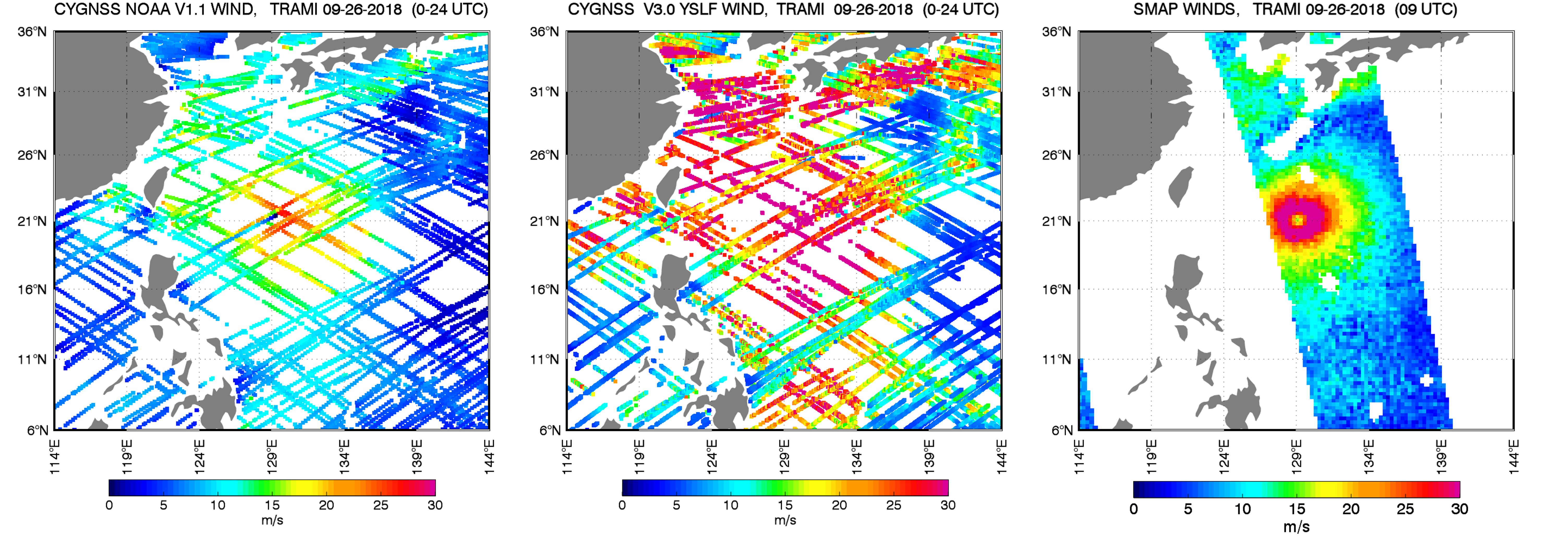
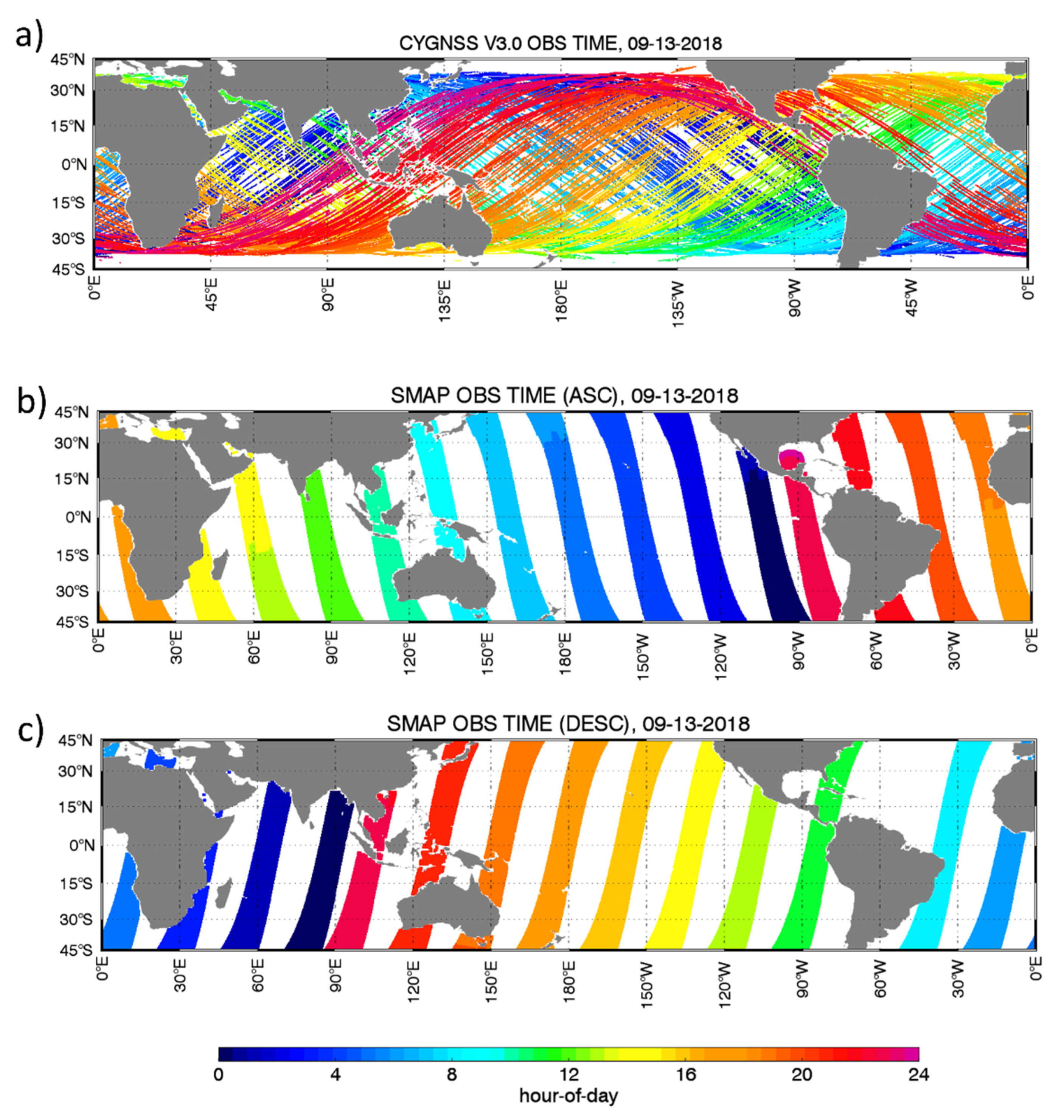
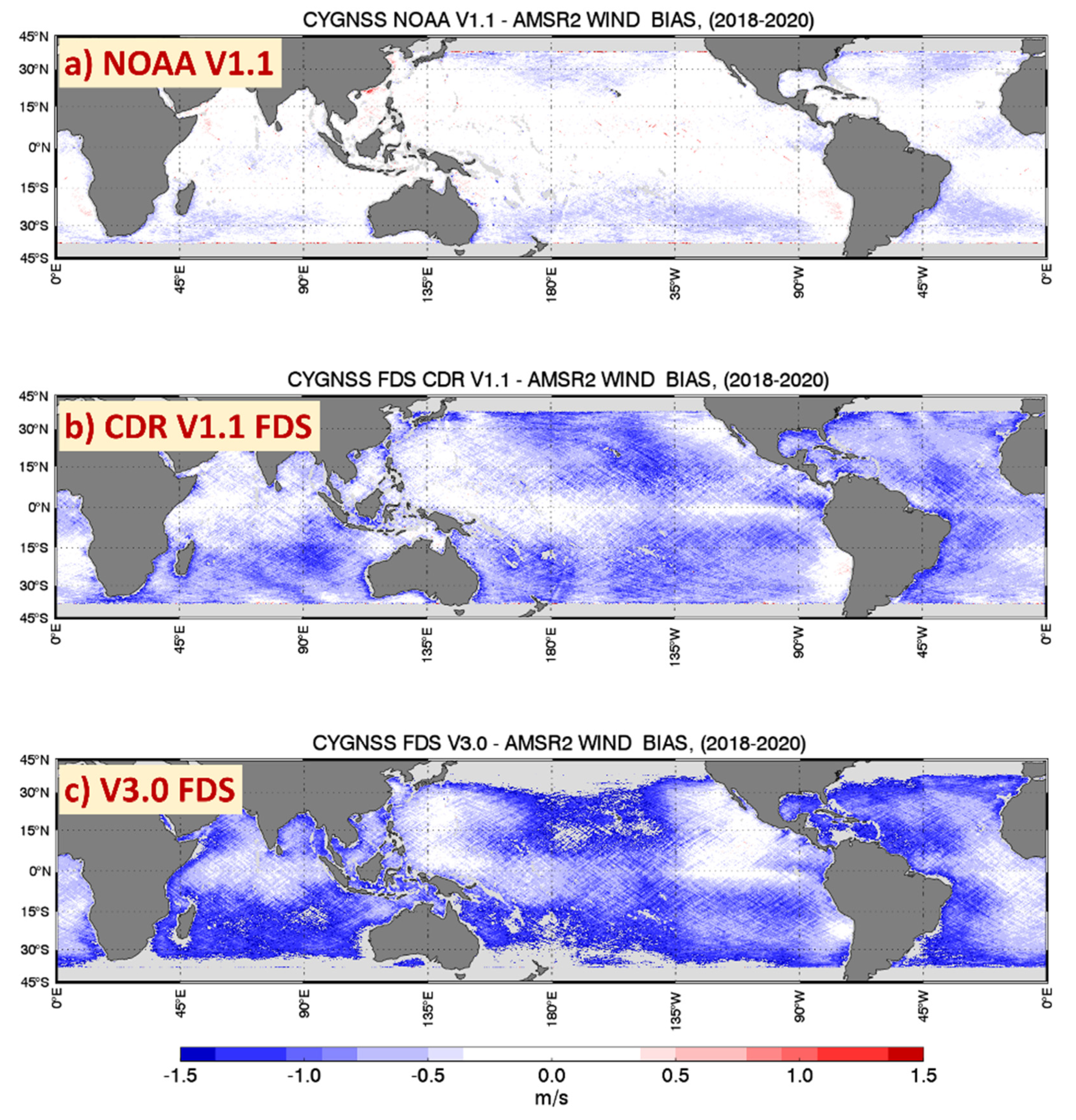
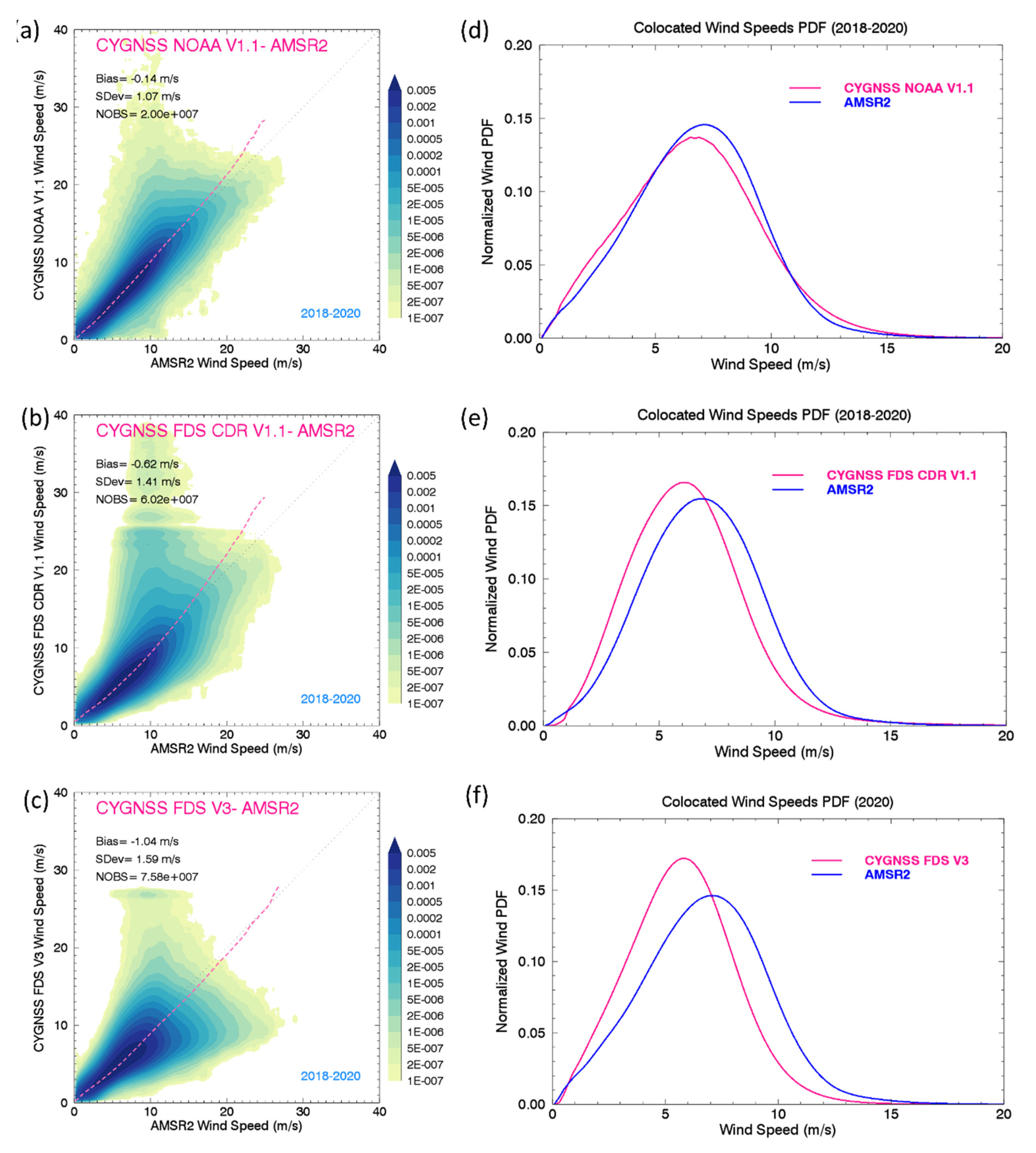
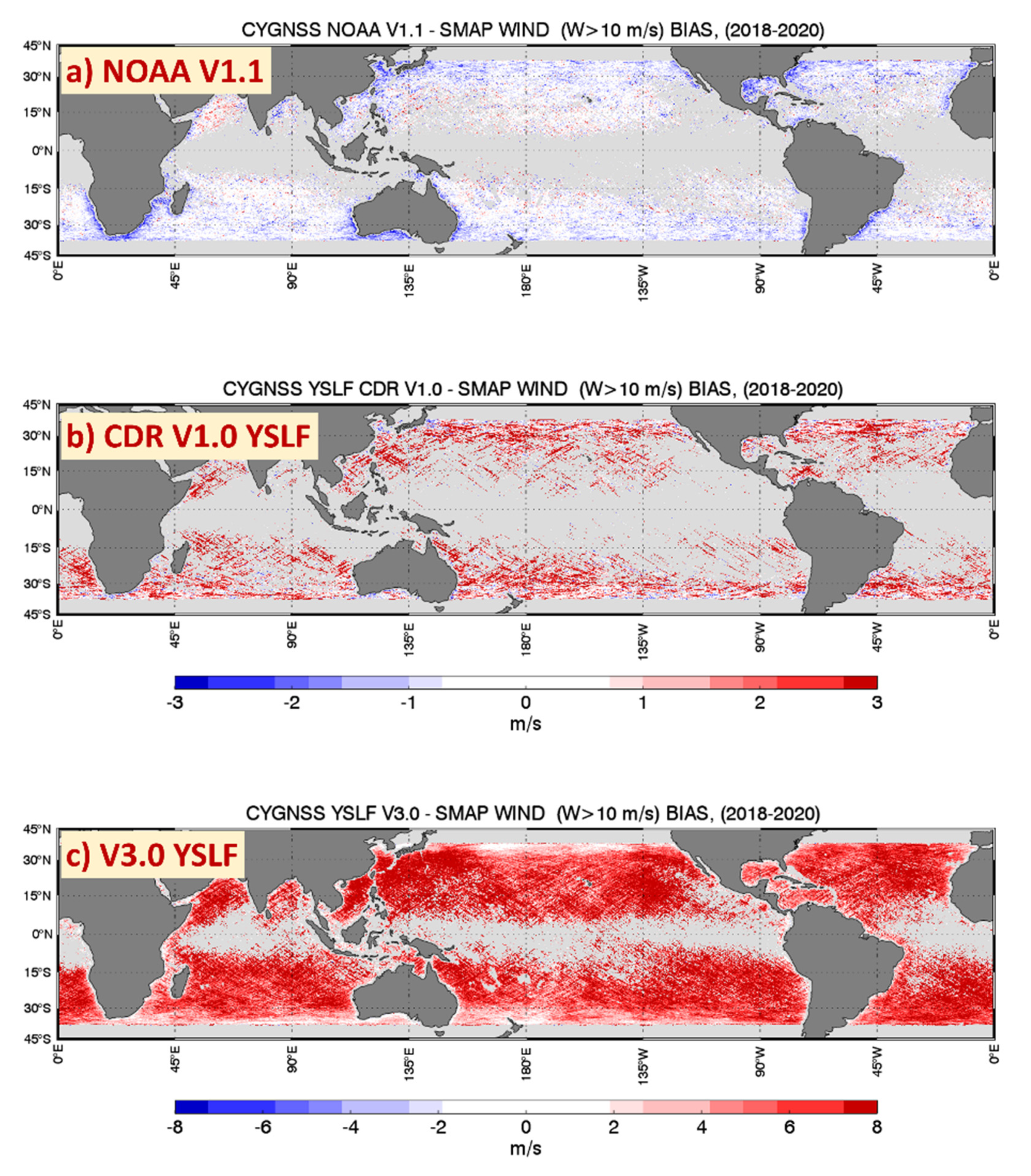
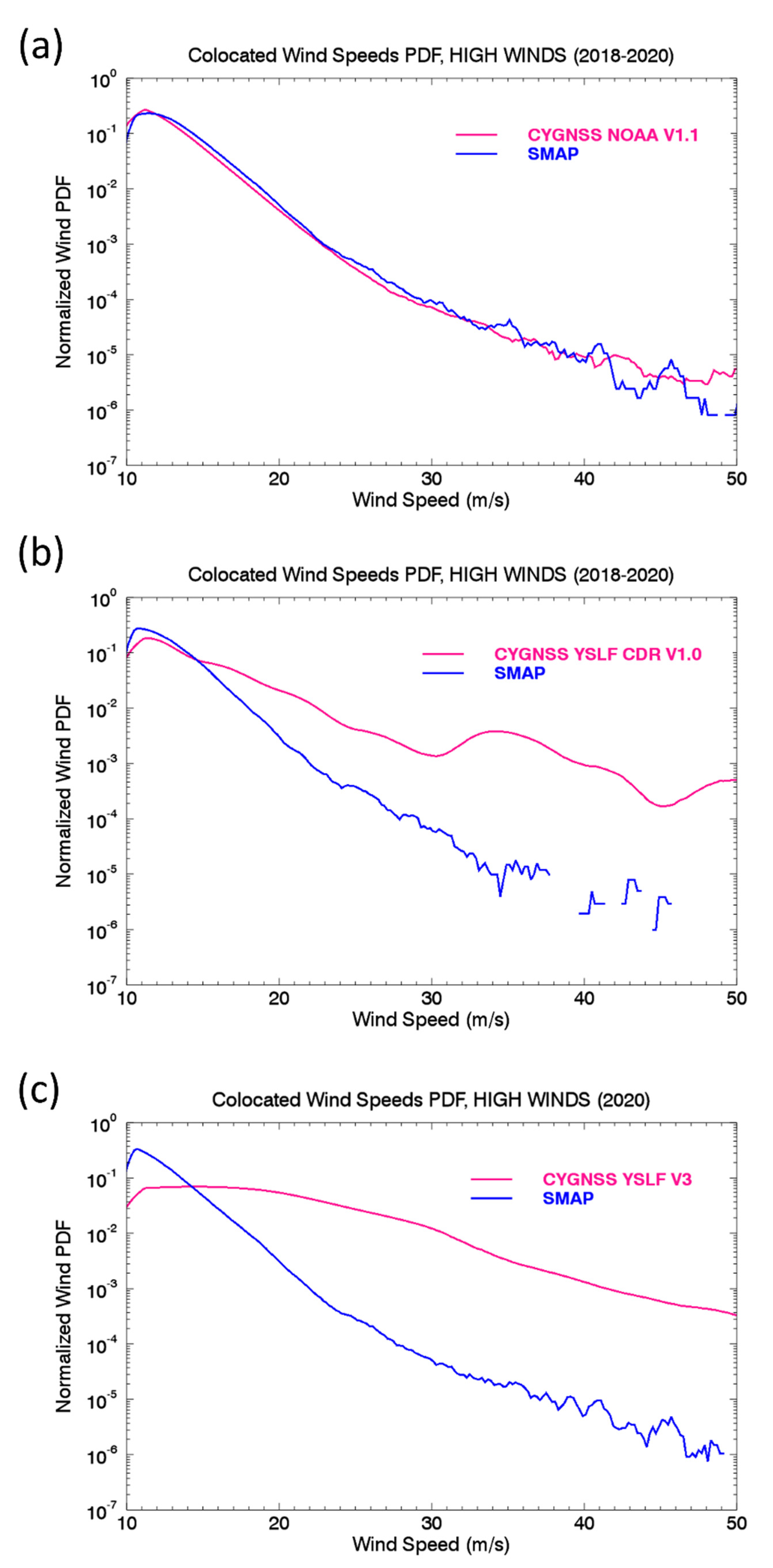
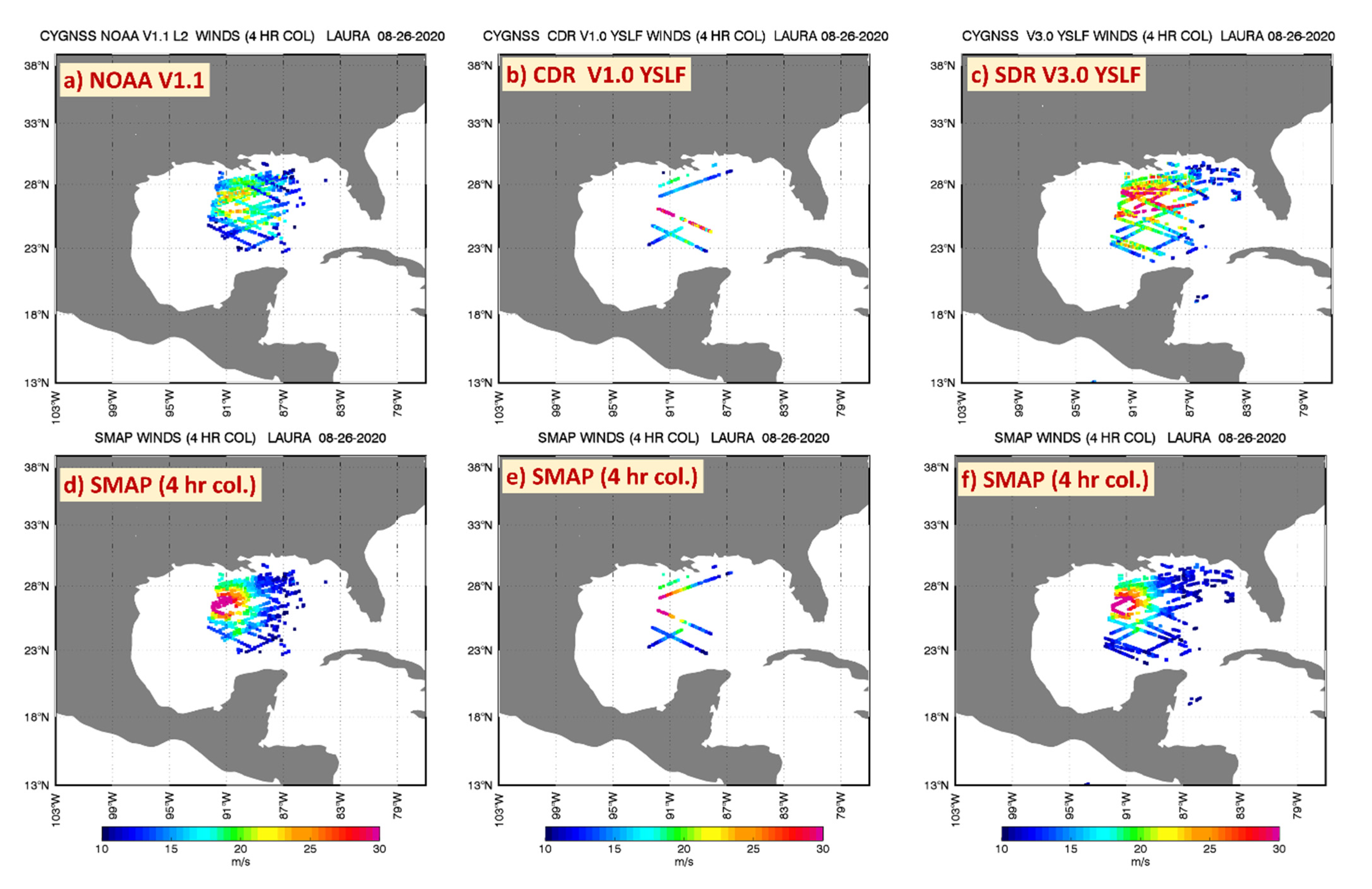
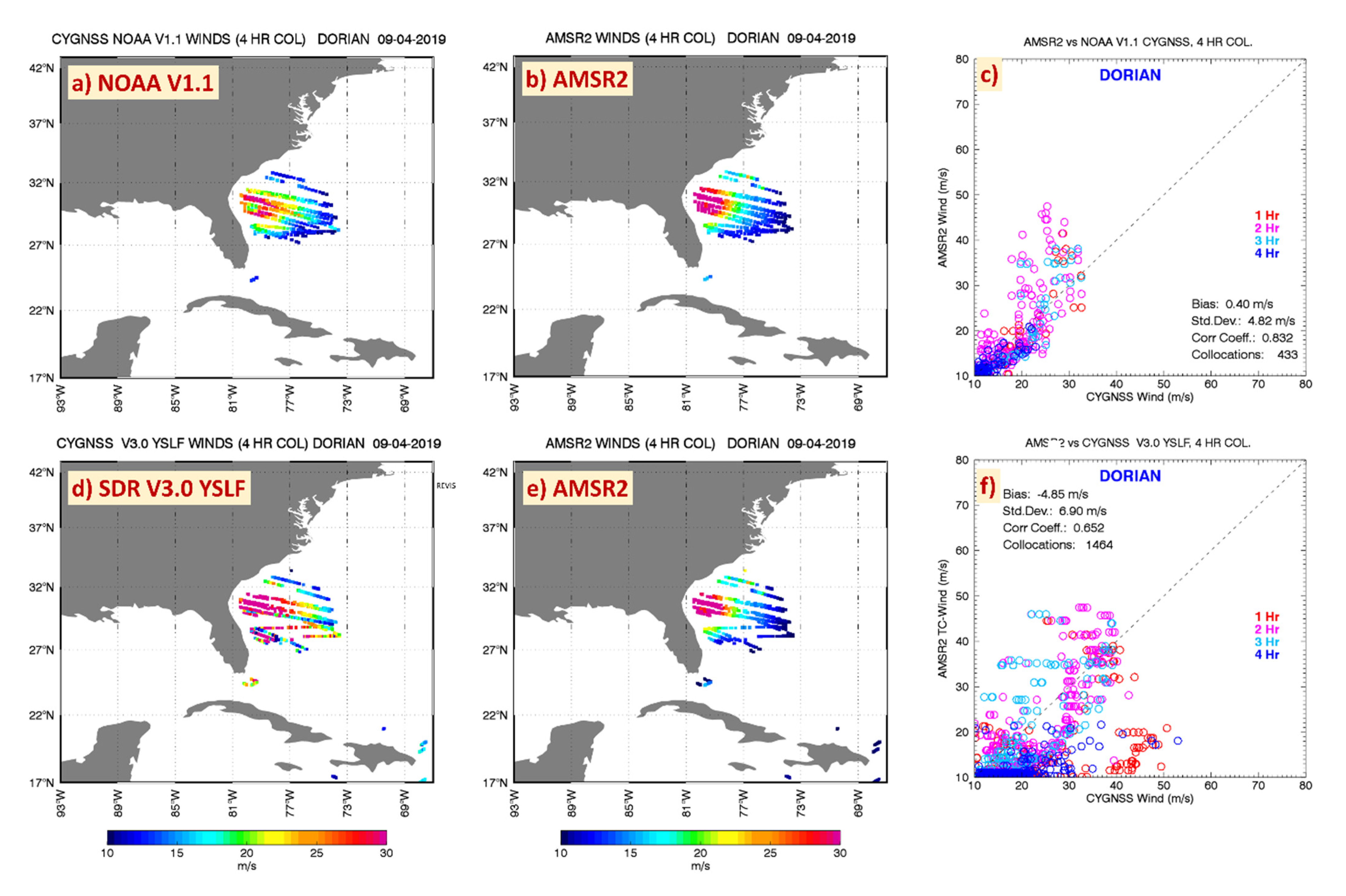
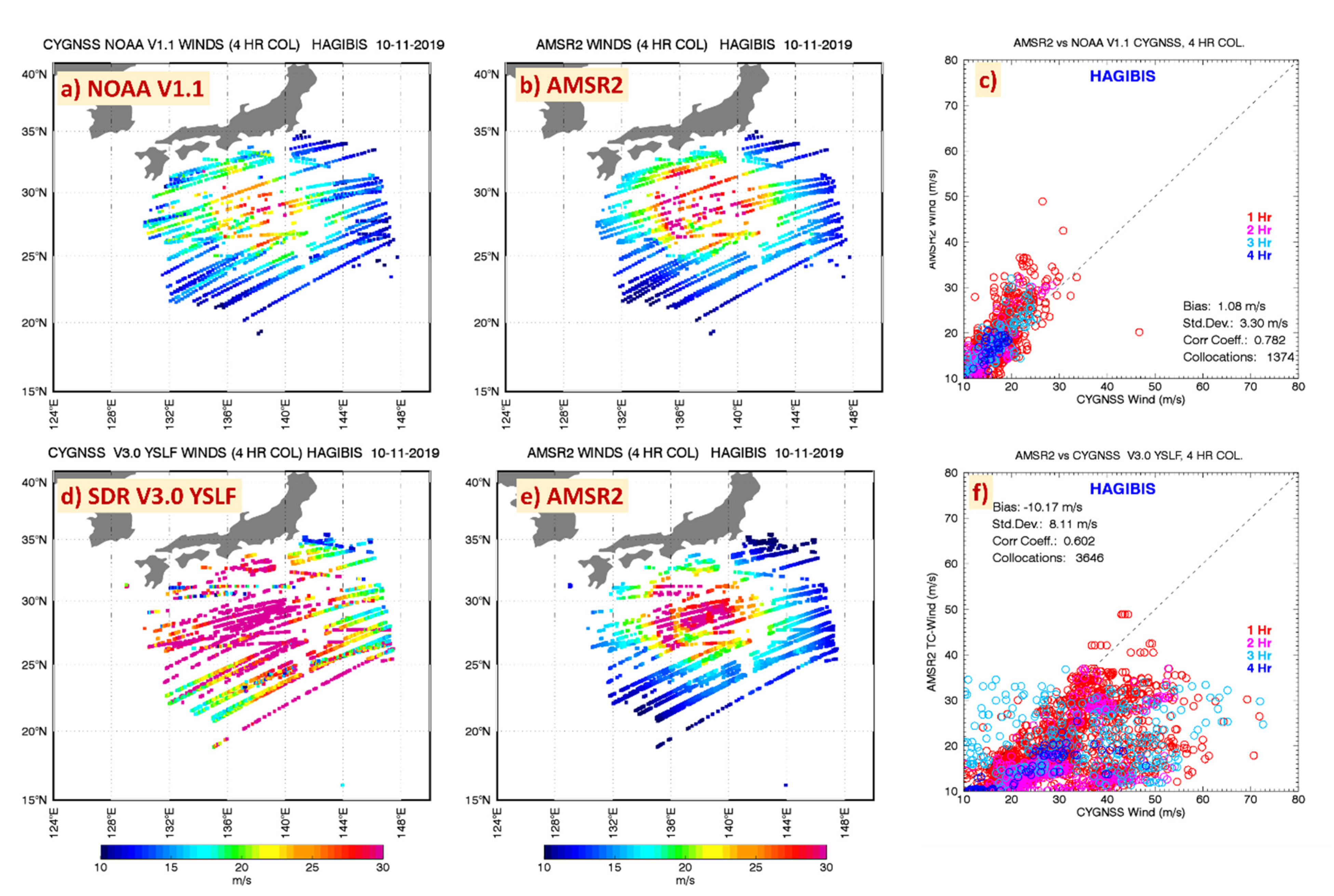
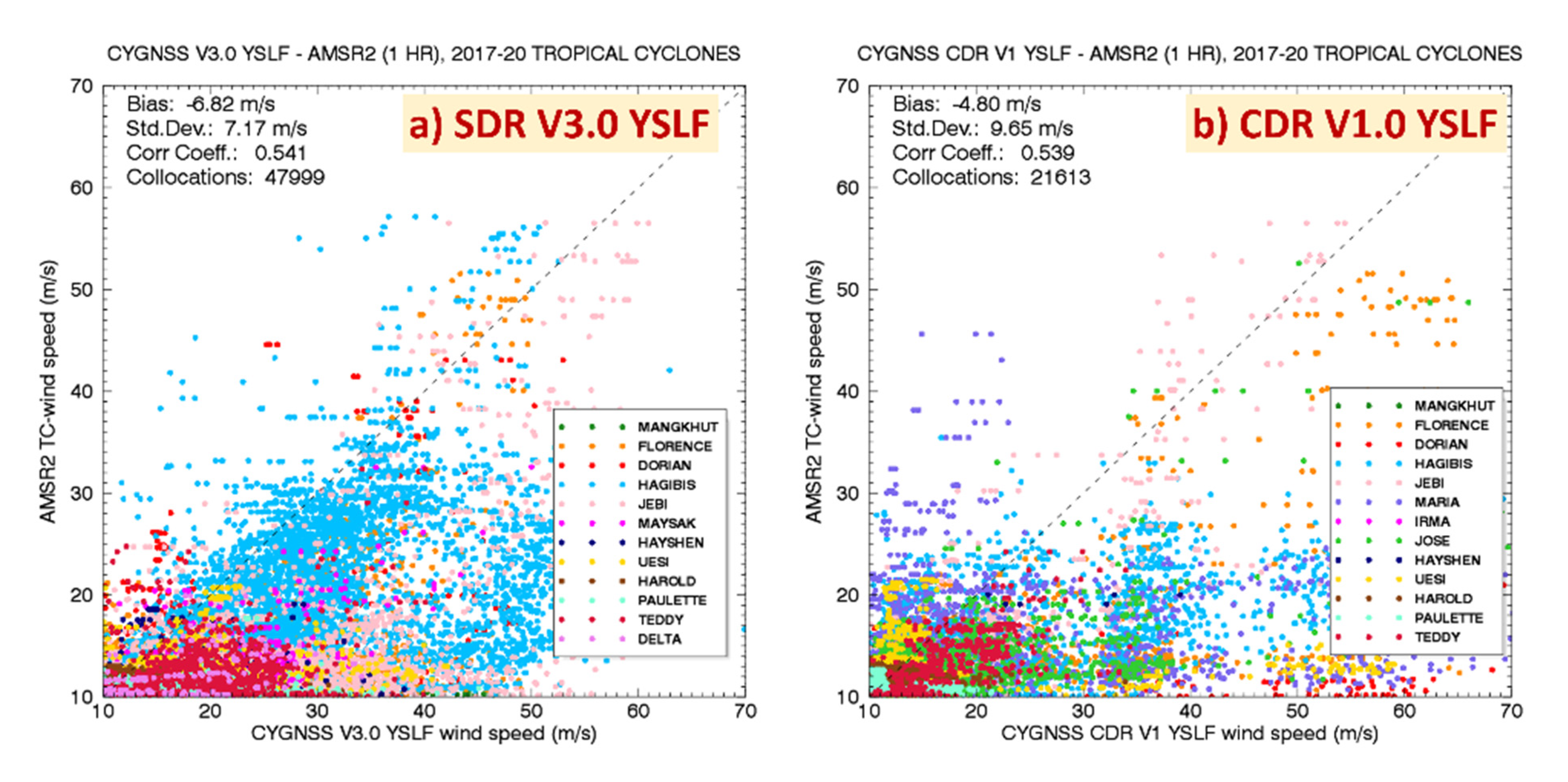
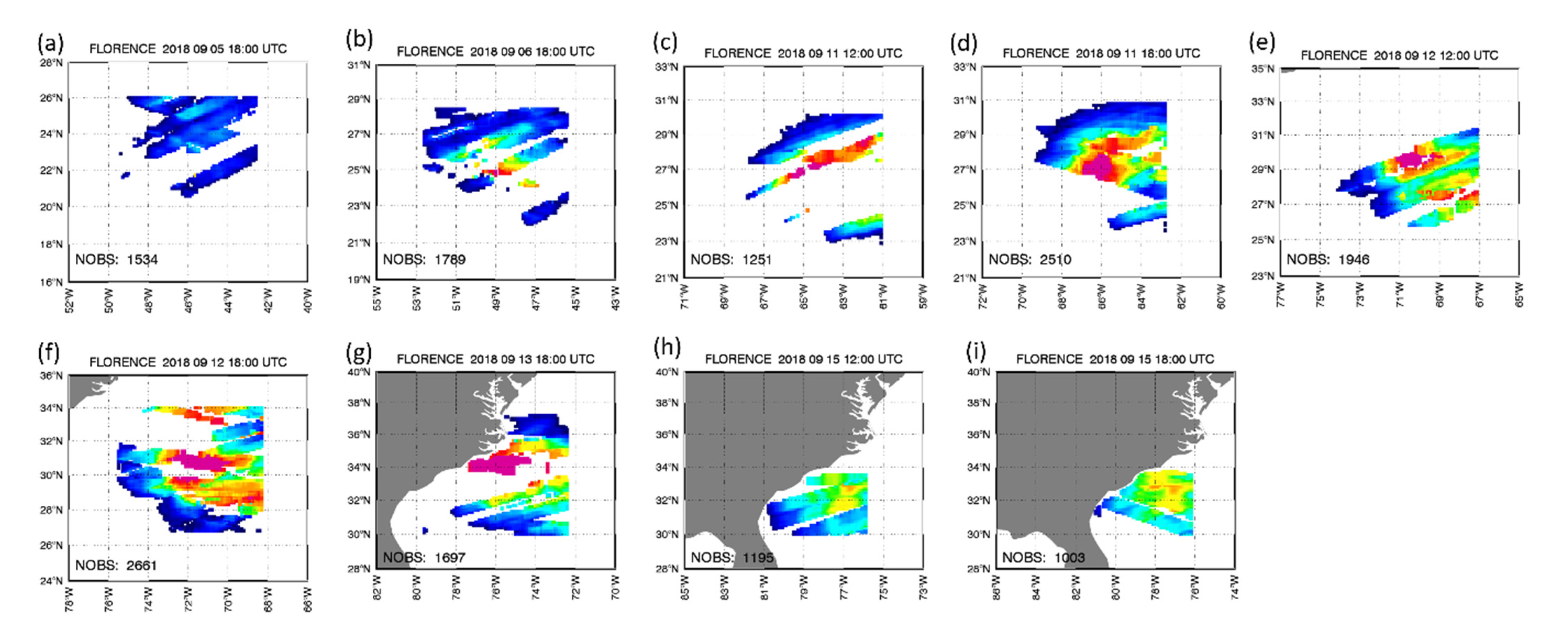
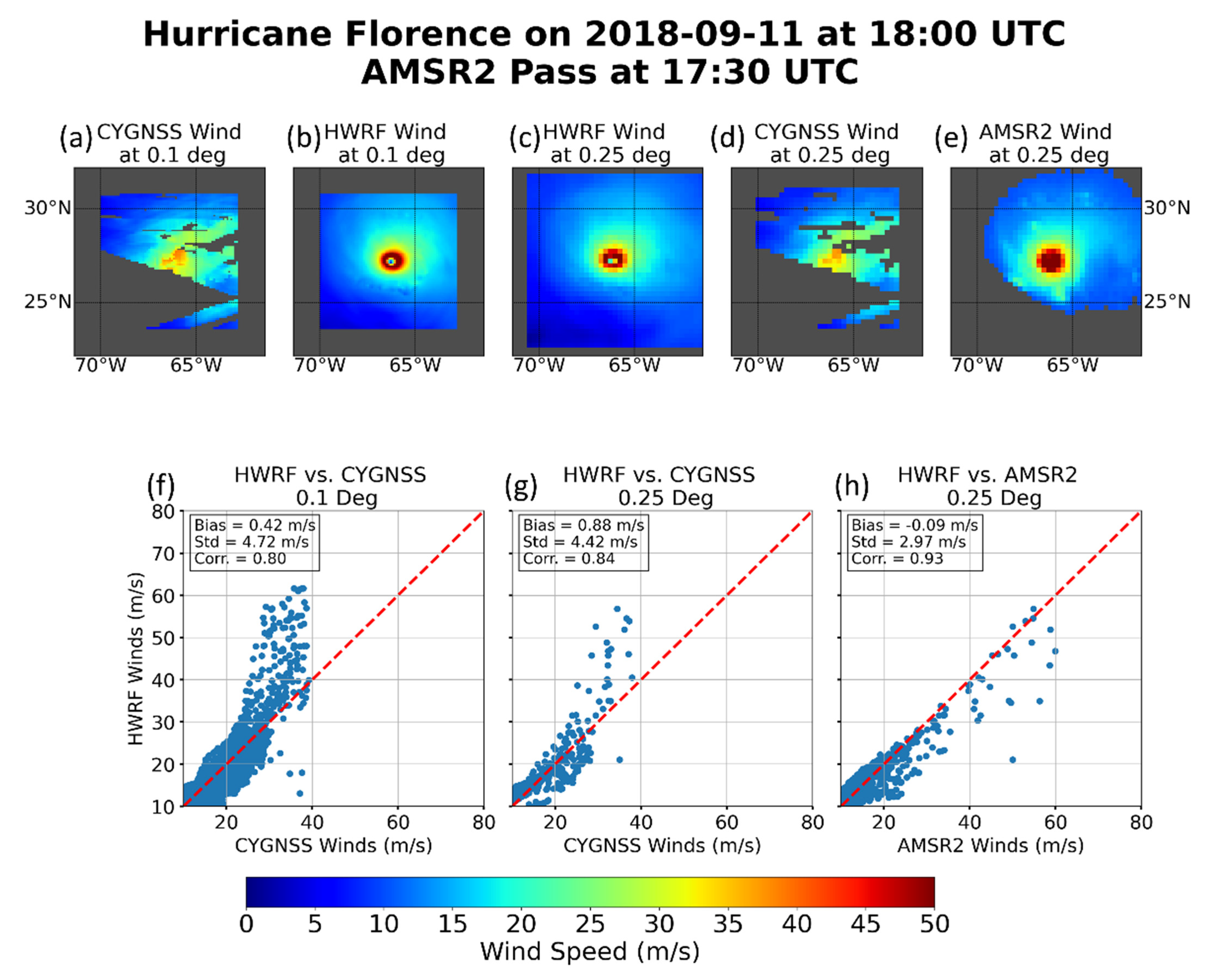
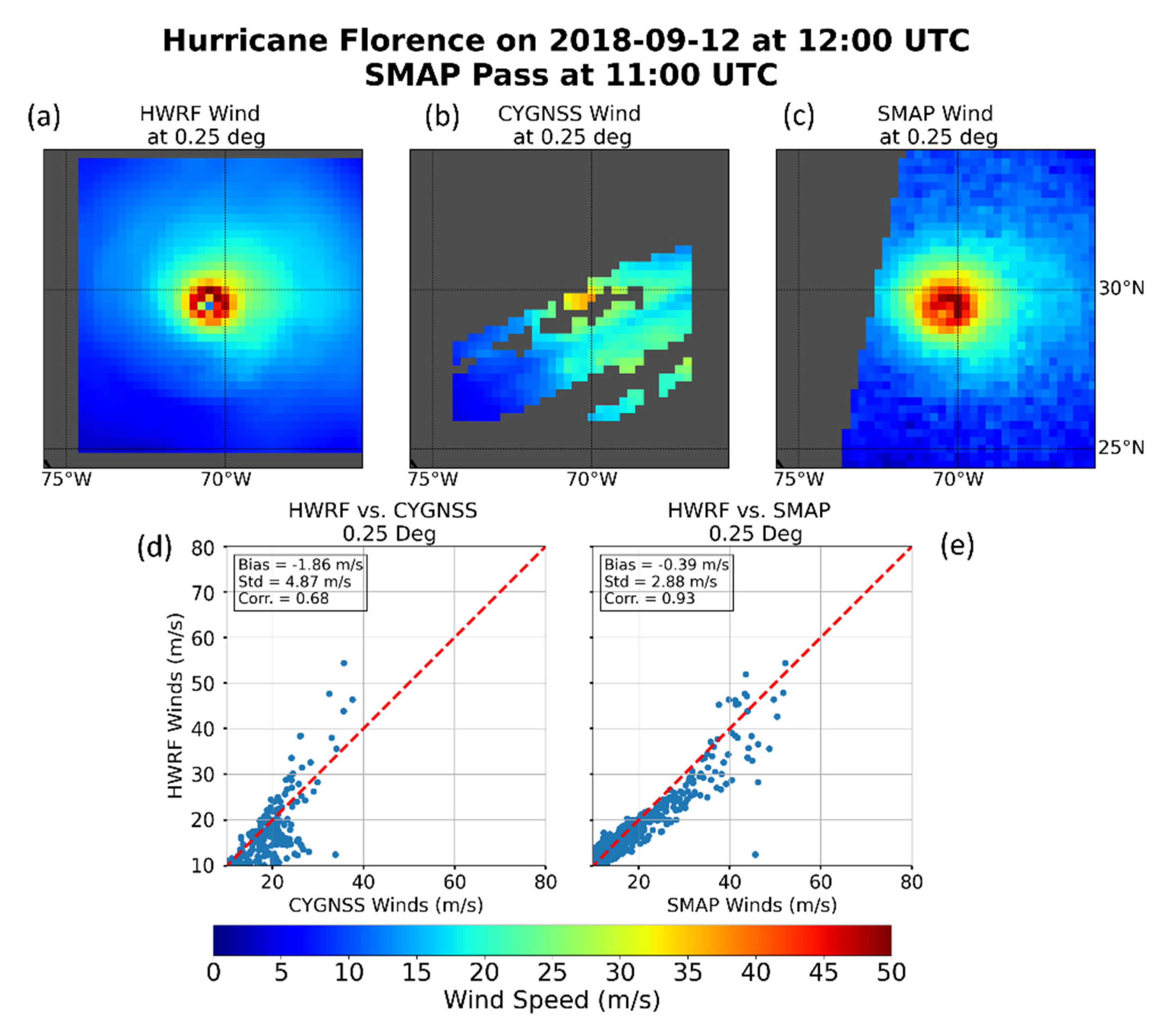
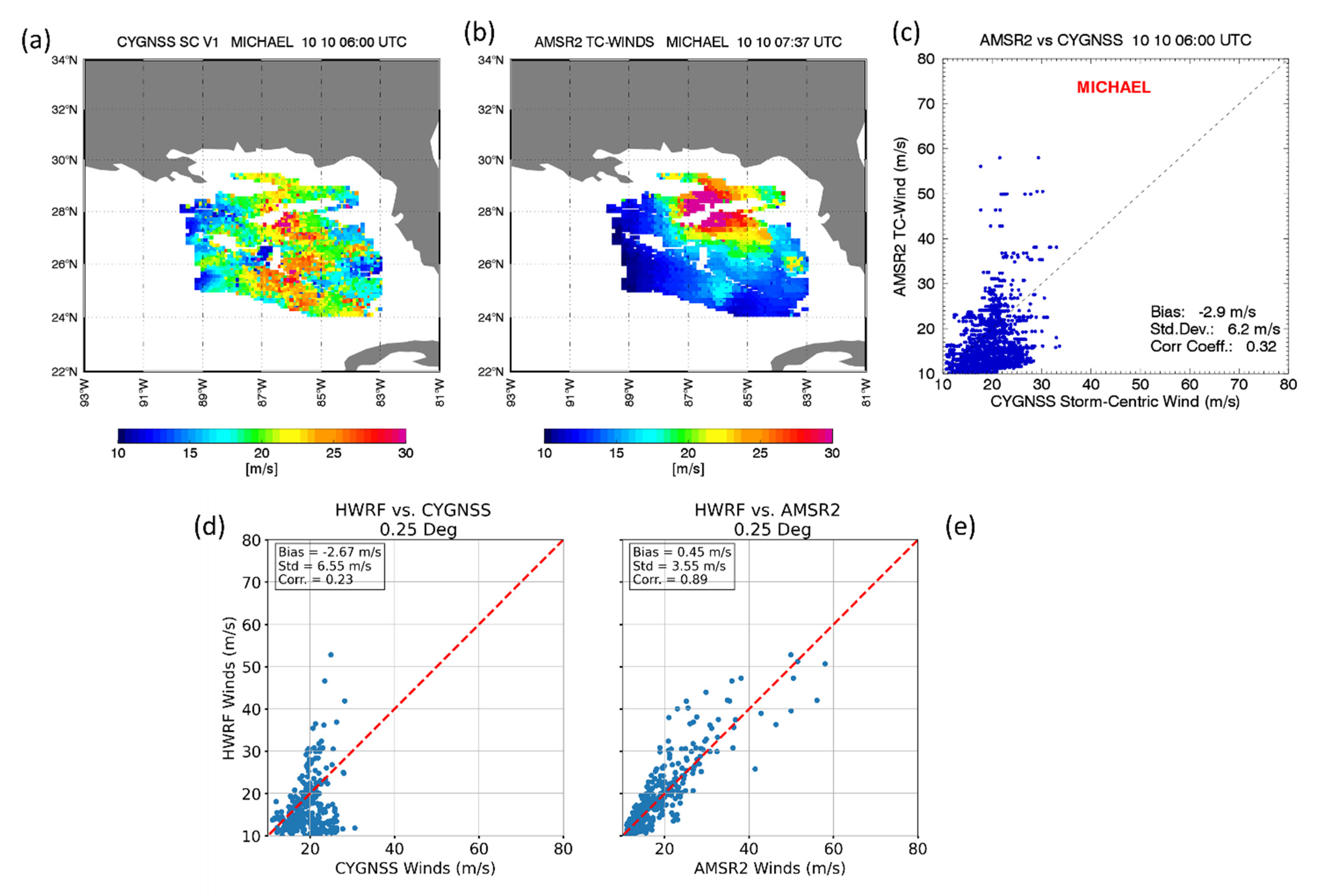
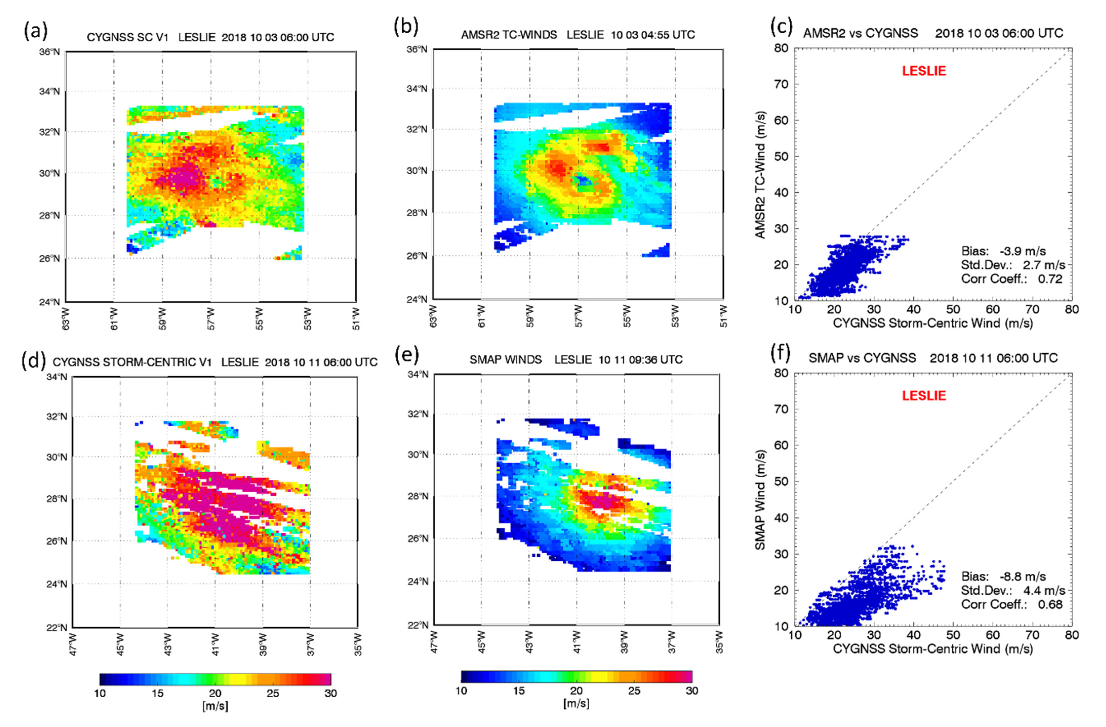
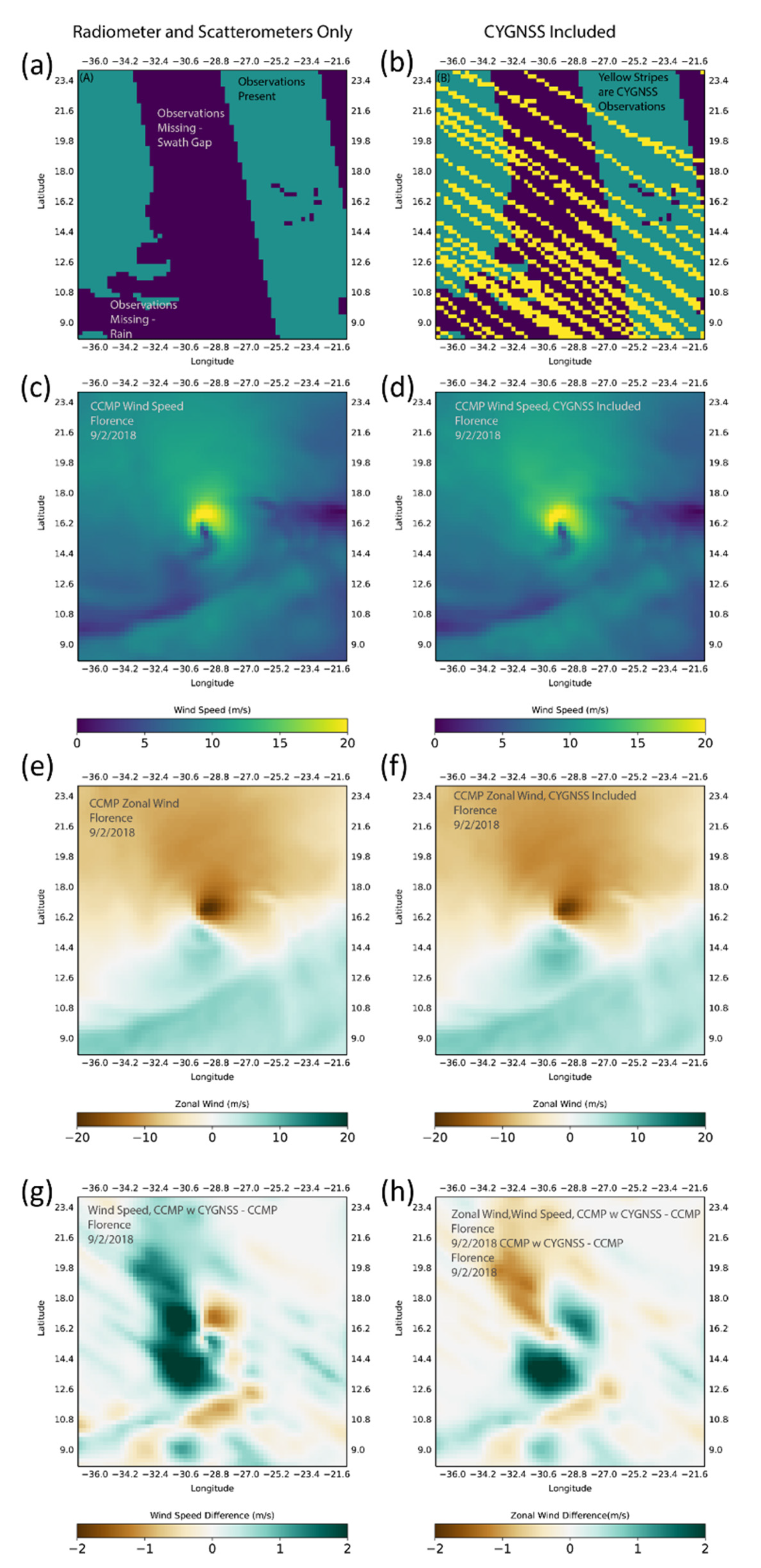
Table 1.
(a) Level 2 (L2) CYGNSS datasets assessed in this manuscript, all available on PO.DAAC, with the exception of NOAA V1.0, a preliminary beta version. (b) Level 3 (L3) CYGNSS datasets assessed in this manuscript, available on PO.DAAC. Notice that some datasets start in 2018 because they are processed using the V3.0 L1 files, which begin in 2018. Others (NOAA V1.1 and CDR V1.0) start in 2017 because they use V2.1 of L1 files, which are available from 2017 onward.
| (a) CYGNSS L2 | Start/End Date | Wind Products | Track-Wise Bias Correction (Dataset Used, Latency) |
| SDR V3.0 | Aug 2018–present | Fully Developed Sea (FDS) Young Sea Limited Fetch (YSLF) | No (~2 days) |
| CDR V1.0 | Mar 2017–Feb 2021 | FDS YSLF | Yes (MERRA2) |
| CDR V1.1 | Aug 2018–present | FDS only | Yes (MERRA2, ~1 month) |
| NOAA V1.0 (not on PO.DAAC) | 2017–2019 | Single wind algorithm, all winds | Yes (ECMWF) |
| NOAA V1.1 | May 2017–present | Single wind algorithm, all winds | Yes (ECMWF, ~6 days) |
| (b) CYGNSS L3 | Start/End Date | Wind products | Track-Wise Bias Correction (Dataset Used) |
| Storm-Centric | Aug 2018–Oct 2019 | Storm-centric, high winds only N. Atlantic and E. Pacific basins | No |
Publisher’s Note: MDPI stays neutral with regard to jurisdictional claims in published maps and institutional affiliations. |
© 2021 by the authors. Licensee MDPI, Basel, Switzerland. This article is an open access article distributed under the terms and conditions of the Creative Commons Attribution (CC BY) license (https://creativecommons.org/licenses/by/4.0/).
Share and Cite
MDPI and ACS Style
Ricciardulli, L.; Mears, C.; Manaster, A.; Meissner, T. Assessment of CYGNSS Wind Speed Retrievals in Tropical Cyclones. Remote Sens. 2021, 13, 5110. https://doi.org/10.3390/rs13245110
AMA Style
Ricciardulli L, Mears C, Manaster A, Meissner T. Assessment of CYGNSS Wind Speed Retrievals in Tropical Cyclones. Remote Sensing. 2021; 13(24):5110. https://doi.org/10.3390/rs13245110
Chicago/Turabian StyleRicciardulli, Lucrezia, Carl Mears, Andrew Manaster, and Thomas Meissner. 2021. "Assessment of CYGNSS Wind Speed Retrievals in Tropical Cyclones" Remote Sensing 13, no. 24: 5110. https://doi.org/10.3390/rs13245110
Note that from the first issue of 2016, this journal uses article numbers instead of page numbers. See further details here.