
Disparity Estimation of High-Resolution Remote Sensing Images with Dual-Scale Matching Network


1
State Key Laboratory of Information Engineering in Surveying, Mapping and Remote Sensing, Wuhan University, Wuhan 430079, China
2
School of Computer Science, China University of Geosciences, Wuhan 430074, China
3
Collaborative Innovation Center of Geospatial Technology, Wuhan University, Wuhan 430079, China
*
Author to whom correspondence should be addressed.
Remote Sens. 2021, 13(24), 5050; https://doi.org/10.3390/rs13245050
Submission received: 12 October 2021
/
Revised: 29 November 2021
/
Accepted: 9 December 2021
/
Published: 13 December 2021
(This article belongs to the Topic High-Resolution Earth Observation Systems, Technologies, and Applications)
Abstract
:As an essential task in remote sensing, disparity estimation of high-resolution stereo images is still confronted with intractable problems due to extremely complex scenes and dynamically changing disparities. Especially in areas containing texture-less regions, repetitive patterns, disparity discontinuities, and occlusions, stereo matching is difficult. Recently, convolutional neural networks have provided a new paradigm for disparity estimation, but it is difficult for current models to consider both accuracy and speed. This paper proposes a novel end-to-end network to overcome the aforementioned obstacles. The proposed network learns stereo matching at dual scales, in which the low one captures coarse-grained information while the high one captures fine-grained information, helpful for matching structures of different scales. Moreiver, we construct cost volumes from negative to positive values to make the network work well for both negative and nonnegative disparities since the disparity varies dramatically in remote sensing stereo images. A 3D encoder-decoder module formed by factorized 3D convolutions is introduced to adaptively learn cost aggregation, which is of high efficiency and able to alleviate the edge-fattening issue at disparity discontinuities and approximate the matching of occlusions. Besides, we use a refinement module that brings in shallow features as guidance to attain high-quality full-resolution disparity maps. The proposed network is compared with several typical models. Experimental results on a challenging dataset demonstrate that our network shows powerful learning and generalization abilities. It achieves convincing performance on both accuracy and efficiency, and improvements of stereo matching in these challenging areas are noteworthy.

1. Introduction
Disparity estimation from a pair of high-resolution remote sensing stereo images is a fundamental yet challenging task. It provides indepth information that is significant for scene understanding, height calculation, 3D reconstruction, to name a few [1]. As the data volume and application of remote sensing images grow rapidly, more stringent requirements are being imposed on the disparity estimation of remote sensing images.
Given a pair of rectified stereo images, the goal of disparity estimation is to match corresponding pixels on the left and right images and then compute a disparity map referring to the horizontal displacements. Disparity estimation has been intensively investigated for decades. Traditional algorithms [2,3,4,5] tackle this problem by adopting the classical four-step pipeline, including matching cost computation, cost aggregation, disparity calculation, and disparity refinement [6]. They compute the matching cost within a finite window and adopt hand-crafted schemes for the subsequent steps. Though significant progress has been made, they still have the limitation of dealing with texture-less regions, repeating textures, and occlusions. The accuracy and speed of traditional methods are unable to meet the actual application requirements in remote sensing.
Due to the powerful representative capability of convolutional neural networks (CNNs) and their success in various vision tasks [7,8,9,10], learning-based stereo methods have been employed to overcome the limitation of traditional methods in recent years. For example, MC-CNN [11] first introduces CNNs to calculate the matching cost by comparing image patches and proves the great potential of CNNs. Following it, several methods [12,13] are proposed to learn more efficient and robust matching cost computation. Besides, researchers also employ CNNs for cost aggregation [14,15] and disparity refinement [16,17]. These methods outperform traditional algorithms by applying CNNs to learn individual steps of the four-step pipeline [18]. However, hand-designed schemes are still required. Moreover, they are usually time-consuming, for multiple forward passes have to be conducted to calculate the matching cost of all potential disparities, and post-processing is required to refine the disparity [19]. This makes them not suitable for large-volume remote sensing images.
More recently, end-to-end networks have achieved unprecedented progress by integrating all steps into a whole network and directly predicting disparity maps from stereo pairs, driving disparity estimation towards a new paradigm. The milestone work is DispNet-C [20], which achieves comparable accuracy with MC-CNN but runs much faster on GPUs. It utilizes an encoder-decoder architecture that extracts unary features from an image pair by 2D CNNs, correlates the features with a correlation layer [21] then restores the original resolution by consecutive deconvolutions. Another groundbreaking work is GC-Net [22], which outperforms MC-CNN markedly but runs slower than DispNet-C. Instead of simply correlating features, GC-Net correlates features at all disparity levels by concatenating the left and right features to build a 4D cost volume and aggregates the cost by 3D CNNs. Besides, a differentiable soft argmin operation is proposed to regress continuous disparity values with sub-pixel accuracy. Following the two creative works, many studies [19,23,24,25,26,27,28,29,30] are conducted and attain further progress, dominating commonly used benchmarks such as KITTI [31,32], Middlebury [33], SceneFlow [20,34], etc.
Since end-to-end networks show superior performance in such public benchmarks, it is natural to consider employing them for remote sensing images. Ref. [35] first explores applying MT-CNN, DispNet-C, and GC-Net to a remote sensing dataset. As expected, GC-Net outperforms traditional algorithms and achieves the best accuracy among the three. However, the improvement is limited and the speed is unsatisfactory. We notice that compared with natural images, remote sensing images are more complicated despite the growing resolution, making the stereo matching more difficult. Firstly, there exist numerous regions with texture-less or repetitive patterns and complex structures. Secondly, disparities in remote sensing stereo images contain both negative and nonnegative values owing to significantly different viewing angles [36]. Thirdly, disparity discontinuities and occlusions are severe in certain areas because of large buildings and other tall objects. Moreover, the large size and huge amount of remote sensing images demand stereo matching algorithms with high efficiency and good generalization. To overcome these obstacles and further promote the performance of end-to-end networks, in this paper, we propose a brand-new CNN named dual-scale matching network (called DSM-Net for short) that mainly focuses on the following improvements.
- Our network learns stereo matching at both low and high scales, helpful for disparity estimation in large areas with texture-less and repeating patterns, as well as maintenance of main structures and details.
- We construct cost volumes from negative to positive values [36], making our network able to regress both negative and nonnegative disparities for remote sensing images.
- A 3D encoder-decoder module built by factorized 3D convolutions [37] is developed for cost aggregation, which can improve the stereo matching at disparity discontinuities and occlusions. Compared with standard 3D CNNs, the computational cost is markedly reduced.
- We employ a refinement module that ensures the network outputs high-quality full-resolution disparity maps.
On this basis, DSM-Net has a powerful capability to handle intractable situations. We evaluate it on a large-scale challenging remote sensing stereo dataset, the experimental results indicate that the proposed network achieves compelling disparity estimation accuracy while running at a decent rate.
2. Related Work
There exists a large body of literature on disparity estimation, we hereby review some typical end-to-end stereo matching networks, as they are dominating the disparity estimation domain and have enlightened our work. These networks can be broadly categorized into two distinct classes, 2D architectures and 3D architectures [18].
2D architectures. These architectures usually deploy an encoder-decoder design and adopt the general flow: the encoder extracts deep features from the input stereo pair, then a correlation layer encodes similarity into feature channels by computing the inner product of the left and right feature vectors along spatial and disparity dimensions, forming a 3D cost volume [21], which is finally parsed to disparity map by the decoder. The pioneering network is DispNet-C [20]. Following it, CRL [23] proposes a two-stage network that combines a DispNet-C model with a second sub-network for cascade learning of the disparity residual. iResNet [19] produces an initial disparity estimation, then iteratively refines it using multiple feature correlation and reconstruction error. MADNet [24] applies a coarse-to-fine strategy, starting from a coarser level of features to predict an initial disparity map then up-sampling it to a finer level with the assistance of warping operations. AANet [25] learns stereo matching on three scales, with an adaptive aggregation module for interaction among the different scales. Our network shares a similar idea with AANet, but we regress disparity maps from low scale to high scale in a coarse-to-fine manner, while AANet regresses that of three scales in parallel. These architectures run efficiently thanks to the efficiency of 2D convolution operations on modern GPUs. However, their accuracy is inferior to 3D architectures.
3D architectures. These architectures follow a similar flow to the former category. Differently, they encode similarity by computing the difference of left and right feature vectors [27,29] or directly concatenating them [22,26,28] to form a 4D cost volume, then the 4D tensor is processed by 3D convolutions. GC-Net [22] is the first attempt. Following this new design, PSMNet [26] utilizes spatial pyramid pooling layers (SPP) [38] in its feature extractor to integrate features with multiple scales and deploys a stack of 3D hourglass modules to learn cost volume regularizing. ECA [28] introduces an explicit cost aggregation module to improve the 3D optimization by using a 3D encoder-decoder module. StereoDRNet [29] applies 3D dilated convolutions inside its stacked encoder-decoders to further improve the effectiveness and add a refinement sub-network for enhancing the disparity map. Due to that real geometric context [22] can be explicitly learned by 3D convolutions, 3D architectures achieve better accuracy than 2D architectures in most cases. However, 3D convolutions require higher computational effort owing to more parameters and floating-point operations (FLOPs). To make the model runs in real-time, StereoNet [27] constructs a low-resolution cost volume to produce a coarse prediction then hierarchically guide it to the original resolution with the (resized) left image. MABNet [30] proposes a multibranch adjustable bottleneck module that is less demanding on parameters to replace standard 3D convolutions, making the model lightweight. However, their accuracy decreases compared to the heavy models. We also explore how to make the model lightweight. In our network, we replace conventional 3D convolutions with efficient factorized 3D convolutions to reduce the computational burden.
Inspired by these methods and aimed at remote sensing images, we build DSM-Net, which belongs to the latter category and achieves high accuracy while maintaining a satisfactory speed.
3. Dual-Scale Matching Network
We first provide an overview of the proposed network, then introduce the components in detail, followed by the loss function used to train our network.
3.1. Overview
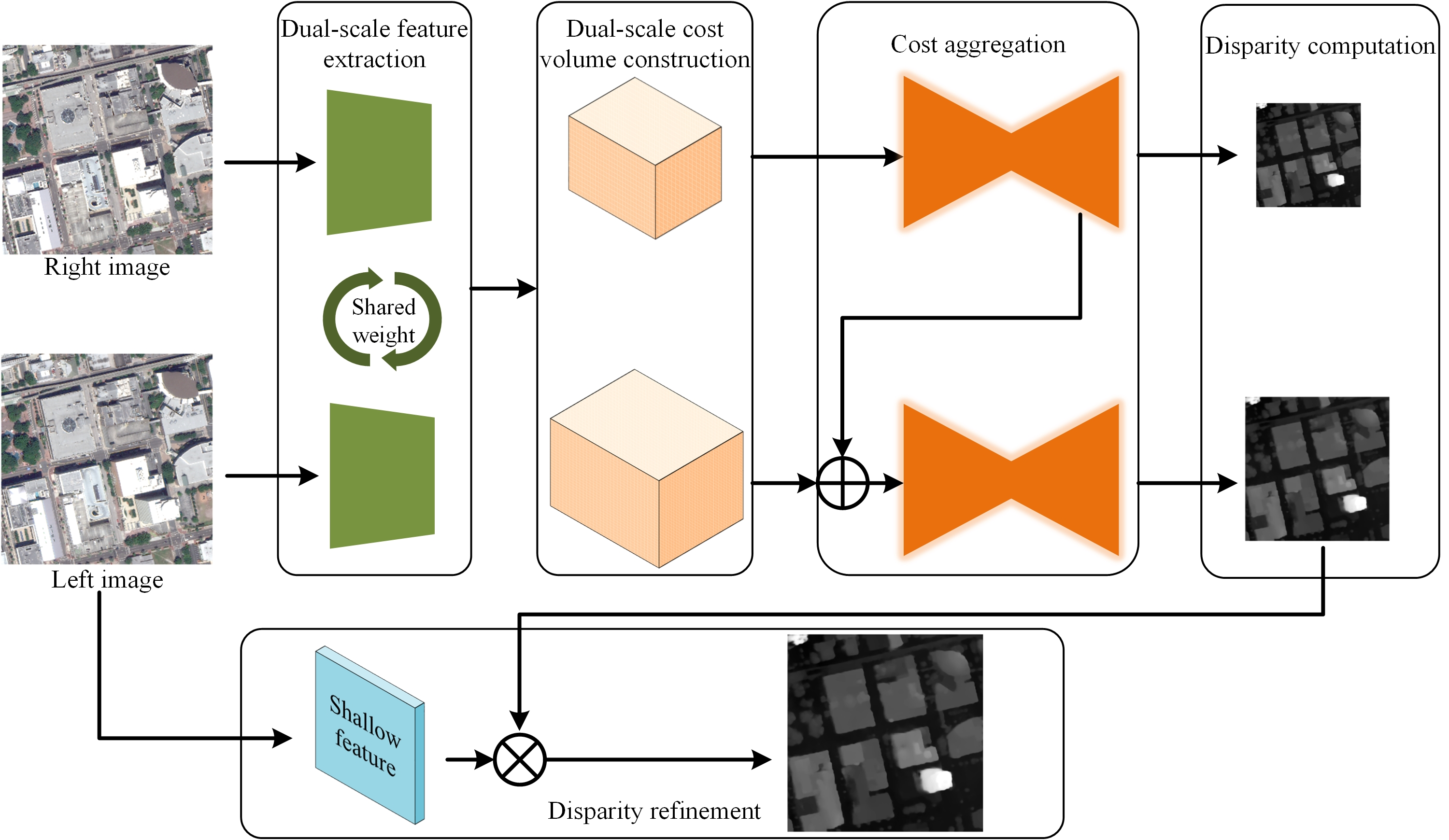
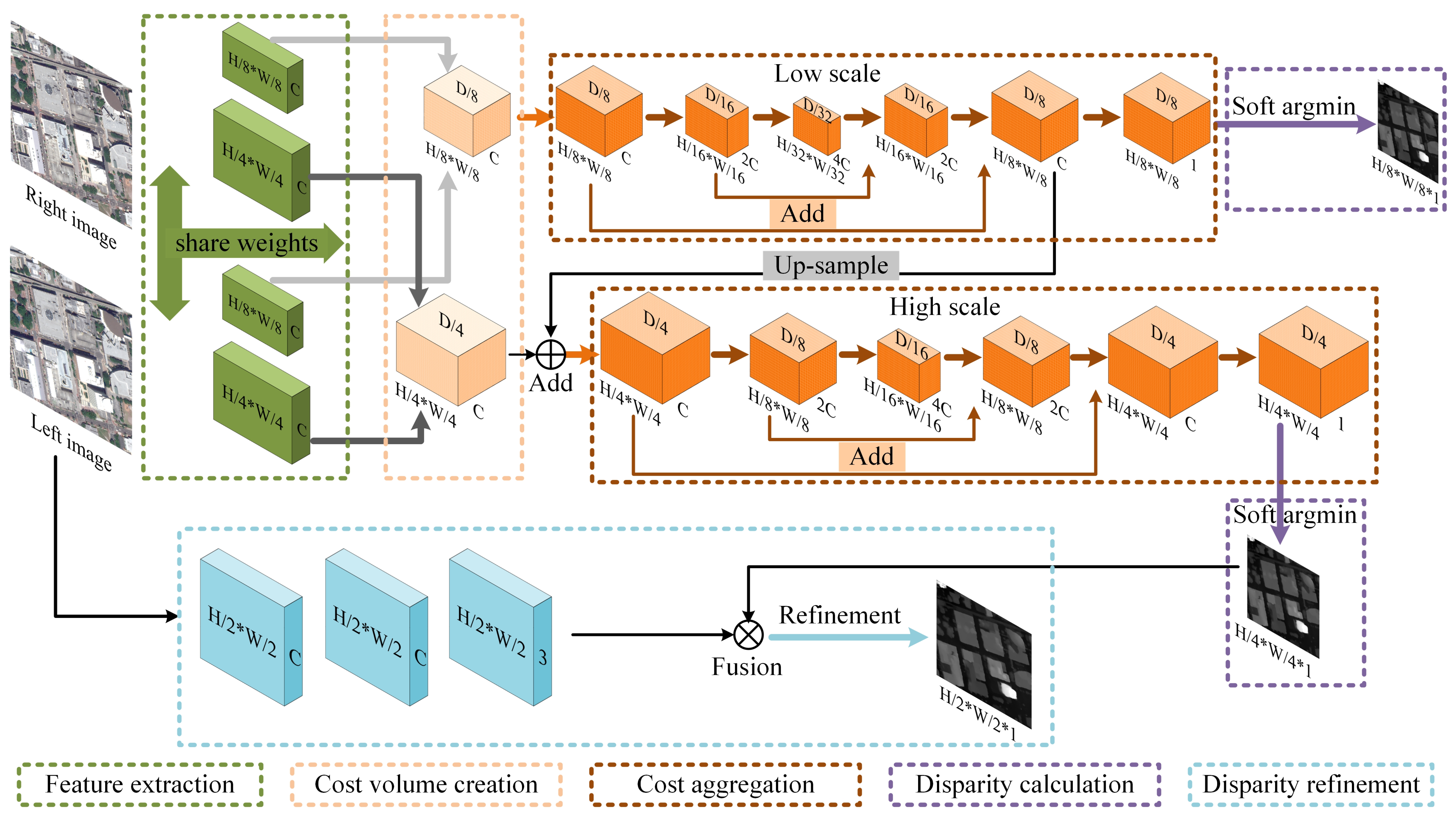
Given a rectified image pair, DSM-Net predicts the disparity map by executing the flow shown in Figure 1, which consists of five parts. We first extract down-sampled features at 1/4 and 1/8 resolutions with a shared 2D CNN. Then the dual-scale 4D cost volumes are created by conducting the difference operations [27,29] at corresponding scales. In the cost aggregation stage, we first use a 3D encoder-decoder module (roughly displayed in the figure, details will be introduced in the subsequent section) to aggregate the low-scale cost volume, then the last but one 4D volume is bilinearly up-sampled and added to the initial high-scale cost volume, which is aggregated by another 3D encoder-decoder module (same as the former one). Next, we adopt the soft argmin operations [22] to compute the disparity maps of 1/4 and 1/8 resolutions. Finally, the disparity refinement module takes as input the shallow features extracted from the left image and the disparity map regressed at the high scale, producing the refined disparity of 1/2 resolution, which is directly up-sampled to full resolution as the final prediction via bilinearity (not included in the figure).
3.2. Components
3.2.1. Feature Extraction
The first step is to find meaningful features that can effectually represent image patches. Remote sensing images contain objects of different scales, therefore, deep features are extracted at both the low and high scales. The low scale can capture coarse-grained information from low-resolution features using a larger receptive field, while the high scale can capture fine-grained information from high-resolution features with richer details. A 2D CNN with shared weights (also known as a Siamese network [39]) between the input image pair is used. The architecture is shown in Table 1. We first decimate the input resolution down to 1/4 of the original input size, then apply two branches to extract features of two scales respectively. Basic residual blocks [40] are used to boost the 2D CNN.
3.2.2. Cost Volume Creation
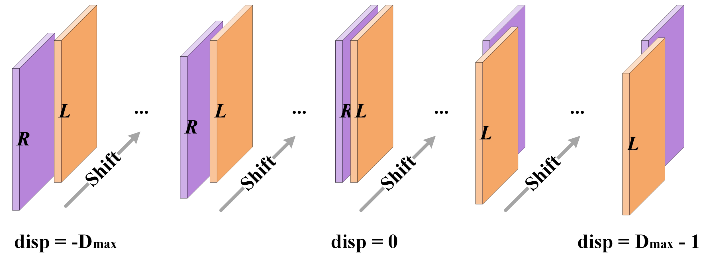
At this point, the dual-scale 4D cost volumes are created by taking the difference of the feature vector of a pixel and the feature vectors of the matching candidates at corresponding scales. Typical CNN-based methods would form a cost volume that only contains nonnegative values. However, remote sensing images may be collected at different times, and the viewing angles could be significantly different, thus both negative and nonnegative disparities appear in remote sensing stereo images even though they have been rectified. To make our network predict nonnegative as well as negative disparities, we build cost volumes covering the range [, ). Because the input images are rectified, disparity exists only in the horizontal direction. We can simply employ a shift operation to form a cost volume. The left feature is awaiting to be subtracted, and the right feature slides on the left feature horizontally, as depicted in Figure 2. After packing the subtraction results, we get a 4D volume with a shape of , where denotes the shape of left and right features and D denotes the disparity range.
3.2.3. Cost Aggregation
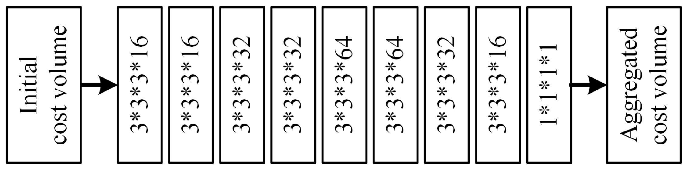
Cost aggregation can rectify the mismatching cost value computed from the local feature with large view guidance and ensure a high-quality disparity map with smoothness and continuity. 3D convolutions are effective to conduct cost aggregation along spatial and disparity dimensions as well as learn geometric context [22] but are also time-consuming. To reduce the computational burden, we factorize a standard 3D convolution into two stacked subcomponents, namely disparity-wise convolution, and spatial-wise convolution. The former has a kernel of and the latter has a kernel of . The stacked subcomponents play the same role as a standard 3D convolution but are much more efficient. Suppose that both the input and output have a shape of , the number of parameters in a standard 3D convolution (with a kernel size of and stride of 1) is , and the FLOPs is . However, these in a factorized 3D convolution are only and , respectively. Both the parameters and FLOPs are dramatically decreased.
To further increase the efficiency and make the aggregation module has a larger view, we adopt an encoder-decoder with skip connection design, which is similar to the explicit cost aggregation module in ECA [28], as illustrated in Figure 1 and Table 2. For one thing, the computational burden can be further reduced by subsampling and up-sampling operations. For another, the module acquires a larger receptive field due to down-sampled cost volume. Besides, skip summations from encoder to decoder help the module learn sufficient and multilevel geometric context. Moreover, to establish a connection between the dual scales during aggregation, we up-sample the last but one 4D volume in the low scale and add it to the initial high-scale cost volume. Because of the lower resolution, the disparity search range is smaller and the aggregation is easier at the low scale, which should be carried out first. We believe the coarse-to-fine manner makes the low scale servers as prior knowledge and provides beneficial guidance for the high scale.
3.2.4. Disparity Calculation
We adopt the differentiable soft argmin operation as proposed in GC-Net [22] to transform the aggregated cost volumes into continuous disparity maps, which can retain a sub-pixel accuracy. The matching cost value is first converted to probability value via a softmax function across the disparity dimension, then the final disparity is obtained by taking the sum of each disparity weighted by its probability. The mathematical equation is given by:
where and d refer to the predicted disparity and disparity candidate, and c refer to the softmax function and matching cost (for each disparity candidate), respectively.
3.2.5. Disparity Refinement
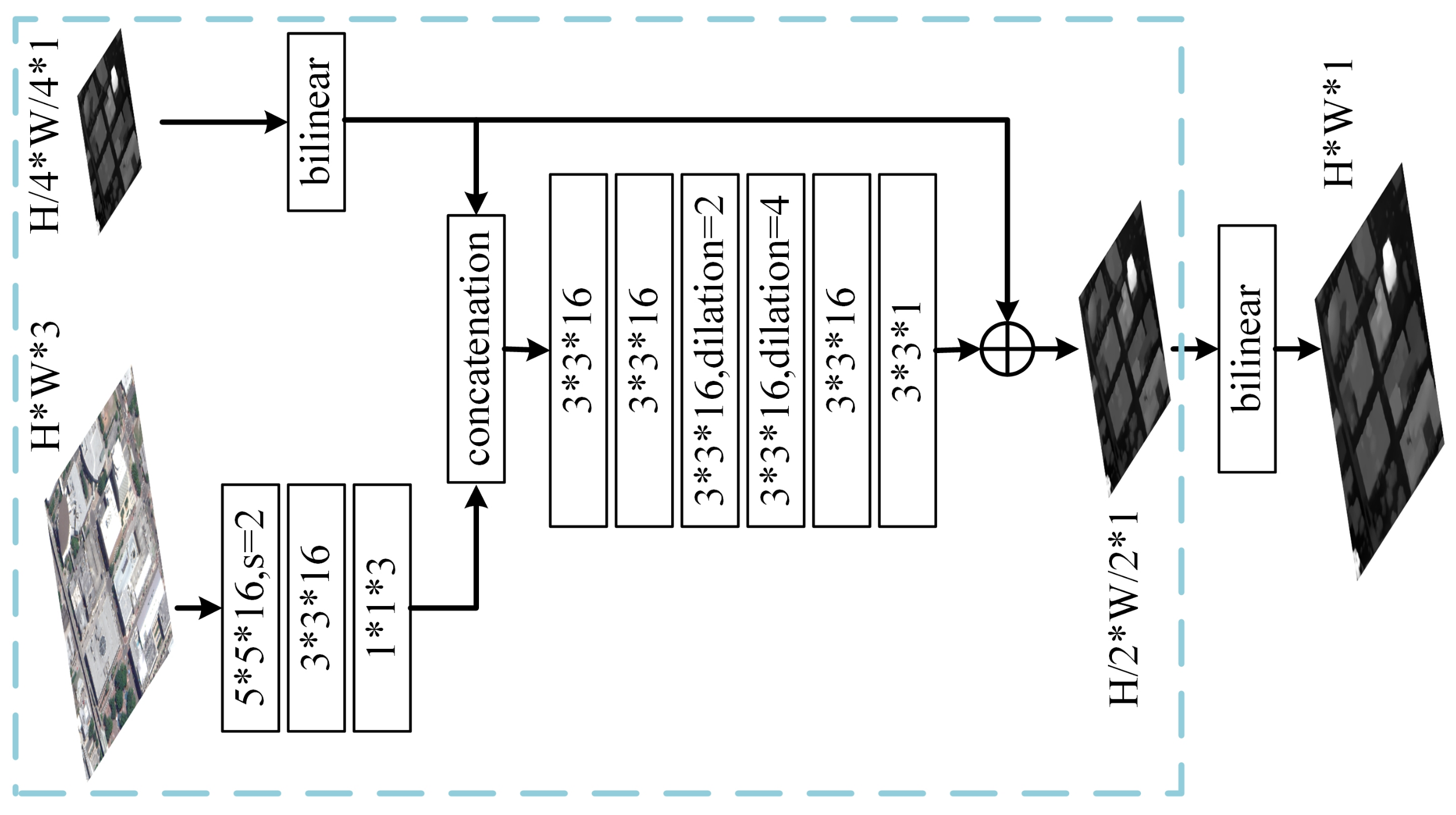
The output disparity maps are 1/8 and 1/4 resolution of the original image. If directly up-sampled to full resolution, mosaics would occur on the full-resolution disparity map. To attain high-quality full-resolution prediction as well as bring in more fine details and motivated by the refinement strategy in StereoNet [27], we utilize a refinement module that blends in high-frequency information as guidance. Our refinement module (depicted in Figure 3) first extracts shallow features that are robust to noise and luminance change [23] from the input left image, then concatenates them with the disparity map estimated by the high scale up-sampled to 1/2 resolution (in StereoNet, the resized input left image is directly concatenated with the low-resolution disparity map). The concatenation is processed by a stack of 2D convolution layers, producing a residual (also known as a delta disparity) that is next added to the up-sampled disparity map. Finally, the summed disparity map (regarded as refined disparity map) is directly up-sampled to full resolution as the ultimate prediction.
3.3. Loss Function
We train the proposed DSM-Net in a fully supervised manner using ground-truth-labeled stereo data, adopting the smooth L1 loss function that is robust and lowly sensitive to outliers [44]. The supervised loss is defined as:
in which:
where N is the valid number of labeled pixels, d and represent the ground-truth and predicted disparities. The supervision is conducted on the three disparity maps output by the low scale, high scale, and refinement module. Thus, the final loss function is the weighted summation of the three ones (note that the predicted disparity map is always bilinearly up-sampled to match the ground-truth resolution before loss computation):
where , , and are the loss weights.
4. Experiments
In this section, we first give a brief introduction to the dataset for approach evaluation and the metrics for quantitative assessment. Then, the implementation details of our network and several state-of-the-art methods used for comparison are described. Finally, we display the experimental results and analyze them.
4.1. Dataset and Metrics
We evaluate the performance of our method on the challenging US3D track-2 dataset of the 2019 Data Fusion Contest [45,46]. This dataset contains high-resolution multi-view images collected by WorldView-3 between 2014 and 2016 over Jacksonville and Omaha in America, covering various landscapes such as residential buildings, skyscrapers, rivers, woods, etc. Stereo pairs in this dataset are rectified in size 1024 × 1024 and geographically non-overlapped. Jacksonville and Omaha have 2139 and 2153 RGB image pairs with ground-truth disparity labels, respectively. We use image pairs from Jacksonville to train and test our model, while all image pairs from Omaha are used to evaluate the generalization ability of the proposed network. Table 3 shows the usage of the dataset.
Stereo performance is assessed in terms of both accuracy and efficiency. For accuracy assessment, we use the average endpoint error (known as EPE, the average absolute distance between estimated and ground-truth disparities) and the fraction of erroneous pixels (known as D1, a pixel is regarded erroneous if its predicted disparity has an absolute error larger than 3 pixels) as quantitative metrics. Note that only valid pixels are used to calculate the two metrics. For efficiency assessment, we compute the time required for a network to inference a disparity map from a pair of stereo images of size .
4.2. Implementation Details
Our model is end-to-end trained with the Adam optimizer (, ). We normalize the image intensity into [−1, 1] for data preprocessing. To maintain the integrity of objects on those images, we directly feed the normalized image pairs with size into the network without cropping or resizing during training and testing phases, and no data augmentation is adopted. We train our models from scratch and the total epoch is set to 100. The initial learning rate is set to 0.001 and drops to a tenth every 25 epochs as the training goes on. The loss weights , , and are respectively set to 0.8, 1.0, and 0.6, and the disparity range is set to [−64, 64). We use an RTX 3090 GPU to accelerate the training, the batch size is set to 4. It takes about 16.5 hours to finish the training. All experiments are implemented on Ubuntu 20.04 OS with TensorFlow [47] environment.
Several state-of-the-art methods, including DenseMapNet [48], StereoNet [27], PSMNet [26], and Bidir-EPNet [36] are used for comparisons. DensMapNet is a tiny 2D architecture and it is the official baseline [45], the others are 3D architectures. StereoNet is a lightweight model that runs in real-time on the KITTI dataset [32] while attains competitive accuracy, PSMNet achieves state-of-the-art accuracy on the same dataset. Bidir-EPNet, which achieves eminent performance on the US3D track-2 dataset, is a recently published work designed for stereo matching of high-resolution remote sensing images. We replicate these methods based on open-source code (except Bidir-EPNet whose code hasn’t yet been open-source). For fair comparisons, we build cost volumes covering the same disparity range as ours so that these networks are also able to regress both negative and nonnegative disparities. All of them are trained on the training set of JAX image pairs, using the same development environments as our network.
4.3. Results and Analyses
4.3.1. Overall Result
Table 4 showcases the quantitative accuracy of our model and the other four models on both the JAX testing set and the whole OMA set, as well as the average time required for processing a stereo pair (testing is conducted on a single GTX 1080Ti GPU, the same below). The proposed DSM-Net achieves the best results. It outperforms the official baseline by leaps and bounds on accuracy. Though DenseMapNet runs much faster than the other three 3D architectures, the accuracy is sharply sacrificed. Compared to the real-time StereoNet, DSM-Net surpasses it on accuracy by a noteworthy margin, while the efficiency is also slightly higher. PSMNet gives close accuracy to ours; however, it takes more than twice as long to finish the prediction of a stereo pair as ours. Therefore, our method has the best comprehensive stereo performance. Moreover, DSM-Net achieves the best accuracy on the OMA set, which indicates the superior generalization ability of our method.
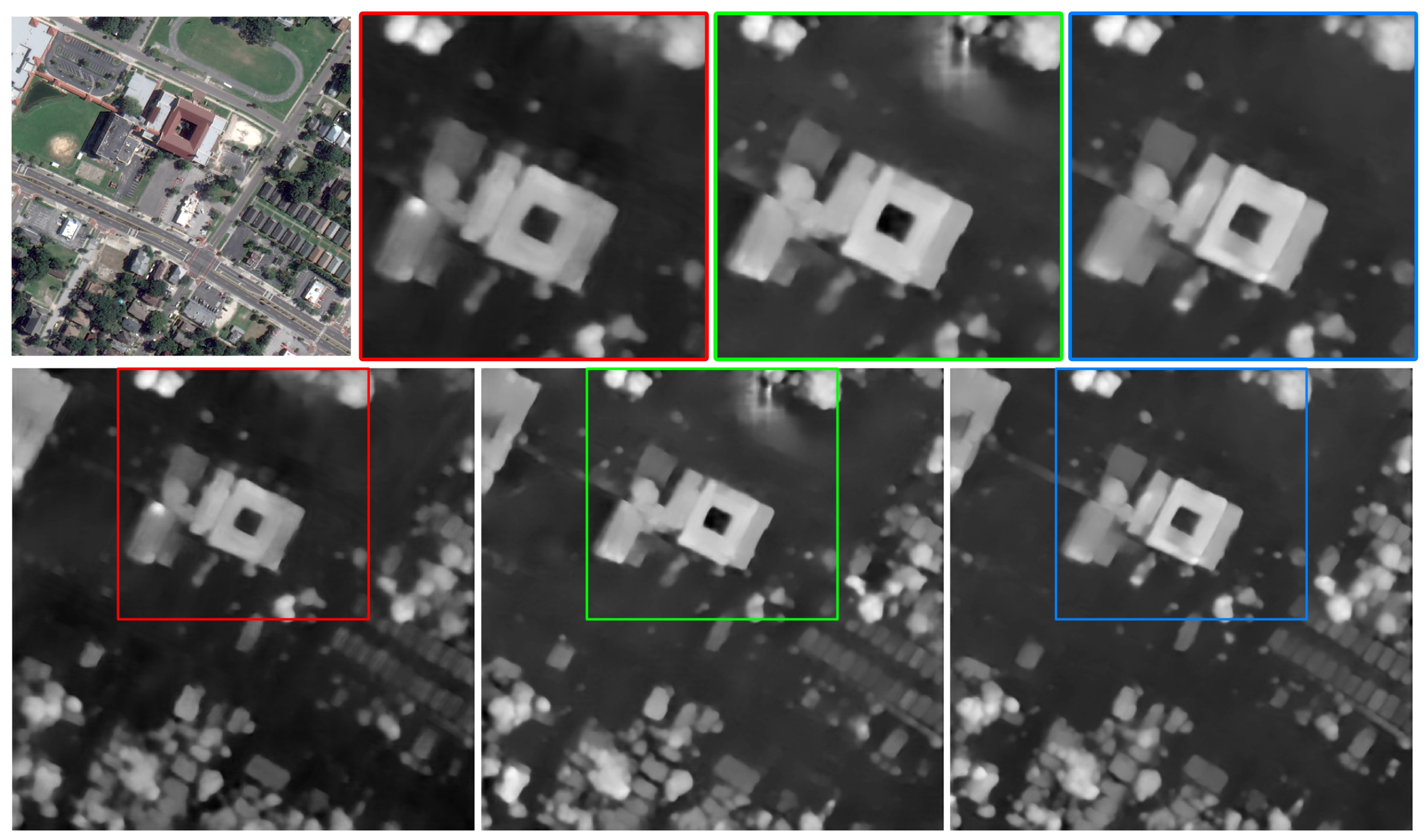
We also randomly select several image pairs from the JAX testing set and OMA set and list the disparity maps predicted by these models in Figure 4 (results of Bidir-EPNet are not listed since it hasn’t yet been open-source). It can be seen that our network outputs the disparity maps of the highest quality for these three images. For one thing, in regions with simple structures such as flat grounds and roads, DSM-Net predicts smooth disparities. For another, in regions containing objects with complex structures such as woods and small houses, DSM-Net can maintain their structures. DenseMapNet gives the worst prediction results. StereoNet performs well in the former category of regions but fails to recover details of the latter category, while PSMNet does the opposite. The reason is that both StereoNet and PSMNet only learn stereo matching at one scale, which cannot fit in well with changeful scenes in remote sensing images. By contrast, dual-scale learning works well in such challenges. Besides, mosaic occurs in the disparity maps output by PSMNet while doesn’t appear in that of StereoNet or DSM-Net (please zoom in to see details). That is because the latter two adopt refinement operations to guide the prediction of the decimated resolution to be up-sampled to higher resolution, while no refinement is used in PSMNet. Passingly, because we build cost volumes covering both non-negative and negative values for these networks, all of them are no longer limited to merely regress nonnegative disparities.
4.3.2. Result on Challenging Areas
To show how our method improves the disparity estimation on challenging areas that raise difficulties to the stereo matching of high-resolution remote sensing images, several stereo pairs containing typical scenes, such as texture-less regions, repetitive patterns, disparity discontinuities, and occlusions, are chosen to meticulously evaluate these models. Note that DenseMapNet performs far worse and Bidir-EPNet is not open-source, consequently, we mainly concentrate on the comparison between the other three.
Texture-less Regions. In these regions, intensities of pixels change feebly, making them difficult to distinguish, which can lead to ambiguous results. We list several examples of disparity estimation on texture-less regions in Figure 5. The lawn and highways are texture-less. DSM-Net performs best by outputting disparity maps with less ambiguity on all scenes. Empirically, the elevation of a piece of flat lawn is the same everywhere, DSM-Net predicts more consistent disparities than the others. The elevation of a sloping highway varies continuously, the disparity map output by DSM-Net is continuous, while discontinuity appears on that of the other two.
Repetitive Patterns. Image patches in these regions have extremely similar appearances, which can cause fuzzy matching. Several examples are depicted in Figure 6. Residences contained in the images exhibit similar textures and colors. In the disparity maps predicted by StereoNet and PSMNet, some residences are joined to the boundaries of their neighboring residences. While in the disparity maps output by our DSM-Net, most of the residences are discriminated, and the edges are better maintained, thus less confusion occurs.
DSM-Net performs better on the two types of challenges, we credit this to the dual-scale learning strategy, which can find stereo correspondences easily based on perceptions at different scales that capture both coarse-grained and fine-grained information. Meanwhile, important cues such as edges are taken full advantage of, and details are also better recovered. StereoNet learns matching based on only a low-resolution cost volume, thus some details and thin structures are lost. PSMNet forms a high-scale cost volume using features that have integrated multiscale context, however, the features are simply fused and indiscriminately processed. By contrast, DSM-Net exploits features of different scales but disposes of them severally, with a proper connection built between them.
Disparity Discontinuities and Occlusions. Disparity discontinuities can lead to the edge-fattening issue, and in occluded areas, there is no matching. Due to tall objects, such challenges are ubiquitous in remote sensing images. We demonstrate three examples of disparity estimation results on areas containing high buildings and other objects, as shown in Figure 7. There is an occluded shadow behind the building in the first image, StereoNet gives an obvious wrong disparity prediction that is inconsistent with the surrounding ground, while PSMNet and DSM-Net give consistent disparities, and disparity map output by DSM-Net is flatter. In the second image, the disparity maps output by PSMNet and DSM-Net show smooth transition around the building, especially in the facade, and the edges of buildings are more explicit in the disparity map output by DSM-Net. Predictions of the third image also indicate DSM-Net performs best. We argue that the 3D encoder-decoder module contributes to this improvement. In StereoNet, the cost is simply aggregated by five stacked 3D convolution layers. In DSM-Net, we aggregate the cost using the deeper module with subsampling and up-sampling operations. This design makes the module rectify wrong cost values with information captured from a larger view. Deeper layers make the cost aggregation module have a more powerful ability to approximate the matching for occlusions. PSMNet adopts a stacked multiple hourglass module for cost aggregation, which shares a similar idea to ours, and it can be seen that PSMNet also performs better than StereoNet.
Further, we quantitatively evaluate the results of different models on each individual of the aforementioned stereo pairs, as listed in Table 5. It can be noticed that our model achieves the best accuracy on all the stereo pairs. In summary, the proposed DSM-Net can more effectively deal with multiple challenges encountered by the disparity estimation of high-resolution remote sensing images.
5. Discussion
In this section, we conduct thorough ablation studies to verify our network design choices. Specifically, we train four variants of the proposed DSM-Net to explore how the dual-scale matching strategy, 3D encoder-decoder module, and refinement influence the stereo performance. Configurations and comparisons of the variants are listed in Table 6.
5.1. Single-Scale vs. Dual-Scale
We train two variants of DSM-Net that learn stereo matching only at one scale. DSM-Net-v1 only learns the low-scale matching while DSM-Net-v2 only learns the high-scale. Feature extractors in the variants only extract features of corresponding scales, and refinement is conducted on their estimated disparity maps. The dual-scale learning scheme outperforms its single-scale counterparts. That is because the low scale can capture a wide range but may lose details and thin structures around small objects, while the high scale does the opposite, thus learning at both scales is necessary. Estimated disparity maps in Figure 8 also confirm this. On the large texture-less playground, DSM-Net-v1 gives better disparity prediction than DSM-Net-v2, while on the building with complex structure, DSM-Net-v2 performs better. DSM-Net predicts continuous and smooth disparity on the playground and preserves the fine structure of the building. By the way, though the accuracy of DSM-Net-v1 drops a lot, it still outperforms the lightweight StereoNet [27] and runs extremely fast, which shows a potential to be deployed on resource-constrained devices.
5.2. Plain Module vs. Encoder-Decoder Module
To verify the effectiveness and efficiency of the 3D encoder-decoder module for cost aggregation, we train DSM-Net-v3 which uses a plain module consisting of nine simply stacked standard 3D convolutions (shown in Figure 9) and has a close number of parameters to the encoder-decoder module.
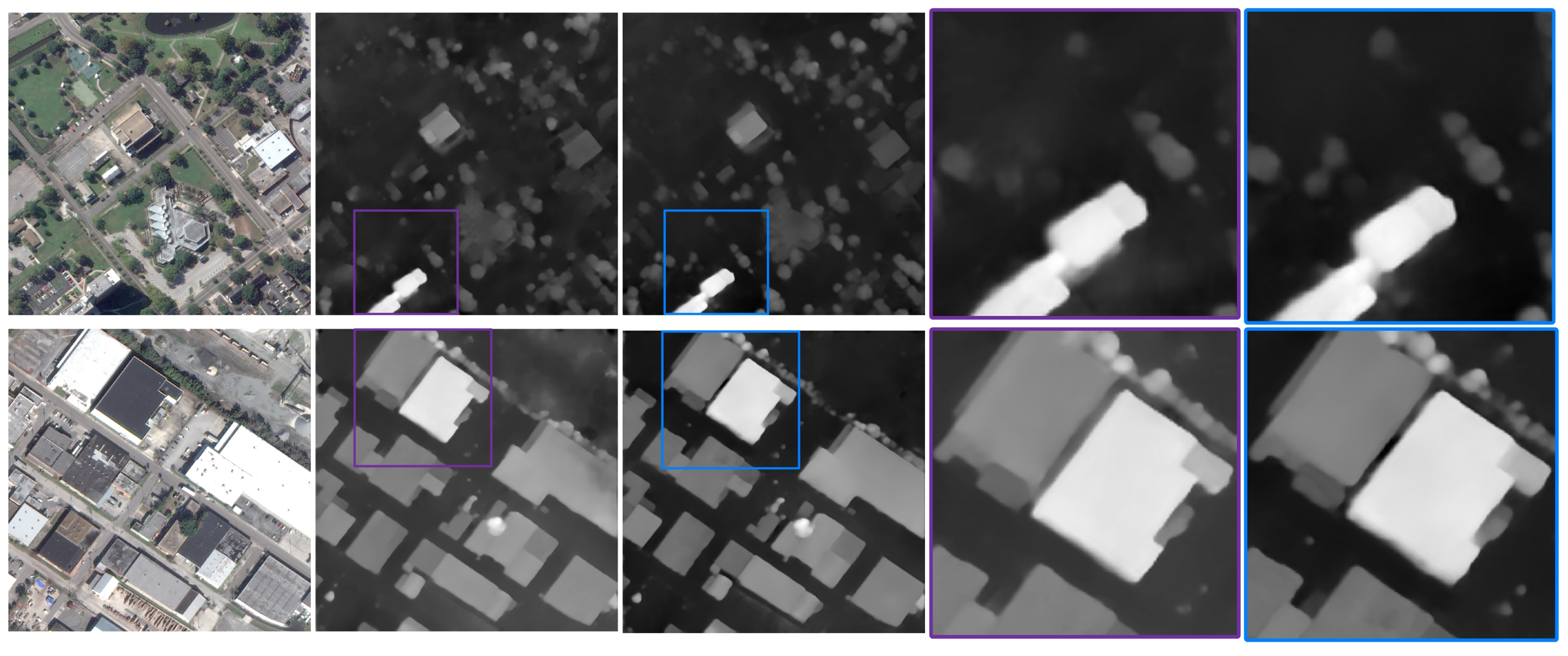
It can be observed from Table 6 that if the 3D encoder-decoder is replaced with a plain module, the stereo performance will degrade in terms of both accuracy and efficiency. Figure 10 indicates that the 3D encoder-decoder can better approximate matching for occluded areas and address the edge-fattening issue. DSM-Net predicts smooth disparities in the occluded shadow and unambiguous disparities around high buildings. That is because the encoder-decoder design learns cost aggregation and geometric context more efficiently. DSM-Net takes almost a third as long as DSM-Net-v3 to process a stereo pair, though they have a close number of parameters. This is due to the factorized 3D convolution, which is much more computationally economical. With factorized 3D convolutions, we can build deeper and faster networks using a similar number of parameters.
5.3. Without Refinement vs. With Refinement
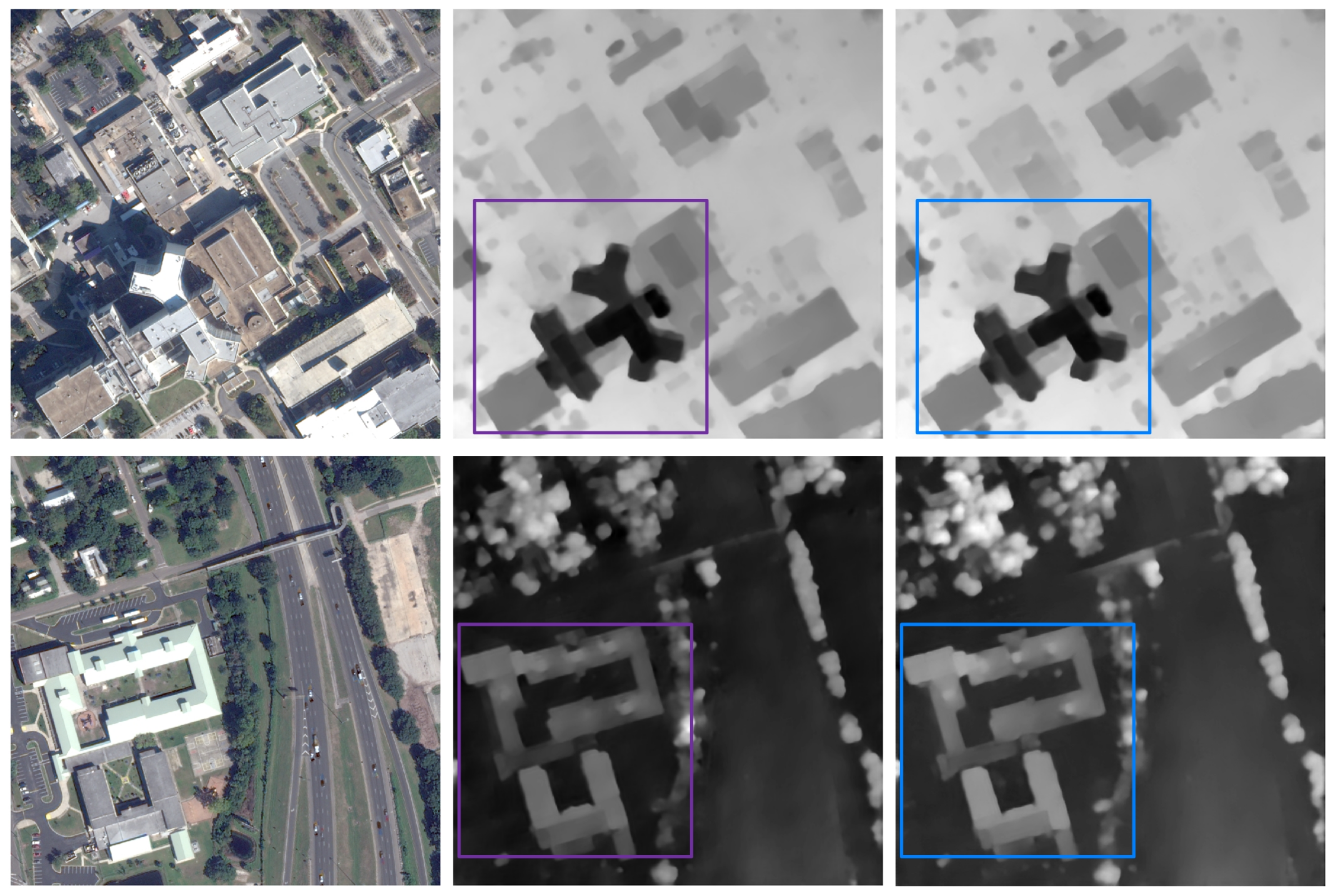
The refinement operation can improve the quality of an estimated disparity map. We train DSM-Net-v4 that removes the refinement module to clarify the importance. Table 6 depicts the accuracy comparison. The refinement operation further improves the accuracy at the expense of negligible time increases. More significantly, due to the high-frequency information contained in the shallow features being introduced, the refinement module can alleviate mosaics in the up-sampled full-resolution disparity maps, as well as bring in more fine details, as shown in Figure 11.
6. Conclusions
In this paper, we propose a novel end-to-end CNN architecture named dual-scale matching network (DSM-Net) for disparity estimation of high-resolution remote sensing images. Aiming at the difficulties encountered by stereo matching of remote sensing images, our network provides corresponding solutions. By learning dual-scale matching, constructing cost volumes covering both negative and nonnegative disparities, aggregating cost with a factorized 3D encoder-decoder, and employing a refinement operation, our network shows a strong ability to estimate disparities, as well as a satisfactory generalization ability. Extensive experimental results and comparisons with state-of-the-art methods demonstrate that our approach can handle multi-type challenges more effectively and efficiently. In particular, stereo matching in problematic regions is notably ameliorated. Moreover, thorough ablation studies verify the effectiveness of our network design choices. By training variants of the proposed network and comparing their results, we demonstrate how each of the design choices improves the model.
In the future, we are going to further improve the performance, and explore how to make the network be trained in a semi-supervised or unsupervised way to further expand its versatility since it is trained in a fully supervised manner and requires large numbers of ground-truth labels at the present stage.
Author Contributions
Conceptualization, S.H.; methodology, S.H.; validation, R.Z.; writing—original draft preparation, S.H.; writing—review and editing, R.Z.; visualization, S.L.; supervision, S.J. and W.J. All authors have read and agreed to the published version of the manuscript.
Funding
This research was funded by the High-Resolution Remote Sensing Application Demonstration System for Urban Fine Management (grant number 06-Y30F04-9001-20/22) and the National Natural Science Foundation of China (grant number 42001413).
Institutional Review Board Statement
Not applicable.
Informed Consent Statement
Not applicable.
Data Availability Statement
The US3D track-2 dataset can be found at https://ieee-dataport.org/open-access/data-fusion-contest-2019-dfc2019 (access date: 26 November 2018). Codes and trained models are available at https://github.com/Sheng029/StereoMatchingRemoteSensing (access date: 10 October 2021).
Acknowledgments
The authors would like to thank IARPA and the Johns Hopkins University Applied Physics Laboratory for providing the wonderful dataset, and the developers in the TensorFlow community for their open-source deep learning projects. The authors would also like to express their gratitude to the editors and reviewers for their constructive and helpful comments.
Conflicts of Interest
The authors declare no conflict of interest.
References
- Kang, J.H.; Chen, L.; Deng, F.; Heipke, C. Context pyramidal network for stereo matching regularized by disparity gradients. ISPRS-J. Photogramm. Remote Sens. 2019, 157, 201–215. [Google Scholar] [CrossRef]
- Hirschmuller, H. Accurate and efficient stereo processing by semi-global matching and mutual information. In Proceedings of the IEEE Conference on Computer Vision and Pattern Recognition, San Diego, CA, USA, 20–25 June 2005; pp. 807–814. [Google Scholar]
- Zhang, L.; Seitz, S.M. Estimating optimal parameters for MRF stereo from a single image pair. IEEE Trans. Pattern Anal. Mach. Intell. 2007, 29, 331–342. [Google Scholar] [CrossRef] [PubMed] [Green Version]
- Hirschmueller, H.; Scharstein, D. Evaluation of cost functions for stereo matching. In Proceedings of the IEEE Conference on Computer Vision and Pattern Recognition, Minneapolis, MO, USA, 17–22 June 2007. [Google Scholar]
- Rhemann, C.; Hosni, A.; Bleyer, M.; Rother, C.; Gelautz, M. Fast Cost-Volume Filtering for Visual Correspondence and Beyond. In Proceedings of the IEEE Conference on Computer Vision and Pattern Recognition, Colorado Springs, CO, USA, 20–25 June 2011. [Google Scholar]
- Scharstein, D.; Szeliski, R. A taxonomy and evaluation of dense two-frame stereo correspondence algorithms. Int. J. Comput. Vis. 2002, 47, 7–42. [Google Scholar] [CrossRef]
- Krizhevsky, A.; Sutskever, I.; Hinton, G.E. ImageNet Classification with Deep Convolutional Neural Networks. Commun. ACM. 2017, 60, 84–90. [Google Scholar] [CrossRef]
- Shelhamer, E.; Long, J.; Darrell, T. Fully Convolutional Networks for Semantic Segmentation. IEEE Trans. Pattern Anal. Mach. Intell. 2017, 39, 640–651. [Google Scholar] [CrossRef] [PubMed]
- Girshick, R.; Donahue, J.; Darrell, T.; Malik, J. Rich feature hierarchies for accurate object detection and semantic segmentation. In Proceedings of the IEEE Conference on Computer Vision and Pattern Recognition, Columbus, GA, USA, 23–28 June 2014; pp. 580–587. [Google Scholar]
- Eigen, D.; Puhrsch, C.; Fergus, R. Depth Map Prediction from a Single Image using a Multi-Scale Deep Network. In Proceedings of the Conference on Neural Information Processing Systems, Montreal, WI, USA, 8–13 December 2014. [Google Scholar]
- Zbontar, J.; LeCun, Y. Stereo Matching by Training a Convolutional Neural Network to Compare Image Patches. J. Mach. Learn. Res. 2016, 17, 65. [Google Scholar]
- Luo, W.J.; Schwing, A.G.; Urtasun, R. Efficient Deep Learning for Stereo Matching. In Proceedings of the IEEE Conference on Computer Vision and Pattern Recognition, Seattle, WA, USA, 27–30 June 2016; pp. 5695–5703. [Google Scholar]
- Park, H.; Lee, K.M. Look Wider to Match Image Patches With Convolutional Neural Networks. IEEE Signal Process. Lett. 2017, 24, 1788–1792. [Google Scholar] [CrossRef] [Green Version]
- Seki, A.; Pollefeys, M. Patch based confidence prediction for dense disparity map. In Proceedings of the British Machine Vision Conference, York, UK, 19–22 September 2016. [Google Scholar]
- Seki, A.; Pollefeys, M. SGM-Nets: Semi-global matching with neural networks. In Proceedings of the IEEE Conference on Computer Vision and Pattern Recognition, Honolulu, HI, USA, 21–26 July 2017; pp. 6640–6649. [Google Scholar]
- Shaked, A.; Wolf, L. Improved Stereo Matching with Constant Highway Networks and Reflective Confidence Learning. In Proceedings of the IEEE Conference on Computer Vision and Pattern Recognition, Honolulu, HI, USA, 21–27 July 2017; pp. 6901–6910. [Google Scholar]
- Ye, X.Q.; L, J.M.; Wang, H.; Huang, H.X.; Zhang, X.L. Efficient Stereo Matching Leveraging Deep Local and Context Information. IEEE Access. 2017, 5, 18745–18755. [Google Scholar] [CrossRef]
- Poggi, M.; Tosi, F.; Batsos, K.; Mordohai, P.; Mattoccia, S. On the Synergies between Machine Learning and Binocular Stereo for Depth Estimation from Images: A Survey. IEEE Trans. Pattern Anal. Mach. Intell. 2021. [Google Scholar] [CrossRef] [PubMed]
- Liang, Z.F.; Feng, Y.L.; Guo, Y.L.; Liu, H.Z.; Chen, W.; Qiao, L.B.; Zhou, L.; Zhang, J.F. Learning for Disparity Estimation through Feature Constancy. In Proceedings of the IEEE Conference on Computer Vision and Pattern Recognition, Salt Lake City, UT, USA, 18–23 June 2018; pp. 2811–2820. [Google Scholar]
- Mayer, N.; Ilg, E.; Hausser, P.; Fischer, P.; Cremers, D.; Dosovitskiy, A.; Brox, T. A Large Dataset to Train Convolutional Networks for Disparity, Optical Flow, and Scene Flow Estimation. In Proceedings of the IEEE Conference on Computer Vision and Pattern Recognition, Seattle, WA, USA, 27–30 June 2016; pp. 4040–4048. [Google Scholar]
- Dosovitskiy, A.; Fischer, P.; Ilg, E.; Haeusser, P.; Hazirbas, C.; Golkov, V.; van der Smagt, P.; Cremers, D.; Brox, T. FlowNet: Learning Optical Flow with Convolutional Networks. In Proceedings of the IEEE International Conference on Computer Vision, Santiago, Chile, 11–18 December 2015; pp. 2758–2766. [Google Scholar]
- Kendall, A.; Martirosyan, H.; Dasgupta, S.; Henry, P.; Kennedy, R.; Bachrach, A.; Bry, A. End-to-End Learning of Geometry and Context for Deep Stereo Regression. In Proceedings of the IEEE International Conference on Computer Vision, Venice, Italy, 22–29 October 2017; pp. 66–75. [Google Scholar]
- Pang, J.H.; Sun, W.X.; Ren, J.S.J.; Yang, C.X.; Yan, Q. Cascade Residual Learning: A Two-stage Convolutional Neural Network for Stereo Matching. In Proceedings of the IEEE International Conference on Computer Vision, Venice, Italy, 22–29 October 2017; pp. 878–886. [Google Scholar]
- Tonioni, A.; Tosi, F.; Poggi, M.; Mattoccia, S.; di Stefano, L. Real-time self-adaptive deep stereo. In Proceedings of the IEEE Conference on Computer Vision and Pattern Recognition, Long Beach, CA, USA, 16–20 June 2019; pp. 195–204. [Google Scholar]
- Xu, H.F.; Zhang, J.Y. AANet: Adaptive Aggregation Network for Efficient Stereo Matching. In Proceedings of the IEEE Conference on Computer Vision and Pattern Recognition, Electr Network, 14–19 June 2020; pp. 1956–1965. [Google Scholar]
- Chang, J.R.; Chen, Y.S. Pyramid Stereo Matching Network. In Proceedings of the IEEE Conference on Computer Vision and Pattern Recognition, Salt Lake City, UT, USA, 18–23 June 2018; pp. 5410–5418. [Google Scholar]
- Khamis, S.; Fanello, S.; Rhemann, C.; Kowdle, A.; Valentin, J.; Izadi, S. StereoNet: Guided Hierarchical Refinement for Real-Time Edge-Aware Depth Prediction. In Proceedings of the European Conference on Computer Vision, Munich, Germany, 8–14 September 2018; pp. 596–613. [Google Scholar]
- Yu, L.D.; Wang, Y.C.; Wu, Y.W.; Jia, Y.D. Deep Stereo Matching with Explicit Cost Aggregation Sub-Architecture. In Proceedings of the Innovative Applications of Artificial Intelligence Conference, New Orleans, LA, USA, 2–7 February 2018; pp. 7517–7524. [Google Scholar]
- Chabra, R.; Straub, J.; Sweeney, C.; Newcombe, R.; Fuchs, H. StereoDRNet: Dilated Residual StereoNet. In Proceedings of the IEEE Conference on Computer Vision and Pattern Recognition, Long Beach, CA, USA, 16–20 June 2019; pp. 11778–11787. [Google Scholar]
- Xing, J.B.; Qi, Z.; Dong, J.Y.; Cai, J.X.; Liu, H. MABNet: A Lightweight Stereo Network Based on Multibranch Adjustable Bottleneck Module. In Proceedings of the European Conference on Computer Vision, Glasgow, UK, 23–28 August 2020; pp. 340–356. [Google Scholar]
- Geiger, A.; Lenz, P.; Urtasun, R. Are we ready for autonomous driving? The KITTI vision benchmark suite. In Proceedings of the IEEE Conference on Computer Vision and Pattern Recognition, Providence, RI, USA, 16–21 June 2012; pp. 2018–2025. [Google Scholar]
- Menze, M.; Geiger, A. Object Scene Flow for Autonomous Vehicles. In Proceedings of the IEEE Conference on Computer Vision and Pattern Recognition, Boston, MA, USA, 7–12 June 2015; pp. 3061–3070. [Google Scholar]
- Scharstein, D.; Hirschmüller, H.; Kitajima, Y.; Krathwohl, G.; Nešić, N.; Wang, X.; Westling, P. High-Resolution Stereo Datasets with Subpixel-Accurate Ground Truth. In Proceedings of the German Conference on Pattern Recognition, Münster, Germany, 2–5 September 2014; pp. 31–42. [Google Scholar]
- Mayer, N.; Ilg, E.; Fischer, P.; Hazirbas, C.; Cremers, D.; Dosovitskiy, A.; Brox, T. What Makes Good Synthetic Training Data for Learning Disparity and Optical Flow Estimation? Int. J. Comput. Vis. 2018, 126, 942–960. [Google Scholar] [CrossRef] [Green Version]
- Ji, S.P.; Liu, J.; Lu, M. CNN-Based Dense Image Matching for Aerial Remote Sensing Images. Photogramm. Eng. Remote Sens. 2019, 85, 415–424. [Google Scholar] [CrossRef]
- Tao, R.S.; Xiang, Y.M.; You, H.J. An Edge-Sense Bidirectional Pyramid Network for Stereo Matching of VHR Remote Sensing Images. Remote Sens. 2020, 12, 4025. [Google Scholar] [CrossRef]
- Tran, D.; Wang, H.; Torresani, L.; Ray, J.; LeCun, Y.; Paluri, M. A Closer Look at Spatiotemporal Convolutions for Action Recognition. In Proceedings of the IEEE Conference on Computer Vision and Pattern Recognition, Salt Lake City, UT, USA, 18–23 June 2018; pp. 6450–6459. [Google Scholar]
- He, K.M.; Zhang, X.Y.; Ren, S.Q.; Sun, J. Spatial Pyramid Pooling in Deep Convolutional Networks for Visual Recognition. IEEE Trans. Pattern Anal. Mach. Intell. 2015, 37, 1904–1916. [Google Scholar] [CrossRef] [PubMed] [Green Version]
- Chopra, S.; Hadsell, R.; LeCun, Y. Learning a similarity metric discriminatively, with application to face verification. In Proceedings of the IEEE Conference on Computer Vision and Pattern Recognition, San Diego, CA, USA, 20–25 June 2005; pp. 539–546. [Google Scholar]
- He, K.M.; Zhang, X.Y.; Ren, S.Q.; Sun, J. Deep Residual Learning for Image Recognition. In Proceedings of the IEEE Conference on Computer Vision and Pattern Recognition, Seattle, WA, USA, 27–30 June 2016; pp. 770–778. [Google Scholar]
- Ioffe, S.; Szegedy, C. Batch Normalization: Accelerating Deep Network Training by Reducing Internal Covariate Shift. In Proceedings of the International Conference on Machine Learning, Lille, France, 7–9 July 2015; pp. 448–456. [Google Scholar]
- Zeiler, M.D.; Taylor, G.W.; Fergus, R. Adaptive Deconvolutional Networks for Mid and High Level Feature Learning. In Proceedings of the IEEE International Conference on Computer Vision, Barcelona, Spain, 6–13 November 2011; pp. 2018–2025. [Google Scholar]
- Fisher, Y.; Vladlen, K. Multi-Scale Context Aggregation by Dilated Convolutions. arXiv 2015, arXiv:1511.07122. Available online: https://arxiv.org/abs/1511.07122 (accessed on 23 November 2015).
- Girshick, R. Fast R-CNN. In Proceedings of the IEEE International Conference on Computer Vision, Santiago, Chile, 11–18 December 2015; pp. 1440–1448. [Google Scholar]
- Bosch, M.; Foster, K.; Christie, G.; Wang, S.; Hager, G.D.; Brown, M. Semantic Stereo for Incidental Satellite Images. In Proceedings of the IEEE Winter Conference on Applications of Computer Vision, Waikoloa Village, HI, USA, 7–11 January 2019; pp. 1524–1532. [Google Scholar]
- Le Saux, B.; Yokoya, N.; Hansch, R.; Brown, M.; Hager, G. 2019 Data Fusion Contest [Technical Committees]. IEEE Geosci. Remote Sens. Mag. 2019, 7, 103–105. [Google Scholar] [CrossRef]
- Martin, A.; Agarwal, A.; Barham, P.; Brevdo, E.; Chen, Z.; Citro, C.; Corrado, G.S.; Davis, A.; Dean, J.; Devin, M.; et al. TensorFlow: Large-Scale Machine Learning on Heterogeneous Distributed Systems. arXiv 2016, arXiv:1603.04467. Available online: https://arxiv.org/abs/1603.04467 (accessed on 14 March 2016).
- Atienza, R. Fast Disparity Estimation using Dense Networks. In Proceedings of the IEEE International Conference on Robotics and Automation, Brisbane, Australia, 21–25 May 2018; pp. 3207–3212. [Google Scholar]
Figure 1.
Overview of DSM-Net, which consists of five components, including feature extraction, cost volume creation, cost aggregation, disparity calculation, and disparity refinement.
Figure 1.
Overview of DSM-Net, which consists of five components, including feature extraction, cost volume creation, cost aggregation, disparity calculation, and disparity refinement.

Figure 2.
The operation for the cost volume creation. The right feature shifts from to , making the resulting cost volume covering the range [, ).
Figure 2.
The operation for the cost volume creation. The right feature shifts from to , making the resulting cost volume covering the range [, ).

Figure 3.
The architecture of the refinement module. Dilated convolutions [43] are used within the module, “dilation” denotes the dilation rate, “s” denotes the convolution stride. Each convolution layer is followed by a batch normalization layer and a leaky ReLU activation layer (), except the 1*1*3 and 3*3*1 layer.

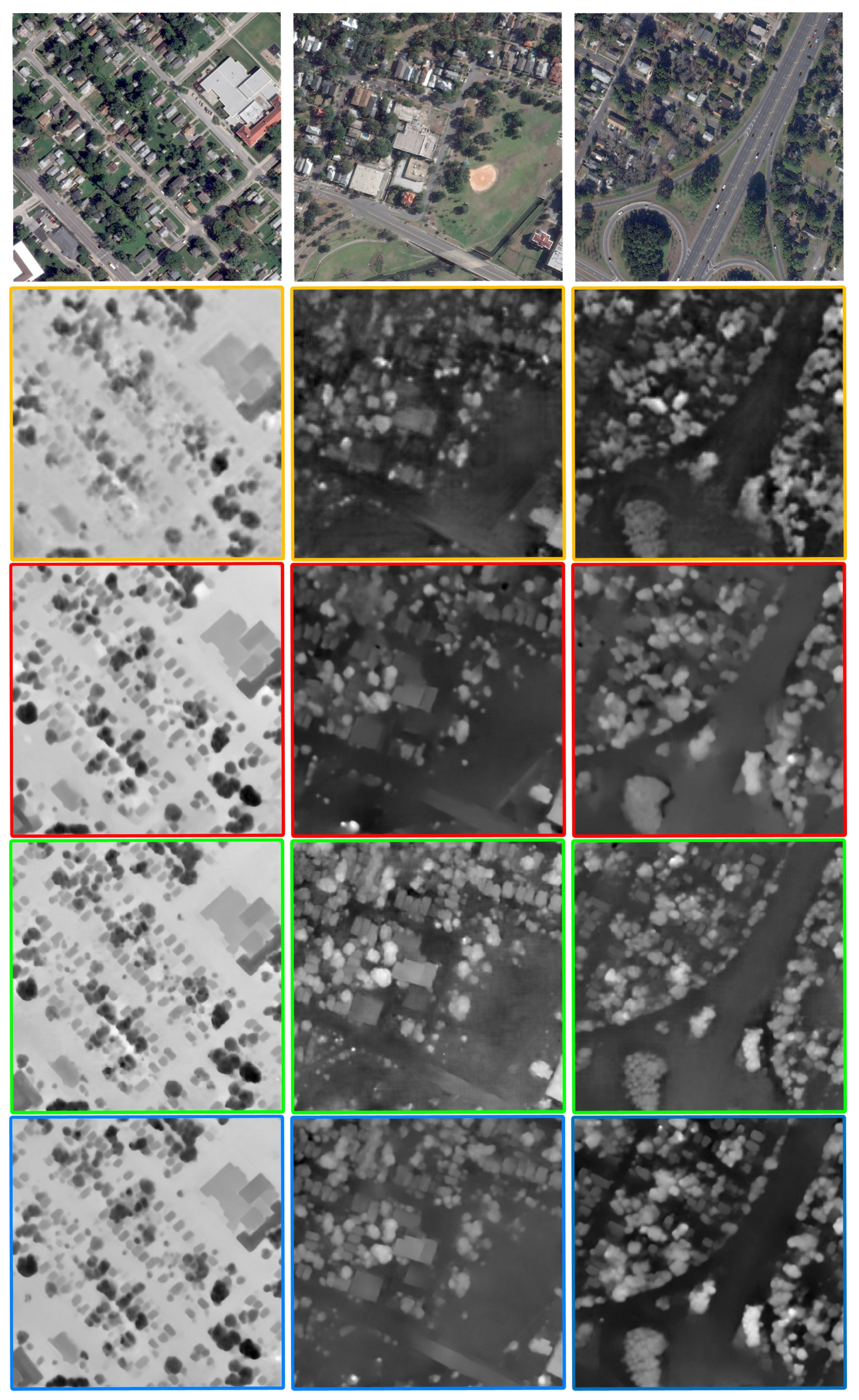
Figure 4.
Disparity maps output by different networks. The image in the first column is from the OMA set, and the others are from the JAX testing set. Predictions of DenseMapNet, StereoNet, PSMNet, and DSM-Net are respectively labeled with yellow, red, green, and blue.
Figure 4.
Disparity maps output by different networks. The image in the first column is from the OMA set, and the others are from the JAX testing set. Predictions of DenseMapNet, StereoNet, PSMNet, and DSM-Net are respectively labeled with yellow, red, green, and blue.

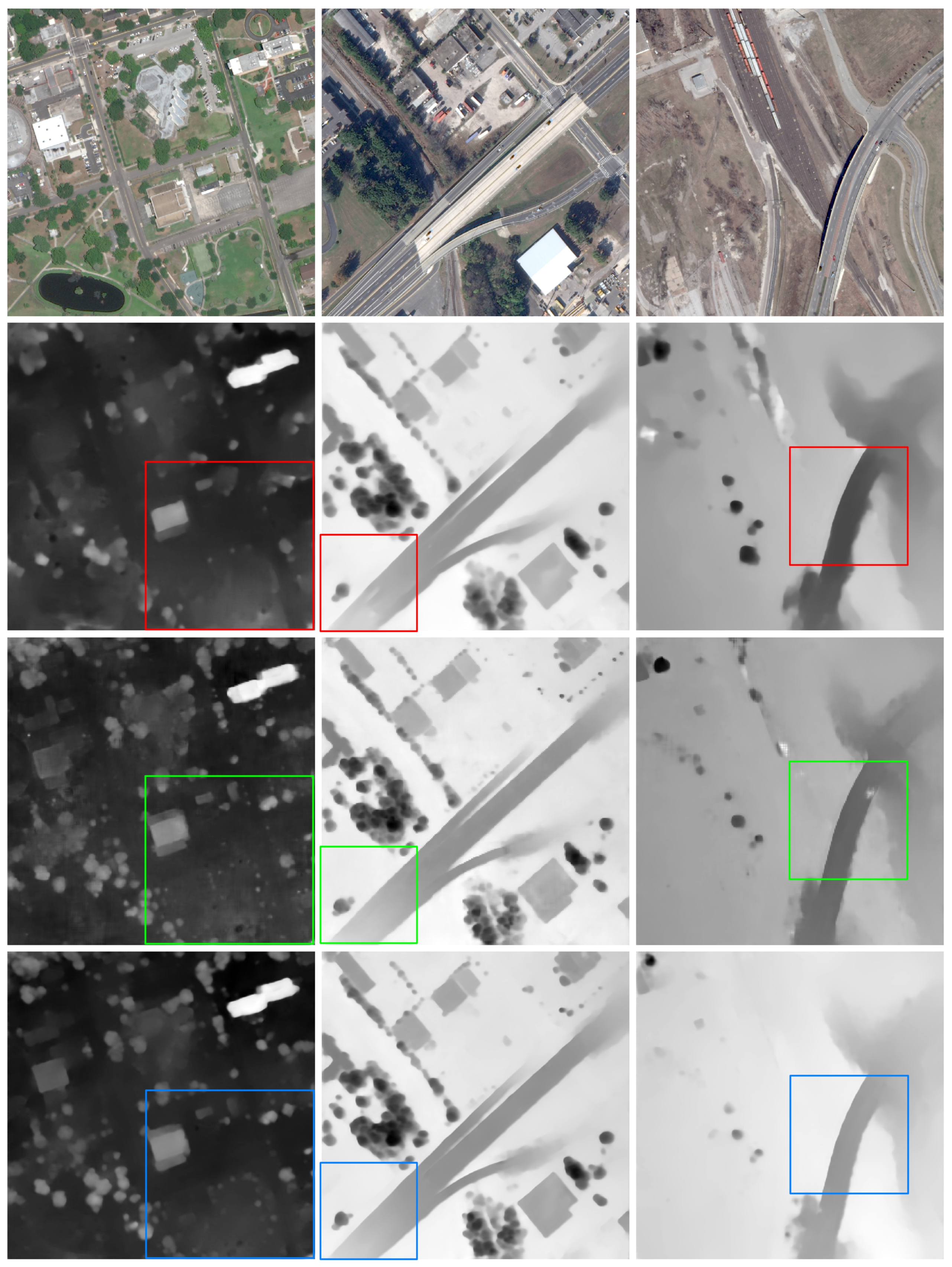
Figure 5.
Disparity estimation results of different models on texture-less regions. Predictions of StereoNet, PSMNet, and DSM-Net are respectively labeled with red, green, and blue (subsequent figures in this section are also labeled in this way). Tile numbers are JAX-122-019-005, JAX-079-006-007, and OMA-211-026-006, from left to right.

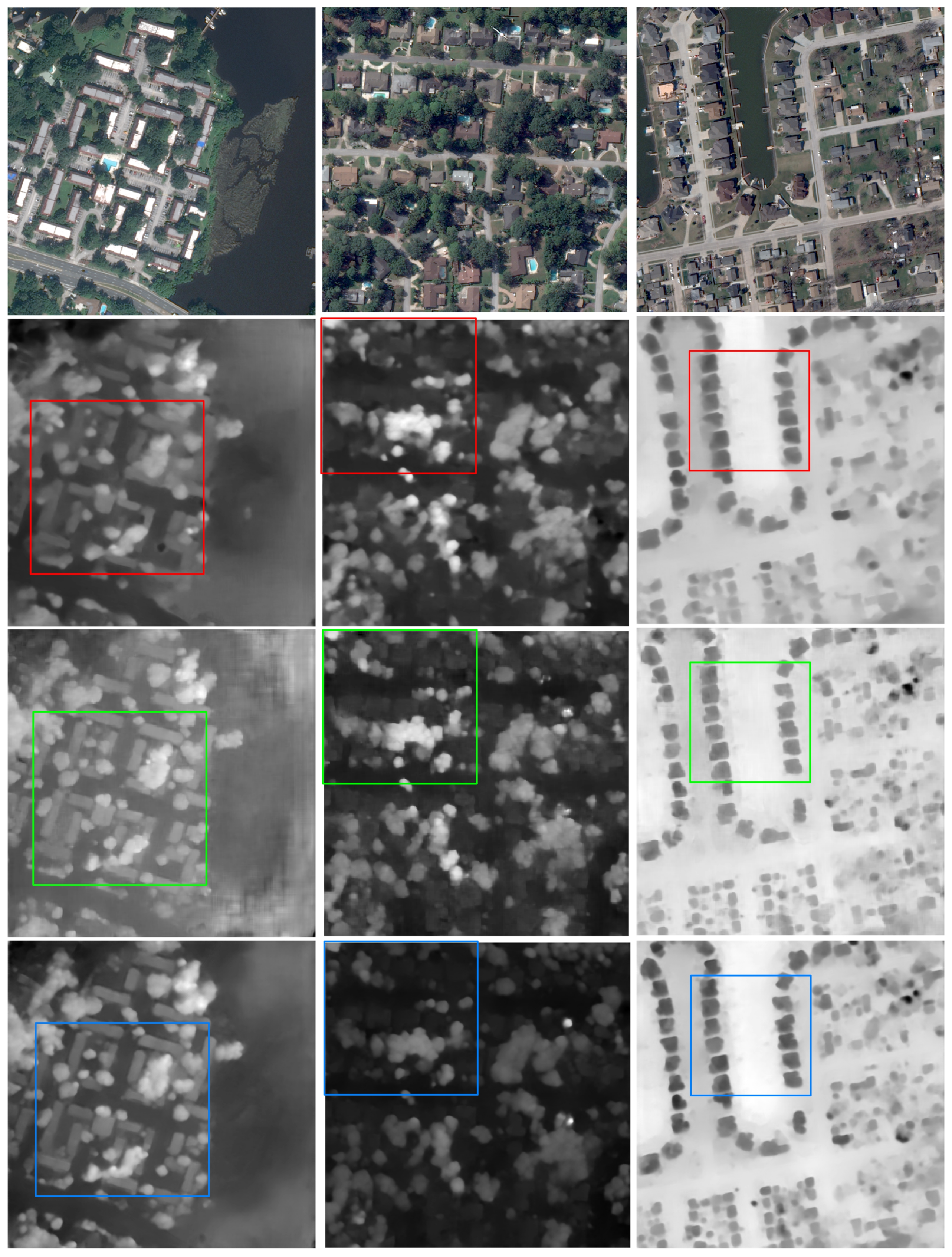
Figure 6.
Disparity estimation results of different models on repetitive patterns. Tile numbers are JAX-280-021-020, JAX-559-022-002, and OMA-132-027-023, from left to right.
Figure 6.
Disparity estimation results of different models on repetitive patterns. Tile numbers are JAX-280-021-020, JAX-559-022-002, and OMA-132-027-023, from left to right.

Figure 7.
Disparity estimation results of different models on disparity discontinuities and occluded areas. Tile numbers are JAX-072-011-022, JAX-264-014-007, and OMA-212-007-005, from left to right.
Figure 7.
Disparity estimation results of different models on disparity discontinuities and occluded areas. Tile numbers are JAX-072-011-022, JAX-264-014-007, and OMA-212-007-005, from left to right.

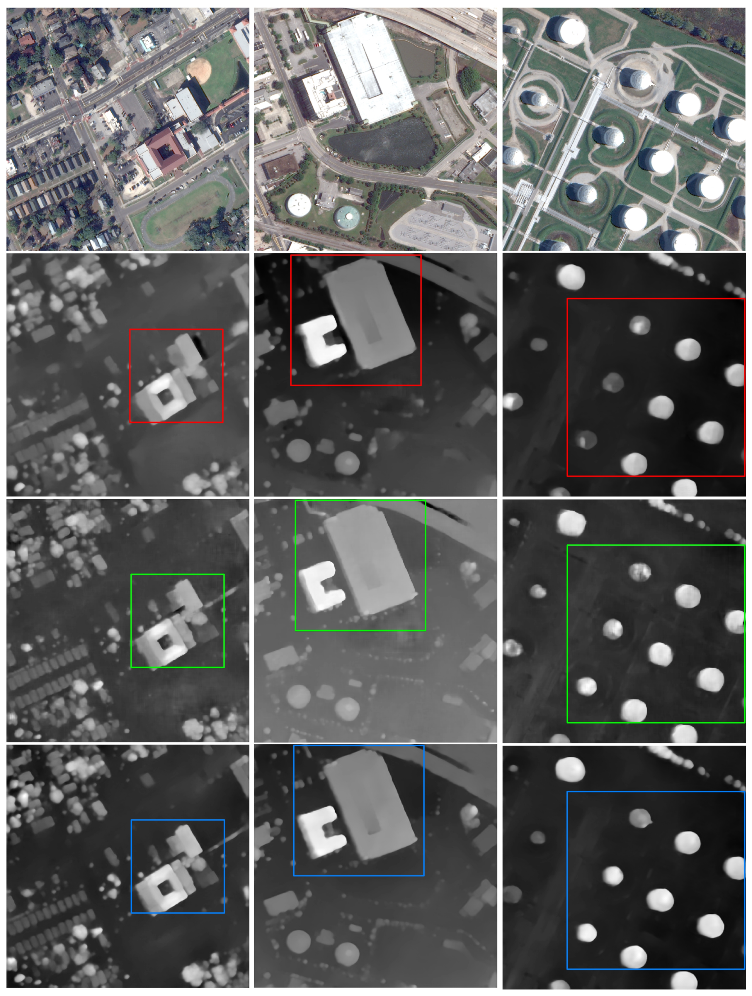
Figure 8.
Disparity maps output by networks with single-scale and dual-scale learning schemes (tile number: JAX-072-001-006). The outputs of DSM-Net-v1, DSM-Net-v2, and DSM-Net are labeled with red, green, and blue, respectively.
Figure 8.
Disparity maps output by networks with single-scale and dual-scale learning schemes (tile number: JAX-072-001-006). The outputs of DSM-Net-v1, DSM-Net-v2, and DSM-Net are labeled with red, green, and blue, respectively.

Figure 9.
The plain module for cost aggregation in DSM-Net-v3. In this variant, the 4D volume output by the eighth convolution layer at the low scale is up-sampled and added to the initial cost volume at the high scale. Each convolution layer is followed by a batch normalization layer and a leaky ReLU activation layer (), except for the last two layers.

Figure 10.
Disparity maps output by networks with different cost aggregation modules (tile number: JAX-122-022-002, JAX-156-009-003). The outputs of DSM-Net-v3 and DSM-Net are respectively labeled with purple and blue.
Figure 10.
Disparity maps output by networks with different cost aggregation modules (tile number: JAX-122-022-002, JAX-156-009-003). The outputs of DSM-Net-v3 and DSM-Net are respectively labeled with purple and blue.

Figure 11.
Disparity maps output by networks without and with refinement operations (tile number: JAX-068-006-012, JAX-113-004-011). The outputs of DSM-Net-v4 and DSM-Net are respectively labeled with purple and blue.
Figure 11.
Disparity maps output by networks without and with refinement operations (tile number: JAX-068-006-012, JAX-113-004-011). The outputs of DSM-Net-v4 and DSM-Net are respectively labeled with purple and blue.


Table 1.
The architecture of the shared 2D CNN. Construction of residual blocks is designated in brackets with the number of stacked blocks, “s” denotes the stride of convolution. Each convolution layer is followed by a batch normalization [41] layer and a ReLU activation layer, except conv1_3 and conv2_3.
| Name | Setting | Output | |||
|---|---|---|---|---|---|
| Input | H × W × 3 | ||||
| conv0_1 | 5 × 5 × 32, s = 2 | ×× 32 | |||
| conv0_2 | 5 × 5 × 32, s = 2 | ×× 32 | |||
| conv0_3 | ×× 32 | ||||
| Low scale | High scale | ||||
| conv2_1 | 3 × 3 × 32, s = 2 | ×× 32 | conv1_1 | 3 × 3 × 32 | ×× 32 |
| conv2_2 | ×× 32 | conv1_2 | ×× 32 | ||
| conv2_3 | 3×3×16 | ×× 16 | conv1_3 | 3×3×16 | ×× 16 |
Table 2.
The architecture of the 3D encoder-decoder module for cost aggregation, each convolution layer is followed by a batch normalization layer and a leaky ReLU activation layer (), except conv14 and conv15. Factorized 3D convolutions are designated in brackets, “s” denotes the stride of convolution, and “” denotes the transpose convolution [42]. Note that we use two independent modules with the same structure to separately aggregate the cost volumes, the output of conv14 at the low scale is up-sampled and added to the initial high-scale cost volume before the high-scale aggregation. For an input image of size and evaluating a range of D candidate disparities, the cost volume is of size for k subsampling operations.
| Name | Setting | Low Scale | High Scale |
|---|---|---|---|
| Cost volume | |||
| conv1 | |||
| conv2 | |||
| conv3 | |||
| conv4 | |||
| conv5 | |||
| conv6 | |||
| conv7 | |||
| conv8 | |||
| conv9 | |||
| conv10 | |||
| conv11 | |||
| conv12 | |||
| conv13 | |||
| conv14 | |||
| conv15 |
Table 3.
The usage of the dataset in our experiments. “JAX” represents Jacksonville and “OMA” represents Omaha (the same below).
Table 3.
The usage of the dataset in our experiments. “JAX” represents Jacksonville and “OMA” represents Omaha (the same below).
| Stereo Pair | Mode | Training/Validation/Testing | Usage |
|---|---|---|---|
| JAX | RGB | 1500/139/500 | Training, validation, and testing |
| OMA | RGB | -/-/2153 | Testing |
Table 4.
Quantitative results of different methods on the JAX testing set and the whole OMA set. The best results are bold.
Table 4.
Quantitative results of different methods on the JAX testing set and the whole OMA set. The best results are bold.
| Model | JAX | OMA | Time (ms) | ||
|---|---|---|---|---|---|
| EPE (Pixel) | D1 (%) | EPE (Pixel) | D1 (%) | ||
| DenseMapNet | 1.7405 | 14.19 | 1.8581 | 14.88 | 81 |
| StereoNet | 1.4356 | 10.00 | 1.5804 | 10.37 | 187 |
| PSMNet | 1.2968 | 8.06 | 1.4937 | 8.74 | 436 |
| Bidir-EPNet | 1.2764 | 8.03 | 1.4899 | 8.96 | - |
| DSM-Net | 1.2776 | 7.94 | 1.4757 | 8.73 | 168 |
Table 5.
Quantitative results of different models on individuals of specific stereo pairs from the JAX testing set and OMA set. The best results are bold.
Table 5.
Quantitative results of different models on individuals of specific stereo pairs from the JAX testing set and OMA set. The best results are bold.
| Tile | EPE (Pixel) | D1 (%) | ||||||
|---|---|---|---|---|---|---|---|---|
| DenseMapNet | StereoNet | PSMNet | DSM-Net | DenseMapNet | StereoNet | PSMNet | DSM-Net | |
| JAX-122-019-005 | 1.5085 | 1.4992 | 1.4815 | 1.2292 | 7.84 | 8.17 | 4.52 | 3.65 |
| JAX-079-006-007 | 1.6281 | 1.3743 | 1.2158 | 1.2082 | 12.42 | 9.71 | 8.46 | 8.16 |
| OMA-211-026-006 | 1.9534 | 1.5783 | 1.5739 | 1.4830 | 15.92 | 10.67 | 9.23 | 9.05 |
| JAX-280-021-020 | 1.3427 | 1.1412 | 1.0413 | 0.9772 | 10.42 | 6.75 | 6.26 | 5.43 |
| JAX-559-022-002 | 1.5756 | 1.5323 | 1.3536 | 1.2977 | 15.03 | 13.56 | 10.55 | 10.14 |
| OMA-132-027-023 | 1.5421 | 1.4018 | 1.3657 | 1.3054 | 11.84 | 9.61 | 9.21 | 8.45 |
| JAX-072-011-022 | 1.6813 | 1.3914 | 1.1675 | 1.0718 | 17.42 | 8.22 | 6.71 | 5.27 |
| JAX-264-014-007 | 1.6105 | 1.3083 | 1.0688 | 1.0528 | 15.54 | 6.67 | 4.65 | 3.81 |
| OMA-212-007-005 | 1.6740 | 1.3359 | 1.2587 | 1.1720 | 11.51 | 7.79 | 6.90 | 5.26 |
Table 6.
Configurations and comparisons of the variants. The best results are bold, the checkmark indicates that the network has this configuration.
Table 6.
Configurations and comparisons of the variants. The best results are bold, the checkmark indicates that the network has this configuration.
| Model | Scale | Cost Aggregation | Refinement | JAX | OMA | Time (ms) | |||||
|---|---|---|---|---|---|---|---|---|---|---|---|
| Low | High | Plain | Encoder-Decoder | Without | With | EPE | D1 | EPE | D1 | ||
| DSM-Net-v1 | ✓ | ✓ | ✓ | 1.3788 | 9.23 | 1.5327 | 9.77 | 78 | |||
| DSM-Net-v2 | ✓ | ✓ | ✓ | 1.3195 | 8.34 | 1.4984 | 8.75 | 149 | |||
| DSM-Net-v3 | ✓ | ✓ | ✓ | ✓ | 1.3554 | 8.73 | 1.5078 | 8.91 | 469 | ||
| DSM-Net-v4 | ✓ | ✓ | ✓ | ✓ | 1.2817 | 8.03 | 1.4951 | 8.98 | 160 | ||
| DSM-Net | ✓ | ✓ | ✓ | ✓ | 1.2776 | 7.94 | 1.4757 | 8.73 | 168 | ||
Publisher’s Note: MDPI stays neutral with regard to jurisdictional claims in published maps and institutional affiliations. |
© 2021 by the authors. Licensee MDPI, Basel, Switzerland. This article is an open access article distributed under the terms and conditions of the Creative Commons Attribution (CC BY) license (https://creativecommons.org/licenses/by/4.0/).
Share and Cite
MDPI and ACS Style
He, S.; Zhou, R.; Li, S.; Jiang, S.; Jiang, W. Disparity Estimation of High-Resolution Remote Sensing Images with Dual-Scale Matching Network. Remote Sens. 2021, 13, 5050. https://doi.org/10.3390/rs13245050
AMA Style
He S, Zhou R, Li S, Jiang S, Jiang W. Disparity Estimation of High-Resolution Remote Sensing Images with Dual-Scale Matching Network. Remote Sensing. 2021; 13(24):5050. https://doi.org/10.3390/rs13245050
Chicago/Turabian StyleHe, Sheng, Ruqin Zhou, Shenhong Li, San Jiang, and Wanshou Jiang. 2021. "Disparity Estimation of High-Resolution Remote Sensing Images with Dual-Scale Matching Network" Remote Sensing 13, no. 24: 5050. https://doi.org/10.3390/rs13245050
Note that from the first issue of 2016, this journal uses article numbers instead of page numbers. See further details here.