
Urban Building Mesh Polygonization Based on 1-Ring Patch and Topology Optimization


School of Geodesy and Geomatics, Wuhan University, Wuhan 430079, China
*
Author to whom correspondence should be addressed.
†
Li Yan and Yao Li contributed equally to this paper.
Remote Sens. 2021, 13(23), 4777; https://doi.org/10.3390/rs13234777
Submission received: 13 September 2021
/
Revised: 15 November 2021
/
Accepted: 22 November 2021
/
Published: 25 November 2021
(This article belongs to the Special Issue 3D City Modelling and Change Detection Using Remote Sensing Data)
Abstract
:With the development of UAV and oblique photogrammetry technology, the multi-view stereo image has become an important data source for 3D urban reconstruction, and the surface meshes generated by it have become a common way to represent the building surface model due to their high geometric similarity and high shape representation ability. However, due to the problem of data quality and lack of building structure information in multi-view stereo image data sources, it is a huge challenge to generate simplified polygonal models from building surface meshes with high data redundancy and fuzzy structural boundaries, along with high time consumption, low accuracy, and poor robustness. In this paper, an improved mesh representation strategy based on 1-ring patches is proposed, and the topology validity is improved on this basis. Experimental results show that our method can reconstruct the concise, manifold, and watertight surface models of different buildings, and it can improve the processing efficiency, parameter adaptability, and model quality.
1. Introduction
In recent years, the development of ‘smart city’ [1] and digital twin [2] has been rapid, which puts forward higher and higher needs for the accuracy and updating speed of urban building models. As a product of the deep integration of UAV and photogrammetry technology, oblique photography technology can collect high-precision multi-vision stereo images conveniently and cheaply, and it is becoming the main means for the rapid updating of urban spatial information [3,4].
Three-dimensional building information recovery based on multi-view stereo images (Multiple View Stereo, MVS) has been relatively mature. Many open source MVS frameworks such as COLMAP, OpenMVG+OpenMVS, and AliceVision can realize the automatic generation of dense point clouds [5,6,7,8]. Meanwhile, the algorithm of building mesh model reconstruction with point cloud data has been fully studied, ranging from basic Delaunay triangulation [9] and marching cubes [10] to Poisson reconstruction [11]. Meshlab [12], Geomagic Wrap [13], Agisoft Metashape [14], VisualSFM [15], and other software are also accessible for the pursuit of meshing techniques. These algorithms and software use the triangular facet as the representation primitive and maximize the authenticity by the approximate fitting of building surfaces.
As a common way of geometric representation, the mesh model can fit the surface details of buildings well, has a more realistic visual effect, and is not limited by the type of buildings. However, there are still many issues to be solved; a large number of triangular facets without the high-level structural information of buildings cause the transmission, processing, and display performance to be very low, and it is difficult to meet the needs of online real-time updates. In addition, the accuracy of the multi-view stereo image acquisition process and the processing of triangulated network model generation will introduce a lot of noise and outliers, and its subsequent processing and application will become very difficult. To reduce the number of meshes, different methods of mesh simplification are derived based on the strategy of mesh element deletion or polygonization.
The methods based on mesh element deletion keep the mesh representation form unchanged and use fewer primitives to achieve a balance between the expression effect and the data size. They can be roughly divided into three types: vertex clustering, resampling, and incremental decimation. The vertex clustering method uses a bounding box to surround the original mesh model and divides the bounding box into several small cuboids by equally dividing the edges of the bounding box [16]. After that, all the vertices in each rectangular body are deleted and a new vertex is generated. Resampling reduces the number of meshes through a local smoothing operator, such as the Instant Filed-Aligned (IFA) method [17]. The incremental decimation method iteratively compares the error metrics of two adjacent points or edges to determine whether to delete or merge, such as the Quadric Error metrics (QEM) method [18], the Structure-Aware Mesh Decimation (SAMD) method [19], etc. Li and Nan [20] implemented the feature-preserving edge folding algorithm after bilateral filtering of the mesh, which improved the algorithm’s anti-noise and structure-preserving ability. This kind of method can usually obtain a simplified model with less loss of precision when the compression ratio is small, but it cannot achieve the optimal compression effect. If the complexity is reduced too much, the whole model will fall ill.
The methods based on polygonization use a small number of polygons to represent the main plane regions of buildings through the extraction of contour lines or plane regions and the restoration of topological relations. The Variational Shape Approximation (VSA) method [21] is used to construct the polygonal model by extracting and assembling agent planes from the mesh. Kelly et al. [22] proposed the BigSur method, which used street view images and GIS vector images to optimize the mesh model and obtained a structured model with facade details. These methods mainly maintain the edge features and surface connection relations but do not make good use of the abundant prior topological information of artificial features. Bouzas et al. [23] proposed a Structure-Aware Building Mesh Polygonization (SABMP) strategy to generate a manifold watertight polyhedral model after segmentation, construction of structure graph, and candidate face generation and optimization. This approach is not ideal in terms of ease of use and model quality. Our method makes some improvements on the shortages of SABMP, and better usability is obtained.
Buildings in urban regions are usually polyhedral structures, so it is a more ideal choice to use polyhedral models to express buildings [24,25]. Building a polygonal model uses fewer facets to represent the main plane of the building, removing trivial details and retaining the structural information of the building to the maximum extent. With the growing demand for smart city online updating, planning management, virtual reality, and augmented reality, the polyhedral model is bound to become a more mainstream digital city solution [26].
However, due to the influence of the data quality of the mesh model, the errors in the segmentation results are unavoidable, which affects the quality of the polygonal model and even leads to the failure of reconstruction. The polygonization process often depends on the correct setting of parameters, and different mesh models often need different parameters, so the parameters need to be fine-tuned to obtain the best modeling results. Usually, it takes a considerable amount of time to perform parameter tuning. This tedious procedure seriously affects the practicability of the polygonization algorithm.
Modern style building structures are subject to many predefined rules, such as parallelism, repetition, symmetry, and so on. It is necessary and effective to use these constraints to make topology optimization on urban buildings. Earlier topology optimization efforts assumed a Manhattan world [27]. In the past ten years, topology optimization research has focused on two aspects: topology adaptation based on predefined primitive bases and topology regularization based on point/line/plane constraints.
For aesthetic and economical purposes, urban and rural buildings often have repetitive patterns, and many scholars have tried to fit different types of buildings with a set of templates. Nardinocchi et al. [28] is the first person to formally propose the model-driven reconstruction method. The commonly used structural primitive base of urban buildings is created and then fit with airborne LIDAR data to complete the three-dimensional reconstruction of the roof surface of buildings. Xiong et al. [29] used the model-driven method to decompose the roof surface of a complex building into the primitives in the predefined primitive base according to the topology, then introduced adaptive constraints to reconstruct the primitives, and finally combined them into the overall model. The downside of this approach is that buildings vary so much from place to place that it is difficult to find a universal base to define all buildings.
As the main place of human activities, the linear and planar features of buildings are generally regular, which is a very important constraint condition. However, the topological completeness of features extracted directly from the mesh is often unable to be guaranteed due to the presence of noise. In the Polyfit method [30], the binary linear programming method is used to optimize the candidate surfaces to recover the optimal intersection relationship of the plane elements and obtain the watertight polygon surface model. Chen et al. [31] proposed a topology-aware roof surface reconstruction method for 2.5D buildings. The boundary extracted from the Voronoi diagram was processed based on topological principles such as primitive occlusion processing, inner hole representation, and abstract processing. This topology optimization strategy optimizes the model according to the specific line–plane topology rules and has better robustness. The work of this paper is also mainly to optimize the plane extraction results that do not conform to the building topology rules.
In addition, plane extraction plays an important role in the reconstruction process [32]. For data with less noise, the implementation efficiency of region growth is very high. In contrast, the RANSAC algorithm, with a slower processing speed, has a good anti-interference ability to the noise. In addition, clustering algorithms and energy optimization algorithms can also be used for plane extraction [33,34]. Each of these algorithms has its advantages and disadvantages, and the segmentation effect depends on fine-tuning parameters, such as the distance to the plane and the area of the plane region. The work of Bouzas et al. [23] takes the distance between triangular facet and plane to grow the region, and it deletes the plane region whose area proportion is less than the threshold value. The setting of these parameters requires a lot of experience, and the threshold setting varies from building to building. Fang et al. [35] proposed a plane extraction method without manually setting the threshold parameters of distance and area, and they learned the threshold values of the distance and area of buildings with different levels of detail through supervised energy optimization. The plane extraction effect of this method depends on the learning of a specific training set, and it is not ideal for objects with complex structures.
To solve these issues, a convenient, efficient, and robust water-tight polygonal generation strategy is proposed in this paper, which aims to obtain the optimal model efficiently. The presented method requires few for the input data, and the single building mesh model obtained through manual segmentation or semantic segmentation could both be the data source. Even if it contains ground or vegetation regions, or even severe noise, the processing strategy can always generate a building model with a high degree of realism. In the presented pipeline, first, the triangulated network with the 1-ring patch is reconstructed, followed by the plane extraction and topology construction. Second, to solve the issue of relying on area threshold in the aforementioned methods, the topological importance is used to determine the existence of planes and correct the unreasonable topological relations. Finally, the binary linear programming method is used to delete undesired candidate faces to obtain the polygonal model, together with the efficiency-oriented optimization of the candidate face generation.
Our work has three main contributions:
- A novel type of mesh model primitive based on the 1-ring patch is introduced.
- A method of repairing topology relationships using the structural information of the building is proposed.
- An optimized pipeline of building mesh polygonization is designed and performs with high efficiency.
2. Methodology
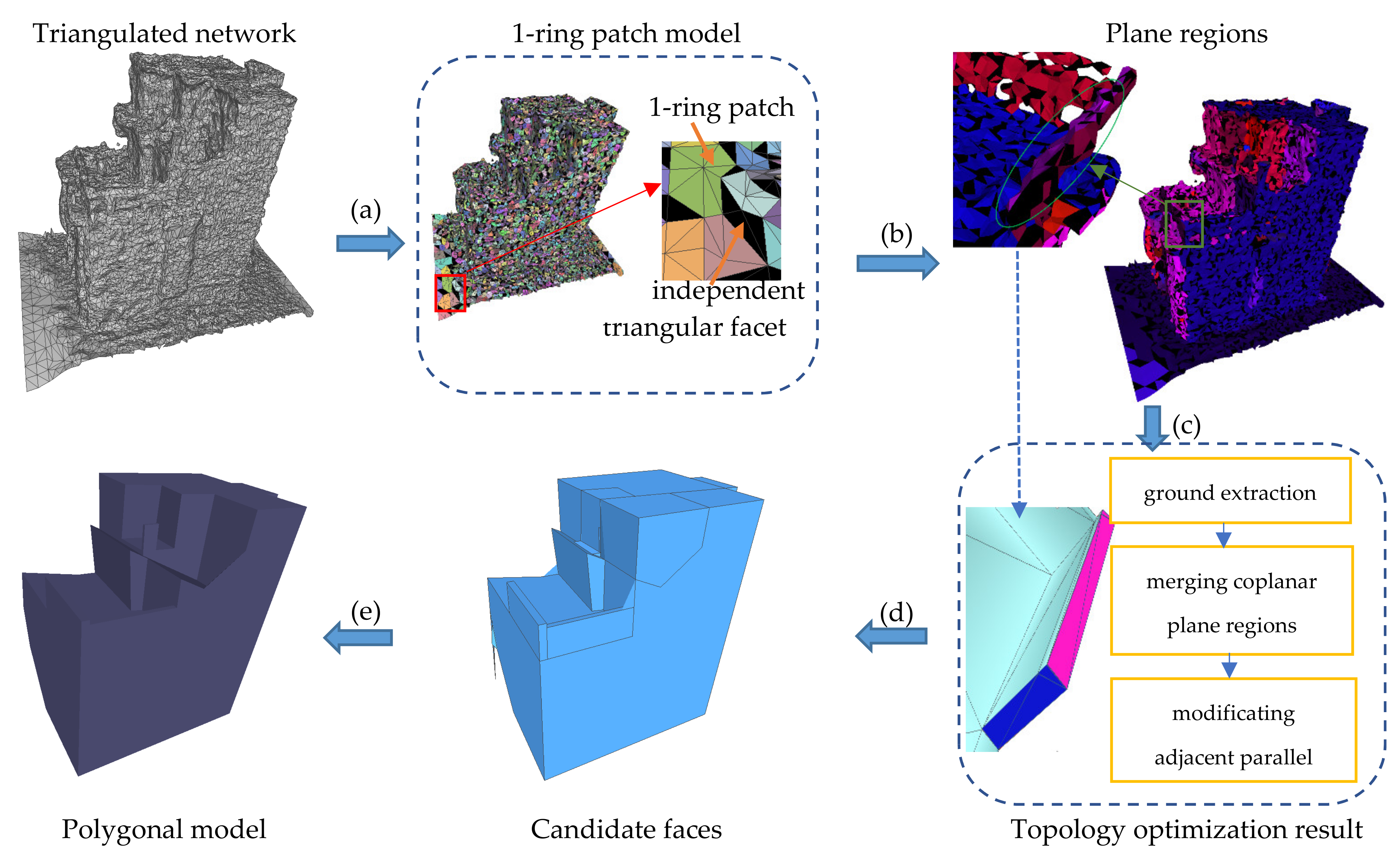
As shown in Figure 1, the method in this paper mainly includes five steps: (a) converting triangular mesh model into the 1-ring patch model, (b) extracting plane regions based on region growing of the 1-ring patch model, (c) building and optimizing the topology of the plane regions, (d) generating candidate faces, and (e) selecting candidate faces to obtain the polygonal model. The framework of generating a polygonal model from the mesh model is derived from significant improvements to SABMP. In step (a), the proposal of the 1-ring patch primitive replaces the original processing unit for subsequent steps, typically step (b). In step (c), several well-designed rules are introduced into the topology optimization process, such as ground extraction, coplanar plane regions mergence, and adjacent parallel planes modification. Other minor improvements beyond SABMP include the use of the hierarchical index in calculating the 3-ring planarity in step (a) and the use of the divide-and-conquer split strategy in constructing the building scaffold in step (d).
2.1. The Generation of 1-Ring Patch Model
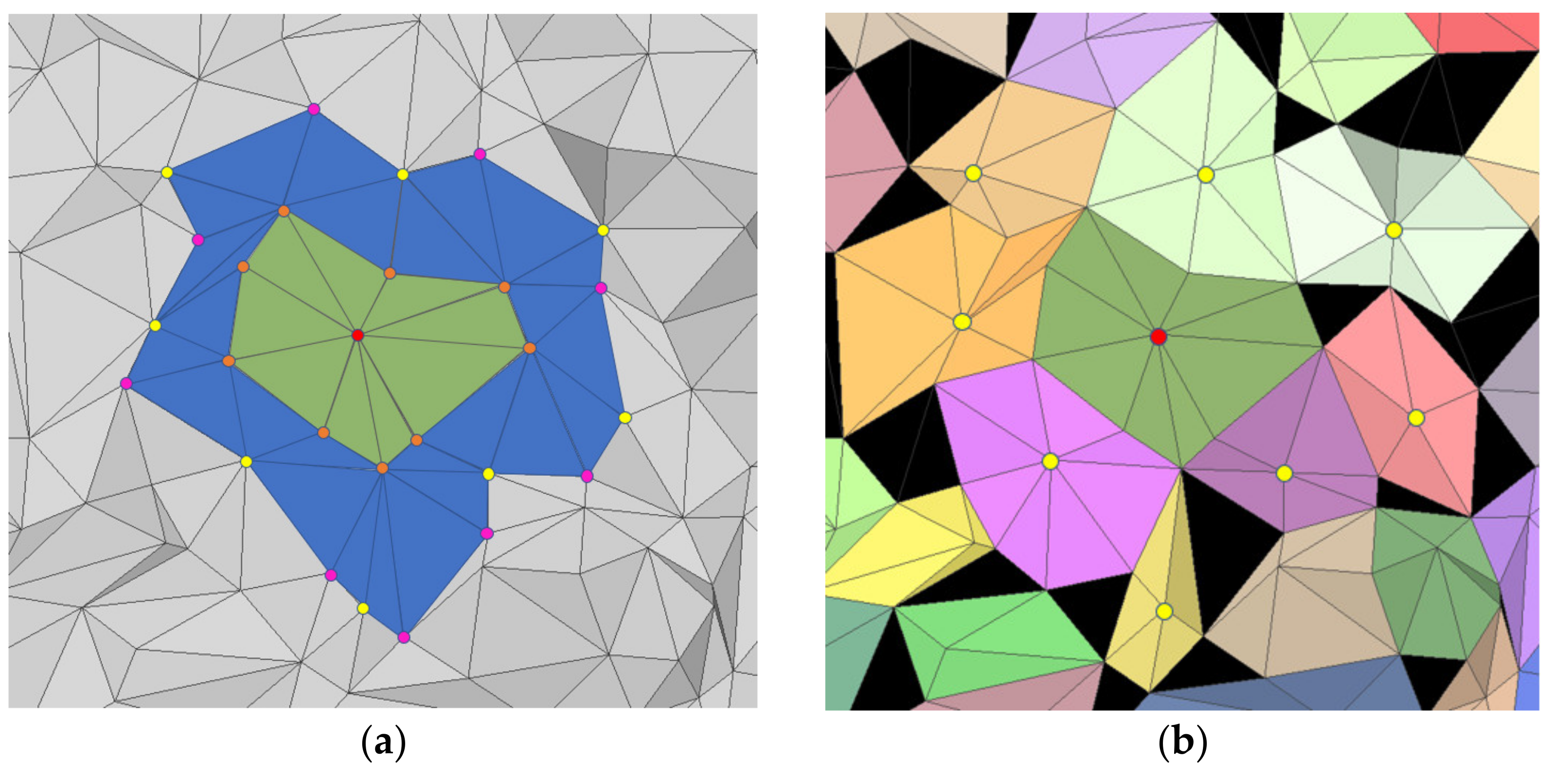
The choosing of model primitive type is a critical step for mesh polygonization. Usually, as the smallest planar primitive of mesh, the triangular facet represents the local geometric feature; thus, it is the most widely used primitive for mesh processing. Vertex position, vertex normal, and plane normal of triangular facets are important geometrics for the mesh model to perform filtering, segmentation, classification, etc. The fidelity of the triangular mesh is high when the mesh model is not noisy. However, the building mesh model generated from MVS contains lots of noise in many cases, and the mesh of the building surface that should be highly planar is rugged. In this case, a single triangular facet performs poorly in characterizing the features of the local region. Taking account of a better balance between feature expression ability and calculation efficiency, instead of a single triangular facet, a type of super face called 1-ring patch is used as the basic primitive for geometric feature expression. Our inspiration comes from the region-growth strategy based on the planarity of the k-ring neighborhood [36]. A 1-ring neighborhood refers to the set of all vertices connected with a vertex by an edge in a triangular mesh, while 1-ring patch refers to the super face formed by all the triangular facets containing this vertex. As shown in Figure 2a, the 1-ring patch (green region) consists of a center point (labeled in red) and its surrounding boundary points (labeled in orange), and its geometric features, which are more representative of local information, include the position, planarity, and normal of the patch. The patch model generation process is as follows:
- Calculate the k-ring planarity of all the vertices of the mesh model and add the vertex with the greatest planarity to the list of new center points (labeled in red).
- Construct the 1-ring patch of the center point. The 1-ring neighborhood points of the center point are taken as the boundary point of the patch, the centroid of the patch is calculated as its position, the normal of the center point is taken as the normal of the plane, and the planarity of the center point as its planarity. Remove the center point from the list.
- The 2-ring neighborhood points (labeled in yellow and pink) of the center point are as added to the list of new center points (labeled in yellow). The point labeled as a boundary point (labeled in pink) in the patch generation process should be removed from the list.
- Repeat steps 2 and 3 until the entire mesh model is traversed. The result is shown in Figure 2b where patches are labeled in different colors.
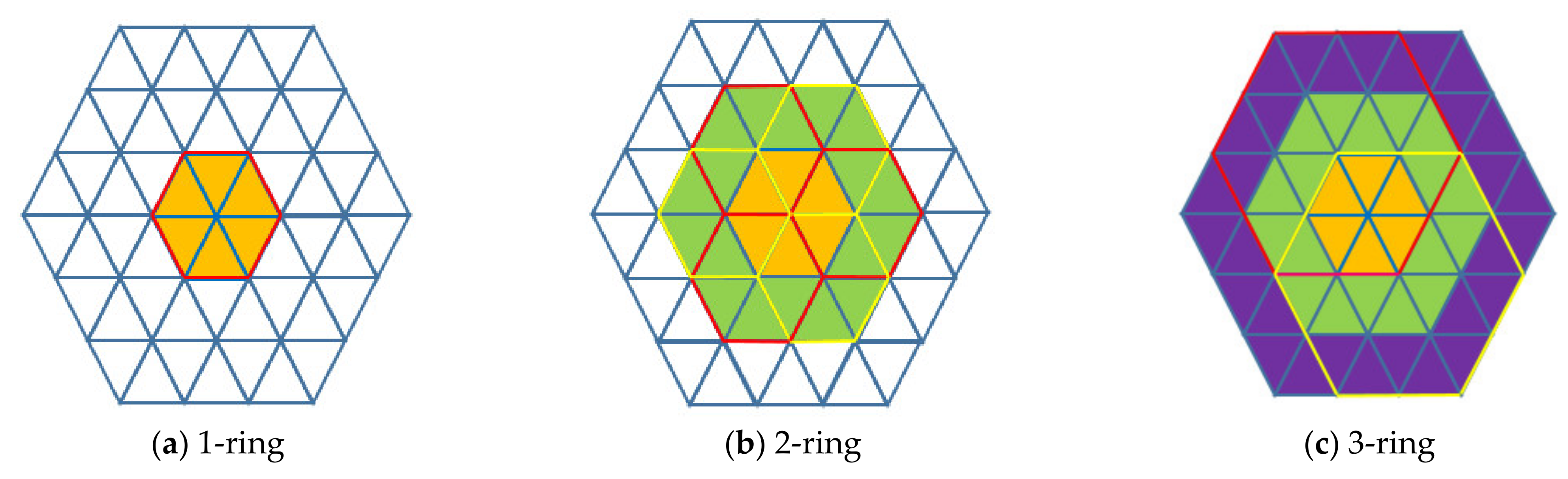
In step 1, we adopt SABMP’s conclusion that ring neighborhoods of order 3 outperform other orders. To speed up the calculation of 3-ring planarity, we propose a strategy based on a hierarchical index. Different from SABMP and other traditional methods traversing the k-ring neighborhood of each vertex directly, our method constructs the index relationship of ring neighborhoods between high order and low order and avoids the repeated search of neighborhood points. As shown in Figure 3, the k-ring neighborhood of a vertex can be represented by a set of the k-1 ring neighborhood, whose center point is the 1-ring neighborhood point of that vertex, and we can use the established hierarchical index to obtain all the k-ring neighborhood points.
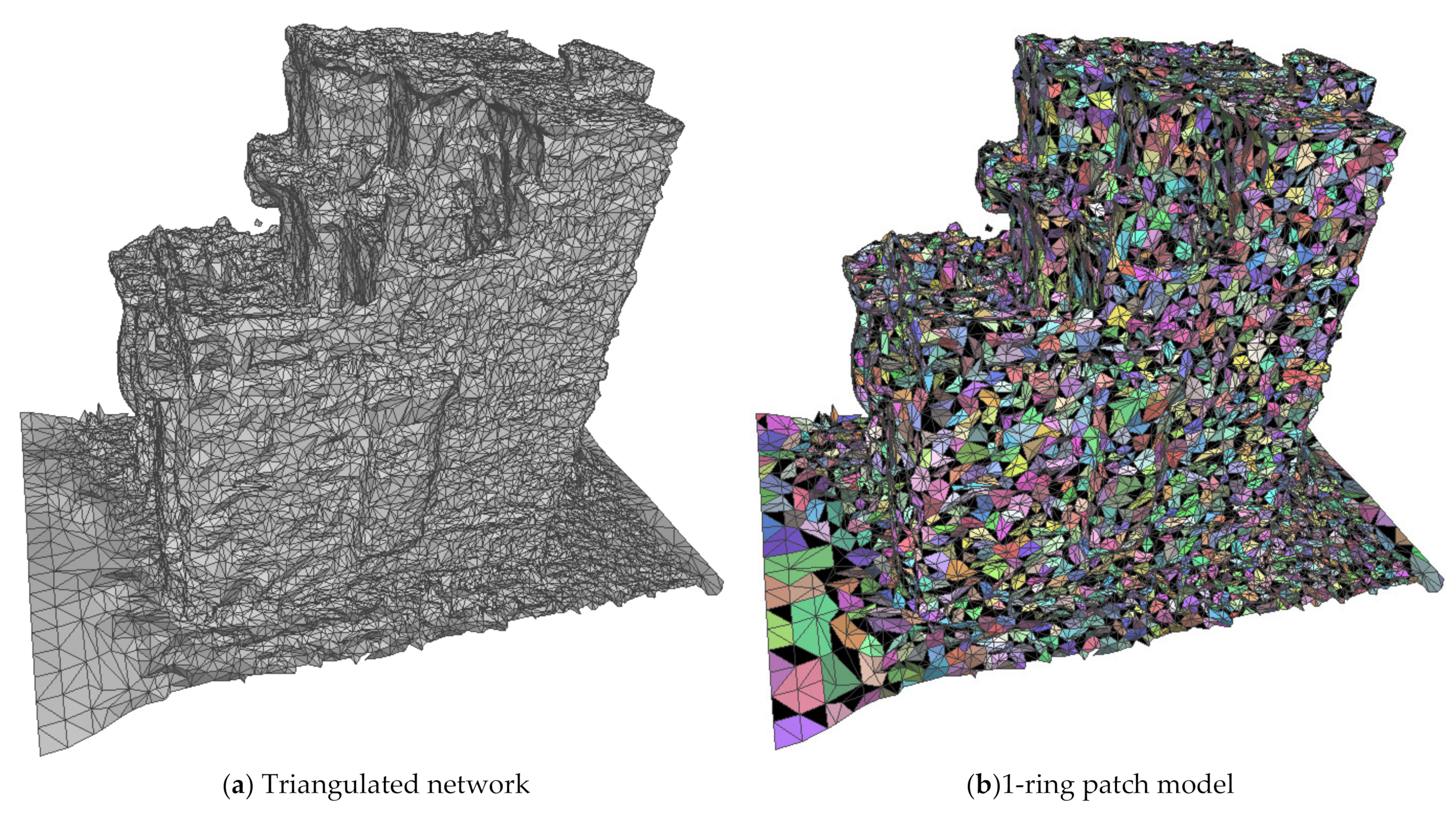
As shown in Figure 4, the final reconstructed surface model consists of inter-connective 1-ring patches and independent triangular facets that are not contained in the patches. Although it is a hybrid model represented by two types of primitives, we still call it the 1-ring patch model. The reason is that we want to emphasize the characteristics of this model and that the 1-ring patch primitive does occupy a dominant position compared to the independent triangular facet. Patches and triangular facets could share boundary points, and the adjacency between patches is determined by the 2-ring adjacency between their center points. Using the 1-ring patch to reconstruct a triangulated net, the building surface can be represented with fewer elements while keeping the original geometric information.
2.2. Region Growing
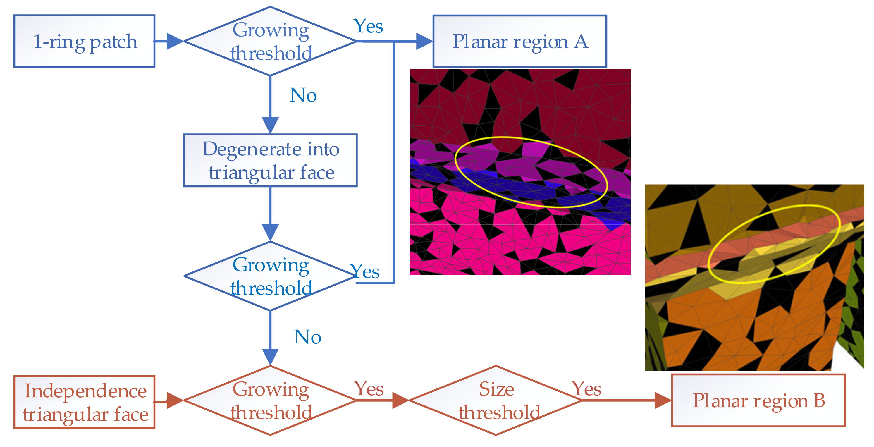
Restricted by the data quality of the MVS mesh, the planar structure of the building may be rugged, and the boundaries between different plane regions are difficult to distinguish. Therefore, based on the mesh model composed of 1-ring patches and triangular facets, a two-step strategy of rapid region growth is designed: region growth of patches and region growth of triangles (shown in Figure 5).
The first step of region growth of patches is selecting the patch with the greatest planarity as the seed point. The growth plane is then initialized by principal component analysis on the vertices contained in the patch. For the growth judgment of its neighborhood patch, both distance and normal direction threshold are used to improve the segmentation accuracy. If the growth of the neighborhood of the seed point fails, our method degenerates the patch into several triangular facets and recalculates the distance between the vertices of the triangular facet and the growth plane and the angle between the normal of the plane and the normal of the triangular facet. It should be noted that, due to the different growth spans of patches and triangular facets, different normal direction thresholds (anglepatch and angletri) are adopted, and the triangular facet cannot be used as the seed point of patch region growth. The distance threshold is a statistic that needs to be adjusted sometimes.
where is the length of the edge of the triangulated network, is the number of edges in the triangulated network, and is the adjustment coefficient, which is 1 by default.
After the traversal of all the patches, many patches, without joining to any plane region, degenerate into triangles. These facets generally present as some slender strips or debris, which cannot be ignored for their importance of structure expression, so it is necessary to carry out the secondary growth of triangular facets. A seed facet was randomly selected from these facets, and the growth was carried out according to a certain distance and normal direction threshold until all the degradation facets are added to some plane regions that must have enough faces (size threshold = 10).
The growth of patches is the main step of mesh segmentation, and the growth of triangular facets is the necessary supplement of patches growth. After the two-step growth, the main plane regions of the building are extracted as some sets of patches, and the connecting regions between the planes are precisely distinguished in the form of triangles. It should be noted that, within the plane region, the triangular facets that do not degenerate from patches will not grow as the initial seed, but it may be added to a plane region in the process of triangle growth, to consider the accuracy and efficiency of segmentation.
2.3. Topological Optimization
Since the neighborhood relations of 1-ring patches have been established during the remodeling process, the topology graph of the building plane structure can be easily constructed according to the plane region extracted from the regional growth. Since the mesh may be noisy and the topological relations of all the building planes cannot be guaranteed to be fully correct, we need to optimize the initial topology further. Topology optimization includes the deletion of redundant planes, the addition of missing planes, and the modification of the adjacency relation, which is mainly divided into three stages: (1) ground extraction, (2) the merging of coplanar plane regions, and (3) the modification of adjacent parallel plane regions.
2.3.1. Ground Extraction
Since our work focuses on the reconstruction of the single building model, extracting a single building from a large scene is beyond the scope of this paper. Related scholars have done a lot of research on building extraction, but it is still difficult to extract clean buildings in many cases [37,38,39]. In addition, the polygonization algorithm requires an input of a closed model or a model surrounded by the ground to ensure the two-manifold. To make our approach more versatile, a step clustering the regions around buildings into a ground plane region is specifically designed for our polygonization approach.
In our research scenario, the whole mesh can be simply summarized into three main types: the ground, the building façade, and the building roof surface. The building façades are generally perpendicular to the ground, and in some cases, they will also be at a certain degree of an angle with the vertical direction. Roof surfaces of the building are generally divided into two categories, horizontal and oblique. In this paper, we focused on the common architectural forms, and some relatively unique architectural designs were not in our consideration. Therefore, according to the angle between the plane and the horizontal plane, they can be roughly divided into two parts, building façades and horizontal planes. Moreover, the candidate ground planes are extracted from the horizontal planes, according to their elevation difference with the centroid of the adjacent building façade (less than disground).
The candidate ground plane with the lowest elevation is taken as the seed plane, and other non-building planes are extracted through a standard region-growing process. In this paper, the planes that need to be taken as the ground plane can be divided into three main categories, and corresponding different strategies are designed to merge them with the seed plane:
- Candidate ground plane. If the height difference between the seed plane and the candidate ground plane is less than the common floor height (hf), it will be labeled as the ground and merged with the seed plane to update its elevation.
- Non-façade neighborhood plane. A normal direction threshold anglenonbd is used to determine whether the neighborhood plane was a non-façade plane. The non-façade plane region with a limited area (area < areanonbd) should be included in the seed plane. Since these planes are generally non-ground features, they do not participate in the update of ground elevation during the growing process.
- Sub-ground plane. Planes that are lower than the seed plane or less than half a floor height (hf) above the ground are merged with the seed plane. These planes also update the neighborhood of the ground plane without recalculating the ground elevation.
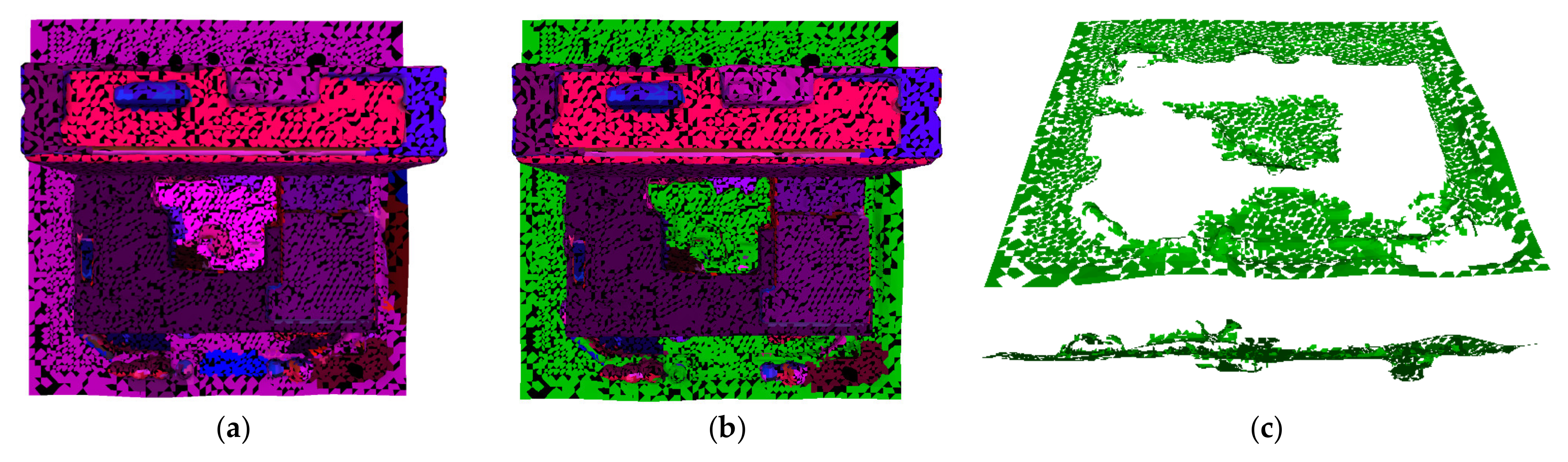
As shown in Figure 6, the ground region is extracted, and the number of plane regions to be polygonized decreases from 264 to 190, which could make the subsequent optimization simpler and more efficient.
2.3.2. The Merging of Coplanar Plane Regions
Since the regional growth is performed according to the adjacency and the artificial threshold value, some extracted planes are inevitable coplanar but not merged. It is easy to fail during the generation of the polyhedron model in this case, so these regions that are supposed to be in the same plane should be merged. SABMP [23] traverses all plane regions and merges the approximately parallel plane regions with small spatial distance into a new plane region. And the entire traversal process is repeated until no new region is created. To improve the processing efficiency, a “merging the biggest” strategy is adopted so that the entire traversal process only needs to be executed once. The process is executed as follows:
- (a)
- Sort the plane regions according to the number of patches, choosing the biggest plane region as the seed region to annex other regions.
- (b)
- Traverse all the regions smaller than the seed region and calculate the angle and distance between two planes regions. The angle threshold anglemerge and distance threshold dismerge are used to determine whether a pair of plane regions are coplanar and should be merged.
- (c)
- For a pair of coplanar regions, merge the smaller region into the seed region, otherwise choose the next largest plane region as the seed region.
- (d)
- Repeat steps (b) and (c) until all the regions are traversed.
2.3.3. The Modification of Adjacent Parallel Planes
Since the plane obtained by our region growth is a directed plane, that is, the normal always point to the outside of the model, it is necessary to optimize their topological relations according to the orientation of the normal of the parallel plane. For adjacent parallel planes with the same normal direction, our method deletes their edge in the topology graph. Adjacent parallel planes opposite the normal vector are generally some long and narrow independent structures on the building, such as the parapet, billboard, fence, and so on. They occupy a small proportion of the space but are very important for the restoration of the real appearance of the building.
In a normal topology, there should be no adjacency between parallel planes. However, for some parallel planes with small spatial distances, regional growth is difficult to ensure that there will be no adjacency relationship between the patches or triangular facets. When they do not conform to the coplanar property, their topological relations must be modified to avoid structural degradation of the polyhedron model. In this case, an algorithm is proposed to correct the topological relationship by rebuilding the missing connection planes between parallel planes.
First, we selected the interconnected patches in two parallel planes for connectivity analysis, and a candidate region with the largest number of patches was selected after dividing them into several independent regions. Then, we selected the plane region with a smaller patch number from two parallel plane regions and calculated its bounding box. The patches of the candidate area were sorted in order from high to low, and patches were selected successively as the face elements of the connection plane.
where and represent the bounding box range in the x and y direction, respectively. After the construction of the horizontal connection plane, add its adjacency relationship to the topology graph.
The vertical connection plane may also need to be rebuilt depending on the neighborhood of the horizontal connection plane. In addition to two parallel planes, the adjacency of the horizontal connection plane may also include the neighborhood of two parallel planes. If the normal vector of the neighborhood plane is horizontal and not inside the parallel plane bounding box, it is also considered to be a neighborhood of the horizontal connection plane. The number of vertical connection planes to be constructed is , where is the number of neighborhoods of the horizontal connection plane. A similar approach is taken to the horizontal connection plane, selecting patches to construct the vertical connection plane along the horizontal direction, in order.
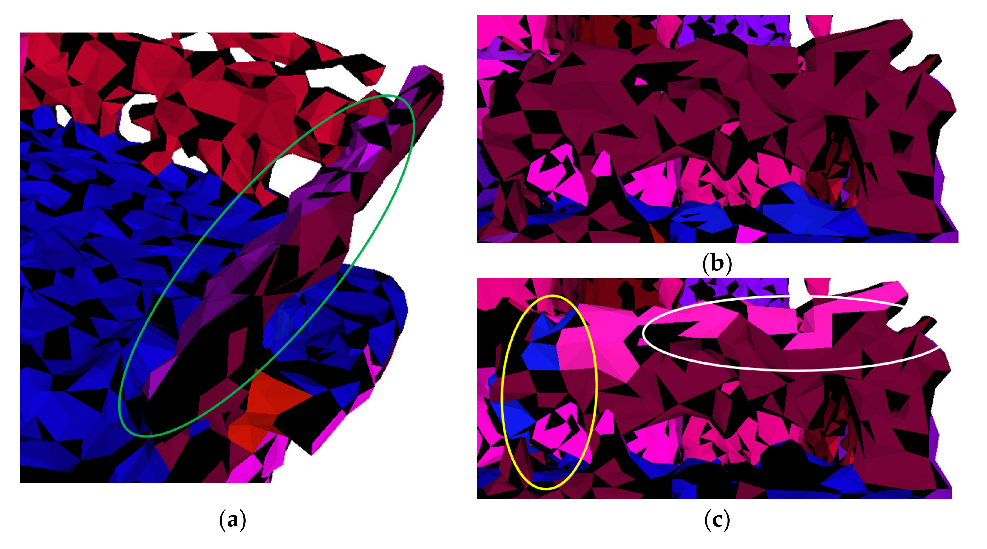
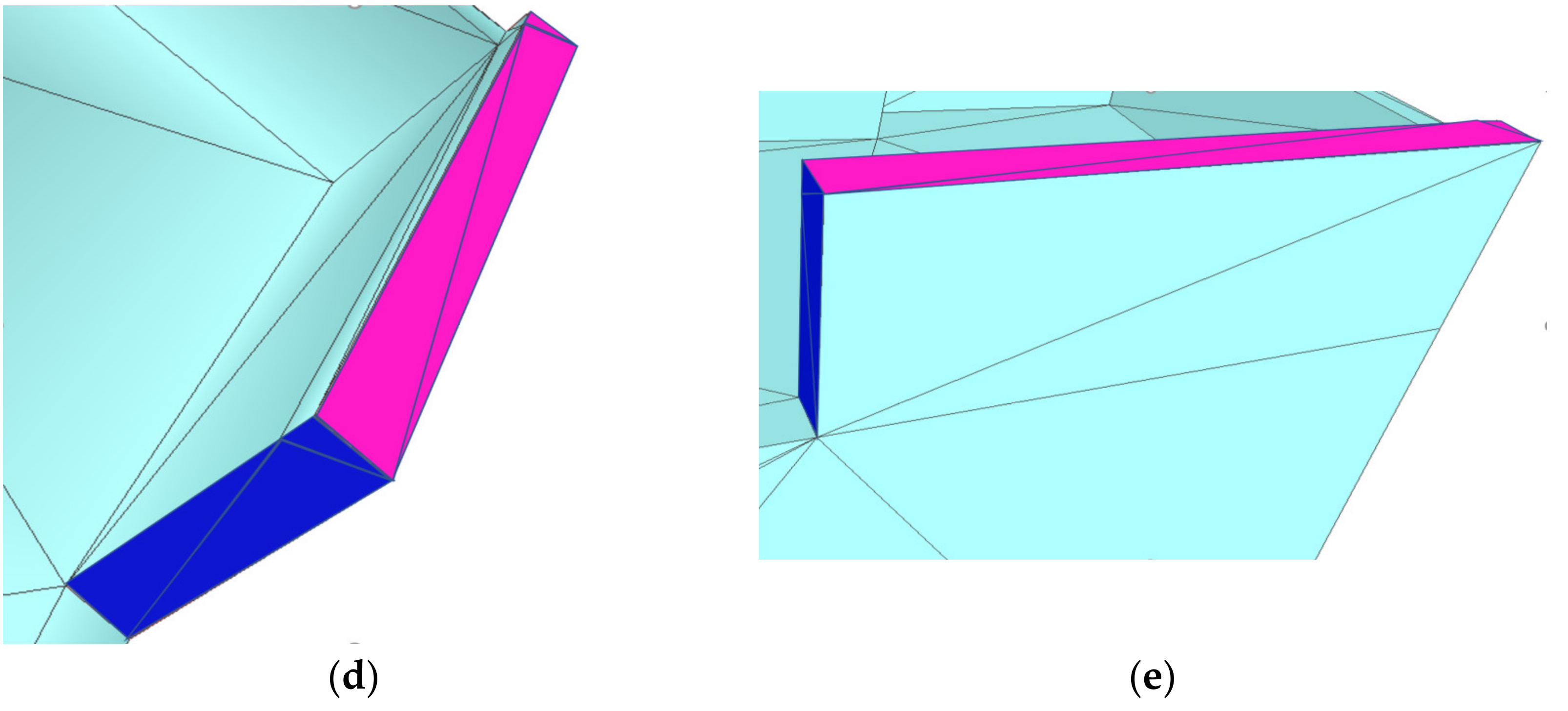
where are the bounding box range in the height direction. The normal vector of the vertical connection plane is equal to the cross product of the normal vector of the horizontal connection plane and one of the two parallel planes. In addition to two parallel planes and the horizontal connection plane, its neighborhood should add the adjacent horizontal plane of the smaller parallel plane. As shown in Figure 7, the direct connection of parallel planes can be avoided after the rebuilding of the connection plane. In the current stage, our work does not deliberately pursue the authenticity of the segmentation results, but the rationality of the topology structure is guaranteed.
In addition to the above important optimization measures, our work also performed other topology optimization work, such as deleting the region with less than three adjacent planes that cannot build a normal polygonal model.
2.4. Generation of Polyhedron Model
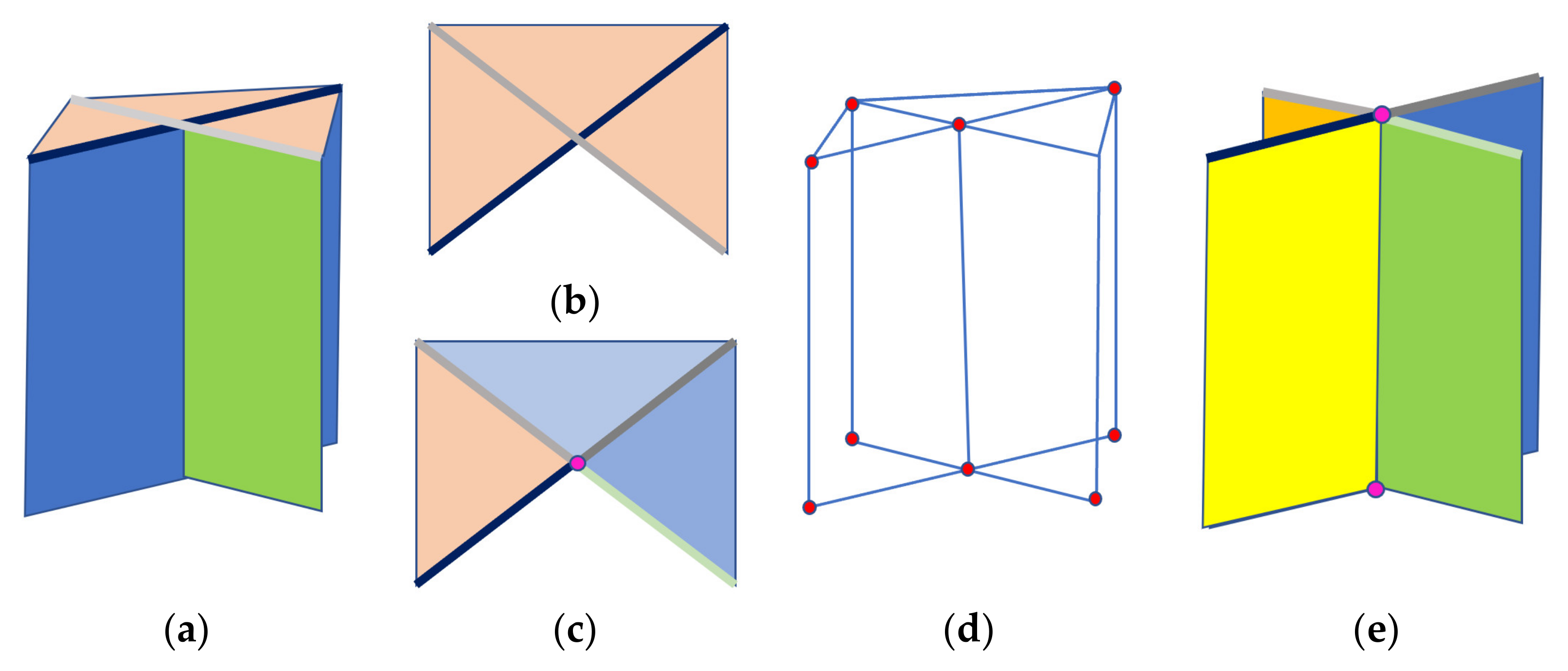
Based on the topology optimization, the number of nodes and edges of the topology graph was reduced considerably, and also the topology quality was improved. In the next step, taking the optimized topology graph as input, a polygonization process of improved efficiency is implemented with the consideration of the independence between plane regions. Building scaffold refers to the connection graph made up of the plane edges formed by the intersection of two support planes and the corners formed by the intersection of three support planes [19]. According to the adjacency relation of the plane regions in the topology graph, it is easy to calculate the intersecting edges and points. The problem that some adjacency relations cannot be restored correctly in the topology graph causes some corners to not be able to be found. To obtain the correct building scaffold, SABMP traverses all line segments to check the coplanar relationship and intersection relationship between two pairs. For the edges that meet the intersection conditions but lack intersection points, the line segments are split from their intersection points, and the intersection points are added as new corners. Whereafter, all line segments are traversed over again. The schematic diagram is shown in Figure 8.
A line segment has more than one support plane and the intersectant line segment lies on one of the support planes. In Figure 8a, the blue face is the support plane of the black segment, while the green one is the support plane of the gray segment, and the orange one is the common support plane of the pair of line segments. The split of a line segment is the split of the plane region where the line segment lies and does not affect the line segments of other plane regions.
Therefore, a divide-and-conquer split strategy was adopted for each plane region. In the first step, this strategy established a subordinate relationship between the plane region and the line segment and then carried out a relatively independent split process for each plane region. In addition, all the checked line segment pairs were marked and did not repeat splitting. The pseudo-code of our strategy is shown in Algorithm 1. Under our improvement, the time complexity of the algorithm was reduced from to , where is the number of splits, is the number of line segments, and is the number of plane regions.
| Algorithm 1. Refine edges. |
| Input: The set of edges of each plane Output: The refined edges and the final corners 1 while do 2 3 for do 4 for do 5 for do 6 if then 7 8 if then 9 10 11 if 12 then 13 14 15 split, split 16 17 18 go to line 1 19 end if 20 end if 21 end if 22 end for 23 end for 24 end for 25 end while |
Using the projection of the building scaffold into the planar regions, we could obtain the candidate faces for the simplified mesh, as shown in Figure 8e. Considering the influence of false segmentation and the requirement of water tightness, a further step to determine whether a candidate face should be preserved was adopted using the method in SABMP.
After the optimization process, the simplification result of the model could be obtained, and the watertight and manifold characteristics of the polyhedron model were ensured.
3. Results
3.1. Topological Optimization Effect
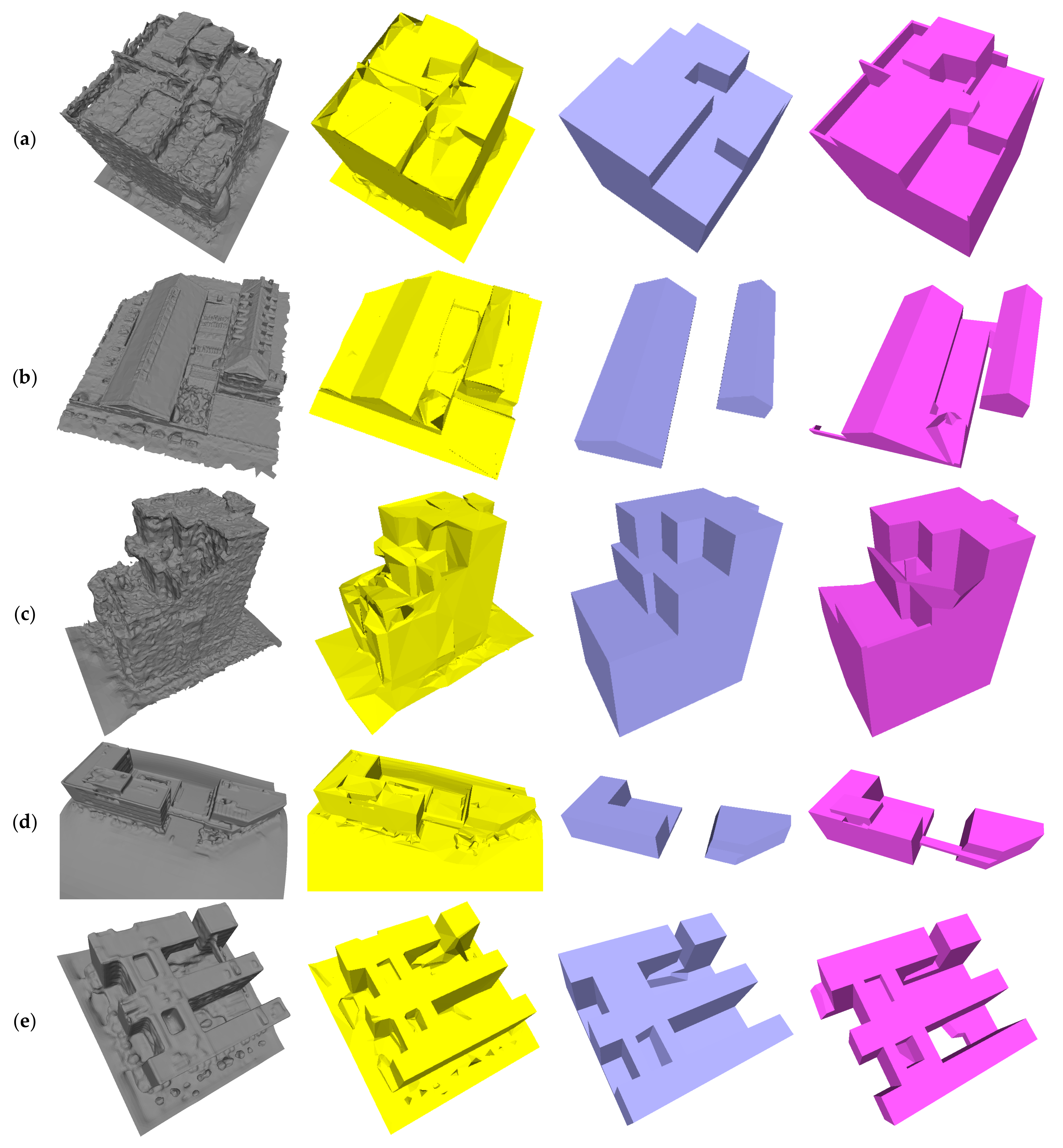
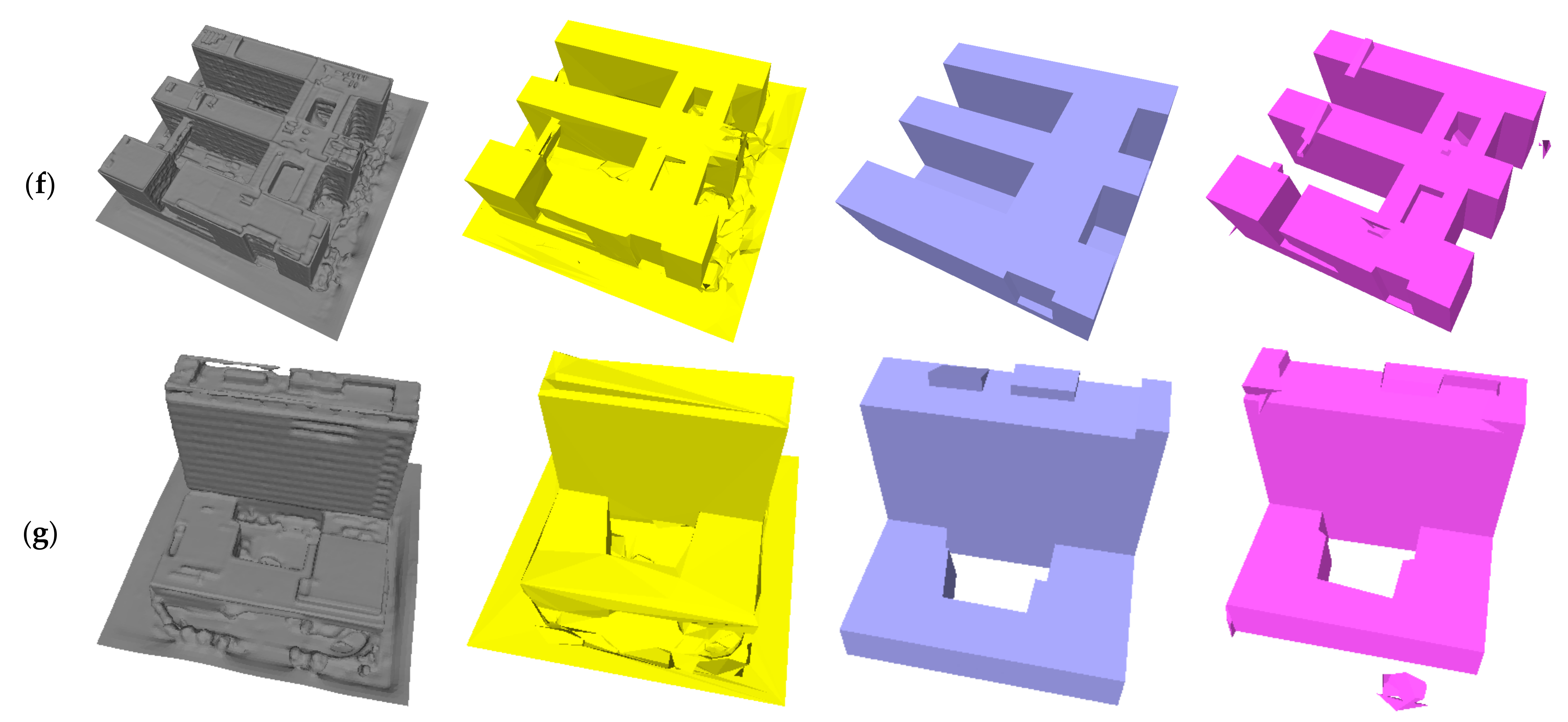
To intuitively reflect the effect of topology optimization, we show the modeling results of several building mesh models processed by our method in Figure 9, and we compared them with the results of two other polygonization methods.
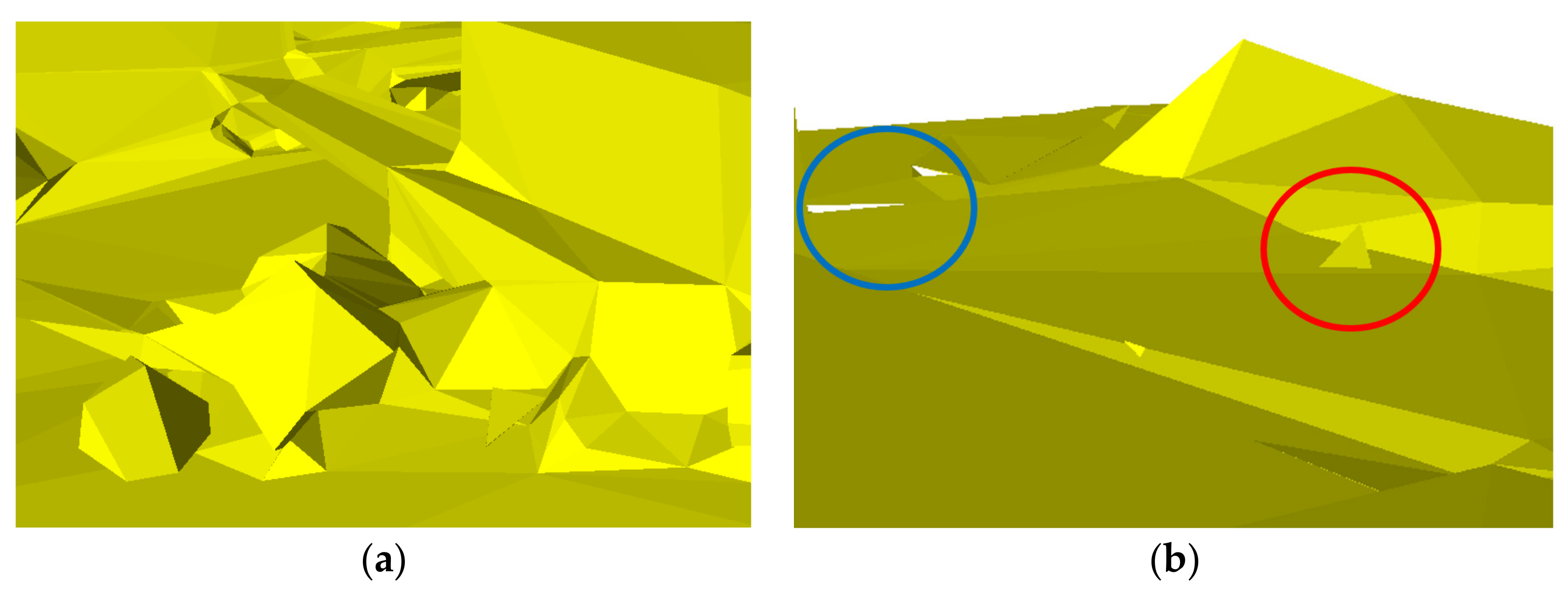
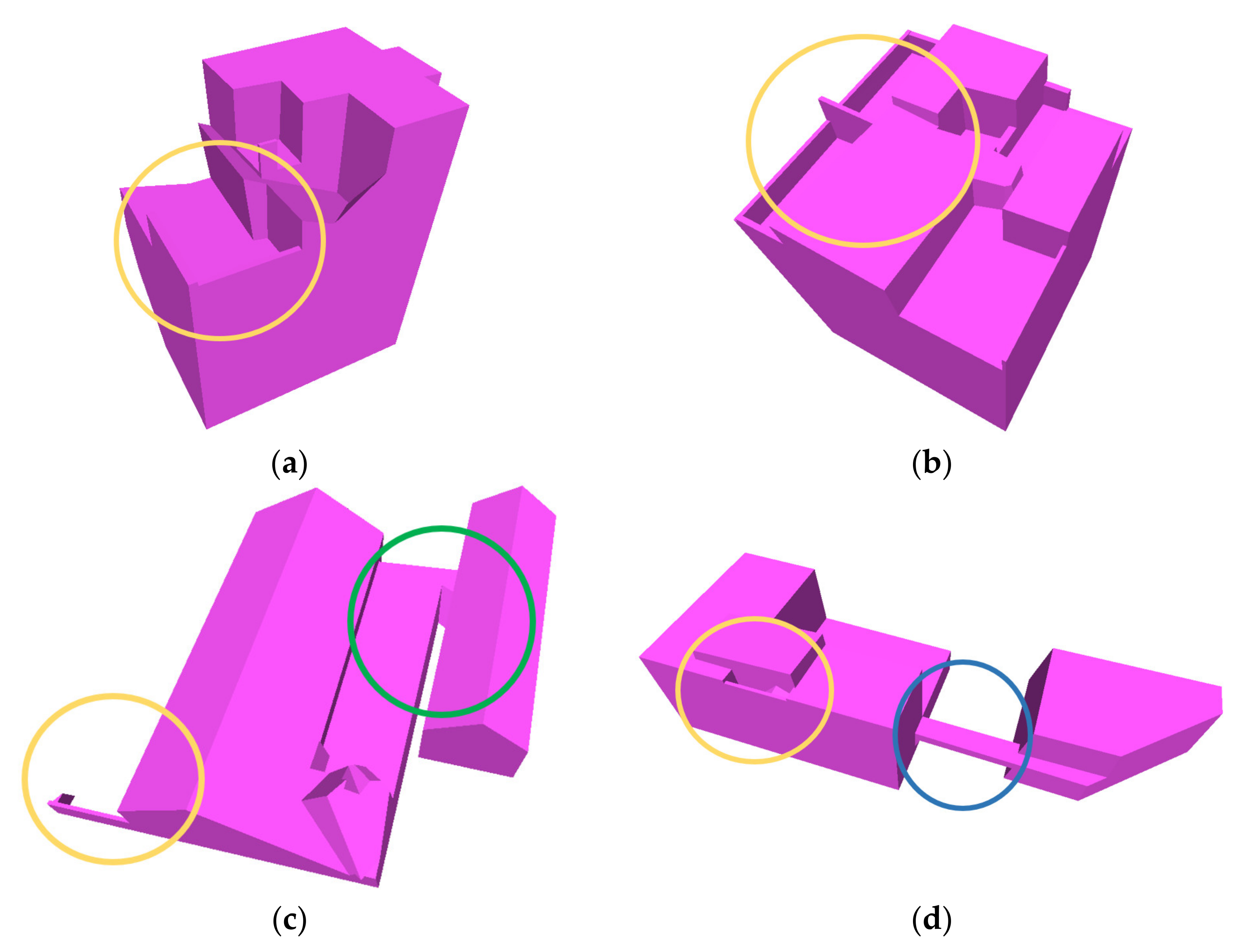
The input data used in the experiment are all the monomer building mesh models created by the MVS method with relatively significant noises, including the noise on the building (e.g., model (c)) or ground (e.g., model (g)). These buildings are structurally complex: the roof of model (a) has a large number of parapets; model (b) has a narrow gap between the building blocks and a large irregular structure; in model (d), two buildings are connected as a whole through a dangling corridor; model (e) and model (g) are annular structures. After topology optimization, the main structure and important details of the building could be restored, and the watertight manifold polygonal model composed of a few planes was generated. In contrast, the VSA method does not guarantee watertightness, and many non-architectural details were retained, as shown in Figure 10. Due to the correct recovery of topological relations, the results in this paper can retain the long and narrow details that are easy to be omitted and avoid the structure degradation caused by topological errors (see Figure 11 for more details).
As illustrated in Table 1, the polygonal model greatly compressed the size of data. Because our model retained more details, the number of faces was slightly larger than the result of SABMP, such as models (a), (b), (c), etc. For model (e) and model (g), there was little difference in the level of model detail obtained by the two methods, and our results were more concise. Taking model (f) for example, where the input model is a 19.1MB OFF file (which also supports other formats such as PLY, OBJ, etc.), our method produced an 8.3 KB PLY file, compared to 218 KB for VSA and 4.2 KB for SABMP.
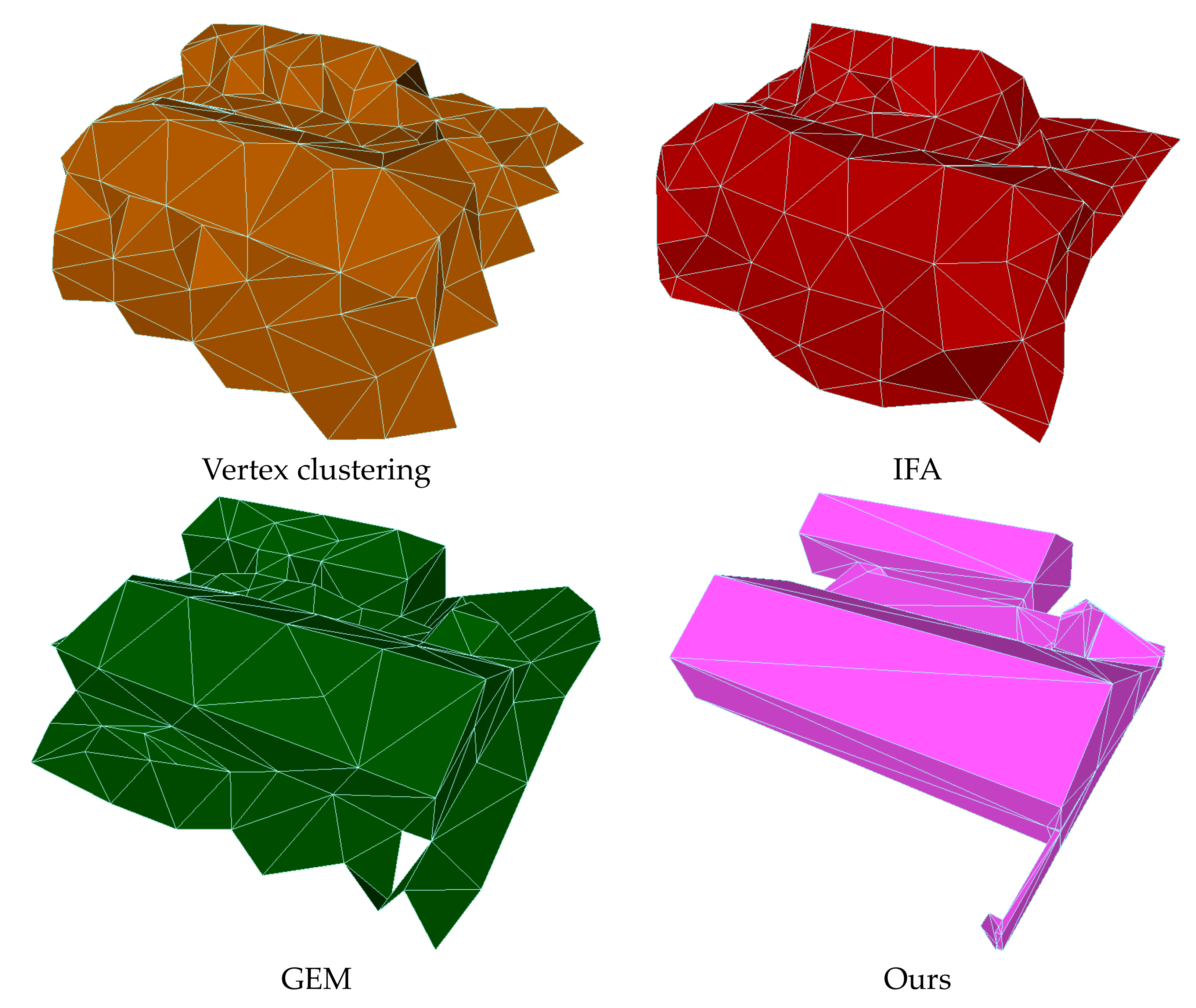
The methods based on mesh element deletion could not guarantee the manifold and watertightness of the results and did not compare well with our method in maintaining the main structure of the building. Under the condition of maintaining the same number of triangular facets, we compared the simplified results of the vertex clustering method, QEM method, and IFA method with our method, as shown in Figure 12. The experimental results of the vertex clustering method and QEM method were achieved by MeshLab [12].
3.2. Model Accuracy
Hausdorff distance [40] is generally used to evaluate the accuracy of mesh simplification. Many scholars use the distance between the sample point of the simplified model and the original model to evaluate the accuracy. This method cannot reflect the degree of detail loss of the simplified model. Therefore, our work used the Hausdorff distance from the original model sampling point to the simplified model to reflect the important structure retention capability of the method presented in this paper.
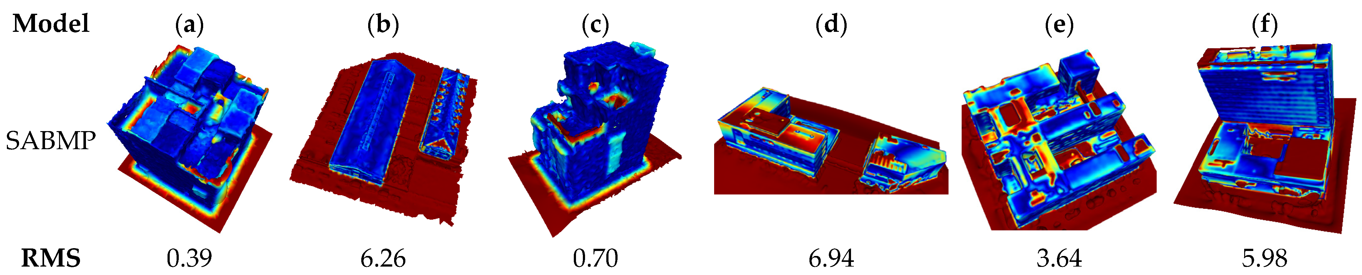
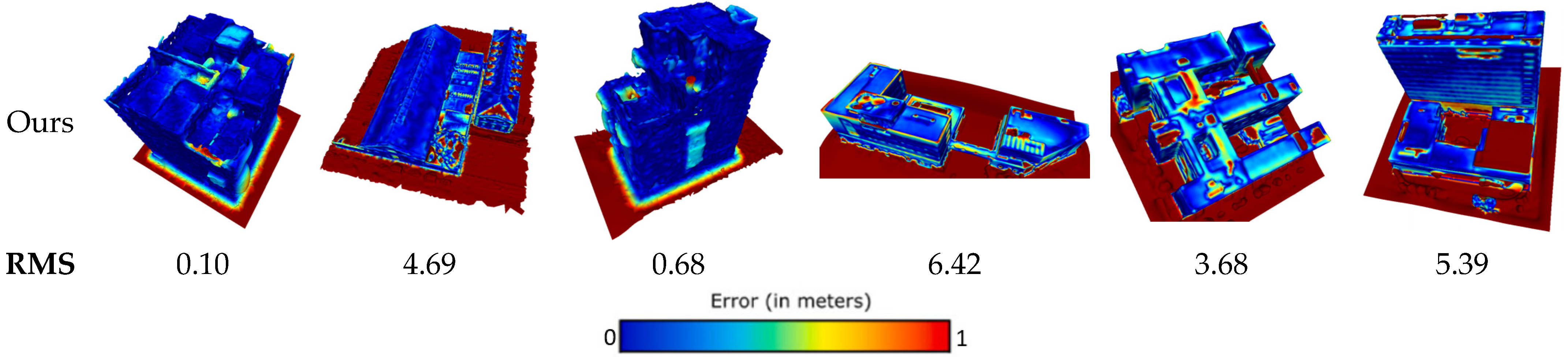
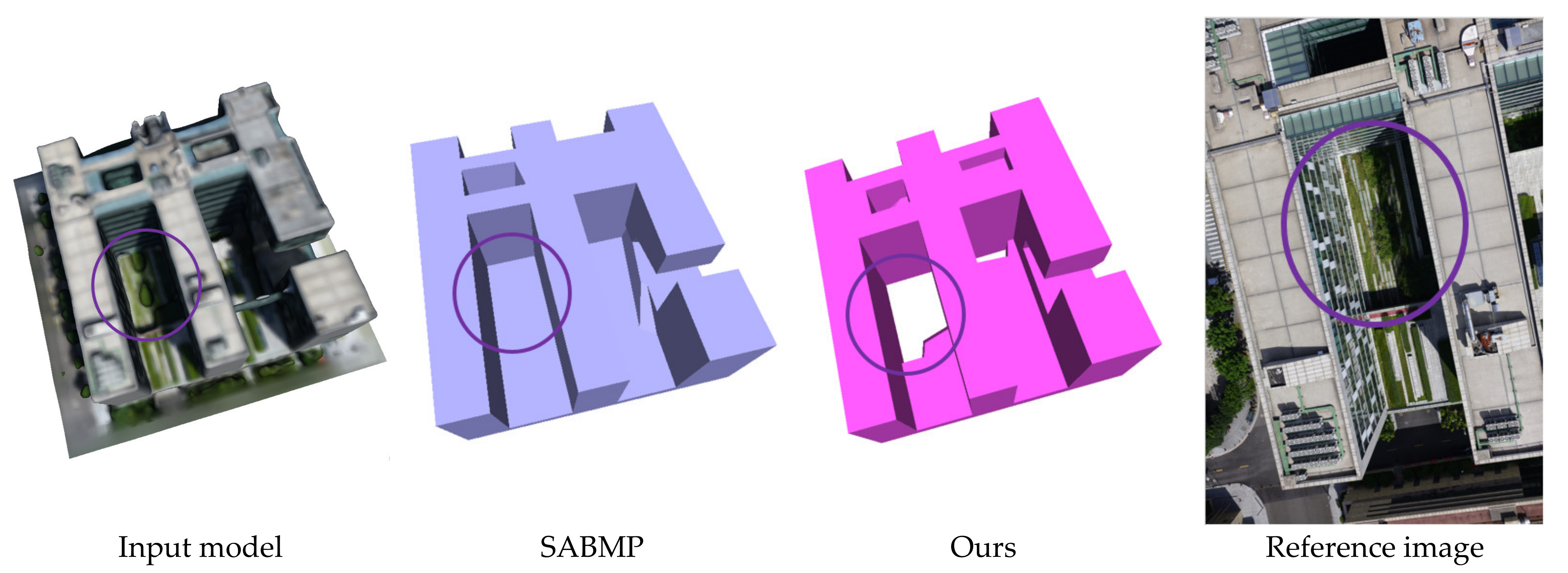
The results are shown in Figure 13, where the red regions surrounding the building represent the ground. Since the ground would not be retained in the simplified model, the Hausdorff distance in the ground region was relatively large, which led to a larger root mean square error (RMS) value. In consideration of no ground filtering process in SABMP, to be fair, the ground region was also included in the calculation of RMS in the method in this paper. It can be seen from the figure that the RMS value of the proposed method was less than that of SABMP because the degradation of the building structure was avoided, and the quality of the simplified building model was significantly higher than that of SABMP. The RMS value difference of model (e) was small because the method in this paper correctly distinguished the building region from the ground region, which increased the RMS value. As can be seen from Figure 14, our model is similar to the real building.
3.3. Efficiency Optimization Effect
While improving the effect of the model, our work also made improvements to the efficiency in several stages. We compared the running time before and after efficiency optimization of each stage one by one, as shown in Table 2. All experiments were performed on a mobile workstation with a 2.30 GHz Intel(R) Core (TM) i9-9880H CPU and 64 GB RAM. We have implemented our method in C++ with the CGAL library [41] for mesh operation and Boost library [42] for topology operation.
To realize the efficient conversion from the mesh model to the polygonal model, our method optimizes the efficiency of four main processing steps. In the comparison experiment, some steps, such as plane extraction and topology optimization process, were compared with SABMP. The output of some steps was quite different from that of SABMP, so a direct comparison was not appropriate. We compared the running time before and after efficiency optimization in these steps, such as planarity calculation and polygonal model generation.
The 1-ring patch model conversion was an additional step added in the planarity calculation process, so the running time of this step without efficiency optimization was longer than that of SABMP. After the calculation method of 3-ring planarity was improved, the consumption time was reduced by half, which was also less than that of SABMP.
In the part of plane extraction, region growth was carried out based on 1-ring patches. Compared with SABMP, the processing speed was improved by 5–10 times. The reason for the fluctuation of the speed improvement performance is that the optimal growth thresholds of different building models were different in SABMP.
Due to the improved merging algorithm of the coplanar plane region, although several optimization operations were added in the topology optimization stage, the speed was improved compared with SABMP. The efficiency promotion was positively correlated with the number of planes that needed to be merged, ranging from 8 to 800 times.
The subdivision process of candidate faces was improved, and the polygonization time was reduced for the input topology of the same planar region. Model (f), in particular, improved the processing speed by 10 times due to its finer mesh and more candidate faces need to be subdivided. Our method did not improve significantly compared with SABMP because the running time of the polygonization process is related to the complexity of the simplified model, and one of the purposes of topology optimization in this paper was to maintain the complexity of the model.
Decided by the complexity of the mesh model, the efficiency improvement of the whole process varied from 10 to 200 times. In our experiment, there was approximately a linear relationship between the running time and the face number of input data. The number of faces processed per second was about 60,000, which is better than SABMP in both efficiency and stability.
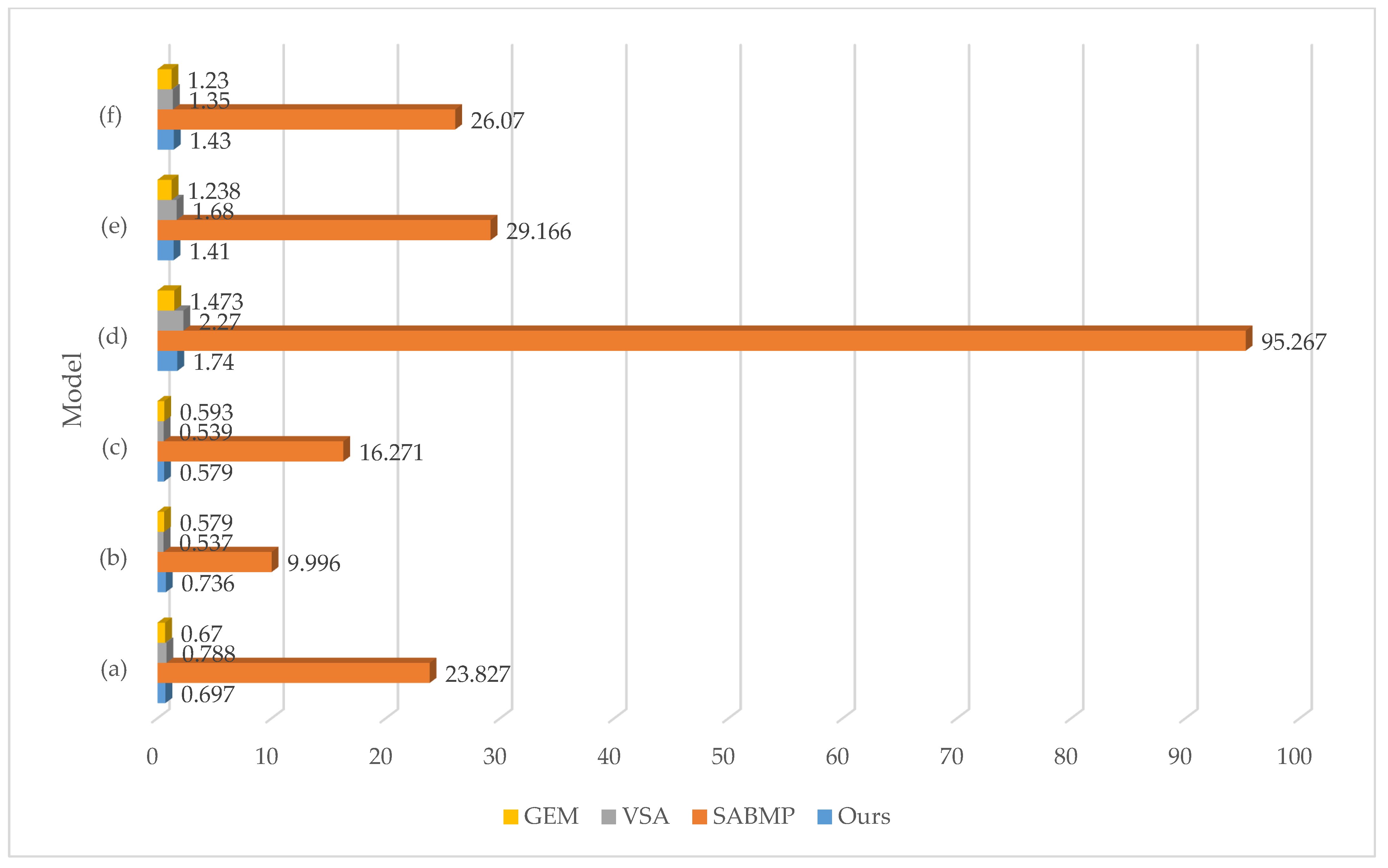
To show the effect of efficiency optimization more intuitively, we compared the time consumption of the SABMP method, GEM method, VSA method, and the method presented in this paper in Figure 15. The running time of our method, as a polygonization method, is close to that of the GEM method and VSA method and is much smaller than that of SABMP.
4. Discussion
4.1. The Influence of Parameters
One problem of polygonization methods is that mesh simplification depends on a reasonable set of parameters. The VSA method needs to adjust the number of agent planes to obtain a better result and interactively fine-tune the agent planes if necessary. SABMP has two parameters that need to be adjusted. To obtain the optimal polygonal model, the performance of different parameter combinations must be tested. This is a very time-consuming process, but we still conducted a lot of tests and found the best parameter combination of model (a)–(g), as shown in Table 3. In contrast, the method we proposed did not need to adjust any parameters to obtain a building surface model with better quality.
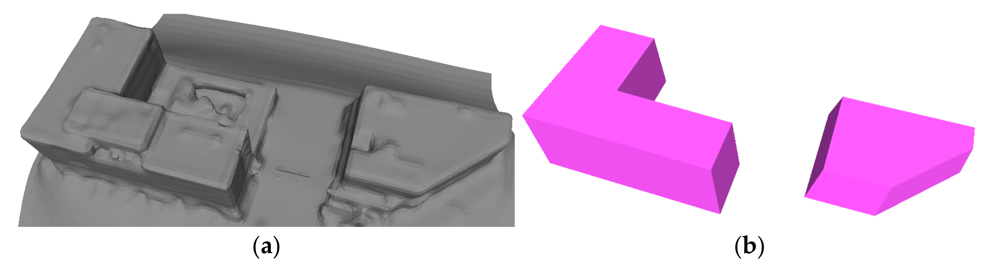
Model (e) and model (f) are the results of Poisson reconstruction of the same region adopting different depth values. Our method achieved a better mesh simplification result without changing parameters. When Poisson reconstruction results of model (d) with smaller depth values are simplified with the same parameters, its main structure can still be reconstructed, as shown in Figure 16, which indicates that our method was less dependent on parameters. However, as the level of detail decreases, fewer building details can be reconstructed with the same threshold.
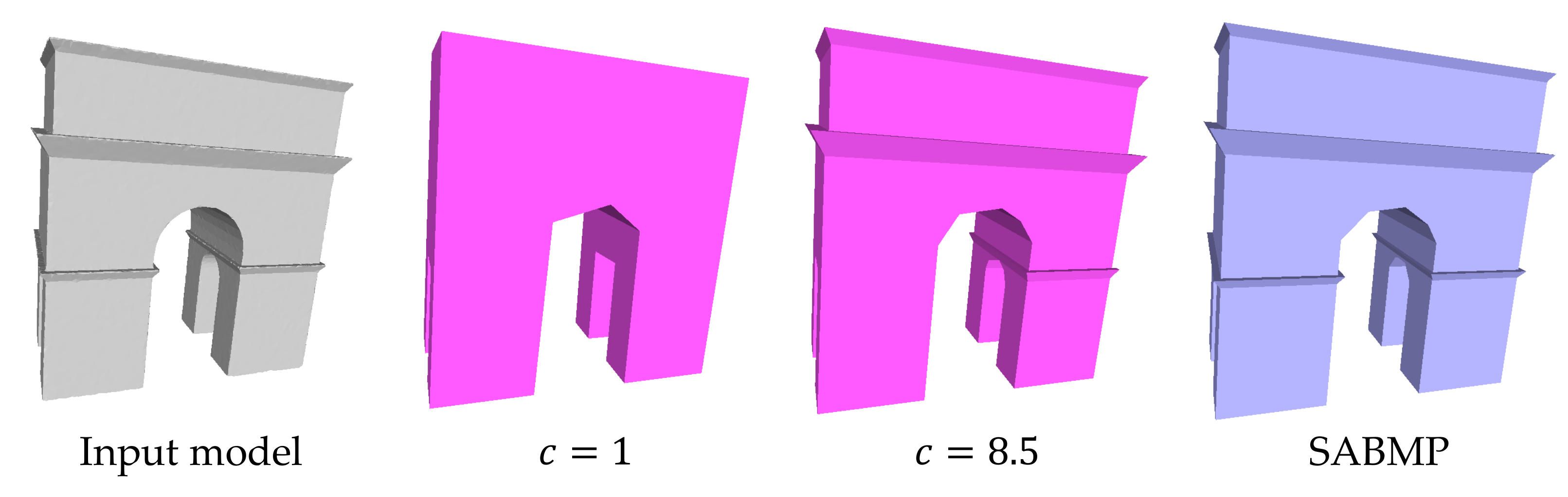
In addition to the degree of fineness, the quality of the mesh model also greatly affected the simplification result. In the case of high model quality, the growing distance threshold can be reduced to improve the degree of refinement. The initial mesh model in Figure 17 has almost no noise, and the simplified model will lose a lot of surface details when using the conventional distance coefficient ( = 1). In the use of a larger distance coefficient, our method could keep most of the surface details, but there was still some detail damage compared to SABMP because the use of the 1-ring patch caused the loss of a small number of trivial planes.
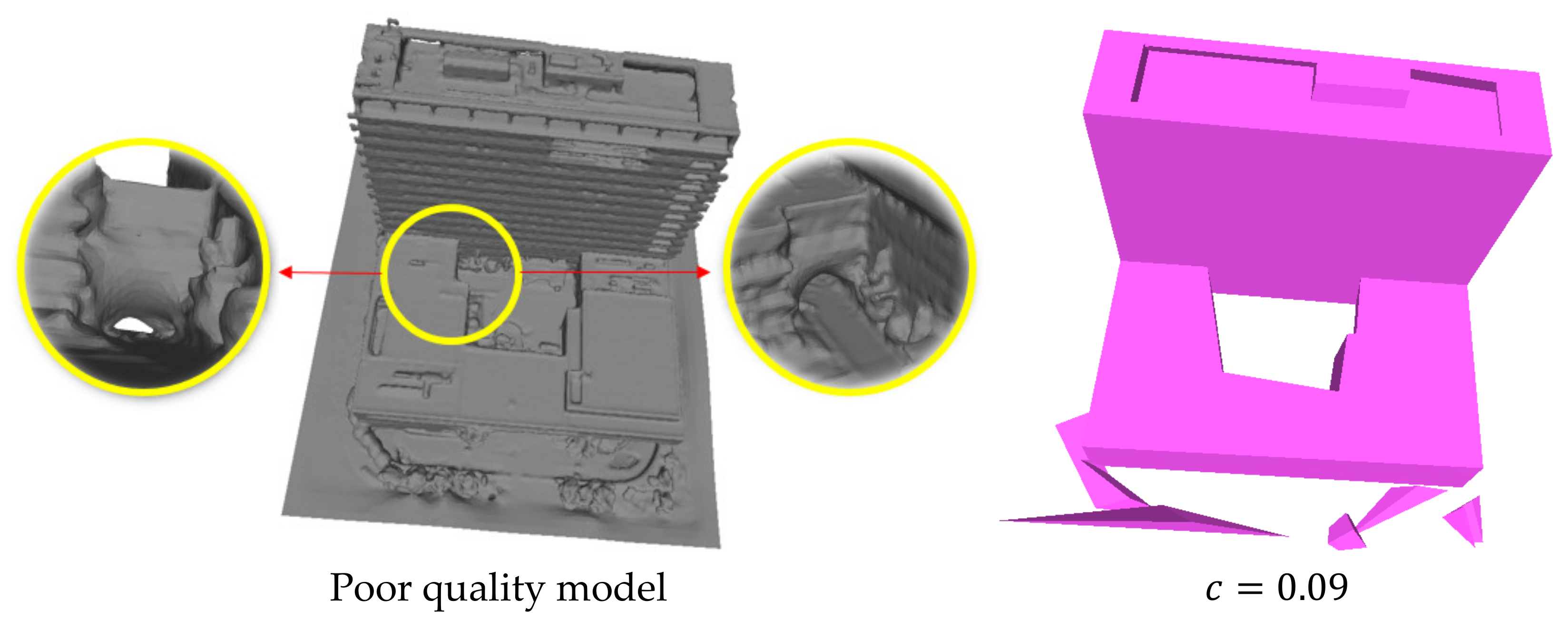
In the case of poor model quality, the threshold of growing distance can be increased to avoid failure of simplification. The initial mesh model in Figure 18 was the result of a more refined Poisson reconstruction result of model (g), however, the increased fineness also amplified the quality issues. The area of the yellow circle in the figure is a narrow and long channel with an irregular curved surface. It is this region that caused the failure of obtaining an ideal simplified model when using the conventional distance coefficient. When the distance coefficient was set to 0.09, the simplification effect was better than that of model (g).
4.2. Non-Monomer Model Optimization Capability
For model (b), SABMP regards it as two independent buildings and simplifies its mesh model into two separate polygonal models. It can be seen that SABMP can deal with non-monomer models. However, the polygonization performance depends on the area coefficient. For the mesh model of a large area, the importance degree determined by the proportion of plane region area to total area is easy to lead to the loss of important structure of the building. In addition, the time consumption of this method increases sharply with the number of meshes and the complexity of the simplified model, so this paper did not carry out non-monomer model reconstruction experiments on it.
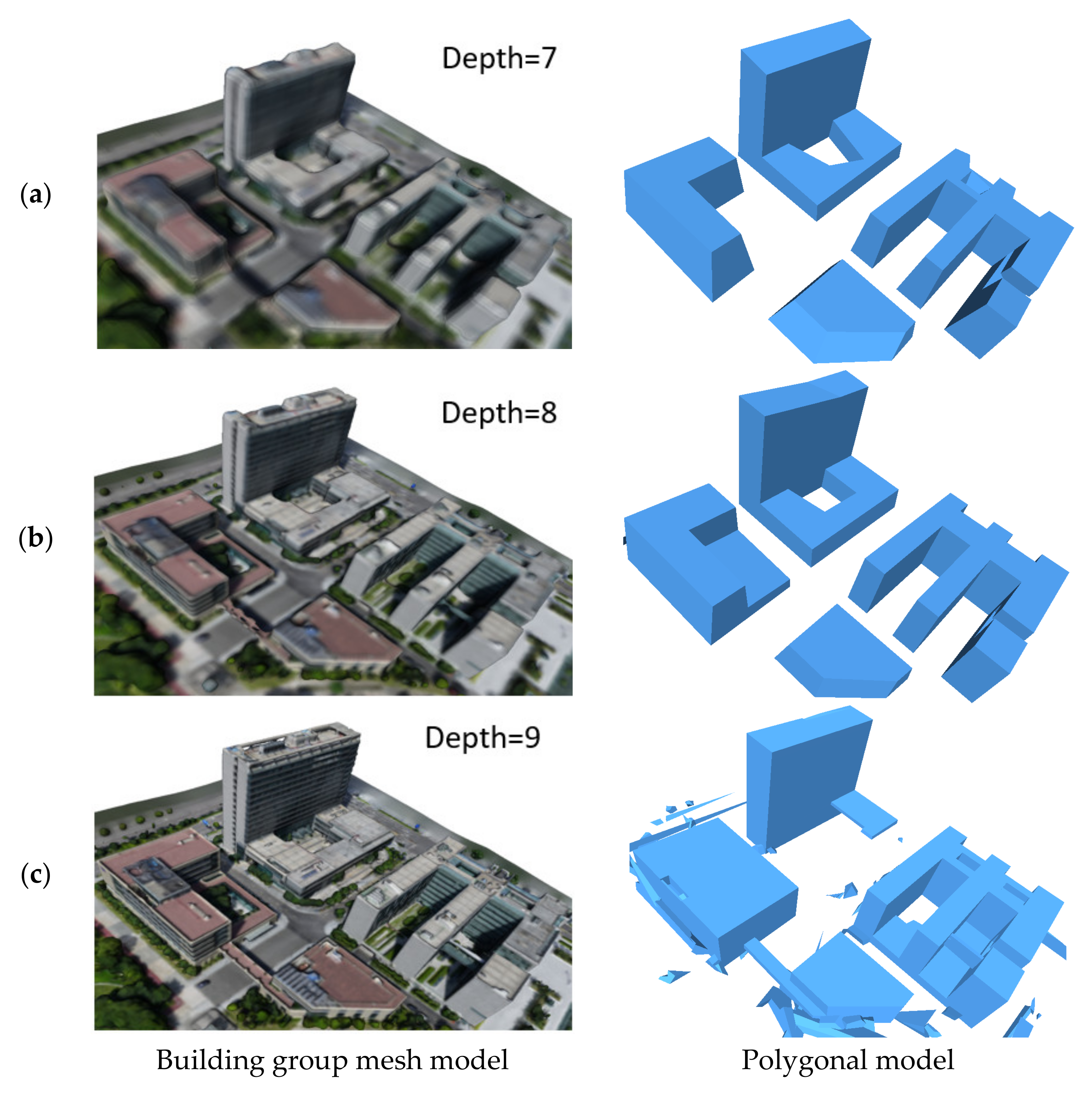
Model (d), model (e), and model (g) are monomer mesh data collected and generated by us in Ningbo, China, and they are adjacent to each other in geographical space. Without building extraction or non-building filtering, our method can still obtain the polygonal model of the whole region derived from the MVS mesh model, as shown in Figure 19.
Some quantitative indexes involved in the experiment are shown in Table 5. The reconstruction results with depth values of 7 and 8 obtained the best modeling results without adjusting the parameters, but the performance could not compare with the result of processing the monomer models separately. For the model with a depth value of 9, the main structure of all buildings could be well restored if the distance coefficient was set as 0.5. The building model to which model (e) belongs achieved better performances than that in Figure 19a,b in retaining important structures. A large number of non-building regions in Figure 19c were not filtered out, which led to too many faces in the final result and a slower mesh conversion rate than other models.
4.3. Limitation
The ideal mesh optimization method, in our mind, could obtain a polygonal model of large-scale building group mesh with arbitrary fineness and mesh quality without adjusting any parameters. The method in this paper relies on the plane extraction and the correct establishment of adjacency relations. Although some wrong adjacency relations have been corrected by using topology optimization, there is still the possibility of failure in the reconstruction of topology relations in some regions with extremely complex structures. To obtain the optimal simplification result, the distance coefficient still needs to be adjusted in some cases, as shown in Figure 17 and Figure 18. As for the control of running time, our work greatly improved the algorithm efficiency without using high-performance computing technologies, such as multi-threading acceleration or GPU acceleration, which make the mesh processing rate nearly constant. However, if the simplified model has too many details, the algorithm efficiency will decrease, as shown in model (f). For the optimization of the building group mesh model, the algorithm in this paper would retain too many non-building features when the mesh was too fine and the non-building region was too complex, as shown in Figure 19c.
5. Conclusions
This paper introduced a simplification strategy of the building surface mesh model based on the 1-ring patch and topology optimization. We improved the strategy of plane extraction, using the 1-ring patch as the primitive, and combined it with triangular facets to perform region growth, which greatly reduced the running time of plane extraction. Aiming at the problems existing in the results of plane extraction, topology optimization was carried out to avoid structural degradation in some important topological regions. In addition, our method improved the topology optimization and polygonal model generation process to greatly improve efficiency. The advantages of strong adaptive parameters and significantly reduced processing time make the method in this paper have considerable practicability and good robustness to the noise of the building surface and adjacent ground. As shown in the experimental results, our methodology outperforms other state of the art mesh polygonization methods in efficiency, structural authenticity, and parameter adaptability. Moreover, with the similar time consummation, our method can obtain a model more sensitive to building structure information than the mesh decimation method. The performance of our method shows great potential in the field of automatic urban buildings reconstruction based on MVS, which is applied in urban management, solar potential estimation, etc.
It should be noted that our current topology optimization strategy cannot fully recover the structure of any type of building model, especially for those with complex curved surface regions. To solve this problem, future extensions of the research will focus on designing the mesh simplification process for the curved region independently. And the processing of oblique image data will be combined to improve the accuracy and precision of the boundaries furtherly.
Author Contributions
Y.L. conceived the framework of the algorithm and wrote the manuscript. H.X. designed and carried out the experiment. L.Y. guided the whole process. All authors have read and agreed to the published version of the manuscript.
Funding
This research was funded by the National Key R&D Program of China, grant number 2020YFD1100200.
Institutional Review Board Statement
Not applicable for studies not involving humans or animals.
Informed Consent Statement
Not applicable for studies not involving humans.
Data Availability Statement
The data presented in this study are available on request from the corresponding author.
Conflicts of Interest
The authors declare no conflict of interest.
References
- Albino, V.; Berardi, U.; Dangelico, R.M. Smart cities: Definitions, dimensions, performance, and initiatives. J. Urban Technol. 2015, 22, 3–21. [Google Scholar] [CrossRef]
- Lehner, H.; Dorffner, L. Digital geoTwin Vienna: Towards a digital Twin City as Geodata Hub; Springer: Cham, Switzerland, 2020. [Google Scholar]
- Nex, F.; Remondino, F. UAV for 3D mapping applications: A review. Appl. Geomat. 2014, 6, 1–15. [Google Scholar] [CrossRef]
- Yao, H.; Qin, R.; Chen, X. Unmanned aerial vehicle for remote sensing applications—A review. Remote Sens. 2019, 11, 1443. [Google Scholar] [CrossRef] [Green Version]
- Stathopoulou, E.K.; Remondino, F. Open-source image-based 3D reconstruction pipelines: Review, comparison and evaluation. In Proceedings of the 6th International Workshop LowCost 3D–Sensors, Algorithms, Applications, Strasbourg, France, 2–3 December 2019. [Google Scholar]
- Aanæs, H.; Jensen, R.R.; Vogiatzis, G.; Tola, E.; Dahl, A.B. Large-scale data for multiple-view stereopsis. Int. J. Comput. Vis. 2016, 120, 153–168. [Google Scholar] [CrossRef] [Green Version]
- Yao, Y.; Luo, Z.; Li, S.; Fang, T.; Quan, L. Mvsnet: Depth inference for unstructured multi-view stereo. In Proceedings of the European Conference on Computer Vision (ECCV), Munich, Germany, 8–14 September 2018. [Google Scholar]
- Schönberger, J.L.; Zheng, E.; Frahm, J.M.; Pollefeys, M. Pixelwise view selection for unstructured multi-view stereo. In European Conference on Computer Vision; Springer: Cham, Switzerland, 2016. [Google Scholar]
- Jia, J.; Huang, M.; Liu, X. Surface reconstruction algorithm based on 3d delaunay triangulation. Acta Geod. Cartogr. Sin. 2018, 47, 281. [Google Scholar]
- Lorensen, W.E.; Cline, H.E. Marching cubes: A high resolution 3D surface construction algorithm. ACM Siggraph Comput. Graph. 1987, 21, 163–169. [Google Scholar] [CrossRef]
- Kazhdan, M.; Hoppe, H. Screened poisson surface reconstruction. ACM Trans. Graph. (ToG) 2013, 32, 1–13. [Google Scholar] [CrossRef] [Green Version]
- MeshLab. Available online: https://www.meshlab.net/ (accessed on 23 October 2021).
- Geomagic Wrap 3D Scanning Software. Available online: https://www.3dsystems.com/software/geomagic-wrap (accessed on 23 October 2021).
- Agisoft Metashape. Available online: https://www.agisoft.com/ (accessed on 23 October 2021).
- VisualSFM: A Visual Structure from Motion System. Available online: http://ccwu.me/vsfm/ (accessed on 23 October 2021).
- Rossignac, J.; Borrel, P. Multi-Resolution 3D Approximations for Rendering Complex Scenes; Modeling in Computer Graphics; Springer: Berlin/Heidelberg, Germany, 1993; pp. 455–465. [Google Scholar]
- Jakob, W.; Tarini, M.; Panozzo, D.; Sorkine-Hornung, O. Instant field-aligned meshes. ACM Trans. Graph. 2015, 34, 181–189. [Google Scholar] [CrossRef]
- Garland, M.; Heckbert, P.S. Surface simplification using quadric error metrics. In Proceedings of the 24th Annual Conference on Computer Graphics and Interactive Techniques, Los Angeles, CA, USA, 3–8 August 1997. [Google Scholar]
- Salinas, D.; Lafarge, F.; Alliez, P. Structure-Aware Mesh Decimation; Wiley Online Library: Hoboken, NJ, USA, 2015. [Google Scholar]
- Li, M.; Nan, L. Feature-preserving 3D mesh simplification for urban buildings. ISPRS J. Photogramm. Remote. Sens. 2021, 173, 135–150. [Google Scholar] [CrossRef]
- Cohen-Steiner, D.; Alliez, P.; Desbrun, M. Variational Shape Approximation; ACM SIGGRAPH 2004 Papers; ACM: New York, NY, USA, 2004; pp. 905–914. [Google Scholar]
- Kelly, T.; Femiani, J.; Wonka, P.; Mitra, N.J. BigSUR: Large-scale structured urban reconstruction. ACM Trans. Graph. 2017, 36, 204. [Google Scholar] [CrossRef]
- Bouzas, V.; Ledoux, H.; Nan, L. Structure-aware Building Mesh Polygonization. ISPRS J. Photogramm. Remote. Sens. 2020, 167, 432–442. [Google Scholar] [CrossRef]
- Sampath, A.; Shan, J. Segmentation and reconstruction of polyhedral building roofs from aerial lidar point clouds. IEEE Trans. Geosci. Remote Sens. 2009, 48, 1554–1567. [Google Scholar] [CrossRef]
- Xu, L.; Kong, D.; Li, X. On-the-fly extraction of polyhedral buildings from airborne LiDAR data. IEEE Geosci. Remote Sens. Lett. 2014, 11, 1946–1950. [Google Scholar]
- Biljecki, F.; Stoter, J.; Ledoux, H.; Zlatanova, S.; Çöltekin, A. Applications of 3D City Models: State of the Art Review. ISPRS Int. J. Geo-Inf. 2015, 4, 2842–2889. [Google Scholar] [CrossRef] [Green Version]
- Furukawa, Y.; Curless, B.; Seitz, S.M.; Szeliski, R. Manhattan-world stereo. In Proceedings of the 009 IEEE Conference on Computer Vision and Pattern Recognition, Miami, FL, USA, 20–25 June 2009. [Google Scholar]
- Nardinocchi, C.; Scaioni, M.; Forlani, G. Building extraction from LIDAR data. In Proceedings of the IEEE/ISPRS Joint Workshop on Remote Sensing and Data Fusion over Urban Areas (Cat. No.01EX482), Rome, Italy, 8–9 November 2001. [Google Scholar]
- Xiong, B.; Elberink, S.O.; Vosselman, G. A graph edit dictionary for correcting errors in roof topology graphs reconstructed from point clouds. ISPRS J. Photogramm. Remote Sens. 2014, 93, 227–242. [Google Scholar] [CrossRef]
- Nan, L.; Wonka, P. Polyfit: Polygonal surface reconstruction from point clouds. In Proceedings of the IEEE International Conference on Computer Vision, Venice, Italy, 22–29 October 2017. [Google Scholar]
- Chen, D.; Wang, R.; Peethambaran, J. Topologically aware building rooftop reconstruction from airborne laser scanning point clouds. IEEE Trans. Geosci. Remote Sens. 2017, 55, 7032–7052. [Google Scholar] [CrossRef]
- Kaiser, A.; Ybanez Zepeda, J.A.; Boubekeur, T. A Survey of Simple Geometric Primitives Detection Methods for Captured 3D Data; Wiley Online Library: Hoboken, NJ, USA, 2019. [Google Scholar]
- Shamir, A. A Survey on Mesh Segmentation Techniques; Wiley Online Library: Hoboken, NJ, USA, 2008. [Google Scholar]
- Rashad, M.; Khamiss, M.; Mousa, M. A review on mesh segmentation techniques. Int. J. Eng. Innov. Technol 2017, 6, 18–26. [Google Scholar] [CrossRef]
- Fang, H.; Lafarge, F.; Desbrun, M. Planar shape detection at structural scales. In Proceedings of the IEEE Conference on Computer Vision and Pattern Recognition, Salt Lake City, UT, USA, 18–22 June 2018. [Google Scholar]
- Gatzke, T.D.; Grimm, C.M. Estimating curvature on triangular meshes. Int. J. Shape Modeling 2006, 12, 1–28. [Google Scholar] [CrossRef] [Green Version]
- Mishra, A.; Pandey, A.; Baghel, A.S. Building detection and extraction techniques: A review. In Proceedings of the 2016 3rd International Conference on Computing for Sustainable Global Development (INDIACom), New Delhi, India, 16–18 March 2016. [Google Scholar]
- Ghanea, M.; Moallem, P.; Momeni, M. Building extraction from high-resolution satellite images in urban areas: Recent methods and strategies against significant challenges. Int. J. Remote Sens. 2016, 37, 5234–5248. [Google Scholar] [CrossRef]
- Dixit, M.; Agarwal, S.; Gupta, P. Building Extraction from Remote Sensing Images: A Survey. In Proceedings of the 2020 2nd International Conference on Advances in Computing, Communication Control and Networking (ICACCCN), Greater Noida, India, 18–19 December 2020. [Google Scholar]
- Guthe, M.; Borodin, P.; Klein, R. Fast and Accurate Hausdorff Distance Calculation between Meshes[J]. 2005. Available online: https://otik.uk.zcu.cz/handle/11025/1446 (accessed on 23 November 2021).
- Boost C++ Libraries. Available online: https://www.boost.org/ (accessed on 23 October 2021).
- The Computational Geometry Algorithms Library. Available online: https://www.cgal.org/ (accessed on 23 October 2021).
Figure 1.
Pipeline. The parts connected by the dotted line show the restoration of a parapet via topology optimization.
Figure 1.
Pipeline. The parts connected by the dotted line show the restoration of a parapet via topology optimization.

Figure 2.
The 1-ring patch model generation process from new seeds generation (a) to new patches generation (b). Patches are distinguished by different colors.
Figure 2.
The 1-ring patch model generation process from new seeds generation (a) to new patches generation (b). Patches are distinguished by different colors.

Figure 3.
The schematic diagram of the k-ring neighborhood and hierarchical index relationship. The orange region is the 1-ring neighborhood of the center point (a) 1-ring, the green region is the expansion of the 2-ring neighborhood compared to the 1-ring neighborhood, and the purple region is the expansion of the 3-ring neighborhood compared to the 2-ring neighborhood. In (b), the 2-ring neighborhood can be covered by six 1-ring neighborhoods (three red boxes and three yellow boxes), and in the same way, the 3-ring neighborhood in (c) can be covered by six 2-ring neighborhoods (only one red box and one yellow box are drawn for aesthetic purposes).

Figure 4.
The input MVS building model (a) expressed by 37,269 triangular facets can be covered with the 1-ring patch model (b) consisting of 4945 patches (each patch is rendered with a random color) and 3496 independent triangular facets (black pieces).
Figure 4.
The input MVS building model (a) expressed by 37,269 triangular facets can be covered with the 1-ring patch model (b) consisting of 4945 patches (each patch is rendered with a random color) and 3496 independent triangular facets (black pieces).

Figure 5.
Two-step strategy of region growth. As shown in the area of the golden ellipse in planar region A and planar region B, in addition to complete patches, the degenerate triangles and independent triangles at the boundary are accurately segmented into the corresponding plane region (different colors represent different plane regions). In general, the scattered black faces that are not labeled as any plane region are too negligible to influence the extraction of the importance of plane region.

Figure 6.
Ground extraction results. (a) is the top view of the result of regional growth, (b) is the result after extracting ground where the ground is highlighted in green, and (c) is the extracted ground region under the oblique and horizontal viewing angles.
Figure 6.
Ground extraction results. (a) is the top view of the result of regional growth, (b) is the result after extracting ground where the ground is highlighted in green, and (c) is the extracted ground region under the oblique and horizontal viewing angles.

Figure 7.
Connection plane rebuilding example. (a) is the top view of the initial segmentation result, and inside the green circle is the parapet formed by the directed connection of two parallel planes; (b) is the side view of (a); (c) is the result of topology modification, the white circle is the horizontal connection plane (corresponding to the pink faces in (d,e)), and the gold circle is the vertical connection plane (corresponding to the blue faces in (d,e)); (d,e) are the close-ups of the parapet of the simplified model in the top and side view, respectively.


Figure 8.
The split of line segments. (a) is the side view of a pair of line segments (labeled in black and gray) to be split. (b) is the top view of the line segments before splitting. After splitting, line segments were divided into four (labeled in different colors), and new corners (purple dot) and candidate faces (labeled in different colors) were formed in (c,e). (d) is the processed scaffold. (e) presents the 3D partitioning result divided by the candidate faces, where the top part is omitted.

Figure 9.
(a–g) Polyhedral results of different building mesh models. From left to right: the original mesh models, the results of VSA [17], the results of SABMP [19], and our results.


Figure 10.
The problem of VSA result. (a), substantial retention of non-architectural details; (b), topology problem. There are two holes in the blue circle and a dangling facet in the red circle.
Figure 10.
The problem of VSA result. (a), substantial retention of non-architectural details; (b), topology problem. There are two holes in the blue circle and a dangling facet in the red circle.

Figure 11.
Example of structure-preserving capabilities. (a) Several parapets (gold circle) are successfully restored; (b) as a result of the restoration of the parapet, the adjacent structure is correctly reconstructed; (c) as a result of the topological modification of the slit region (green circle), the building structure on the left is also correctly restored; (d) connecting corridor (blue circle) is properly rebuilt.


Figure 13.
Accuracy comparison results of SABMP model (a–f). The error of more than 1 m is also shown in red.
Figure 13.
Accuracy comparison results of SABMP model (a–f). The error of more than 1 m is also shown in red.


Figure 14.
Comparison of ground discrimination results. The area of the purple circle should be the ground.
Figure 14.
Comparison of ground discrimination results. The area of the purple circle should be the ground.

Figure 15.
Comparison of running time of different methods.

Figure 16.
Mesh model with a lower fineness (a) and its simplification result (b).

Figure 17.
Simplification effect of the high-quality mesh model.

Figure 18.
Simplification of the poor-quality mesh model. In the area of the yellow circle, there are the regions that are prone to failure of simplification and the enlarged view from different angles.
Figure 18.
Simplification of the poor-quality mesh model. In the area of the yellow circle, there are the regions that are prone to failure of simplification and the enlarged view from different angles.

Figure 19.
Multi-building scene reconstruction results. (a) depth = 7, (b) depth = 8 and, (c) depth = 9.
Figure 19.
Multi-building scene reconstruction results. (a) depth = 7, (b) depth = 8 and, (c) depth = 9.


Table 1.
Comparison of the number of model faces.
| Model | (a) | (b) | (c) | (d) | (e) | (f) | (g) |
|---|---|---|---|---|---|---|---|
| Original | 39,948 | 47,030 | 37,269 | 116,441 | 97,654 | 448,496 | 97,199 |
| VSA | 1567 | 648 | 1322 | 2069 | 1060 | 6840 | 965 |
| Ours | 270 | 198 | 152 | 228 | 246 | 690 | 274 |
| SABMP | 130 | 32 | 100 | 82 | 250 | 344 | 330 |
Table 2.
Comparison of running time of each stage.
| Model | (a) | (b) | (c) | (d) | (e) | (f) | (g) | |
|---|---|---|---|---|---|---|---|---|
| Remodeling (s) | Before optimization | 0.75 | 0.88 | 0.66 | 2.01 | 1.72 | 8.01 | 1.64 |
| SABMP | 0.55 | 0.75 | 0.51 | 1.61 | 1.37 | 6.26 | 1.33 | |
| Ours | 0.38 | 0.39 | 0.32 | 0.92 | 0.77 | 3.84 | 0.76 | |
| Region growing (s) | SABMP | 0.54 | 1.01 | 0.57 | 3.33 | 2.32 | 19.58 | 2.73 |
| Ours | 0.094 | 0.12 | 0.097 | 0.31 | 0.25 | 2.29 | 0.28 | |
| Topological optimization (s) | SABMP | 22.6 | 8.20 | 15.17 | 90.15 | 24.93 | 2435 | 20.62 |
| Ours | 0.053 | 0.096 | 0.052 | 0.23 | 0.15 | 3.18 | 0.18 | |
| Polygonization (s) | Before optimization | 0.44 | 0.17 | 0.17 | 0.65 | 0.36 | 21.63 | 0.27 |
| SABMP | 0.14 | 0.086 | 0.091 | 0.257 | 0.576 | 2.10 | 1.34 | |
| Ours | 0.17 | 0.13 | 0.11 | 0.28 | 0.24 | 2.23 | 0.21 | |
| Total time(s) | SABMP | 23.83 | 10.0 | 16.27 | 95.27 | 29.17 | 2462.7 | 26.53 |
| Ours | 0.697 | 0.736 | 0.579 | 1.74 | 1.41 | 11.54 | 1.43 | |
| Mesh conversion rate | SABMP | 1677 | 4705 | 2291 | 1222 | 3348 | 182 | 3728 |
| Ours | 57,314 | 63,899 | 64,367 | 66,920 | 69,258 | 38,965 | 67,971 | |
Table 3.
Parameter configuration of different models.
| Model | (a) | (b) | (c) | (d) | (e) | (f) | (g) | |
|---|---|---|---|---|---|---|---|---|
| SABMP | Distance coefficient | 1 | 0.9 | 0.9 | 0.8 | 0.6 | 0.6 | 0.5 |
| Area coefficient | 0.2 | 1 | 0.5 | 0.3 | 0.1 | 0.3 | 0.1 | |
| VSA | Agent number | 300 | 100 | 300 | 500 | 300 | 2000 | 300 |
| Ours | 1 | 1 | 1 | 1 | 1 | 1 | 1 | |
Table 4.
The configuration of other parameters.
| Region growing | anglepatch | angletri | / | / | / | / |
| 60° | 40° | / | / | / | / | |
| Topological optimization | disground | hf | anglenonbd | areanonbd | anglemerge | dismerge |
| 4 m | 4 m | 50° | 5 m2 | 5° | 4 |
Table 5.
Some important values of multi-building scene reconstruction.
| Depth | Original Faces | Final Faces | Running Time | Mesh Conversion Rate | |
|---|---|---|---|---|---|
| 7 | 49,982 | 218 | 1 | 0.841 | 59,431 |
| 8 | 214,661 | 380 | 1 | 4.25 | 50,508 |
| 9 | 1,017,002 | 2874 | 0.5 | 72.04 | 14,117 |
Publisher’s Note: MDPI stays neutral with regard to jurisdictional claims in published maps and institutional affiliations. |
© 2021 by the authors. Licensee MDPI, Basel, Switzerland. This article is an open access article distributed under the terms and conditions of the Creative Commons Attribution (CC BY) license (https://creativecommons.org/licenses/by/4.0/).
Share and Cite
MDPI and ACS Style
Yan, L.; Li, Y.; Xie, H. Urban Building Mesh Polygonization Based on 1-Ring Patch and Topology Optimization. Remote Sens. 2021, 13, 4777. https://doi.org/10.3390/rs13234777
AMA Style
Yan L, Li Y, Xie H. Urban Building Mesh Polygonization Based on 1-Ring Patch and Topology Optimization. Remote Sensing. 2021; 13(23):4777. https://doi.org/10.3390/rs13234777
Chicago/Turabian StyleYan, Li, Yao Li, and Hong Xie. 2021. "Urban Building Mesh Polygonization Based on 1-Ring Patch and Topology Optimization" Remote Sensing 13, no. 23: 4777. https://doi.org/10.3390/rs13234777
Note that from the first issue of 2016, this journal uses article numbers instead of page numbers. See further details here.