
Improving the Accuracy of Land Cover Mapping by Distributing Training Samples
by
 ,
,
Chenxi Li
1 ,
,
Zaiying Ma
1,
Liuyue Wang
1,
Weijian Yu
1,
Donglin Tan
1,
Bingbo Gao
1,
Quanlong Feng
1, 
Hao Guo
1 and
Yuanyuan Zhao
1,2,3,* 1
College of Land Science and Technology, China Agricultural University, Beijing 100083, China
2
Key Laboratory of Remote Sensing for Agri-Hazards, Ministry of Agriculture and Rural Affairs, Beijing 100083, China
3
Key Laboratory for Agricultural Land Quality, Ministry of Natural Resources of the People’s Republic of China, Beijing 100083, China
*
Author to whom correspondence should be addressed.
Remote Sens. 2021, 13(22), 4594; https://doi.org/10.3390/rs13224594
Submission received: 25 September 2021
/
Revised: 3 November 2021
/
Accepted: 12 November 2021
/
Published: 15 November 2021
Abstract
:High-quality training samples are essential for accurate land cover classification. Due to the difficulties in collecting a large number of training samples, it is of great significance to collect a high-quality sample dataset with a limited sample size but effective sample distribution. In this paper, we proposed an object-oriented sampling approach by segmenting image blocks expanded from systematically distributed seeds (object-oriented sampling approach) and carried out a rigorous comparison of seven sampling strategies, including random sampling, systematic sampling, stratified sampling (stratified sampling with the strata of land cover classes based on classification product, Latin hypercube sampling, and spatial Latin hypercube sampling), object-oriented sampling, and manual sampling, to explore the impact of training sample distribution on the accuracy of land cover classification when the samples are limited. Five study areas from different climate zones were selected along the China–Mongolia border. Our research identified the proposed object-oriented sampling approach as the first-choice sampling strategy in collecting training samples. This approach improved the diversity and completeness of the training sample set. Stratified sampling with strata defined by the combination of different attributes and stratified sampling with the strata of land cover classes had their limitations, and they performed well in specific situations when we have enough prior knowledge or high-accuracy product. Manual sampling was greatly influenced by the experience of interpreters. All these sampling strategies mentioned above outperformed random sampling and systematic sampling in this study. The results indicate that the sampling strategies of training datasets do have great impacts on the land cover classification accuracies when the sample size is limited. This paper will provide guidance for efficient training sample collection to increase classification accuracies.
1. Introduction
High-quality land cover maps are the basis for monitoring the status and dynamics of the earth’s surface and one of the crucial parameters to understand the processes of a region [1,2]. They have been widely used in land resource management [3], disaster monitoring [4], and environmental assessment [5]. In supervised land cover classification, training samples, classifiers, and auxiliary data are the main factors that affect classification accuracy [6]. A large number of studies have evaluated different classifiers [7,8] and explored the application of various auxiliary data [9,10,11]. The classification accuracy could be improved when they use excellent classifiers and adequate auxiliary data. However, the most direct way to increase classification accuracy is to use sufficient and high-quality training samples [10,12,13,14].
Traditionally, training samples are collected through fieldwork or manual interpretation of high-resolution Google Earth images, which are both time- and labor-consuming. So, collecting training sample sets with a large sample size is tough, especially for large-scale land cover mapping. The representativeness of training samples has a significant impact on the supervised land cover classification [12,15,16]. However, the training samples collected by traditional methods are likely to be biased, which may lead to problems such as an unbalanced spatial distribution of samples and unbalanced sample proportion between classes. For example, manually selected samples are usually distributed in large-scale homogeneous blocks that are easy to reach in the field and easy to identify by visual interpretation. The samples selected in a homogeneous block are usually similar, with strong autocorrelation in the sample set, which often results in poor representativeness [17]. In supervised land cover classification, insufficient and unrepresentative training samples are considered to be the main cause of classification errors [13,15]. Therefore, the training samples need to represent the actual features of the earth’s surface accurately.
At present, a few studies have explored the distribution of samples [18,19,20,21]. In these studies, simple random sampling, stratified sampling, and even distribution among classes were investigated. The conclusions were not consistent, but most studies indicated that when more attention was paid to the overall accuracy, distributing samples according to the proportion to strata and distributing them balanced in regions were helpful to improve the classification accuracy [10,20,21]. To obtain better classification results with fewer but informative labeled samples, active learning was widely used in land cover classification using remotely sensed images [22,23]. People interacted with the classifier continuously, looking for the most informative sample locations to be labeled and significantly reduced the labeling cost [24]. However, most of the samples selected by active learning were located on the boundary of two land cover types, which were mixed pixels. Although the amount of information and uncertainty of these samples were high, they usually did not contribute much to comprehensively representing various land cover types. Previous studies usually compared at most three sample distribution strategies limited to one specific study area. There is no comprehensive evaluation of all common strategies over large areas. Therefore, it is of great significance to develop a reasonable distribution method of training samples suitable for multi regions in land cover classification.
In this paper, we aim at developing a training sample distribution method to improve the representativeness and diversity of samples. Two specific objectives include (1) proposing an object-oriented sampling approach by segmenting image blocks expanded from systematically distributed seeds, and (2) in terms of classification accuracy and sample diversity, quantitatively comparing the proposed method with traditional probability sampling, stratified sampling, and manual sampling.
2. Study Area and Data
2.1. Study Area
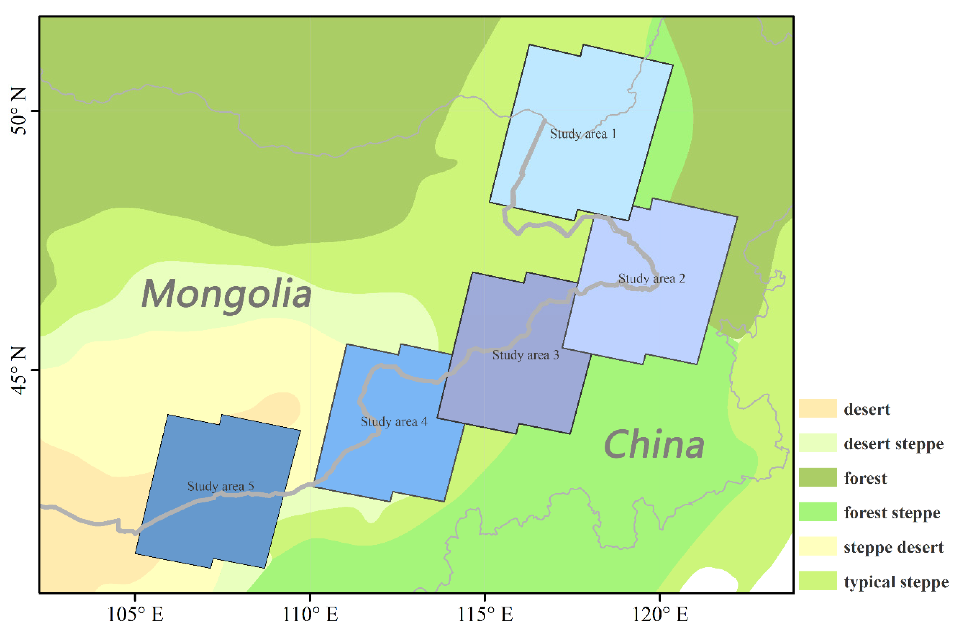
The China–Mongolia–Russia Economic Corridor has become a fast-developing region under the One Belt and One Road Initiative, which calls for accurate land cover maps of high spatial and temporal resolution. Mongolia and Inner Mongolia of China have various types of climate basically along the precipitation gradient from wet (east) to dry (west). The best practice of training sample collection is necessary when producing large-scale land cover maps. We selected five study areas with great differences in climate in the China–Mongolia border to explore the impact of training sample distribution on the accuracy of land cover classification.
To determine the study sites, we partitioned the eco-zones by applying an ISO clustering algorithm to cluster the spatial data layers of elevation, annual average temperature, annual precipitation, coefficient of variation of precipitation, normalized difference vegetation index (NDVI), and the land cover type, and four to 10 clusters were tested to get a better result. The clustering results were compared with the “ecological regionalization map of Inner Mongolia Autonomous Region” [25], and the one with the cluster number of six was chosen due to the highest consistency with the reference data.
The ecological zoning factors used in this paper include elevation, average temperature, precipitation, precipitation variation coefficient, normalized difference vegetation index (NDVI), and land cover type. The source and spatial resolution of data/products are shown in Table 1. Average temperature and Precipitation were monthly climate data, which were first processed into annual average temperature and annual precipitation respectively, and the bioclimatic factor was the precipitation variation coefficient (Bio15). Due to the inconsistent spatial resolution of the data used, the data were unified to 30 s, and then, the data were standardized, fuzzy overlay, and ISO clustering unsupervised classification, and finally, the regional ecological zoning map was obtained. The five study sites were selected basically according to the eco-zones, which are 92,300 square kilometers around Manzhouli, Arshan, Dongwuzhumuqin Banner, Erenhot, and Wulate Rear Banner (Figure 1).
2.2. Data
The remote sensing imagery used in this paper is the Sentinel-2 satellite surface reflectance product (MultiSpectral Instrument, Level-2A) of the European Copernicus satellite program in 2020. Both Sentinel-2 satellites are equipped with MSI multi-spectral sensors, which can provide multi-scale, medium, and high spatial resolution remote sensing images ranging from visible light, near-infrared to shortwave infrared. This series of satellites set four bands in the red edge area of the vegetation spectrum (Band5–Band7, Band8A), so it is effective for monitoring vegetation growth and health. In this paper, Sentinel-2 surface reflectance data in four phases are used for land cover classification. Sentinel-2 band information is shown in Table 2.
3. Methods
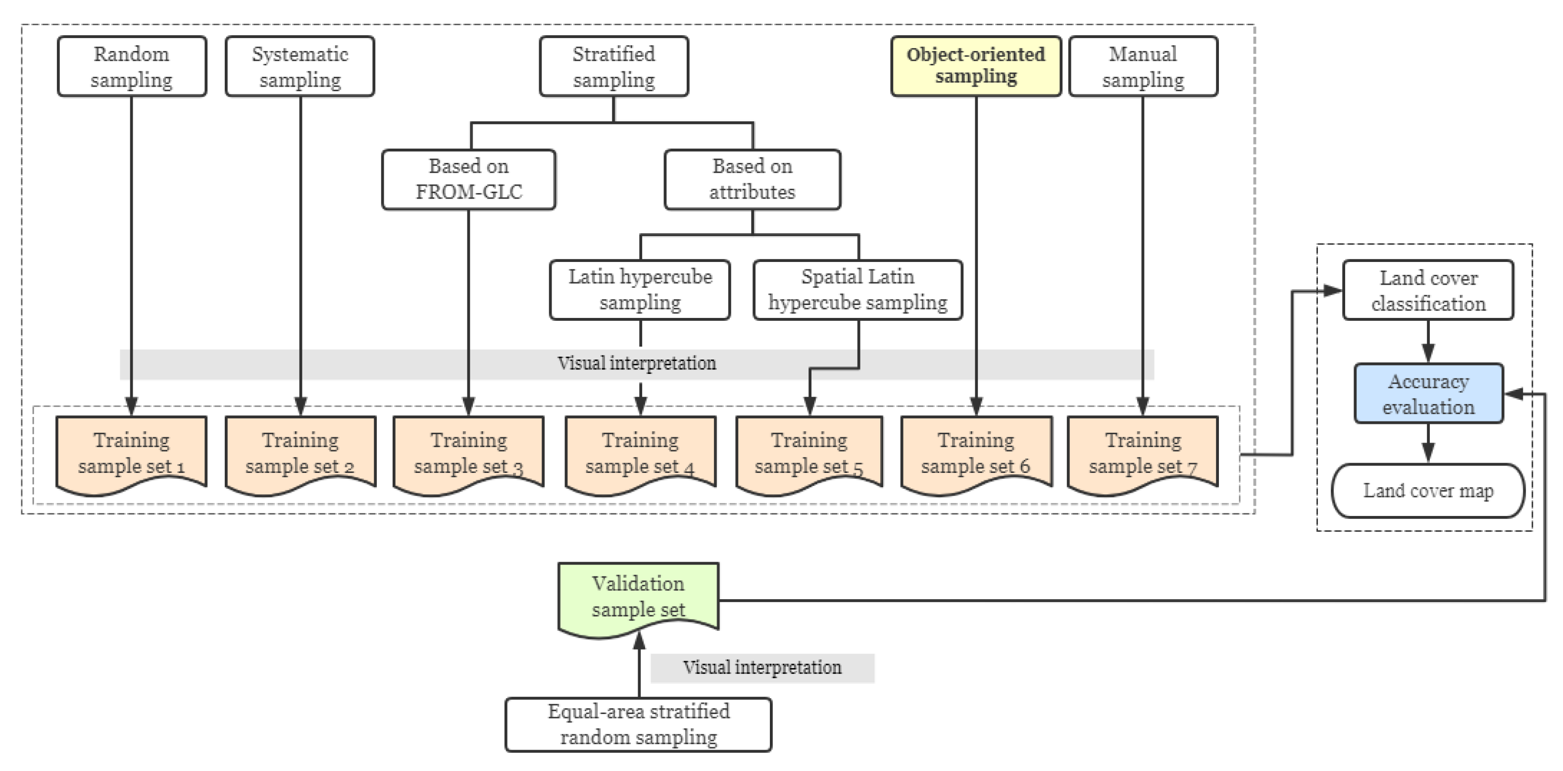
Random sampling, systematic sampling, stratified sampling, object-oriented sampling, and manual sampling were investigated in this study to distribute training samples. In each study area, 200 training sample locations were distributed according to different distribution methods, and then the samples were visually interpreted and the land cover type labels were given. We conduct the experiment on the Google Earth Engine (GEE) platform, which provides a large number of remote sensing data [26]. Using multi-temporal Sentinel-2 surface reflectance data as the basis, the spectral characteristics of four time phases and the NDVI, NDBI, and NDWI spectral index characteristics of four time phases were selected. In each study area, the samples obtained with different distribution methods were used as the training sample set to train models, and the same validation sample set was used to verify the accuracy of each model, to compare the advantages and disadvantages of the training sample distribution methods in each study area. The workflow of this study is shown in Figure 2.
3.1. Classification Scheme
The premise of land cover classification is to design a classification scheme. Based on the FROM-GLC [27] first-level classification scheme and the actual situation of the study area, we designed a land cover classification scheme for the study area (Table 3). This classification scheme can fully describe the land cover in the study area and can be cross-walked better to other land cover classification schemes, such as FAO and IGBP.
3.2. Training Sample Distribution Strategies
We used seven training sample distribution strategies: random sampling, systematic sampling, stratified sampling (stratified sampling with the strata of land cover classes based on classification product, Latin hypercube sampling, and spatial Latin hypercube sampling), object-oriented sampling, and manual sampling. Each strategy distributed 200 training samples.
3.2.1. Traditional Probability Sampling
Simple random sampling (M1) is the most basic sampling method. In this method, each location has an equal chance to be selected from the population as a training sample point. In spatial sampling, it is believed that simple random sampling is suitable for the situation where the spatial sample is uniformly distributed and the spatial variation is stable [28]. In this paper, based on the 5 study areas, random sampling was carried out in each study area to distribute the training sample points.
Systematic sampling (M2) is also called mechanical sampling or equidistant sampling. First, the units in the population are arranged in a certain order, and the sampling interval is determined according to the needs of the sample size; then, the starting point is randomly determined, and a sample unit is drawn at regular intervals. In this paper, based on the external rectangles of 5 study areas, systematic sampling was carried out according to equal spacing, and then the sample locations were selected.
3.2.2. Stratified Sampling
Stratified sampling is to divide a population unit into several types or strata according to its attribute characteristics and then randomly select samples from the types or strata. Through stratification, the samples in each stratum have a certain commonality. The core of the stratified sampling method is to obtain the sample with the highest sampling efficiency. It is generally believed that stratified sampling makes it easy to extract representative samples [29]. In this paper, we considered stratified sampling with area proportion and stratified sampling with a combination of attributes.
Stratified sampling with the strata of land cover classes based on classification product (M3): This paper was based on the FROM-GLC with 10 m resolution in 2017 (downloaded from http://data.ess.tsinghua.edu.cn/, accessed on 10 May 2021). A total of 200 sample points were selected from all land cover types in each study area.
Stratified sampling with strata defined by the combination of different attributes, including climate and topographic variables: elevation, annual average temperature, annual precipitation, coefficient of variation of precipitation, and land cover type are considered for stratified sampling in each study area. The sampling methods used include Latin Hypercube sampling (M4) and spatial Latin hypercube sampling (M5). Spatial Latin hypercube sampling can ensure a more even distribution of samples in space.
3.2.3. Object-Oriented Sampling by Segmenting Image Blocks Expanded from Systematically Distributed Seeds (Object-Oriented Sampling)
We proposed an object-oriented sampling approach (M6). The simple workflow of the object-oriented sampling approach is shown in Figure 3. To ensure that the size of each sample set is the same, the systematic samples were sampled at intervals and extracted 40 samples as seeds. Then, we took the seeds as the center and expanded blocks with a side length of 1–10 km outwards. The average, median, and mode of land cover types included in the FROM-GLC in the blocks of each side length were counted, and the block with mode 3 was selected as the extension range. Then, based on the multi-temporal spectral features and spectral index features, unsupervised clustering was performed in each block, and the number of clusters was 5. In each block, based on the clustering results, five sample locations representing five objects were randomly selected for visual interpretation. Finally, the random samples in all blocks were taken as the training samples to form the training sample set of object-oriented sampling.
3.2.4. Manual Sampling
The image analyst chose 200 sample locations manually in each study area and labeled them on the platform of GEE (M7). Among the manually selected training samples, the sample size of various land cover types is relatively balanced.
3.3. Visual Interpretation
We trained the interpreters before interpreting. The background knowledge of climate and topography in the study area, Google Earth’s very-high-resolution (VHR) images, the reflectance spectrum curve, and the time series NDVI curve extracted from GEE are the reference information for labeling. VHR satellite imagery is an important reference for visual interpretation [30,31,32]. According to the above information, interpreters gave an integrated label of the sample location’s land cover in a year. The integrated label was given based on “the greenest” principle and “the wettest” principle, and “the greenest” took precedence over “the wettest”; that was, the vegetation category had the highest priority when determining the integrated land cover type [33]. One interpreter labeled all samples distributed by M1 to M6 in a study area. Through random inspection, the labels given by the interpreters were credible.
3.4. Classification
There are many types of feature variables used in land cover classification, including spectral, temporal, and geological auxiliary features. Spectral features are one of the most commonly used features [34,35]. Multi-temporal features have advantages in obtaining seasonal changes in the spectrum of ground features, and they can determine the land cover type based on the changing characteristics [33,36,37]. The NDVI (Equation (1)), NDBI (Equation (2)), and NDWI (Equation (3)) spectral index characteristics were sensitive to vegetation, built-up areas, and water bodies, respectively. The most commonly used auxiliary features are topographic features [35,38,39]. Since the five study areas in this paper are small and the topography of the study area is consistent, we did not consider topographic features. Finally, we selected 60 features of the spectrum and spectral index of 4 phases for supervised land cover classification.
3.5. Diversity Evaluation
Training samples in land cover classification need to be accurate and comprehensively represent various land cover types. So, the samples need to be diverse. We believe that the diversity of training sample sets collected by various methods may be different. We calculated the Euclidean distance (Equation (4)) and variance (Equation (5)) between samples in each training sample set based on multi-temporal characteristics and used the variance to represent the diversity. In Equation (4), m is the dimensions of the feature vector of samples. The xk and yk represent the feature vector samples. d is the Euclidean distance between two multi-dimensional vectors. We calculated the Euclidean distance between every two samples in every sample set. Then, the variance of Euclidean distance of each sample set was calculated to represent the diversity. In Equation (5), n represents the sample size, and di and represent the Euclidean distance and the average of the distance, respectively.
3.6. Accuracy Assessment
In each study area, we used an accurate validation sample set that was independent of the training sample sets to evaluate classification accuracy. Validation samples were distributed by equal-area stratified random sampling [42], which ensured that the validation samples were uniformly distributed in the global and randomly distributed in the local.
We compared the advantages and disadvantages of each distribution method through overall accuracy (OA), F1 score, confusion matrix, sample diversity, and classification maps.
4. Results
4.1. Sample Diversity
Table 4 shows the diversity of the sample set (S1–S7) collected by each sampling method (M1–M7) in each study area.
From Table 4, we found that the sample diversity of M6 is among the top for all study areas. For study areas 3 and 4, the sample diversity of M5 is richest, but M6 is close to M5. Therefore, the training samples collected by the proposed object-oriented sampling approach have rich diversity. Overall, the sample sets in study area 2 and study area 5 have the richest and worst diversity, respectively. That is because there are differences in land cover between the two study areas. Study area 2 is located in the forest-steppe ecological area and forest ecological area. The land cover types in this study area are diverse, and it is easy to collect various samples. So, the diversity of training samples collected by each method in study area 2 is richer than that in other study areas. Study area 5 is located in the desert ecological area, and two main types are grassland and barren land. Due to the dry climate, these two types are similar and difficult to distinguish. So, the diversity metrics of training samples collected by all methods in study area 5 are low.
4.2. Classification Accuracy
Due to the subjectivity of manual sampling (M7), its performance varied greatly in the different study areas, so it was not objectively compared with other methods. The differences of sampling methods in each study area are statistically significant. The p-value of each study area is less than 0.05.
We compared the two classifiers of RF and support vector machine (SVM) in study area 1. The results show that the OA and F1 scores of RF are 10.24% and 0.0509 higher than those of SVM on average, respectively. Therefore, the results presented in this section are based on RF.
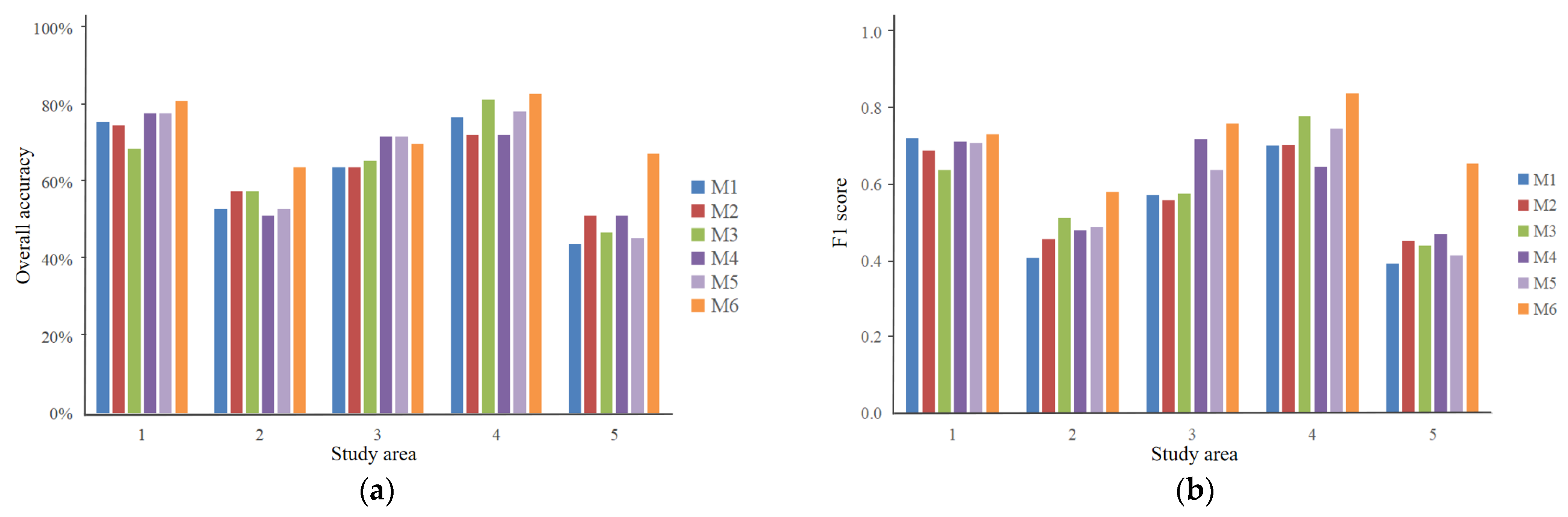
Overall, the classification models built using the training sample sets collected by the object-oriented sampling approach are high-accuracy (Figure 4). We conducted three groups of sampling experiments in study area 1. In each group, the OA and F1 scores of the object-oriented sampling approach are the highest, and the sample diversity is among the top. The results of other study areas are similar to those of study area 1. The accuracy of the stratified sampling with strata defined by the combination of different attributes was high, but it was low in study area 2. The performances of stratified sampling with the strata of land cover classes based on classification product were different in each study area. Random sampling and systematic sampling were not suitable to distribute the training sample locations of land cover.
Figure 5 shows the classification maps based on samples collected by the object-oriented sampling approach and the detailed maps based on each sampling method. We found that the detail maps based on the training samples collected by the object-oriented sampling approach are more accurate. For instance, in study area 2, expect the object-oriented sampling approach; other sampling methods caused the over-classification of forests. In study area 4, the object-oriented sampling approach collected impervious surface samples and water samples, so it identified impervious surface and water effectively. In study area 3, the model built using the training sample sets collected by the object-oriented sampling approach misclassified barren land as impervious surfaces, but it was still the most effective method compared with other methods.
5. Discussions
5.1. Advantages and Disadvantages of Each Sampling Method
The preferred alternative of sample distribution is an object-oriented sampling approach. The object-oriented sampling approach improved the diversity and representativeness of the training sample set, which is helpful for supervised land cover classification. Due to the influence of moisture and topography, the phenology stage and growth state of the vegetation in the study area were different. Therefore, in the blocks with multiple land cover types, we exhausted samples of all land cover classes; that is, the diversity of samples was richer. In the blocks with less land cover types, the randomly selected samples could belong to the same land cover type with different spectral characteristics, such as grassland samples in different growing conditions. Therefore, the spectral representativeness of samples was increased. The object-oriented sampling approach is greatly affected by the size of the blocks and the land cover types within the blocks. The size of blocks can be smaller in areas with strong heterogeneity and larger in areas with strong homogeneity to ensure rich land cover types in image blocks. If there are more land cover types in the systematically distributed image blocks, the training samples will be more diverse and representative. The object-oriented sampling approach performed well in the temperate areas we selected. However, for other temperature zones, such as the tropics, the testing of this approach is not enough. The applicability of this approach in different temperature zones needs to be further tested.
The second option could be stratified sampling with strata defined by the combination of different attribute layers of the study area except for in study area 2, where this method was not suitable. Stratified sampling is affected by the spatial correlation characteristics of geographical objects and the richness of prior knowledge [43]. However, we only combined five attribute layers, and there was a lack of prior knowledge of soil type, socio-economic factors, and so on. Study area 2 was located in the forest-steppe ecological area, with rich land cover types and strong spatial autocorrelation, so the classification model trained with samples collected by this method was not good. Generally, spatial Latin hypercube sampling ensures the balanced distribution of samples spatially. In this study, the difference between the Latin hypercube and the spatial Latin hypercube was not obvious. That may be due to the small spatial range of the five study areas, and the unevenly spatial distribution of the samples had little impact on land cover classification.
Stratified sampling using land cover classes as the strata is one of the most simplified forms based on only one type of prior knowledge. According to the FROM-GLC maps, sample points were obtained from various types proportionally and then labeled with true land cover classes by image analysts. Through visual interpretation, we found that this method was greatly influenced by the time of reference land cover product and its accuracy. When the FROM-GLC is accurate, and the land cover types have not changed, the representativeness of the training sample set can be guaranteed. However, this method has some limitations. For example, some sample points were selected from the strata of forest and water according to the maps of FROM-GLC, and then, the forests were cut down and the water bodies dried up. That will lead to the reduction of the forest and water samples than we expect. For the land cover class with a smaller area and a higher classification error, such as impervious surfaces, the sample points of this land cover class could be missing in the sample dataset. Therefore, this method is greatly affected by the time of the reference product and its accuracy. When using this method to distribute training samples, these two factors should be considered.
Random sampling and systematic sampling are traditional probability sampling methods. These methods assume that the samples are completely independent. However, the land cover types in the region are affected by natural and socio-economic conditions, and they are not completely independent and random. Therefore, traditional sampling methods are limited to distribute land cover training samples.
5.2. Influence of Sample Quality and Sample Size
High-quality training samples are essential for accurate land cover classification. The labels given by the interpreters in this study were highly reliable. However, there is still uncertainty in the image interpretation, especially for some difficult-to-interpret sample points. In study area 5, it was difficult to distinguish between grasslands and barren lands through image interpretation. Therefore, the accuracies of all methods in study area 5 were low.
The number of training samples is another important factor affecting the accuracy of land cover classification. In this paper, we got acceptable accuracy by using 200 samples (S6) based on object-oriented sampling. Then, we used all objective samples (S1–S6, a total of 1200 samples) from each study area to train the classification model. We found that in study areas 1 to 5, the overall accuracy was 4.69%, 3.13%, 3.44%, 10.17%, and 4.41% higher than that using S6 only. Therefore, increasing the number of training samples will improve the accuracy of land cover classification. However, except for study area 4, we used six times the sample size to improve the accuracy by approximately 4%. Thus, the proposed object-oriented sampling approach can obtain acceptable classification accuracy when collecting a small number of samples.
6. Conclusions and Perspectives
We focused on the spatial distribution of training samples of land cover and proposed an object-oriented sampling approach by segmenting image blocks expanded from systematically distributed seeds (object-oriented sampling approach). To explore the impact of sample distribution on classification accuracy, we tested seven sample distribution methods, including random sampling, systematic sampling, stratified sampling (stratified sampling with the strata of land cover classes based on classification product, Latin hypercube sampling, and spatial Latin hypercube sampling), object-oriented sampling, and manual sampling.
We conclude that the object-oriented sampling approach is a good choice for training sample distribution in study areas of different climate types. This sampling approach conducts unsupervised clustering based on multi-temporal spectral bands and spectral indices in each block, and then, the sample locations representing objects were randomly selected. The models trained using the sample set distributed by this method have almost the highest sample diversity and classification accuracy. So, we recommend this approach when distributing training samples for land cover classification.
When the spatial correlation is strong and the attributes data of the study area are rich enough, stratified sampling with strata defined by the combination of different attributes of the study area is the second choice for distributing training samples. Stratified sampling with the strata of land cover classes based on the reference land cover product is greatly affected by the timeliness and accuracy of the reference map. When you have an accurate and latest reference map, this sampling method can get a complete training sample set, and it also a good choice. Since the spatial distribution of land cover is not completely random and independent, random sampling and systematic sampling are weak in distributing a high-quality training sample set.
In addition to the sample distribution method, the quality and quantity of training samples are also important factors influencing land cover classification. Ensuring the quality and increasing the training sample size can improve the classification accuracy. In the future, the optimal combination of sample size and the training sample distribution method will be explored further and tested on datasets in different temperature zones or ecological regions, so as to provide references for the selection of training samples.
Author Contributions
Conceptualization, C.L. and Y.Z.; Data curation, L.W., W.Y. and D.T.; Formal analysis, C.L.; Funding acquisition, Y.Z.; Methodology, C.L. and Z.M.; Resources, L.W., W.Y., D.T., B.G., Q.F. and H.G.; Supervision, Y.Z.; Validation, C.L., Z.M. and Y.Z.; Visualization, C.L.; Writing—original draft, C.L.; Writing—review and editing, Y.Z. All authors have read and agreed to the published version of the manuscript.
Funding
This research was funded by the National Key Research and Development Program of China [grant number 2018YFE0122700], National Natural Science Foundation of China [grant number 42001352]. The APC was funded by the National Key Research and Development Program of China [grant number 2018YFE0122700].
Conflicts of Interest
The authors declare no conflict of interest.
References
- Baudoux, L.; Inglada, J.; Mallet, C. Toward a yearly country-scale CORINE land-cover map without using images: A map translation approach. Remote Sens. 2021, 13, 1060. [Google Scholar] [CrossRef]
- Das, N.; Mondal, P.; Sutradhar, S.; Ghosh, R. Assessment of variation of land use/land cover and its impact on land surface temperature of Asansol subdivision. Egypt. J. Remote Sens. Space Sci. 2021, 24, 131–149. [Google Scholar] [CrossRef]
- Ngo, K.D.; Lechner, A.M.; Vu, T.T. Land cover mapping of the Mekong Delta to support natural resource management with multi-temporal Sentinel-1A synthetic aperture radar imagery. Remote Sens. Appl. Soc. Environ. 2020, 17, 100272. [Google Scholar] [CrossRef]
- Panteras, G.; Cervone, G. Enhancing the temporal resolution of satellite-based flood extent generation using crowdsourced data for disaster monitoring. Int. J. Remote Sens. 2018, 39, 1459–1474. [Google Scholar] [CrossRef]
- Chen, C.Y.; Chen, H.W.; Sun, C.T.; Chuang, Y.H.; Nguyen, K.L.P.; Lin, Y.T. Impact assessment of river dust on regional air quality through integrated remote sensing and air quality modeling. Sci. Total Environ. 2021, 755, 142621. [Google Scholar] [CrossRef]
- Zhao, H.; Wang, J. Research on the factors affecting the classification accuracy of ETM remote sensing image land cover/use. Remote Sens. Tech. Appl. 2012, 27, 600–608. [Google Scholar]
- Priyadarshini, K.N.; Kumar, M.; Rahaman, S.A.; Nitheshnirmal, S. A Comparative Study of Advanced Land Use/Land Cover Classification Algorithms Using Sentinel-2 Data. Int. Arch. Photogramm. Remote Sens. Spat. Inf. Sci. 2018, XLII–5, 665–670. [Google Scholar] [CrossRef] [Green Version]
- Talukdar, S.; Singha, P.; Mahato, S.; Pal, S.; Liou, Y.A.; Rahman, A. Land-use land-cover classification by machine learning classifiers for satellite observations—A review. Remote Sens. 2020, 12, 1135. [Google Scholar] [CrossRef] [Green Version]
- Jia, K.; Liang, S.; Wei, X.; Yao, Y.; Su, Y.; Jiang, B.; Wang, X. Land cover classification of landsat data with phenological features extracted from time series MODIS NDVI data. Remote Sens. 2014, 6, 11518–11532. [Google Scholar] [CrossRef] [Green Version]
- Zhu, Z.; Gallant, A.L.; Woodcock, C.E.; Pengra, B.; Olofsson, P.; Loveland, T.R.; Jin, S.; Dahal, D.; Yang, L.; Auch, R.F. Optimizing selection of training and auxiliary data for operational land cover classification for the LCMAP initiative. ISPRS J. Photogramm. Remote Sens. 2016, 122, 206–221. [Google Scholar] [CrossRef] [Green Version]
- Pflugmacher, D.; Rabe, A.; Peters, M.; Hostert, P. Mapping pan-European land cover using Landsat spectral-temporal metrics and the European LUCAS survey. Remote Sens. Environ. 2019, 221, 583–595. [Google Scholar] [CrossRef]
- Foody, G.M.; Arora, M.K. An evaluation of some factors affecting the accuracy of classification by an artificial neural network. Int. J. Remote Sens. 1997, 18, 799–810. [Google Scholar] [CrossRef]
- Li, C.; Wang, J.; Wang, L.; Hu, L.; Gong, P. Comparison of classification algorithms and training sample sizes in urban land classification with landsat thematic mapper imagery. Remote Sens. 2014, 6, 964–983. [Google Scholar] [CrossRef] [Green Version]
- Persello, C.; Bruzzone, L. Active and semisupervised learning for the classification of remote sensing images. IEEE Trans. Geosci. Remote Sens. 2014, 52, 6937–6956. [Google Scholar] [CrossRef]
- Ghorbanian, A.; Kakooei, M.; Amani, M.; Mahdavi, S.; Mohammadzadeh, A.; Hasanlou, M. Improved land cover map of Iran using Sentinel imagery within Google Earth Engine and a novel automatic workflow for land cover classification using migrated training samples. ISPRS J. Photogramm. Remote Sens. 2020, 167, 276–288. [Google Scholar] [CrossRef]
- Huang, H.; Wang, J.; Liu, C.; Liang, L.; Li, C.; Gong, P. The migration of training samples towards dynamic global land cover mapping. ISPRS J. Photogramm. Remote Sens. 2020, 161, 27–36. [Google Scholar] [CrossRef]
- Mountrakis, G.; Xi, B. Assessing reference dataset representativeness through confidence metrics based on information density. ISPRS J. Photogramm. Remote Sens. 2013, 78, 129–147. [Google Scholar] [CrossRef]
- Ateishi, R.T.; Yush, J.T.S.; Har, M.A.G.; Ilbisi, H.A.L.; Katani, T.O. Sampling Methods for Validation of Large Area Land Cover Mapping. J. Remote Sens. Soc. Japan 2007, 27, 195–204. [Google Scholar] [CrossRef]
- Colditz, R.R. An evaluation of different training sample allocation schemes for discrete and continuous land cover classification using decision tree-based algorithms. Remote Sens. 2015, 7, 9655–9681. [Google Scholar] [CrossRef] [Green Version]
- Jin, H.; Stehman, S.V.; Mountrakis, G. Assessing the impact of training sample selection on accuracy of an urban classification: A case study in Denver, Colorado. Int. J. Remote Sens. 2014, 35, 2067–2081. [Google Scholar] [CrossRef]
- Pagliarella, M.C.; Corona, P.; Fattorini, L. Spatially-balanced sampling versus unbalanced stratified sampling for assessing forest change: Evidences in favour of spatial balance. Environ. Ecol. Stat. 2018, 25, 111–123. [Google Scholar] [CrossRef]
- Lu, Q.; Ma, Y.; Xia, G.S. Active learning for training sample selection in remote sensing image classification using spatial information. Remote Sens. Lett. 2017, 8, 1210–1219. [Google Scholar] [CrossRef]
- Tuia, D.; Ratle, F.; Pacifici, F.; Kanevski, M.F.; Emery, W.J. Active learning methods for remote sensing image classification. IEEE Trans. Geosci. Remote Sens. 2009, 47, 2218–2232. [Google Scholar] [CrossRef]
- Settles, B. Active Learning Literature Survey. Mach. Learn. 2010, 15, 201–221. [Google Scholar]
- Li, B.; Yong, S.; Zeng, S. The principle, method, and application of ecological regionalization—Explanation of the ecological regionalization map of the Inner Mongolia Autonomous Region. Chinese J. Plant Ecol. 1990, 14, 55–62. [Google Scholar]
- Amani, M.; Ghorbanian, A.; Ahmadi, S.A.; Kakooei, M.; Moghimi, A.; Mirmazloumi, S.M.; Moghaddam, S.H.A.; Mahdavi, S.; Ghahremanloo, M.; Parsian, S.; et al. Google Earth Engine Cloud Computing Platform for Remote Sensing Big Data Applications: A Comprehensive Review. IEEE J. Sel. Top. Appl. Earth Obs. Remote Sens. 2020, 13, 5326–5350. [Google Scholar] [CrossRef]
- Gong, P.; Wang, J.; Yu, L.; Zhao, Y.; Zhao, Y.; Liang, L.; Niu, Z.; Huang, X.; Fu, H.; Liu, S.; et al. Finer resolution observation and monitoring of global land cover: First mapping results with Landsat TM and ETM+ data. Int. J. Remote Sens. 2013, 34, 2607–2654. [Google Scholar] [CrossRef] [Green Version]
- Li, L.; Wang, J. Spatial sampling model for geographic data. Prog. Nat. Sci. 2002, 12, 99–102. [Google Scholar]
- Wang, J.F.; Stein, A.; Gao, B.B.; Ge, Y. A review of spatial sampling. Spat. Stat. 2012, 2, 1–14. [Google Scholar] [CrossRef]
- Lesiv, M.; See, L.; Bayas, J.C.L.; Sturn, T.; Schepaschenko, D.; Karner, M.; Moorthy, I.; McCallum, I.; Fritz, S. Characterizing the spatial and temporal availability of very high resolution satellite imagery in Google Earth and Microsoft Bing Maps as a source of reference data. Land 2018, 7, 118. [Google Scholar] [CrossRef] [Green Version]
- Schepaschenko, D.; See, L.; Lesiv, M.; Bastin, J.F.; Mollicone, D.; Tsendbazar, N.E.; Bastin, L.; McCallum, I.; Laso Bayas, J.C.; Baklanov, A.; et al. Recent Advances in Forest Observation with Visual Interpretation of Very High-Resolution Imagery. Surv. Geophys. 2019, 40, 839–862. [Google Scholar] [CrossRef] [Green Version]
- Zhao, Y.; Feng, D.; Jayaraman, D.; Belay, D.; Sebrala, H.; Ngugi, J.; Maina, E.; Akombo, R.; Otuoma, J.; Mutyaba, J.; et al. Bamboo mapping of Ethiopia, Kenya and Uganda for the year 2016 using multi-temporal Landsat imagery. Int. J. Appl. Earth Obs. Geoinf. 2018, 66, 116–125. [Google Scholar] [CrossRef]
- Zhao, Y.; Feng, D.; Yu, L.; Wang, X.; Chen, Y.; Bai, Y.; Hernández, H.J.; Galleguillos, M.; Estades, C.; Biging, G.S.; et al. Detailed dynamic land cover mapping of Chile: Accuracy improvement by integrating multi-temporal data. Remote Sens. Environ. 2016, 183, 170–185. [Google Scholar] [CrossRef]
- Lu, D.; Weng, Q. A survey of image classification methods and techniques for improving classification performance. Int. J. Remote Sens. 2007, 28, 823–870. [Google Scholar] [CrossRef]
- Yu, X.; Lu, D.; Jiang, X.; Li, G.; Chen, Y.; Li, D.; Chen, E. Examining the roles of spectral, spatial, and topographic features in improving land-cover and forest classifications in a subtropical region. Remote Sens. 2020, 12, 2907. [Google Scholar] [CrossRef]
- Rujoiu-Mare, M.R.; Olariu, B.; Mihai, B.A.; Nistor, C.; Săvulescu, I. Land cover classification in Romanian Carpathians and Subcarpathians using multi-date Sentinel-2 remote sensing imagery. Eur. J. Remote Sens. 2017, 50, 496–508. [Google Scholar] [CrossRef] [Green Version]
- Zhao, Y.; Feng, D.; Yu, L.; Cheng, Y.; Zhang, M.; Liu, X.; Xu, Y.; Fang, L.; Zhu, Z.; Gong, P. Long-term land cover dynamics (1986–2016) of Northeast China derived from a multi-temporal landsat archive. Remote Sens. 2019, 11, 599. [Google Scholar] [CrossRef] [Green Version]
- Chen, B.; Huang, B.; Xu, B. Multi-source remotely sensed data fusion for improving land cover classification. ISPRS J. Photogramm. Remote Sens. 2017, 124, 27–39. [Google Scholar] [CrossRef]
- Hurskainen, P.; Adhikari, H.; Siljander, M.; Pellikka, P.K.E.; Hemp, A. Auxiliary datasets improve accuracy of object-based land use/land cover classification in heterogeneous savanna landscapes. Remote Sens. Environ. 2019, 233, 111354. [Google Scholar] [CrossRef]
- Breiman, L. Random Forest. Mach. Learn. 2001, 45, 5–32. [Google Scholar] [CrossRef] [Green Version]
- Gislason, P.O.; Benediktsson, J.A.; Sveinsson, J.R. Random forests for land cover classification. Pattern Recognit. Lett. 2006, 27, 294–300. [Google Scholar] [CrossRef]
- Zhao, Y.; Gong, P.; Yu, L.; Hu, L.; Li, X.; Li, C.; Zhang, H.; Zheng, Y.; Wang, J.; Zhao, Y.; et al. Towards a common validation sample set for global land-cover mapping. Int. J. Remote Sens. 2014, 35, 4795–4814. [Google Scholar] [CrossRef]
- Cao, Z.; Wang, J.; Li, L.; Jiang, C. Strata Efficiency and Optimization strategy of Stratified Sampling on Spatial Population. Prog. Geogr. 2008, 27, 152–160. [Google Scholar]
Figure 1.
Location of the study area.

Figure 2.
Workflow of this study.

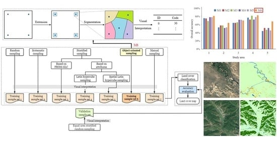
Figure 3.
Workflow of the object-oriented sampling.

Figure 4.
(a) Overall accuracy of each method; (b) F1 score of each method.

Figure 5.
Classification map.


Table 1.
Data for ecological zoning.
| Data/Product | Source | Resolution |
|---|---|---|
| Elevation | https://www.worldclim.org/ (accessed on 10 May 2021) | 30 s |
| Average temperature | 30 s | |
| Precipitation | 30 s | |
| Bioclimatic variables | 30 s | |
| MOD13Q1 | https://modis.gsfc.nasa.gov/ (accessed on 10 May 2021) | 250 m |
| MCD12Q1 | 500 m |
Table 2.
Band introduction of Sentinel-2.
| Name | Description | Resolution (m) |
|---|---|---|
| Band1 | Aerosols | 60 |
| Band2 | Blue | 10 |
| Band3 | Green | 10 |
| Band4 | Red | 10 |
| Band5 | Red Edge 1 | 20 |
| Band6 | Red Edge 2 | 20 |
| Band7 | Red Edge 3 | 20 |
| Band8 | NIR | 10 |
| Band8A | Red Edge 4 | 20 |
| Band9 | Water Vapor | 60 |
| Band11 | SWIR 1 | 20 |
| Band12 | SWIR 2 | 20 |
Table 3.
Land cover classification scheme.
| Name | Code | Description |
|---|---|---|
| Croplands | 10 | Cropland refers to the land where crops are planted. It has obvious characteristics of human-intensive activities and needs human activities to maintain for a long time. It includes rice fields, fallow, greenhouse, and orchards. |
| Forests | 20 | Forest refers to the land where woody plants grow mainly, the vegetation coverage rate is more than 15% and generally up to 60%, and the vegetation height is more than 3 m. It includes coniferous forests, broad-leaved forests, and mixed forests. |
| Grasslands | 30 | Grassland refers to the land where herbaceous plants are grown, with herbaceous coverage >15%, and arbor and shrub coverage <10%. It includes grazing-based shrub grassland and open forest grassland with canopy closure below 10%. |
| Shrublands | 40 | The height of the shrub is between 0.3 and 5 m. It includes canopy shrub with shrub canopy coverage >60% and sparse shrub with shrub canopy coverage of 10–60%. |
| Water bodies | 60 | Water bodies refer to natural waters and land used for water conservancy facilities. It includes lakes, reservoirs/ponds, rivers, and oceans. The spectral characteristics of the water body change greatly, and the water area changes with the seasons. |
| Impervious surfaces | 80 | Impervious surface refers to the land covered by buildings and other man-made structures, generally based on artificial covering materials, such as asphalt, concrete, sand, brick, glass, and other covering materials. |
| Barren land | 90 | Bare land refers to land where the vegetation coverage does not exceed 10%. It includes bare soil, sand, gravel, and rocks. |
Table 4.
Diversity of each sample set.
| Diversity | Study Area 1 | Study Area 2 | Study Area 3 | Study Area 4 | Study Area 5 |
|---|---|---|---|---|---|
| M1 | 0.2401 | 0.4542 | 0.2713 | 0.2810 | 0.1869 |
| M2 | 0.2490 | 0.4729 | 0.3185 | 0.2540 | 0.1692 |
| M3 | 0.2481 | 0.4992 | 0.2760 | 0.2357 | 0.1971 |
| M4 | 0.2473 | 0.4858 | 0.2700 | 0.2777 | 0.2700 |
| M5 | 0.2521 | 0.4883 | 0.3301 | 0.3218 | 0.1724 |
| M6 | 0.2600 | 0.5052 | 0.2859 | 0.3106 | 0.3266 |
| M7 | 0.2517 | 0.4956 | 0.2713 | 0.2926 | 0.3268 |
Publisher’s Note: MDPI stays neutral with regard to jurisdictional claims in published maps and institutional affiliations. |
© 2021 by the authors. Licensee MDPI, Basel, Switzerland. This article is an open access article distributed under the terms and conditions of the Creative Commons Attribution (CC BY) license (https://creativecommons.org/licenses/by/4.0/).
Share and Cite
MDPI and ACS Style
Li, C.; Ma, Z.; Wang, L.; Yu, W.; Tan, D.; Gao, B.; Feng, Q.; Guo, H.; Zhao, Y. Improving the Accuracy of Land Cover Mapping by Distributing Training Samples. Remote Sens. 2021, 13, 4594. https://doi.org/10.3390/rs13224594
AMA Style
Li C, Ma Z, Wang L, Yu W, Tan D, Gao B, Feng Q, Guo H, Zhao Y. Improving the Accuracy of Land Cover Mapping by Distributing Training Samples. Remote Sensing. 2021; 13(22):4594. https://doi.org/10.3390/rs13224594
Chicago/Turabian StyleLi, Chenxi, Zaiying Ma, Liuyue Wang, Weijian Yu, Donglin Tan, Bingbo Gao, Quanlong Feng, Hao Guo, and Yuanyuan Zhao. 2021. "Improving the Accuracy of Land Cover Mapping by Distributing Training Samples" Remote Sensing 13, no. 22: 4594. https://doi.org/10.3390/rs13224594
Note that from the first issue of 2016, this journal uses article numbers instead of page numbers. See further details here.