
Medium- (MR) and Very-High-Resolution (VHR) Image Integration through Collect Earth for Monitoring Forests and Land-Use Changes: Global Forest Survey (GFS) in the Temperate FAO Ecozone in Europe (2000–2015)

 , ,
, ,
Abstract
:
1. Introduction
2. Materials and Methods
2.1. Study Area
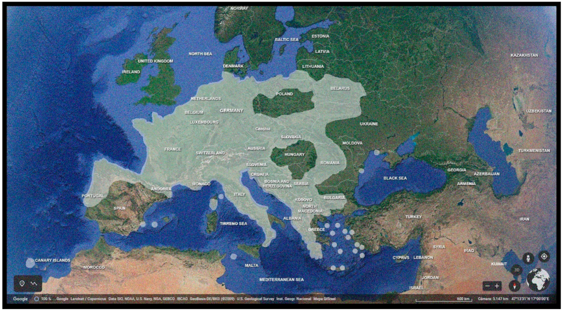
2.2. Data Collection
2.3. Data Processing
3. Results
4. Discussion
5. Conclusions
Author Contributions
Funding
Institutional Review Board Statement
Informed Consent Statement
Data Availability Statement
Acknowledgments
Conflicts of Interest
References
- Wang, L.; Tai, A.P.K.; Tam, C.-Y.; Sadiq, M.; Wang, P.; Cheung, K.K.W. Impacts of future land use and land cover change on mid-21st-century surface ozone air quality: Distinguishing between the biogeophysical and biogeochemical effects. Atmos. Chem. Phys. 2020, 20, 11349–11369. [Google Scholar] [CrossRef]
- Bajocco, S.; De Angelis, A.; Perini, L.; Ferrara, A.; Salvati, L. The impact of land use/land cover changes on land degradation dynamics: A mediterranean case study. Environ. Manag. 2012, 49, 980–989. [Google Scholar] [CrossRef]
- Canadell, J.G.; Raupach, M.R. Managing forests for change mitigation. Science 2008, 320, 1456. [Google Scholar] [CrossRef] [PubMed] [Green Version]
- Dale, V.H.; Joyce, L.A.; McNulty, S.; Neilson, R.P.; Ayres, M.P.; Flannigan, M.D.; Hanson, P.J.; Irland, L.C.; Lugo, A.E.; Peterson, C.J.; et al. Change and forest disturbances. BioScience 2001, 51, 723–734. [Google Scholar] [CrossRef] [Green Version]
- Alberdi, I.; Bender, S.; Riedel, T.; Avitable, V.; Boriaud, O.; Bosela, M.; Camia, A.; Cañellas, I.; Castro Rego, F.; Fischer, C.; et al. Assessing forest availability for wood supply in Europe. For. Policy Econ. 2020, 111, 102032. [Google Scholar] [CrossRef] [PubMed]
- Neumann, M.; Moreno, A.; Mues, V.; Härkönen, S.; Mura, M.; Bouriaud, O.; Lang, M.; Achten, W.M.J.; Thivolle-Cazat, A.; Bronisz, K.; et al. Comparison of carbon estimation methods for European forests. For. Ecol. Manag. 2016, 361, 397–420. [Google Scholar] [CrossRef]
- Hoscilo, A.; Levandowska, A. Mapping forest type and tree species on a regional scale using multi-temporal sentinel-2 data 2019. Remote Sens. 2019, 11, 929. [Google Scholar] [CrossRef] [Green Version]
- Plieninger, T.; Draux, H.; Fagerholm, N.; Bieling, C.; Bürgid, M.; Kizose, T.; Kuemmerlef, T.; Primdahla, J.P.; Verburg, H. The driving forces of landscape change in Europe: A systematic review of the evidence. Land Use Policy 2016, 57, 204–214. [Google Scholar] [CrossRef] [Green Version]
- Naranjo, J.M.; Loures, L.C.; Castanho, R.A.; Fernández, J.C.; Fernández-Pozo, L.; Neves, S.A.; Escórcio, P. Assessing land-use changes in european territories: A retrospective study from 1990 to 2012. In Land-Use. Assessing the Past, Envisioning the Future; Loures, L.C., Ed.; IntechOpen: London, UK, 2018; pp. 132–166. [Google Scholar]
- Barbati, A.; Corona, P.; Marchetti, M. A forest typology for monitoring sustainable forest management: The case of European Forest types. Plant Biosyst. 2007, 141, 93–103. [Google Scholar] [CrossRef]
- Barbati, A.; Marchetti, M.; Chirici, G.; Corona, P. European forest types and forest Europe SFM indicators: Tools for monitoring progress on forest biodiversity conservation. For. Ecol. Manag. 2014, 321, 145–157. [Google Scholar] [CrossRef] [Green Version]
- Barbati, A.; Salvati, R.; Ferrari, B.; Di Santo, D.; Quatrini, A.; Portoghesi, L.; Travaglini, D.; Iovino, F.; Nocentini, S. Assessing and promoting old-growthness of forest stands: Lessons from research in Italy. Plant Biosyst. 2012, 146, 167–174. [Google Scholar] [CrossRef]
- Mahmood, R.; Pielke, R.A., Sr.; Hubbard, K.G.; Niyogi, D.; Bonan, G.; Lawrence, P.; McNider, R.; McAlpine, C.; Etter, A.; Gameda, S.; et al. Impacts of land use/land cover change on and future research priorities. Am. Meteorol. Soc. 2010, 91, 37–46. [Google Scholar] [CrossRef]
- Giri, C.P. Remote Sensing of Land Use and Land Cover. Principles and Applications; CRC Press Taylor & Francis Group: Boca Raton, FL, USA, 2012. [Google Scholar]
- Feranec, J.; Jaffrain, G.; Soukup, T.; Hazeu, G. Determining changes and flows in European landscapes 1990–2000 using CORINE land cover data. Appl. Geogr. 2010, 30, 19–35. [Google Scholar] [CrossRef]
- Chen, J.; Cao, X.; Peng, S.; Ren, H. Analysis and applications of globeland30: A review. Int. J. Geo-Inf. 2017, 6, 230. [Google Scholar] [CrossRef] [Green Version]
- Oreti, L.; Giuliarelli, D.; Tomao, A.; Barbati, A. Object oriented classification for mapping mixed and pure forest stands using very-high resolution imagery. Remote Sens. 2021, 13, 2508. [Google Scholar] [CrossRef]
- Estel, S.; Kuemmerle, T.; Alcántara, C.; Levers, C.; Prishchepov, A.; Hostert, P. Mapping farmland abandonment and recultivation across Europe using MODIS NDVI time series. Remote Sens. Environ. 2015, 163, 312–325. [Google Scholar] [CrossRef]
- dAndrimont, R.; Yordanov, M.; Martinez-Sanchez, L.; Eiselt, B.; Palmieri, A.; Dominici, P.; Gallego, J.; Reuter, H.I.; Joebges, C.; Lemoine, G.; et al. Harmonised LUCAS in-situ land cover and use database for field surveys from 2006 to 2018 in the European Union. Sci. Data 2020, 7, 352. [Google Scholar] [CrossRef] [PubMed]
- Bey, A.; Sanchez-Paus Díaz, A.; Maniatis, D.; Marchi, G.; Mollicone, D.; Ricci, S.; Bastin, J.B.; Moore, R.; Federici, S.; Rezende, M.; et al. Collect earth: Land use and land cover assessment through augmented visual interpretation. Remote Sens. 2016, 8, 807. [Google Scholar] [CrossRef] [Green Version]
- FAO. Sustainable Forest Management (SFM) Toolbox. Available online: http://www.fao.org/sustainable-forest-management/toolbox/tools/tool-detail/en/c/411199/ (accessed on 20 September 2021).
- Bastin, J.F.; Berrahmouni, N.; Grainger, A.; Maniatis, D.; Mollicone, D.; Moore, R.; Patriarca, C.; Picard, N.; Sparrow, B.; Abraham, E.M.; et al. The extent of forest in dryland biomes. Science 2017, 356, 635–638. [Google Scholar] [CrossRef] [PubMed] [Green Version]
- Martin-Ortega, P.; Picard, N.; García-Montero, L.G.; del Río, S.; Penas, A.; Marchetti, M.; Lasserre, B.; Ozdemir, E.; García-Robredo, F.; Pascual, C.; et al. Importance of Mediterranean forests. In State of Mediterranean Forests 2018, 1st ed.; Food and Agriculture Organization of the United Nations, Plan Bleu, Eds.; Food and Agriculture Organization of the United Nations: Rome, Italy; Plan Bleu: Marseille, France, 2018; pp. 31–50. [Google Scholar]
- FAO-FRA. Global Forest Resources Assessment 2000: Main Report, 1st ed.; Food and Agriculture Organization of the United Nations: Rome, Italy, 2001; pp. 1–511. Available online: http://www.fao.org/3/Y1997E/Y1997E00.htm (accessed on 20 September 2021).
- Spiecker, H. Silvicultural management in maintaining biodiversity and resistance of forests in Europe-temperate zone. J. Environ. Manag. 2003, 67, 55–65. [Google Scholar] [CrossRef]
- Frison, P.-L.; Fruneau, B.; Kmiha, S.; Soudani, K.; Dufrêne, E.; Le Toan, T.; Koleck, T.; Villard, L.; Mougin, E.; Rudant, J.-P. Potential of sentinel-1 data for monitoring temperate mixed forest phenology. Remote Sens. 2018, 10, 2049. [Google Scholar] [CrossRef] [Green Version]
- García-Montero, L.G.; Pascual, C.; Sanchez-Paus Díaz, A.; Martín-Fernández, S.; Martín-Ortega, P.; García-Robredo, F.; Calderón-Guerrero, C.; Patriarca, C.; Mollicone, D. Land use sustainability monitoring: “Trees outside forests” in temperate FAO-Ecozone (oceanic, continental, and Mediterranean) in Europe (2000–2015). Sustainability 2021, 13, 10175. [Google Scholar] [CrossRef]
- FAO. Global Ecological Zones for FAO Forest Reporting: 2010 Update; FAO: Rome, Italy, 2012. [Google Scholar]
- Raši, R. State of Europe’s forests 2020. In Proceedings of the Ministerial Conference on the Protection of Forests in Europe, Bratislava, Slovakia, 14–15 April 2020; pp. 1–394. [Google Scholar]
- Eurostat. Land Cover Statistics. Available online: https://ec.europa.eu/eurostat/statistics-explained/index.php?title=Land_cover_statistics#Land_cover_in_the_EU (accessed on 25 September 2021).
- Négre, F. The European Union and Forests. Available online: https://www.europarl.europa.eu/factsheets/en/sheet/105/the-european-union-and-forests (accessed on 25 September 2021).
- EC European Comission. Political Agreement on New Common Agricultural Policy: Fairer, Greener, More Flexible. Available online: https://ec.europa.eu/commission/presscorner/detail/en/IP_21_2711 (accessed on 25 September 2021).
- EC European Comission. How Have European Forests Evolved over the Past 30 Years? Available online: https://ec.europa.eu/jrc/en/science-update/how-have-european-forests-evolved-over-past-30-years (accessed on 25 September 2021).
- Senf, C.; Pflugmacher, D.; Zhiqiang, Y.; Sebald, J.; Knorn, J.; Neumann, M.; Hostert, P.; Seidl, R. Canopy mortality has doubled in Europes temperate forests over the last three decades. Nat. Commun. 2018, 9, 4978. [Google Scholar] [CrossRef]
- Kautz, M.; Meddens, A.J.H.; Hall, R.J.; Arneth, A. Biotic disturbances in Northern Hemisphere forests—A synthesis of recent data, uncertainties and implications for forest monitoring and modelling. Glob. Ecol. Biogeogr. 2017, 26, 533–552. [Google Scholar] [CrossRef]
- Cohen, W.B.; Yang, Z.; Stehman, S.V.; Schroeder, T.A.; Bell, D.M.; Masek, J.G.; Huang, C.; Meigs, G.W. Forest disturbances across the conterminous United States from 1985–2012: The emerging dominance of forest decline. For. Ecol. Manag. 2016, 360, 242–252. [Google Scholar] [CrossRef]
- García-Montero, L.G. Project “Collecting Data through Collect Earth Tools on Southern Europe Dryland Zones in the Context of Global Forest Survey Project (GFS)” in the Framework of the FAO Project GCP/GL0/553/GER (BMU) Global Forest Survey (GFS); Universidad Politécnica de Madrid: Madrid, Spain, 2015. [Google Scholar]
- García-Montero, L.G.; Pascual, C.; Calderón, C.; García-Robredo, F. Project “Collecting Data through Collect Earth Tools in Europe and North America Zones in the Context of the Pilot on Global Assessment on Trends in Tree Cover/Land Use " in the Framework of the World Forest Open Date Initiative" (GCP/GL0/553/GER (BMU) Global Forest Survey GFS); Universidad Politécnica de Madrid: Madrid, Spain, 2016. [Google Scholar]
- FAO. Global Forest Survey. Available online: http://www.fao.org/in-action/global-forest-survey/en/ (accessed on 10 September 2020).
- Saah, D.; Johnson, G.; Ashmall, B.; Tondapu, G.; Tenneson, K.; Patterson, M.; Poortinga, A.; Markert, K.; Quyen, N.H.; San Aung, K.; et al. Collect earth: An online tool for systematic reference data collection in land cover and use applications. Environ. Model. Softw. 2019, 118, 166–171. [Google Scholar] [CrossRef]
- IPCC. Good Practice Guidance for Land Use, Land-Use Change and Forestry; Institute for Global Environmental Strategies: Hayama, Japan, 2003; p. 590. [Google Scholar]
- Martínez, S.; Mollicone, D. From land cover to land use: A methodology to assess land use from remote sensing data. Remote Sens. 2012, 4, 1024–1045. [Google Scholar] [CrossRef] [Green Version]
- FAO-FRA. Global Forest Resources Assessment 2015, 2nd ed.; Food and Agriculture Organization of the United Nations: Rome, Italy, 2016; pp. 1–253. [Google Scholar]
- FAO-FRA. Global Forest Resources Assessment 2020: Main Report, 1st ed.; Food and Agriculture Organization of the United Nations: Rome, Italy, 2020; pp. 1–186. [Google Scholar]
- Cochran, W.G. Sampling Techniques, 3rd ed.; John Wiley and Sons: Hoboken, NJ, USA, 1991; pp. 1–448. [Google Scholar]
- Jackson, M.O. Social and Economic Networks; Princenton University Press: Princenton, NJ, USA, 2008; p. 504. [Google Scholar]
- Goldewijk, K.K. Estimating global land use change over the past 300 years: The HYDE database. Glob. Biogeochem. Cycles 2001, 15, 417–433. [Google Scholar] [CrossRef]
- Rhemtulla, J.M.; Mladenoff, D.J.; Clayton, M.K. Historical forest baselines reveal potential for continued carbon sequestration. Proc. Natl. Acad. Sci. USA 2009, 106, 6082–6087. [Google Scholar] [CrossRef] [Green Version]
- Václavík, T.; Rogan, J. Identifying trends in land use/land cover changes in the context of post-socialist transformation in Central Europe: A case study of the Greater Olomouc Region, Czech Republic. Gisci. Remote Sens. 2009, 46, 54–76. [Google Scholar] [CrossRef] [Green Version]
- Kuemmerle, T.; Müller, D.; Griffiths, P.; Rusu, M. Land use change in Southern Romania after the collapse of socialism. Reg. Environ. Chang. 2009, 9, 1–12. [Google Scholar] [CrossRef]
- Forest Europe; UNECE; FAO. State of Europes forests 2011. In Proceedings of the Status and Trends in Sustainable Forest. Ministerial Conference on the Protection of Forests in Europe, Oslo, Norway, 14–16 June 2011; pp. 1–259. [Google Scholar]
- Forest Europe. State of Europe’s forests 2015. In Proceedings of the Ministerial Conference on the Protection of Forests in Europe, Madrid, Spain, 20–21 October 2015; pp. 1–314. [Google Scholar]
- Nave, L.E.; Vance, E.D.; Swanston, C.W.; Curtis, P.S. Fire effects on temperate forest soil C and N storage. Ecol. Appl. 2011, 21, 1189–1201. [Google Scholar] [CrossRef] [PubMed] [Green Version]
- Guo, M.; Li, J.; Xu, J.; Wang, X.; He, H.; Wu, L. CO2 emissions from the 2010 Russian wildfires using GOSAT data. Environ. Pollut. 2017, 226, 60–68. [Google Scholar] [CrossRef]
- Haddad, N.M.; Brudvig, L.A.; Clobert, J.; Davies, K.F.; Gonzalez, A.; Holt, R.D.; Lovejoy, T.E.; Sexton, J.O.; Austin, M.P.; Collins, C.D.; et al. Habitat fragmentation and its lasting impact on Earths ecosystems. Sci. Adv. 2015, 1, e1500052. [Google Scholar] [CrossRef] [Green Version]
- Griffith, D.M.; Lehmann, C.E.R.; Strömberg, C.A.E.; Parr, C.L.; Pennington, R.T.; Sankaran, M.; Ratnam, J.; Still, C.J.; Powell, R.L.; Hanan, N.P.; et al. Comment on “The extent of forest in dryland biomes”. Science 2017, 358, 6365. [Google Scholar] [CrossRef] [PubMed] [Green Version]
- Schepaschenko, D.; Fritz, S.; See, L.; Laso Bayas, J.C.; Lesiv, M.; Kraxner, F.; Obersteiner, M. Comment on “The extent of forest in dryland biomes”. Science 2017, 358, eaao0166. [Google Scholar] [CrossRef] [PubMed] [Green Version]
- De la Cruz, M.; Quintana-Ascencio, P.F.; Cayuela, L.; Espinosa, C.I.; Escudero, A. Comment on “The extent of forest in dryland biomes”. Science 2017, 358, eaao0369. [Google Scholar] [CrossRef] [PubMed] [Green Version]


| IPCC Land Use | Plot Count (2000) | Plot % (2000) | Plot Count (2015) | Plot % (2015) | Total Net Increase in No. of Plots, TCL 2 (%) |
|---|---|---|---|---|---|
| Forest land | 4568 | 40.94 | 4617 1 | 41.37 1 | 0.43 |
| Cropland | 4184 | 37.49 | 4030 | 36.11 | −1.38 |
| Grassland | 1289 | 11.55 | 1323 | 11.86 | 0.31 |
| Settlement | 791 | 7.09 | 850 | 7.62 | 0.53 |
| Wetland | 154 | 1.38 | 158 | 1.42 | 0.04 |
| Other land | 173 | 1.55 | 181 | 1.62 | 0.07 |
| Total | 11,159 | 100 | 11,159 | 100 | 2.77 3 |
| Temperate FAO Ecozone | Type of Land Use | Plot Count (2015) | Plot Count (2000–2014) |
|---|---|---|---|
| Forest land | Mixed conifers and broadleaf | 1488 | 7 |
| Conifers | 1266 | 15 | |
| Broadleaf | 835 | 9 | |
| Mixed deciduous broadleaf | 548 | 6 | |
| Plantation 1 | 307 | 3 | |
| Riparian forest | 42 | - | |
| Gallery forest | 4 | - | |
| Other plantations 2 | 53 | 3 | |
| Plantation of poplars (Populus) 3 | 33 | - | |
| Plantation of eucalyptus trees 3 | 16 | - | |
| Total forest land subtype plots | 4592 | 43 | |
| Non-forest land use | Rainfed farming | 3265 | 77 |
| Pastureland | 1117 | 71 | |
| Irrigated crops | 560 | 9 | |
| Village | 329 | 1 | |
| Urban area | 240 | - | |
| Scrubland | 229 | 8 | |
| Orchard | 182 | 4 | |
| Infrastructure | 144 | 2 | |
| Rocks | 130 | 4 | |
| Built area | 120 | 2 | |
| Lake or permanent pond | 85 | - | |
| Permanent river or inland delta | 37 | - | |
| Snow or glacier | 32 | - | |
| Cultivation in flood zone | 21 | - | |
| Mine | 17 | - | |
| Sand | 11 | 3 | |
| Riparian vegetation | 9 | - | |
| Swamp in inorganic soil 4 | 8 | - | |
| Seasonal river | 7 | - | |
| Delta coastal | 6 | - | |
| Seasonal lake | 3 | - | |
| Rice plantation | 2 | - | |
| Peat | 1 | - | |
| Plantation of acacia trees 3 | 1 | - | |
| Available data | 11,148 | 224 | |
| No data | 11 | 10,935 | |
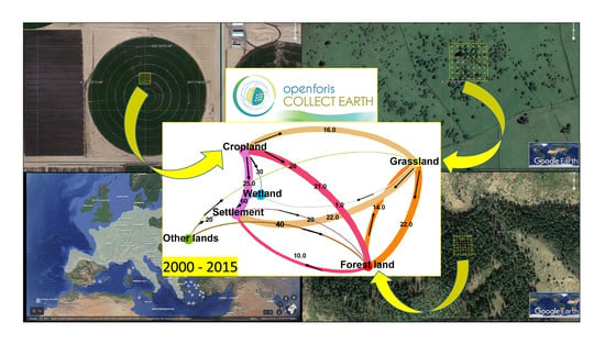
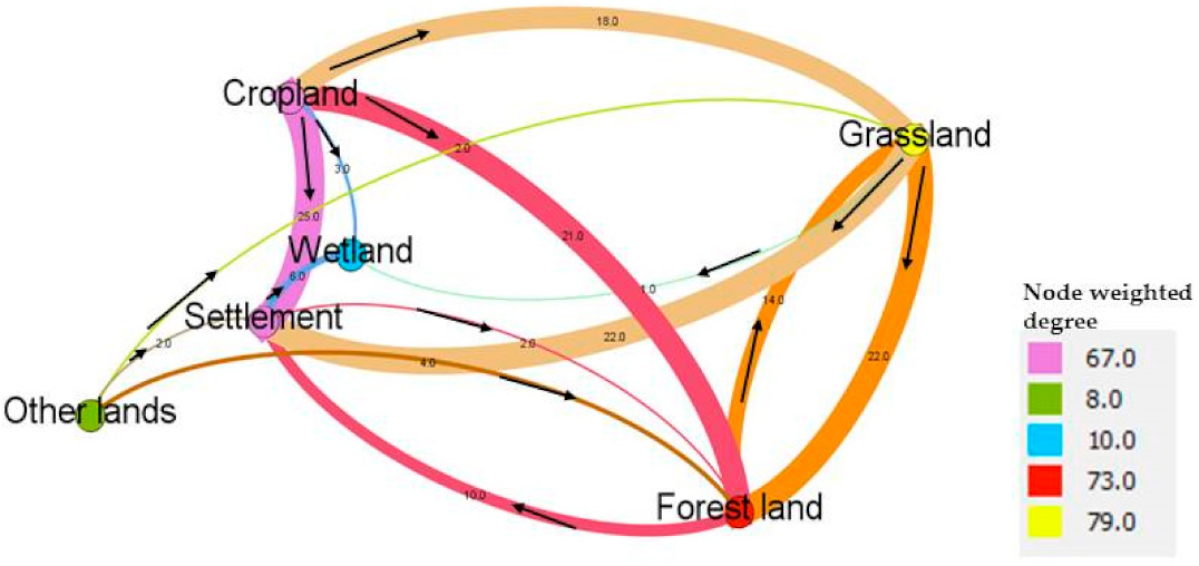
| Number of Plots | Forest Land | Grassland | Cropland | Settlement | Wetland | Other Land |
|---|---|---|---|---|---|---|
| Forest land | 0 | 14 | 0 | 10 | 0 | 0 |
| Grassland | 22 | 0 | 0 | 22 | 1 | 0 |
| Cropland | 21 | 18 | 0 | 25 | 3 | 0 |
| Settlement | 2 | 0 | 0 | 0 | 6 | 0 |
| Wetland | 0 | 0 | 0 | 0 | 0 | 0 |
| Other land | 4 | 2 | 0 | 2 | 0 | 0 |
| Land Use | Degree | In Degree | Out Degree | Weighted Degree |
|---|---|---|---|---|
| Forest land | 6 | 4 | 2 | 73 |
| Grassland | 6 | 3 | 3 | 79 |
| Cropland | 4 | 0 | 4 | 67 |
| Settlement | 6 | 4 | 2 | 67 |
| Wetland | 3 | 3 | 0 | 10 |
| Other land | 3 | 0 | 3 | 8 |
| Average per node | 4.65 | - | - | 50.66 |
| Type of Land Use (2015) | Disturbance Kind | Plot Count | % Relative to the Type of Land Use (2015) | % Total Available Data (10,340 Plots) |
|---|---|---|---|---|
| Forest land | None | 3930 | 91.89 | 38.01 |
| Tree felling | 237 | 5.54 | 2.29 | |
| Pastoralism | 41 | 0.96 | 0.40 | |
| Flooding | 14 | 0.33 | 0.14 | |
| Fire | 6 | 0.14 | 0.06 | |
| Mining | 5 | 0.12 | 0.05 | |
| Storm | 4 | 0.09 | 0.04 | |
| Non identified | 40 | 0.94 | 0.39 | |
| Cropland | None | 3527 | 95.66 | 34.11 |
| Other | 66 | 1.79 | 0.64 | |
| Tree felling | 53 | 1.44 | 0.51 | |
| Pastoralism | 30 | 0.81 | 0.29 | |
| Flooding | 9 | 0.24 | 0.09 | |
| Mining | 2 | 0.05 | 0.02 | |
| Other land | None | 163 | 94.22 | 1.58 |
| Other | 4 | 2.31 | 0.04 | |
| Mining | 3 | 1.73 | 0.03 | |
| Tree felling | 1 | 0.58 | 0.01 | |
| Pastoralism | 1 | 0.58 | 0.01 | |
| Flooding | 1 | 0.58 | 0.01 | |
| Grassland | None | 950 | 76.18 | 9.19 |
| Pastoralism | 236 | 18.93 | 2.28 | |
| Tree felling | 28 | 2.25 | 0.27 | |
| Other | 21 | 1.68 | 0.20 | |
| Flooding | 11 | 0.88 | 0.11 | |
| Storm | 1 | 0.08 | 0.01 | |
| Wetland | None | 126 | 85.71 | 1.22 |
| Flooding | 15 | 10.20 | 0.15 | |
| Other | 5 | 3.40 | 0.05 | |
| Pastoralism | 1 | 0.68 | 0.01 | |
| Settlement | None | 707 | 87.39 | 6.84 |
| Other | 61 | 7.54 | 0.59 | |
| Tree felling | 17 | 2.10 | 0.16 | |
| Mining | 16 | 1.98 | 0.15 | |
| Pastoralism | 8 | 0.99 | 0.08 | |
| All types | Disturbed plots | 937 | - | 9.06 |
| Available data | 10,340 | - | 100 | |
| No data | 819 | - | - |
| Subtypes of Forest Land (2015) | Disturbance Kind | Plot Count | % |
|---|---|---|---|
| Conifers (11.23%) 1 | None | 1065 | 91.73 |
| Tree felling | 73 | 6.29 | |
| Other | 10 | 0.86 | |
| Pastoralism | 7 | 0.60 | |
| Fire | 4 | 0.34 | |
| Mining | 2 | 0.17 | |
| Subtotal | 1161 | 100 | |
| Mixed conifers (0.70%) 1 | None | 68 | 94.44 |
| Tree felling | 4 | 5.56 | |
| Subtotal | 72 | 100 | |
| Broadleaf (7.84%) 1 | None | 765 | 93.97 |
| Tree felling | 22 | 2.71 | |
| Pastoralism | 20 | 2.46 | |
| Other | 2 | 0.25 | |
| Mining | 1 | 0.12 | |
| Flooding | 1 | 0.12 | |
| Subtotal | 811 | 100 | |
| Mixed conifer and broadleaf (13.03%) 1 | None | 1266 | 93.69 |
| Tree felling | 55 | 4.08 | |
| Other | 14 | 1.04 | |
| Pastoralism | 5 | 0.37 | |
| Flooding | 4 | 0.30 | |
| Storm | 2 | 0.15 | |
| Mining | 1 | 0.07 | |
| Subtotal | 1347 | 100 | |
| Mixed deciduous broadleaf (4.85%) 1 | None | 464 | 92.43 |
| Tree felling | 24 | 4.78 | |
| Pastoralism | 6 | 1.20 | |
| Other | 6 | 1.20 | |
| Mining | 1 | 0.20 | |
| Flooding | 1 | 0.20 | |
| Subtotal | 502 | 100 | |
| Plantation of poplars (Populus) (0.83%) 1 | None | 26 | 89.66 |
| Tree felling | 3 | 10.34 | |
| Subtotal | 29 | 100 | |
| All forest subtypes | Available data | 4174 | - |
| No data | 443 | - | |
| Total number of analyzed plots in the study area | - | 10,340 | - |
| Subtypes of Forest Land (2015) | Disturbance Kind | Plot Count | % |
| Plantation of conifers (5.44%) 2 | Tree felling | 42 | 21.99 |
| Fire | 1 | 0.52 | |
| Other | 1 | 0.52 | |
| None | 145 | 75.92 | |
| Storm | 2 | 1.05 | |
| Subtotal | 191 | 100% | |
| Plantation of Eucalyptus trees (0.46%) 2 | Tree felling | 8 | 50.00 |
| None | 8 | 50.00 | |
| Subtotal | 16 | 100% | |
| Riparian forest (0.40%) 2 | None | 35 | 85.37 |
| Flooding | 6 | 14.63 | |
| Subtotal | 41 | 100% | |
| Gallery forest (0.04%) 2 | None | 3 | 75.00 |
| Flooding | 1 | 25.00 | |
| Subtotal | 4 | 100% | |
| All forest subtypes | Available data | 4174 | - |
| No data | 443 | - | |
| Total number of analyzed plots | - | 11,159 | - |
Publisher’s Note: MDPI stays neutral with regard to jurisdictional claims in published maps and institutional affiliations. |
© 2021 by the authors. Licensee MDPI, Basel, Switzerland. This article is an open access article distributed under the terms and conditions of the Creative Commons Attribution (CC BY) license (https://creativecommons.org/licenses/by/4.0/).
Share and Cite
García-Montero, L.G.; Pascual, C.; Martín-Fernández, S.; Sanchez-Paus Díaz, A.; Patriarca, C.; Martín-Ortega, P.; Mollicone, D. Medium- (MR) and Very-High-Resolution (VHR) Image Integration through Collect Earth for Monitoring Forests and Land-Use Changes: Global Forest Survey (GFS) in the Temperate FAO Ecozone in Europe (2000–2015). Remote Sens. 2021, 13, 4344. https://doi.org/10.3390/rs13214344
García-Montero LG, Pascual C, Martín-Fernández S, Sanchez-Paus Díaz A, Patriarca C, Martín-Ortega P, Mollicone D. Medium- (MR) and Very-High-Resolution (VHR) Image Integration through Collect Earth for Monitoring Forests and Land-Use Changes: Global Forest Survey (GFS) in the Temperate FAO Ecozone in Europe (2000–2015). Remote Sensing. 2021; 13(21):4344. https://doi.org/10.3390/rs13214344
Chicago/Turabian StyleGarcía-Montero, Luis Gonzaga, Cristina Pascual, Susana Martín-Fernández, Alfonso Sanchez-Paus Díaz, Chiara Patriarca, Pablo Martín-Ortega, and Danilo Mollicone. 2021. "Medium- (MR) and Very-High-Resolution (VHR) Image Integration through Collect Earth for Monitoring Forests and Land-Use Changes: Global Forest Survey (GFS) in the Temperate FAO Ecozone in Europe (2000–2015)" Remote Sensing 13, no. 21: 4344. https://doi.org/10.3390/rs13214344