Article

Characterizing Leaf Nutrients of Wetland Plants and Agricultural Crops with Nonparametric Approach Using Sentinel-2 Imagery Data

1
School of Geography, Archaeology and Environmental Studies, University of the Witwatersrand, Johannesburg 2000, South Africa
2
Institute for Water Studies, Department of Earth Science, University of the Western Cape, Cape Town 7535, South Africa
3
Geoinformation Science Division, Agricultural Research Council-Institute for Soil, Climate and Water, Pretoria 0083, South Africa
4
Centre for Geoinformation Science, Department of Geography, Geoinformatics and Meteorology, University of Pretoria, Pretoria 0001, South Africa
5
Department of Geography, Environmental Studies and Tourism, University of the Western Cape, Cape Town 7535, South Africa
*
Author to whom correspondence should be addressed.
Remote Sens. 2021, 13(21), 4249; https://doi.org/10.3390/rs13214249
Submission received: 26 July 2021 / Revised: 18 October 2021 / Accepted: 19 October 2021 / Published: 22 October 2021
(This article belongs to the Special Issue Remote Sensing for Water Resources and Environmental Management)

Abstract

:
In arid environments of the world, particularly in sub-Saharan Africa and Asia, floodplain wetlands are a valuable agricultural resource. However, the water reticulation role by wetlands and crop production can negatively impact wetland plants. Knowledge on the foliar biochemical elements of wetland plants enhances understanding of the impacts of agricultural practices in wetlands. This study thus used Sentinel-2 multispectral data to predict seasonal variations in the concentrations of nine foliar biochemical elements in plant leaves of key floodplain wetland vegetation types and crops in the uMfolozi floodplain system (UFS). Nutrient concentrations in different floodplain plant species were estimated using Sentinel-2 multispectral data derived vegetation indices in concert with the random forest regression. The results showed a mean R2 of 0.87 and 0.86 for the dry winter and wet summer seasons, respectively. However, copper, sulphur, and magnesium were poorly correlated (R2 ≤ 0.5) with vegetation indices during the summer season. The average % relative root mean square errors (RMSE’s) for seasonal nutrient estimation accuracies for crops and wetland vegetation were 15.2 % and 26.8%, respectively. There was a significant difference in nutrient concentrations between the two plant types, (R2 = 0.94 (crops), R2 = 0.84 (vegetation). The red-edge position 1 (REP1) and the normalised difference vegetation index (NDVI) were the best nutrient predictors. These results demonstrate the usefulness of Sentinel-2 imagery and random forests regression in predicting seasonal, nutrient concentrations as well as the accumulation of chemicals in wetland vegetation and crops.

1. Introduction

Wetlands in South Africa cover about 2.9 million hectares and about 2.4% of the country’s land area [1]. They are recognised as highly valuable natural resources that sustain the livelihoods of local communities by providing a wide-ranging ecosystem goods and services that include, wild fruits, vegetables, rice and water purification [2,3]. They also mediate the adverse effects of extreme weather conditions [4] by attenuating floods and slowing down the speed of water movement [5]. Despite their valued recognition, the rate of wetland degradation worldwide and in SA remains high [6,7].
In South Africa, wetlands are some of the most threatened ecosystems, with ~50% of them in a critically endangered state [1]. Although they are vital for the livelihoods of rural communities [8], their sustainability is being threatened by the increasing incidence of climate change-driven droughts and frequent rainfall failures [9]. In sub-Saharan countries including Ethiopia, Kenya, Malawi, Tanzania, and Zambia, wetland cultivation is a recognised and common practice in arid environments [10] that generates about 37% of consumed food and 55% of cash income per household [11]. In Zimbabwe for example, Nyamadzawo, et al. [12] compared wetland gardens against upland fields and observed that more harvests from wetland gardens (2–3 t ha−1) compared to upland fields (1 t ha−1). Despite this higher productivity, wetland ecosystems are being adversely impacted by water extraction, urbanisation, infrastructure development, pollution, poor farming practices as well as droughts and climate variability.
Given their high agricultural productivity, and the water reticulation and other ecological roles, there is a need to explore spatially explicit techniques that can be used to assess and monitor nutrient enrichment in these ecosystems. This is essential because nutrient loading and contamination by different chemicals can disrupt the ecological functioning of these vital sub-systems. A selected example of this disruption is provided by Zhu, et al. [13] who report that an increase in foliar copper content is often associated with shrinkage of mesophyll cells and, concomitant destruction of the internal structure of a plant’s leaves and its physiological and structural characteristics. Although a detailed discussion of similar adverse effects is beyond the scope of this paper, it is apparent that better understanding of the foliar nutrient composition of wetland vegetation and crops is critical for informed adoption of eco-friendly management strategies. As vegetation links the physical environment and the upper levels of the food chain [14,15], these linkages need to be properly maintained because they determine the dynamics of nutrient circulation and physiological traits of plants in these systems.
Plants require at least fourteen mineral elements for adequate nutrition [16], lack of which reduces plant growth [17]. Six of these—nitrogen (N), phosphorus (P), potassium (K), calcium (Ca), magnesium (Mg), and sulphur (S)—are critically required by plants in adequate amounts [17]. Their presence at tolerable concentration levels in the plant can now be determined using remote sensing techniques [18,19,20,21,22,23,24,25,26,27]. However, considerable research still needs to be conducted on how the concentrations of these elements influence plant growth, as most of the research has tended to be narrowly focused on foliar nitrogen, phosphorus and potassium [18,19,20,21,22,23,24,25,26,27]. This bias can be explained by the dominant use of point-based sampling techniques and laboratory assaying, which are time-consuming and expensive These limitations can be overcome by tapping on the abilities of remote sensing techniques to cost-effectively provide quantitative estimates of foliar nutrient concentrations in wetland plants.
Nitrogen, phosphorus and potassium have been widely investigated using remote sensing techniques [28,29,30]. Although the literature indicates that these elements can be easily characterised using various techniques, other trace elements that are found in wetlands such as magnesium (Mg), copper (Cu), boron (B) and sulphur (S) are difficult to quantify. Remote sensing-based techniques provide a convenient way to overcome this limitation. This dexterity provides partial explanation of why we decided to use both in-situ and remotely sensing (RS) techniques to assess the foliar concentrations of these chemical elements and others.
The decision to couple these techniques was reasoned to be helpful because other researchers have also done this before using RS techniques and laboratory-based spectroscopy in order to cost-effectively maximise their usefulness [31,32,33,34]. Additional evidence to support this improvisation is provided by Li, et al. [32], who used hyperspectral data and laboratory analysis to characterise nitrogen and phosphorus concentrations in wetland plants. The majority of these studies have however mostly focused on grassland and dryland woody species [35]. Less effort has been exerted towards foliar nutrients like Cu, B, and S in wetland settings [36]. Although the traditional laboratory methods have been routinely used to provide the information that is required to guide wetland conservation and management [37], these methods are confounded by reliance on labour intensive, time consuming and costly field compilation and analysis of samples [38,39].
The use of hyperspectral RS data has proven to be capable of addressing these constraints and to further facilitate detailed characterisation of wetland plant nutrient concentrations [34]. Although these datasets are useful, they their usefulness is compromised by restricted temporal and spatial coverage with airborne hyperspectral sensors offering little for large scale applications compared to their space-borne equivalents because they are prohibitively expensive. This limitation causes hyperspectral data to be inflexible, inefficient, difficult to access and inappropriate for large scale mapping. To adequately monitor nutrient concentrations in wetland plants, a monitoring system that can be applied over optimum spatial and temporal scales is required. The use of freely available satellite imagery is a viable option as it enables cost-effective mapping and regular monitoring of inaccessible and extensive wetland areas [40,41]. Overall, the literature underscores the immense potentials of the medium resolution (M-res) datasets such as the WorldView-2, 3 and Sentinel-2 (S-2) in detecting variations in plant nutrient concentrations [1,42,43,44] compared to the costly high-resolution sensors [45].
In the last few years, S-2 is one of M-res datasets that has attracted a lot of interest by many researchers. Although launched recently in 2015, it has already proven to be highly useful for the monitoring of vegetation quality and macronutrients such as nitrogen and phosphorus [46,47,48]. Its high revisit period of 5 days, spatial resolutions of 10–60 m, systematic global acquisition and open access policy have made it the workhorse of local-level real-time plant nutrient monitoring. In addition to the visible and near-infrared (NIR) wavelengths, the S-2 includes three bands in the red edge region centred at 705, 740, and 775 nm, which are suitable for the characterisation of various plant traits and vegetation monitoring including macronutrients [19,26,48,49,50]. For instance, S-2 has been used to characterise the seasonal and spatial variations of the nitrogen and phosphorus ratio in the alpine grasslands of China at optimal accuracies of R2 0.49 and 0.59 and root mean square errors (RMSE) of 2.27 and 3.11 for the dry and wet seasons, respectively) [50]. Specifically, S-2 has 13 spectral bands comprising four bands, three bands and six bands with spatial resolutions of 10, 20 and 60 m that are centred at; (1) 496, 560, 665 and 835 nm (2), 703, 740, 783, 865, 1610 and 2202 nm, and (3), 443, 945 and 1373 nm respectively [51]. Because S-2 data can be accessed free of charge (https://scihub.copernicus.eu/25, accessed on June 2020), it has offered substantial opportunities for the mapping and monitoring of micro and vegetation macronutrients, especially in countries with limited access to spatial data due to financial and logistical constraints. However, unfortunately most of the studies that have sought to characterise foliar nutrients using S-2 remotely sensed data have tended to selectively focus on a narrow range of the primary nutrients notably, N, P, and K. This drawback argues for the need to explore ways through which the mapping of foliar micronutrients nutrients such as Mg, Cu, B and S, can be improved.
Evaluation of the nutritional requirements by different plants is becoming increasingly necessary because the scientific community is obliged to continue providing better means of enhancing the realisation of SDG goals that have a bearing to sustainable utilisation of the finite resources at our disposal. This asseveration is supported by the emergence of a community practice that is informed by the potential realisation of benefits from systematic utilisation of the rich RS datasets at our disposal and systematic use of the techniques that science has so far provided [50,52]. Accomplishing this is possible because RS provides robust techniques with demonstrated capabilities of providing the information required for meaningful realisation of SDGs, i.e., random forests (RF) ensemble, machine learning algorithms (MLAs) [53,54,55]. The use of MLAs, such as RF amongst others, in estimating nitrogen is a novel advancement that involves a fusion of several spectral vegetation indices in mapping leaf nutrient variations [56].
Although there is no machine learning method that is universally appropriate for estimating vegetation quality, several studies have evaluated the performance of the RF regression model (RF) in predicting the leaf nitrogen content of wetland vegetation [36,57]. RF has been demonstrated to be one of the most robust and widely used algorithms for this purpose [58,59,60,61,62]. The RF ensemble algorithm has been widely used in numerous studies to estimate plant foliar nutrient variations. This is so because, apart from being able to discern subtle variations in numerous variables, RF is able to identify the complex relationships between auto-correlated descriptors [63,64]. When implemented properly, RF offers additional advantages in that regardless of the sample size of the dataset used, it has a bootstrapping mechanism that accommodates utilisation of data implemented when drawing training data points for building trees for each model [
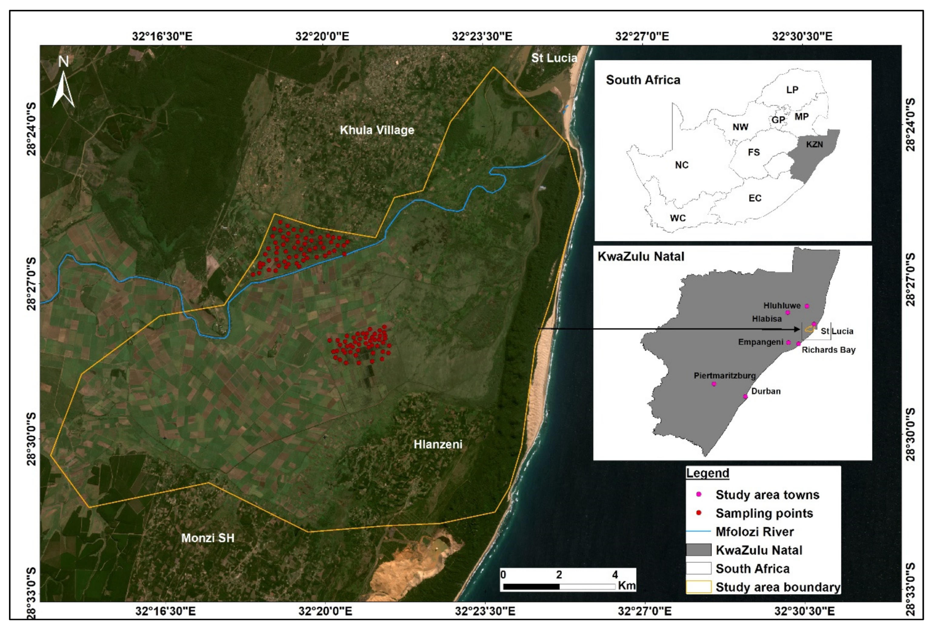
65]. It is in this regard that RF was perceived to be a suitable algorithm for estimating foliar nutrient concentrations in the floodplain wetlands of Northern KwaZulu Natal, South Africa. The underlying research question of the study was, can Sentinel-2 data in concert with RF be used to characterise the concentrations of N, K, Ca, Mg, P, S, Zn, B and Cu in the leaves of wetland natural vegetation? We attempted to answer this question by calculating Sentinel-2-derived vegetation indices for different herbaceous species in. The results showed that there is urgent need to explore techniques that can be used to provide unitary perspectives on how these and other challenges can be addressed. This investigation attempts to do this by providing a case illustration of how RF regression modelling can be used to (1) characterise the N, K, Ca, Mg, P, S, Zn, B and Cu foliar concentrations in different wetland vegetation species b) determining the key wavelengths that are important predictors in ascertaining the biochemical leaf foliar variations in these chemicals and (3) characterising seasonal variations in wetland plant leaf nutrient content.

2. Materials and Methods

2.1. Study Area

The uMfolozi floodplain (UFS) system is located in St Lucia, a town that is situated at 28°22′S and 32°25′E in Mtubatuba Local Municipality, South Africa. The uMfolozi River consists of two main tributaries, the Black uMfolozi; that rises at around 1500 m asl. in the north and the White uMfolozi that rises to an altitude of 1620 m asl. these two tributaries converge on the sea Around 50 km west of the mouth of the uMfolozi River. Because the catchment falls within the uMfolozi–Hluhluwe Nature Reserve, the bulk of the catchment comprises natural vegetation cover. Grasslands are about 60% of natural vegetation, with 21% and being classified as thicket and bush respectively. In less than a quarter of the uMfolozi catchment, natural vegetation comes under the dominant agriculture and commercial forestry land uses. The UF floodplain is predominantly used for sugar cane cultivation (65%), and the remaining designated as protected area under the iSimangaliso Park (previously known as St. Lucia Wetlands Park).
The uMfolozi River catchment drains a portion of 11,068 km2 of northern KwaZulu-Natal on Southern Africa’s eastern seaboard. The river’s surface geological layout consists of Lebombo rhyolite rock in the east and, Zululand/Maputaland rocks calcarenite, calcareous, limestone, and conglomerate formations in the north and south of the Indian Ocean respectively [66]. About 80% of the rainfall/precipitation occurs in the summer months, peaking between November and April [67]. Mean annual catchment precipitation ranges between 1288 mm in the coastal town of St. Lucia and 667 mm/a in the mid-upper catchment of the uMfolozi Game Reserve with ~914 mm/a occurring in the upper catchment in Nongoma. Mean annual evapotranspiration potential is normally more than double that of precipitation, with average amounts approximating 1800 mm/a [68]. Figure 1 shows the geographic location of the study area in KwaZulu Natal province, South Africa.

2.2. Field Data Collection

2.2.1. Plant Leaf Sampling

The datasets comprised leaf samples of major crops (Musa acuminate, Ipomoea batatas, sugarcane and Colocasia esculenta) and dominant wetland vegetation species (Phragmites australis, Cyperus papyrus and Cynodon dactylon). Sampling points were systematically generated to cover the study area’s footprint and leaves likewise selected following a sampling procedure that was designed to provide representative coverage of the sampling universe. Leaf samples were collected on the 12 March 2017 (wet/summer season) and 22 July 2017 (dry/winter season) respectively. During field investigation, the geographic positions of identifiable herbaceous species were recorded in spreadsheet inventories for further analysis and detailed verification of their geographic positions and species type
A Garmin Montana 650 global positioning system (GPS) with a rated positional accuracy of ±3 m, was used to measure the location of each plant where leaves were harvested. This was followed by randomised sampling of leaves at different crown levels (top, middle, and bottom) to avoid bias. Overall, a total of 76 leaf samples (38 for crops and 38 for vegetation) were collected in summer and 85 samples (40 for crops and 45 for vegetation) collected in winter and ~150 g of leaf material collected from each crop/plant. Leaf samples were then packed in labelled ziplock plastic bags and stored in a cooler box to preserve them during transportation to the laboratory. In the laboratory, the samples were oven-dried at 70 °C for at least 24 h and milled to particle sizes of <0.5 mm.

2.2.2. Chemical Analyses

In this study, six major elements required in large amounts by plants (nitrogen, phosphorus, potassium, calcium, magnesium and sulphur) [17] and three micronutrient elements required as trace amounts (boron, zinc and copper) [69] were chosen. The dry oxidation (Dumas) method was used to determine nitrogen [67] by igniting each leaf sample in oxygen at 950 °C to produce carbon dioxide, nitrogen gas and oxides of nitrogen. These gases were passed through silvered cobalt oxide and a column of copper at 650 °C to reduce the nitrogen oxides to nitrogen gas by removing excess O2. After removal of water vapour and CO2, the N2 gas was finally separated from other gases using gas chromatography, based on a helium carrier gas and detection by a thermal conductivity detector. The instrument was calibrated against the pure compound of known composition following standard procedures that been recommended for this purpose. The compound chosen for the calibration standard is phenylalanine which contains 8.48% N.
An aliquot of the digest solution was used for the inductively coupled plasma optical emission spectrometric (ICP-OES) instrument (Agilent Technologies, United States, North America) for the determination of K, Ca, Mg, P, S, Zn, B and Cu [70]. This is an Agilent 725 (700 series) simultaneous instrument which determines all the elements and wavelengths simultaneously. Thus, several of the elements may be determined at more than one wavelength allowing confirmation of the values with no increase in analysis time or consumption of digest solution. However, S was determined separately from the other elements after purging the optics of the instrument with Ar gas. This is due to the low wavelengths (<190 nm) used for detecting S and the problems caused by oxygen in the air at these very low wavelengths if the system is not purged. Each element was measured at one or two appropriate emission wavelengths that were chosen for their high sensitivity and lack of spectral interferences.

2.2.3. Image Compilation and Pre-Processing

Table 1 describes the characteristics of the S-2 images that were used and the numbers of sample sites from which leaf samples were collected during the wet (12 March 2017) and dry (22 July 2017) seasons.
The S-2 images were preferred because of their optimum spatial and spectral resolutions for leaf-nutrient characterisation and the availability of footprint coverages of the study area. The difference in the number of days between collection dates of samples and image acquisition dates for wet and dry periods were restricted to 15 and 4, respectively (Table 1) in order to enhance the acquisition of similar leaf nutrient concentrations by using samples at the same phenological stages. The images were atmospherically corrected to surface reflectance using the Sen2Cor plug-in tool provided in the Sentinel Application Platform (SNAP) toolbox, as illustrated in literature [71,72,73]. S-2 MSI has 13 spectral bands four at 10 m (blue (band 2), green (band 3), red (band 4), and NIR 1 (band 8)), six at 20 m (RE1 to 3 (band 5, 6 and 7), NIR-2 (band 8A), SWIR 1 (band 11) and 2 (band 12), and three at 60 m spatial resolution. Except for bands 1, 9 and 10, all S-2 MSI 10 and 20mbands were used in mapping foliar nutrients in this study. The 10 m bands were all resampled to a spatial resolution of 20 m before estimating the foliar nutrients. However, bands 1, 9, and 10 which have a spatial resolution of 60 m were excluded in this study because they are not suitable for vegetation applications. The images were classified in ArcGIS 10.6 by using 70% of the data that was collected during field investigation for signature compilation with the remaining 30% being reserved for classification accuracy assessment. Vegetation indices were then computed and used with the spectral bands to estimate leaf nutrient concentrations in wetland vegetation and crops growing by using several red edge based indices (Table 2).
Although a large and growing body of the literature has illustrated that vegetation indices outperform general wavebands in estimating vegetation attributes [80,81,82], in this study we combined the vegetation indices with spectral bands considering that very few of the aforementioned studies were conducted in wetlands. Vegetation indices were used in this study because of their robustness as illustrated in the literature [50,56,57,80,83,84,85]. They derive their robustness from two or more wavebands. These bands are often from two different regions of the electromagnetic spectrum. Their optimal performances have also been observed to be capable of circumventing the effects of the atmospheric noise, view/sun angle soil background, topographic effects and sensitivity to vegetation spectral and temporal attributes [86]. This and other considerations explain why Sentinel-2 wavebands were used in this investigation. The processes that were used for this purpose are summarised in Figure 2 which shows how satellite image data and field data were collected and combined in RF regression modelling.

2.3. Estimation of Nutrient Concentrations Using Random Forests Regression

RF was performed in the R statistical package to estimate the concentrations of nutrients in crops and wetland vegetation. RF is a blended model that is characterised by an enormous number of trees [59,87]. The model works by repeatedly splitting each tree (remotely sensed data in this study) into increasingly homogenous subsets at each node to produce a series of terminal nodes. In this study, the training of the regression model was based on 70% of the field data and new estimations determined by sensing the input down the tree and taking the means of the response variables (nutrient contents) and the remaining 30% was used for accuracy assessment as explained earlier.
Each regression tree in the RF algorithm is built using a subset of training samples that are independently selected by replacement of the original samples [88]. A subset of a few variables was randomly selected to determine the split in order to increase the robustness of the model by increasing diversity amongst trees and avoiding overfitting the model [88] and the RF predictor was finally constructed by taking the average of overall trees. The samples that are not utilised to grow the tree are referred to as Out of the Bag (OOB) data [59] which the algorithm uses to estimate accuracy by using the difference in the mean square errors to compute the OOB error estimate [71]. The explanatory power of each variable is determined by a Gini coefficient which measures the total decrease in node impurity (weighted by the probability of reaching that node) averaged across all trees. In this study, two hyperparameters were used to tune the models, that is the number of trees (ntree) and the number of variables randomly sampled as candidates at each split (mtry). It has to be pointed out that the adjustment of these hyperparameters did not significantly change the results hence these were held constant for various models considering the variability in the number of samples in stages 1 to 3 illustrated in Table 3.
Variable selection of the most important model parameters needed for accurate nutrient estimation was accomplished by implementing the backward feature elimination method [89,90]. The variable importance in RF determines various measures such as the importance of variables based on the Gini coefficient and permutation coefficient. The variation method is considered superior to other approaches because it uses OOB assessments [59]. RF assesses the variable importance of different factors by using the mean decrease in accuracy. Increased mean variability indicates greater importance for that particular variable, while low mean values indicate a lower influence in the model. The method works by generating all the variables of the input predictor and gradually removing input predictor variables with the least relative effect. Table 3 describes the experiments that were performed with S-2 MSI data to estimate nutrient concentrations in crops and wetland vegetation. More details on the RF regression ensemble are provided elsewhere [50,59,91,92].
To estimate nutrient concentrations, data analysis was done in three analysis stages (stage 1, 2, 3). Model input variables varied in each analytical phase. For analysis I, nutrient concentrations were estimated using Sentinel 2 MSI bands only. These were bands 2, 3, 4, 5, 6, 7, 8, 8A, 11 and 12, whereas, additional vegetation indices were computed and used as a stand-alone dataset to estimate nutrient concentrations. The following vegetation indices were computed; chlorophyll green (Cl.green), chlorophyll red edge (Cl.green), red edge position (REP 1, 2 and 3), simple ratio (SR 1, 2 and 3), the NDVI index, MERIS terrestrial chlorophyll index 1 (MTCI.1), modified normalised vegetation indices (nDVI (i.e., nDVI_Bγi_ Bγj)), as well as modified simple ratio vegetation indices (sR (i.e., sR_Bγi_ Bγj, where Bγi and Bγj are different Sentinel 2 MSI spectral bands)). The selected indices were computed based on all possible Sentinel 2 band combinations (10 spectral bands). Then S-2 MSI bands were then used as standalone model input variables except for the wet season (March) and the dry (July) seasons (Table 4 and Table 5). This was undertaken to determine the ability of Sentinel-2 MSI data in detecting the seasonal differences in leaf nutrient concentrations. For stage 2 analysis, we detected and characterised the year-round nutrient concentrations using pooled seasonal data which was categorised into two datasets (wetland vegetation and crops). In addition, spectral bands and vegetation indices were used separately to estimate the foliar nutrients (Table 6). For the third analysis, to assess the robustness of S-2 MSI data in detecting and characterising nutrient concentrations across all seasons (Figure 3), wet and dry season datasets were pooled into one dataset. Specifically, vegetation indices were used as standalone model input variables (Figure 3). All estimation models were evaluated by using the explained mean squared residual (MSR) variance (Var Expl (%), root mean square error (RMSE) and, RMSE %.
The RMSE% and the R2 were scaled between 0 and 100. To compute the RMSE%, all RMSEs from each model were normalised using the mean of each variable and then expressed as percentages [93,94]. The RMSE% has been widely used in the literature to compare different variable estimations [94,95,96] hence it was adopted and used in this study. The accuracies (RMSE % and in some instances with R2) of the training datasets were presented and used to conduct the Mann–Whitney U and the Student’s T tests. The Mann–Whitney U independent samples test was then used to test whether there were significant differences at α = 0.05 between the estimation accuracies (R2 and RMSE%) derived during the summer in relation to those derived from the winter crops and wetland vegetation, respectively (Table 6). The Mann–Whitney U Test was used following the data’s significant deviation from the normal distribution at α = 0.05 based on the Kolmogorov–Smirnov Test. Similarly, a Student’s t-test of independent samples was then used to assess whether the estimation accuracies derived from crops were significantly different from those derived from wetland vegetation presented in (Table 7) at α = 0.05 (Table 8). The Student’s t-test was used because the data did not significantly deviate from the normal distribution based on the Kolmogorov–Smirnov test. The raster calculator tool in ArcGIS 10.6 was used to map the spatial and temporal distributions of nutrients by utilizing the RF regression model outputs and essential variables (NDVI, REP1, and band 7) to characterize the studied nutrients. Figure 2. summarises the methods that were used to determine the accuracies of these calculations.

3. Results

3.1. Comparison of Single Bands and Vegetation Indices in Estimating Different Nutrients in Summer and Winter Seasons

Table 4 and Table 5 shows the seasonal accuracy levels (RMSE, R2, and RMSE %) for different nutrients that were investigated based on the raw bands and vegetation indices. The RMSE, which depicts the standard deviation of residuals, shows that the linear regression model based on vegetation indices performed better than raw bands. Using raw spectral bands, all of the RMSE values for both crops and vegetation in summer and winter were greater than of the vegetation indices (Table 4 and Table 5). As a result, the results of vegetation indices were used for further analysis of this study because of their lower prediction errors (RMSE values).
For both vegetation and crops, high R2 and low RMSE% were observed for all nutrients in winter (Table 4 and Table 5). For instance, Calcium (Ca) estimation in crops based on VIs exhibited an R2 of 0.73 and RMSE of 5889.75 (mg/kg) which was optimally estimated to an R2 of 0.95 and a RMSE of 39284.56 (mg/kg) (RMSE % = 12) based on vegetation indices in summer (Table 4). Meanwhile in winter Ca exhibited a R2 = 0.72 and a RMSE = 2289.59 mg/kg (RMSE % = 36) based on bands only. These accuracies improved to an R2 of 0.81, RMSE of 1582.82 mg/kg (RMSE % = 28). A similar trend was observed when estimating nutrients in wetland vegetation (Table 5). Specifically, poor accuracies of an R2 = 0.73, RMSE = 5889.75 mg/kg (RMSE % = 52) were attained when estimating Ca in wetland vegetation using only spectral bands during the summer. These accuracies improved when vegetation indices were used with an R2 of 0.95, RMSE of 3924.56 mg/kg and an RMSE % of 12. A similar trend was also observed in estimating Ca during the winter season. A R2 = 0.56, RMSE = 1684.49 mg/kg and a RMSE% = 29. An improvement in the accuracies was realised in estimating Ca in using bands only. Again, an improvement was observed when estimating Ca using the vegetation indices (R2 = 0.98, RMSE = 1498.356 mg/kg and a RMSE% = 25) during winter. The summer–winter RMSE percentages were higher in vegetation compared to crops and the differences in average values for both were significant (Table 6).
Table 6, Table 7 and Table 8 show seasonal mean comparisons of R2 and RMSE % nutrient estimations and seasonal nutrient estimation accuracies for crops and vegetation Table 8 shows R2 values and RMSE% for vegetation and crop types using pooled data.

3.2. Dry and Wet Season Crop and Vegetation Nutrient Estimation Using Pooled Data

In addition, the annual estimations of nutrient concentrations presented in Table 7 were used to calculate the statistics provided in Table 8. A higher mean R2 accuracy for nutrients across plant types was observed for vegetation (0.94) when compared to a mean R2 of 0.84 for crops (Table 8). The differences in the mean R2 values were significant. A higher percentage of RMSE (27) was observed for crops when compared to what was observed for vegetation (15). The difference between these vegetation types and crop RMSE values was significant. In all cases, measured and estimated nutrient concentrations were strongly correlated with R2 ranging from 0.98 for boron to 0.75 for magnesium. Although boron and magnesium showed a good correlation, both had high RMSE percentages.
Figure 2 is a composite summary of the performance of the statistical models that were used to relate foliar nutrients measured from the laboratory and data from S-2 images. Figure 3 shows the best fits for the model (in terms of R2 and RMSE %) arranged by performance. As it can be noted, the studied nutrients’ estimation performances were strong and very consistent, with R2 values ranging from 0.81 to 0.93. The nutrients, on the other hand, showed the opposite in terms of variability based on the RMSE%. However, it’s worth noting that lower RMSE values suggest a better model estimation fit. The RMSE percentages for different nutrients ranged from 14% to 29%. Zinc, potassium, sulphur, copper, and nitrogen were found to have low RMSE percentages ranging from 14% to 17%. The RMSE of calcium, boron, and magnesium were all high, with boron having the highest of 29 per cent. The overall findings revealed that several nutrients, such as calcium, boron, and magnesium, are poorly estimated, as evidenced by the RMSE per cent values.

3.3. Variable Importance Selection

The RF model was able to rank the variables by their estimation capabilities. Figure 3 shows important variables derived in estimating N, K, Ca, Mg, P, S, Zn, B and Cu. REP1 and NDVI were the most frequent vegetation indices that yielded optimal models of estimating foliar nutrients as indicated by their high % IncMSE in Figure 4.
Figure 5 illustrates the estimated spatial distributions of sulphur, potassium, magnesium, copper, nitrogen, phosphorus, zinc and boron. The lowest values correspond to areas with crop farming (dark red for waterbodies), higher values (dark green) represent the most developed vegetation (forest and grassland). It can be observed that nutrients have high concentrations in the eastern section of the study area, except for magnesium that showed high concentrations in the sugarcane infested area.

4. Discussion

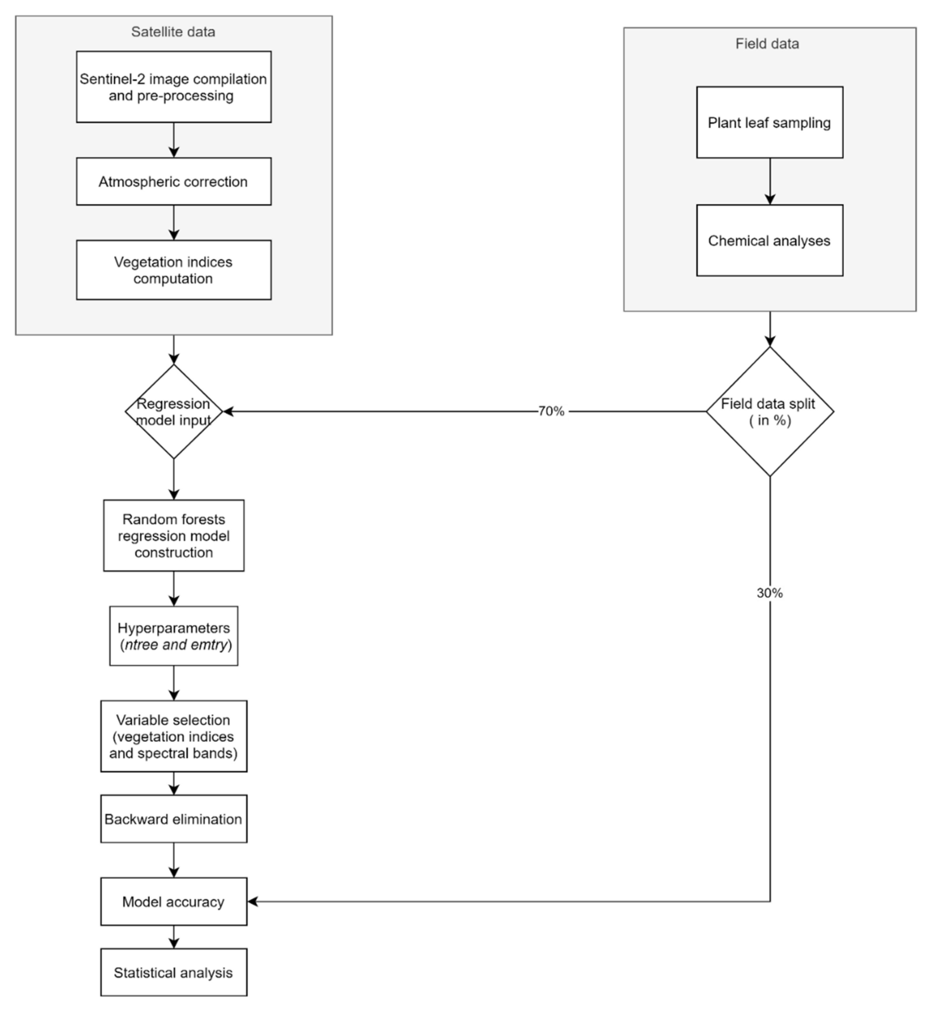
In this study, we used the RF algorithm and S-2 on both wetlands vegetation and crops and across seasons to estimate the concentrations of N, K, Ca, Mg, P, S, Zn, B and Cu. The results show that: (a) the RF model using S-2 can estimate foliar concentration across several nutrients and (b) S-2 can estimate nutrients across plant types and seasons. Derived S-2 vegetation indices such as NDVI and bands 2 and 7 performed well in estimating nutrients in crops and vegetation. Seasonal characterisation of nutrients was also successful which could be attributed to the variability of photosynthetic pigments such as chlorophyll [36]. However, the RF model performed poorly in estimating magnesium, and sulphur in the summer season. It also performed poorly in estimating calcium, magnesium, phosphorus and boron in wetland vegetation across the seasons as demonstrated by high RMSE %s. This can be attributed to easy leaching and increased mobility of these nutrients that might have caused the decrease of their concentration during the high rainfall period hence weak correlation with S-2. Phenology is also an important factor in this result because most vegetation indices such as NDVI, especially red edge-based indices, rely on the vigour and greenness of the vegetation. Osco, et al. [97] also found nutrients like Mg, S, P, K and Ca presented inferior performances compared to nutrients such as nitrogen, zinc etc. Another contribution of this work is that it was possible to identify wavelengths and spectral regions that contributed most to nutrient estimation.
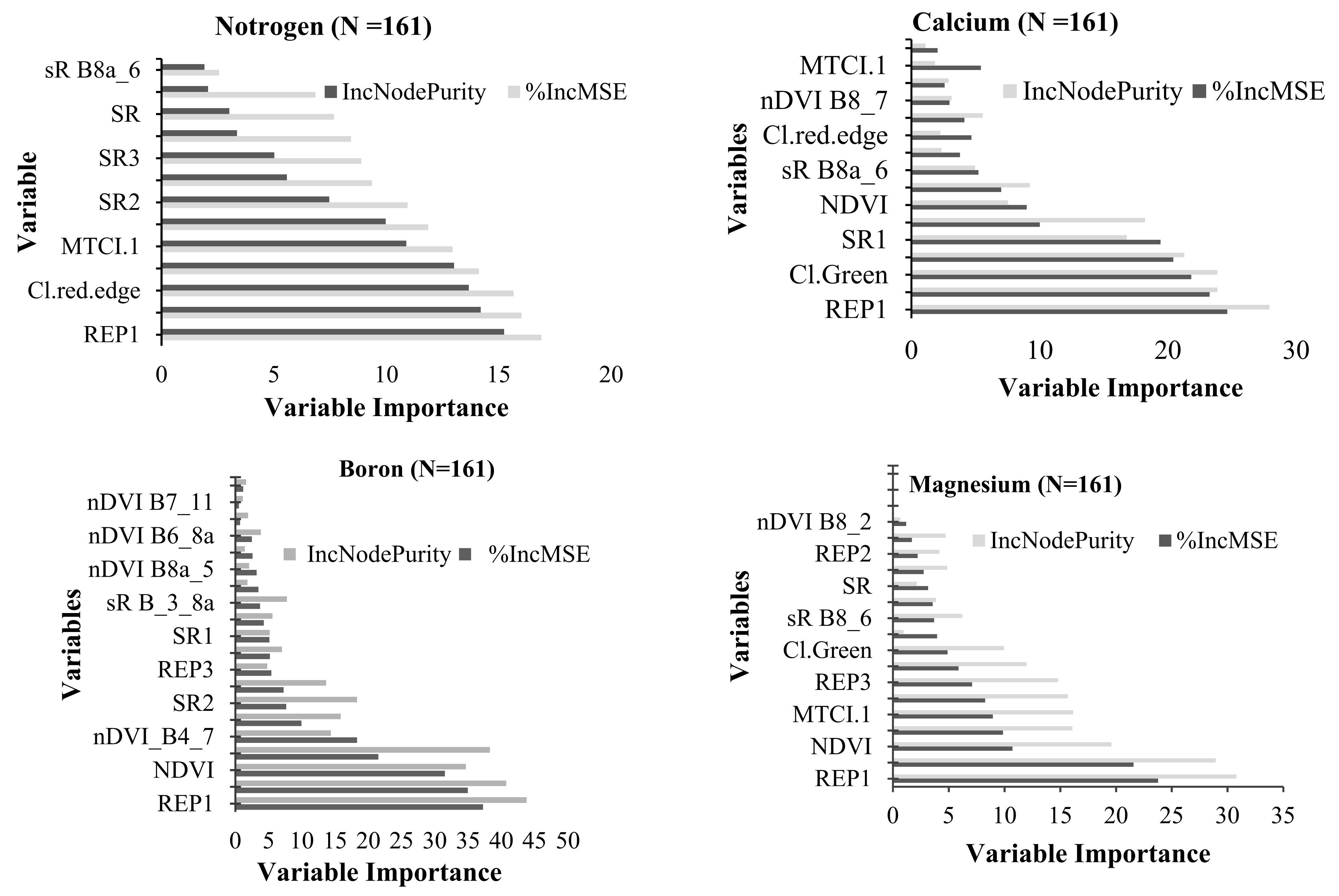
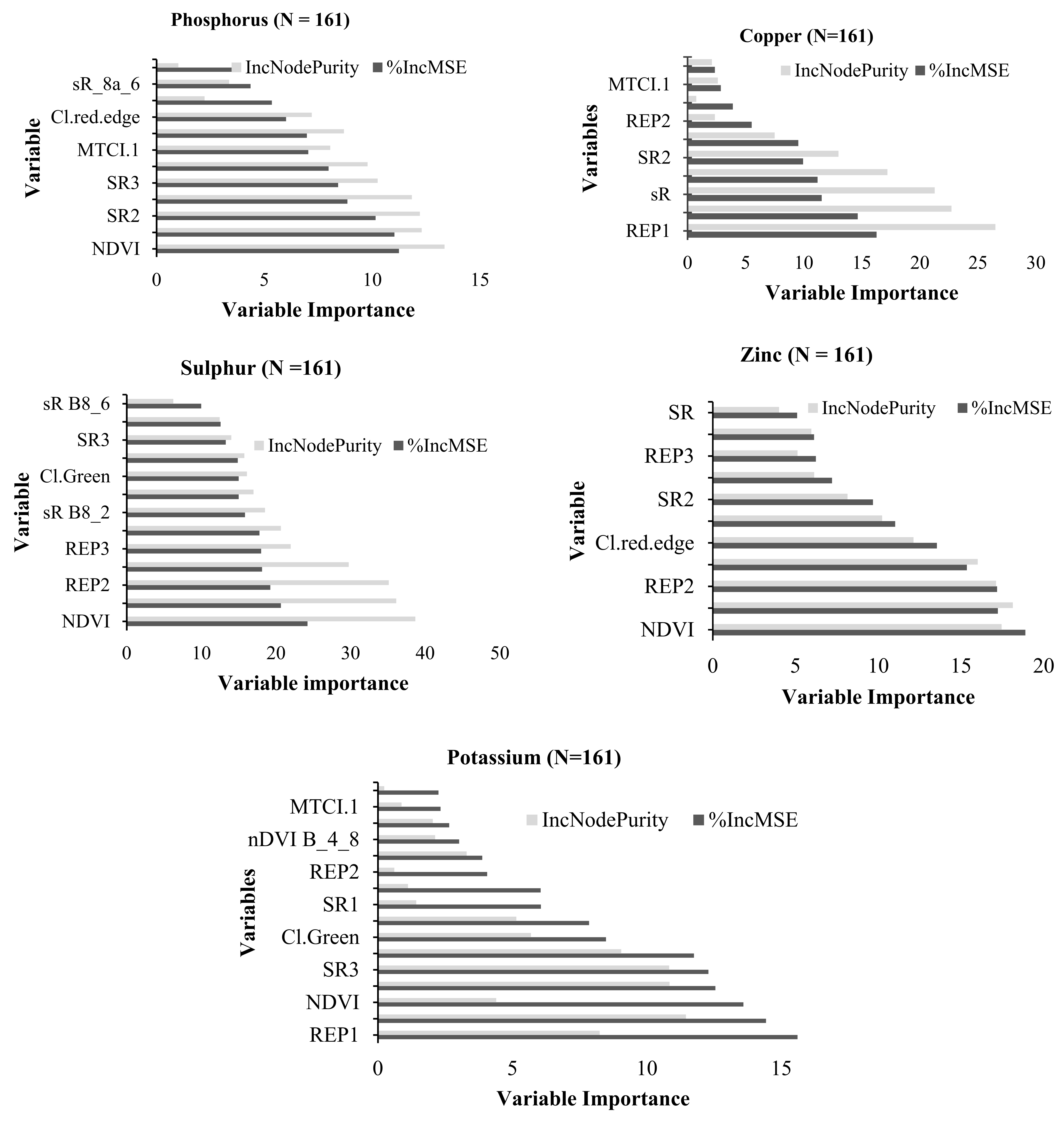
A combination of vegetation indices and spectral bands was found to be robust when compared to the raw spectral bands. As outlined above, the infusion of vegetation spectral indices proved to be important in the evaluation of the most studied nutrients [98,99,100]. Different indices and bands that were key to estimating nutrient concentrations include the red edge position, NDVI and band 2 (Figure 2). This observation implies that different nutrients can be estimated by these different variables. In this study, the key variables that were important in estimating most of the nutrients including nitrogen, potassium, calcium, boron and copper were the red edge position 1 computed from the NIR and red edge position bands followed by NDVI for estimating P and S. Similar findings were observed in Bush Buck Ridge, Mpumalanga, South African savannah grass where canopy nitrogen was correlated to NIR spectral region [101]. In similar findings were also found in North American forests where canopy nitrogen was correlated to both the NIR spectral region as well as NIR-based vegetation indices including NDVI [102,103].
The sensitivity of red edge bands to potassium, calcium, copper and nitrogen was not surprising. Studies by other researchers confirm the strong correlation between nitrogen concentrations and red edge bands [18,51,104,105]. The red edge is considered as the surrogate measure of vegetation chlorophyll content [51,106,107]. Therefore, in this study, an expectation of the magnesium concentration to be strongly estimated in the red edge bands was not questionable. Magnesium is located in the central of the chlorophyll molecule and it is regarded as the activator of some enzymes in plants [108]. The results by [109,110] found the NIR region to be the best in estimating magnesium concentrations. NDVI computed from red and NIR bands showed to be the key variable in estimating phosphorus and sulphur concentrations. This is similar to the findings of Lisboa, et al. [111], who found NDVI to be a useful tool in estimating nitrogen and phosphorus concentrations in sugarcane crops. Several studies have used these indices (NIR spectral region and NDVI) to study heavy metals in plants [112,113,114].

4.1. Estimation of Nutrients Using the RF Model

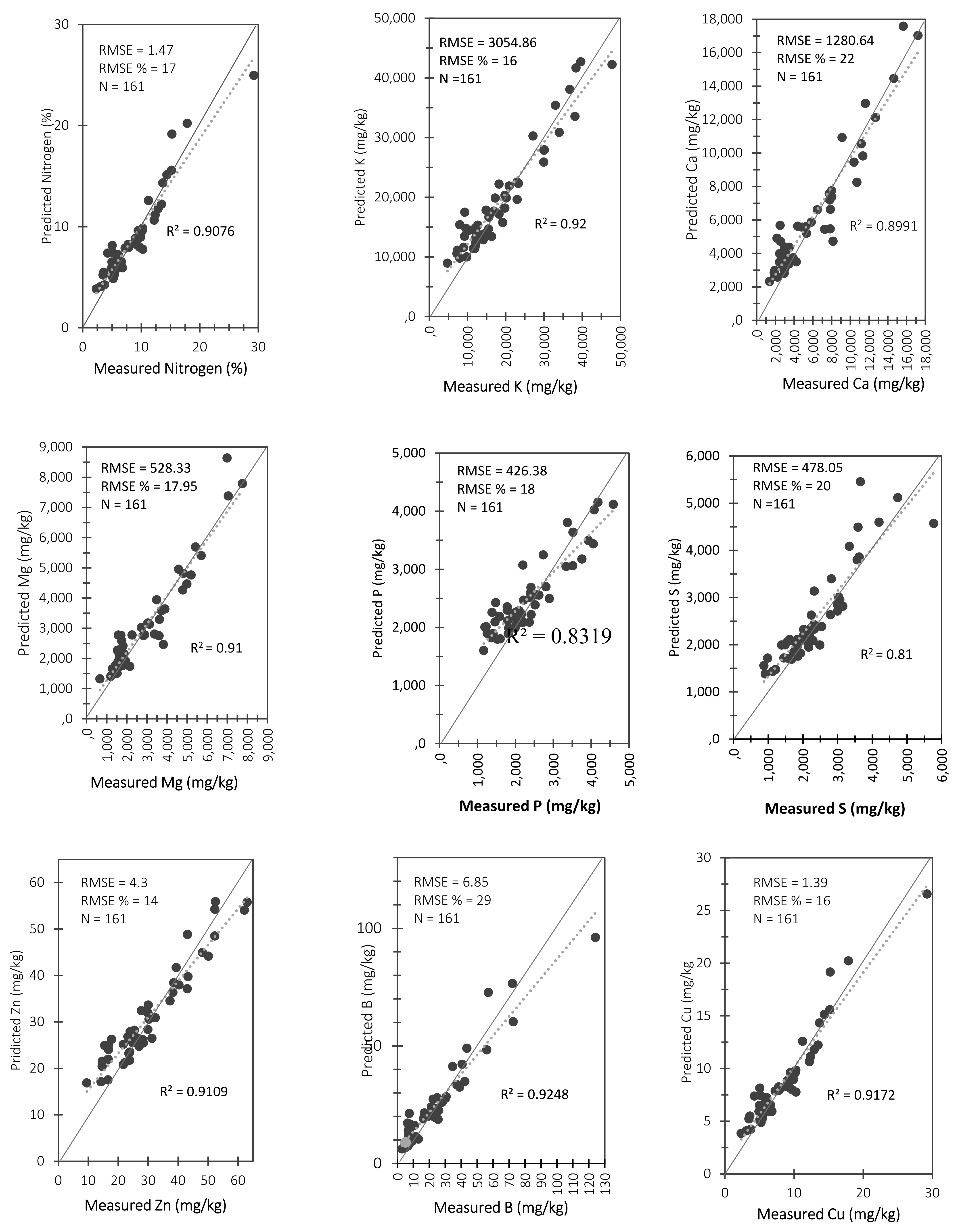
This study has shown the utility of the RF model using S-2 in estimating concentrations of N, K, Ca, Mg, P, S, Cu, Zn and B. The technique yielded high coefficients of determination ranging between 0.75 and 0.98. The technique also exhibited low RMSE % for most nutrients except for magnesium (38%), boron (43%) and calcium (30%) which emerged as difficult to detect by using the RF model and S-2. The usefulness of RF regression and remotely sensed images is demonstrated by its ability to estimate sugarcane leaf nitrogen levels from Hyperion images [104]. Multiple studies have demonstrated that RF models often perform remarkably well in different fields of scientific research including the estimation of nitrogen content [115,116,117,
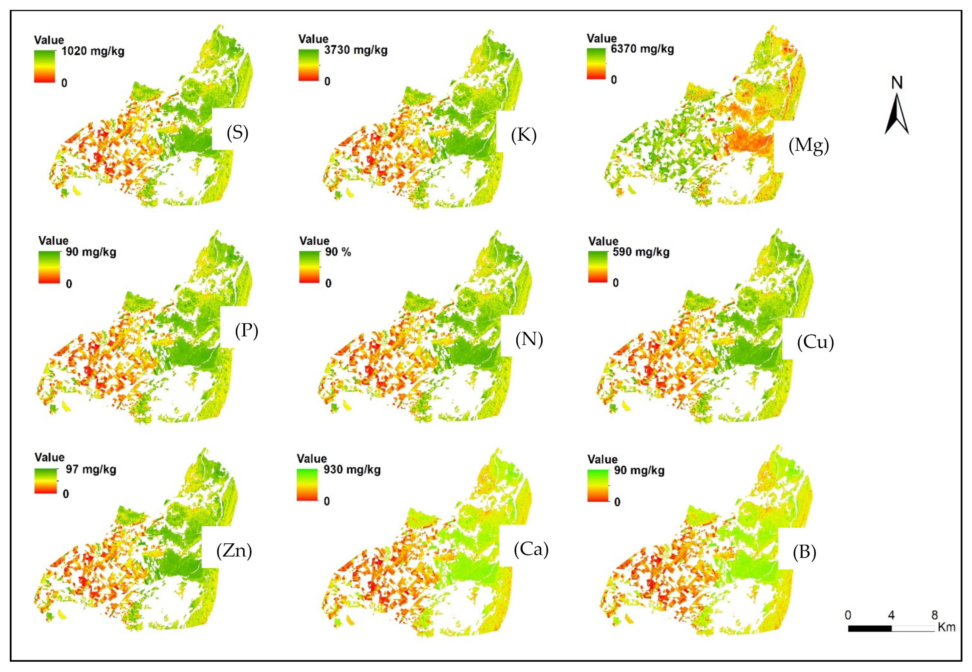
118]. In this study, fusing vegetation indices in the NIR spectral region and NIR-based vegetation indices (NDVI) with RF proved to be a suitable approach for estimating the studied nutrients. RF also proved to be suitable in relation to NDVI, REP1 and band 7 in developing a relationship between nutrient variations and land use land cover types (Figure 4) except for magnesium, which exhibited high concentrations in sugarcane farms where the land use land cover-nutrient effect variation was consistent. This is attributed to the antagonistic effects of (Ca and Mg) and K in sugarcane, where soils with high Ca and Mg can lower leaf K and vice versa.

4.2. Crops and Vegetation Nutrients Seasonal Estimations

Most nutrients exhibited significant relationships (R2 < 0.7) between measured and estimated concentrations across seasons and plant types with few that showed a weak relationship (R2 > 0.5), i.e., calcium, magnesium, phosphorus and boron). This implies that S-2 has the potential in estimating concentrations of selected chemical elements across the seasons and plant types. Generally, with the R2 accuracies in estimating foliar nutrient concentrations, there were no significant differences within nutrients from crops and vegetation between the summer and winter seasons.
Similar findings by Gama, et al. [119] confirmed a weak relationship between leaf reflectance and concentrations of phosphorus, potassium and calcium. Poor estimations of magnesium, copper and sulphur in summer were observed which implies difficulties in estimating such nutrients in a wet season. Magnesium, copper and sulphur are micronutrients that are highly affected by the processes of reduction and oxidation (redox) in concert with the shifting of water levels which determines their seasonal concentration levels in wetland soils and water. Their poor detection in this study could therefore be explained by the seasonal variations in the amount of available water which regulates the redox processes thereby and their concentration levels in soil, water different plant systems [120,121,122]. For instance, a related study [121] also concluded that seasonally occurring processes such as redox and seasonal shifts in water abundance regulate the type and amount of trace elements that are available in the water.
Moreover, high the poor performance revealed by the model’s high RMSE % suggesting across the seasons was also observed in calcium, magnesium, phosphorus and boron in wetland vegetation. Season-specific analyses showed that dry season models performed better than their wet season counterparts, as shown by their respective coefficient determinants of 0.87 in winter and 0.86 (Table 4 and Table 5). This might be attributed to the higher reflectance in the visible spectrum (bands 2, 4 and 4) in the dry season compared to the wet season. Plants are generally less green in dry seasons due to lower moisture content and less chlorophyll which leads to lower energy absorption and greater reflection. Contrary to these observations, however, Ramoelo, et al. [123]; Cho, et al. [124] and Skidmore, et al. [125] found models such as RF to perform better in the wet season compared to the dry season.

4.3. Implications of Remote Sensing on Wetland Plant Nutrients

Over the past years, several studies [126,127] have used remote sensing and chemical analyses in estimating foliar nutrient concentrations in plants. However, these studies mostly concentrated on seasonal estimations of nitrogen in grasses. This study has attempted to build on these initiatives by broadening the application of these techniques to the estimation of different nutrients. This initiative is helpful because it offers opportunities for enhanced understanding of vegetation health which has been previously regarded as a complex research area [128]. Although limited in geographical reach, our findings show that S-2 imagery could be a significant additional source of valuable information on seasonal variations in plant nutrient content.
This study has demonstrated that RF using S-2 can be useful for monitoring and estimating various plant nutrient quantities and the quality of floodplain vegetation. S-2 images yielded significant relationships between nutrient content in the NIR spectral region and NIR-based vegetation indices (NDVI). S-2 also provided an opportunity to seasonally characterize the studied nutrients. The findings of this study present a great opportunity and technique for mapping and monitoring nutrient enrichment in wetlands beyond the characterization of plant macronutrients (NPK) across both crops and natural vegetation species. This is a step towards a time-efficient and affordable technique for mapping and monitoring wetlands from local to regional scales based on S-2’s optimal spatial resolution and swath widths.
A method of performing chemical analysis in plants in the laboratory is spatially limited for many reasons. Our approach returned high coefficients of determination for most of the nutrients in crops and vegetation. By implication, remotely sensed data make up for shortcomings of the traditional methods with the advantages of real-time and rapid observations. As a result, this technique would be a useful alternative for estimating plant health conditions and nutritional status under different environmental settings.

5. Conclusions

This study demonstrated immense potentials for Sentinel-2 data to be used for estimating leaf nitrogen, potassium, calcium, magnesium, phosphorus, sulphur, zinc, boron and copper concentrations. Different vegetation indices and bands including the red edge position, NDVI and band 2 can be important in estimating different nutrients across the seasons even though foliar estimation using Sentinel-2 did not show a strong relationship in estimating leaf magnesium, copper and sulphur in a wet season. The major conclusion of this work is that the RF model was able to provide estimated nutrients with reasonable accuracies. The study, therefore, recommends that researchers elsewhere can use the methodology provided in this article as a tool in assessing and monitoring the quality of crops/vegetation in floodplain wetlands and the use of at least two scenes (satellite images) per season to achieve representative estimates over these periods. Considering that there is no consensus with regards to the performance of different machine learning techniques in characterising foliar chemical elements such as leaf nitrogen, potassium, calcium, magnesium, phosphorus, sulphur, zinc, boron and copper, future studies need to compare and assess their performance.

Author Contributions

Literature search, M.D.; figures, M.D. and M.S.; study design, M.D.; data collection, M.D. and G.C.; data analysis, M.D., M.S. and T.D.; data interpretation, M.D. and M.S.; writing, M.D. and G.C.; co-supervised, G.C.; provided guidance to the PhD study, G.C. and E.A.; guidance on the literature searches, G.C.; guidance of the study design, G.C., M.S. and T.D.; guidance and participation in results interpretation, G.C., M.S. and T.D.; supervision, G.C. and E.A.; guidance on the conceptualization of the manuscript, G.C. and E.A. All authors have read and agreed to the published version of the manuscript.

Funding

The Department of Higher Education, Science and Technology funded the study, while the Agricultural Research Council funded the analysis of plant samples.

Institutional Review Board Statement

Not applicable.

Informed Consent Statement

Not applicable.

Data Availability Statement

The data belongs to Witwatersrand University and will be kept by the authors. The data will be availed upon request for research purposes only, and the disclosure shall include the following: the title of the research or paper to be used for the stated data; the details of the organization and the supervisory body or persons concerned; the assurance that the research would not yield any commercial benefit. Our contacts are detailed in this paper to request the data.

Acknowledgments

The authors would like to thank local communities and Isimangaliso Wetland Park for allowing us to access their land during field investigation. We are also grateful to the Agricultural Research Council laboratory for analyzing our plant samples.

Conflicts of Interest

The authors declare no conflict of interest. There was no position for the funders in the study design; data collection, publication or interpretation; the writing of the manuscript or the decision to report the results of the study.

References

  1. Driver, A.; Sink, K.J.; Nel, J.L.; Holness, S.; Van Niekerk, L.; Daniels, F.; Jonas, Z.; Majiedt, P.A.; Harris, L.; Maze, K. National Biodiversity Assessment 2011: An Assessment of South Africa’s Biodiversity and Ecosystems; SANBI: Pretoria, South Africa, 2012. [Google Scholar]
  2. Kotze, D.; Marneweck, G.; Batchelor, A.; Lindley, D.; Collins, N. WET-EcoServices: A Technique for Rapidly Assessing Ecosystem Services Supplied by Wetlands; SANBI: Pretoria, South Africa, 2009. [Google Scholar]
  3. Steven, D.D.; Lowrance, R. Agricultural conservation practices and wetland ecosystem services in the wetland-rich Piedmont-Coastal Plain region. Ecol. Appl. 2011, 21, S3–S17. [Google Scholar] [CrossRef]
  4. IPCC. Intergovernmental Panel on Climate Change (IPCC); Fifth Assessment Report, Synthesis for Policy Makers; IPCC: Geneva, Switzerland, 2014. [Google Scholar]
  5. Renaud, F.G.; Sudmeier-Rieux, K.; Estrella, M. The Role of Ecosystems in Disaster Risk Reduction; United Nations University Press: Tokyo, Japan, 2013. [Google Scholar]
  6. Gardner, R.C.; Barchiesi, S.; Beltrame, C.; Finlayson, C.M.; Galewski, T.; Harrison, I.; Paganini, M.; Perennou, C.; Pritchard, D.E.; Rosenqvist, A.; et al. State of the World’s Wetlands and Their Services to People: A Compilation of Recent Analyses; Ramsar Convention Secretariat: Gland, Switzerland, 2015; p. 19. [Google Scholar]
  7. Davidson, N.; Fluet-Chouinard, E.; Finlayson, C. Global extent and distribution of wetlands: Trends and issues. Mar. Freshw. Res. 2018, 69, 620–627. [Google Scholar] [CrossRef] [Green Version]
  8. Houghton, R.A.; Hackler, J.L.; Lawrence, K.T. The US carbon budget: Contributions from land-use change. Science 1999, 285, 574–578. [Google Scholar] [CrossRef] [PubMed]
  9. Dai, A. Increasing drought under global warming in observations and models. Nat. Clim. Chang. 2013, 3, 52–58. [Google Scholar] [CrossRef]
  10. Nyirenda, R. Gendered Access to Wetland Gardens (Dimba) in Northern Malawi. Master’s Thesis, West Virginia University, Morgantown, WV, USA, 2020. [Google Scholar]
  11. Msusa, H. Sustainable utilization of wetlands for food security: A case study of the Simulemba traditional Authority in the Kasungu District of Malawi. J. Dev. Sustain. Agric. 2011, 6, 86–100. [Google Scholar]
  12. Nyamadzawo, G.; Wuta, M.; Nyamangara, J.; Nyamugafata, P.; Chirinda, N. Optimizing dambo (seasonal wetland) cultivation for climate change adaptation and sustainable crop production in the smallholder farming areas of Zimbabwe. Int. J. Agric. Sustain. 2015, 13, 23–39. [Google Scholar] [CrossRef]
  13. Zhu, Y.; Qu, Y.; Liu, S.; Chen, S. A reflectance spectra model for copper-stressed leaves: Advances in the PROSPECT model through addition of the specific absorption coefficients of the copper ion. Int. J. Remote Sens. 2014, 35, 1356–1373. [Google Scholar] [CrossRef]
  14. Verkleij, J.A.; Golan-Goldhirsh, A.; Antosiewisz, D.M.; Schwitzguébel, J.-P.; Schröder, P. Dualities in plant tolerance to pollutants and their uptake and translocation to the upper plant parts. Environ. Exp. Bot. 2009, 67, 10–22. [Google Scholar] [CrossRef]
  15. Peralta-Videa, J.R.; Lopez, M.L.; Narayan, M.; Saupe, G.; Gardea-Torresdey, J. The biochemistry of environmental heavy metal uptake by plants: Implications for the food chain. Int. J. Biochem. Cell Biol. 2009, 41, 1665–1677. [Google Scholar] [CrossRef]
  16. Mengel, K.; Kirkby, E.A.; Mengal, K.; Appel, T.; Kosegarton, H. Principles of Plant Nutrition, 5th ed.; Kluwer Academic Publishers: Dordrecht, The Netherlands, 2001. [Google Scholar]
  17. White, P.; Brown, P. Plant nutrition for sustainable development and global health. Ann. Bot. 2010, 105, 1073–1080. [Google Scholar] [CrossRef] [Green Version]
  18. Kanke, Y.; Raun, W.; Solie, J.; Stone, M.; Taylor, R. Red edge as a potential index for detecting differences in plant nitrogen status in winter wheat. J. Plant Nutr. 2012, 35, 1526–1541. [Google Scholar] [CrossRef]
  19. Clevers, J.G.; Gitelson, A.A. Remote estimation of crop and grass chlorophyll and nitrogen content using red-edge bands on Sentinel-2 and-3. Int. J. Appl. Earth Obs. Geoinf. 2013, 23, 344–351. [Google Scholar] [CrossRef]
  20. Özyiğit, Y.; Bilgen, M. Use of spectral reflectance values for determining nitrogen, phosphorus, and potassium contents of rangeland plants. J. Agric. Sci. Technol. 2013, 15, 1537–1545. [Google Scholar]
  21. Mutanga, O.; Adam, E.; Adjorlolo, C.; Abdel-Rahman, E.M. Evaluating the robustness of models developed from field spectral data in predicting African grass foliar nitrogen concentration using WorldView-2 image as an independent test dataset. Int. J. Appl. Earth Obs. Geoinf. 2015, 34, 178–187. [Google Scholar] [CrossRef]
  22. Adjorlolo, C.; Mutanga, O.; Cho, M.A. Estimation of canopy nitrogen concentration across C3 and C4 grasslands using WorldView-2 multispectral data. IEEE J. Sel. Top. Appl. Earth Obs. Remote Sens. 2014, 7, 4385–4392. [Google Scholar] [CrossRef]
  23. Ramoelo, A.; Cho, M.A. Explaining leaf nitrogen distribution in a semi-arid environment predicted on Sentinel-2 imagery using a field spectroscopy derived model. Remote Sens. 2018, 10, 269. [Google Scholar] [CrossRef] [Green Version]
  24. Mutanga, O.; Adam, E.; Cho, M.A. High density biomass estimation for wetland vegetation using WorldView-2 imagery and random forest regression algorithm. Int. J. Appl. Earth Obs. Geoinf. 2012, 18, 399–406. [Google Scholar] [CrossRef]
  25. Li, F.; Wang, L.; Liu, J.; Wang, Y.; Chang, Q. Evaluation of leaf N concentration in winter wheat based on discrete wavelet transform analysis. Remote Sens. 2019, 11, 1331. [Google Scholar] [CrossRef] [Green Version]
  26. Delloye, C.; Weiss, M.; Defourny, P. Retrieval of the canopy chlorophyll content from Sentinel-2 spectral bands to estimate nitrogen uptake in intensive winter wheat cropping systems. Remote Sens. Environ. 2018, 216, 245–261. [Google Scholar] [CrossRef]
  27. Ye, X.; Abe, S.; Zhang, S. Estimation and mapping of nitrogen content in apple trees at leaf and canopy levels using hyperspectral imaging. Precis. Agric. 2020, 21, 198–225. [Google Scholar] [CrossRef]
  28. Mahajan, G.; Pandey, R.; Sahoo, R.; Gupta, V.; Datta, S.; Kumar, D. Monitoring nitrogen, phosphorus and sulphur in hybrid rice (Oryza sativa L.) using hyperspectral remote sensing. Precis. Agric. 2017, 18, 736–761. [Google Scholar] [CrossRef]
  29. Özyiğit, Y.; Bilgen, M. Estimation of Nitrogen Levels by Remote Sensing Method in Alfalfa (Medicago sativa L.). Tarim Ve Doga Derg. 2018, 21, 902. [Google Scholar]
  30. Siqueira, R.; Longchamps, L.; Dahal, S.; Khosla, R. Use of fluorescence sensing to detect nitrogen and potassium variability in maize. Remote Sens. 2020, 12, 1752. [Google Scholar] [CrossRef]
  31. Zengeya, F.M.; Mutanga, O.; Murwira, A. Linking remotely sensed forage quality estimates from WorldView-2 multispectral data with cattle distribution in a savanna landscape. Int. J. Appl. Earth Obs. Geoinf. 2013, 21, 513–524. [Google Scholar] [CrossRef]
  32. Li, W.; Dou, Z.; Cui, L.; Wang, R.; Zhao, Z.; Cui, S.; Lei, Y.; Li, J.; Zhao, X.; Zhai, X. Suitability of hyperspectral data for monitoring nitrogen and phosphorus content in constructed wetlands. Remote Sens. Lett. 2020, 11, 495–504. [Google Scholar] [CrossRef]
  33. George, R.; Padalia, H.; Sinha, S.; Kumar, A.S. Evaluating sensitivity of hyperspectral indices for estimating mangrove chlorophyll in Middle Andaman Island, India. Environ. Monit. Assess. 2019, 191, 1–14. [Google Scholar] [CrossRef]
  34. Luo, J.; Ma, R.; Feng, H.; Li, X. Estimating the total nitrogen concentration of reed canopy with hyperspectral measurements considering a non-uniform vertical nitrogen distribution. Remote Sens. 2016, 8, 789. [Google Scholar] [CrossRef] [Green Version]
  35. Van Asselen, S.; Verburg, P.H.; Vermaat, J.E.; Janse, J.H. Drivers of wetland conversion: A global meta-analysis. PLoS ONE 2013, 8, 81292. [Google Scholar] [CrossRef] [PubMed] [Green Version]
  36. Ramoelo, A.; Cho, M.A.; Mathieu, R.; Madonsela, S.; Van De Kerchove, R.; Kaszta, Z.; Wolff, E. Monitoring grass nutrients and biomass as indicators of rangeland quality and quantity using random forest modelling and WorldView-2 data. Int. J. Appl. Earth Obs. Geoinf. 2015, 43, 43–54. [Google Scholar] [CrossRef]
  37. Barker, A.V.; Pilbeam, D.J. Handbook of Plant Nutrition; CRC Press: Boca Raton, FL, USA, 2015. [Google Scholar]
  38. Chhabra, A.; Manjunath, K.; Panigrahy, S. Non-point source pollution in Indian agriculture: Estimation of nitrogen losses from rice crop using remote sensing and GIS. Int. J. Appl. Earth Obs. Geoinf. 2010, 12, 190–200. [Google Scholar] [CrossRef]
  39. Gilbertson, J.K.; Kemp, J.; Van Niekerk, A. Effect of pan-sharpening multi-temporal Landsat 8 imagery for crop type differentiation using different classification techniques. Comput. Electron. Agric. 2017, 134, 151–159. [Google Scholar] [CrossRef] [Green Version]
  40. Lee, T.-M.; Yeh, H.-C. Applying remote sensing techniques to monitor shifting wetland vegetation: A case study of Danshui River estuary mangrove communities, Taiwan. Ecol. Eng. 2009, 35, 487–496. [Google Scholar] [CrossRef]
  41. Held, A.; Ticehurst, C.; Lymburner, L.; Williams, N. High resolution mapping of tropical mangrove ecosystems using hyperspectral and radar remote sensing. Int. J. Remote Sens. 2003, 24, 2739–2759. [Google Scholar] [CrossRef]
  42. Wood, A.; Dixon, A.; McCartney, M. People-centred wetland management. In Wetland Management and Sustainable Livelihoods in Africa; Routledge: Oxon, UK, 2013; pp. 23–64. [Google Scholar]
  43. Ollis, D.; Snaddon, K.; Job, N.; Mbona, N. Classification System for Wetlands and Other Aquatic Ecosystems in South Africa; SANBI: Pretoria, South Africa, 2013. [Google Scholar]
  44. Fennessy, M.; Mack, J.; Rokosch, A.; Knapp, M.; Micacchion, M. Biogeochemical and Hydrological Investigations of Natural and Mitigation Wetlands; Ohio EPA Technical Report WET/2004-5; Ohio EPA: Columbus, OH, USA, 2004. [Google Scholar]
  45. Dube, T.; Mutanga, O.; Ismail, R. Quantifying aboveground biomass in African environments: A review of the trade-offs between sensor estimation accuracy and costs. Trop. Ecol. 2016, 57, 393–405. [Google Scholar]
  46. Sibanda, M.; Mutanga, O.; Rouget, M. Examining the potential of Sentinel-2 MSI spectral resolution in quantifying above ground biomass across different fertilizer treatments. ISPRS J. Photogramm. Remote Sens. 2015, 110, 55–65. [Google Scholar] [CrossRef]
  47. Otunga, C.; Odindi, J.; Mutanga, O.; Adjorlolo, C. Evaluating the potential of the red edge channel for C3 (Festuca spp.) grass discrimination using Sentinel-2 and Rapid Eye satellite image data. Geocarto Int. 2019, 34, 1123–1143. [Google Scholar] [CrossRef]
  48. Chemura, A.; Mutanga, O.; Odindi, J.; Kutywayo, D. Mapping spatial variability of foliar nitrogen in coffee (Coffea arabica L.) plantations with multispectral Sentinel-2 MSI data. ISPRS J. Photogramm. Remote Sens. 2018, 138, 1–11. [Google Scholar] [CrossRef]
  49. Clevers, J.G.; Kooistra, L.; van den Brande, M.M. Using Sentinel-2 Data for Retrieving LAI and Leaf and Canopy Chlorophyll Content of a Potato Crop. Remote Sens. 2017, 9, 405. [Google Scholar] [CrossRef] [Green Version]
  50. Gao, J.; Liu, J.; Liang, T.; Hou, M.; Ge, J.; Feng, Q.; Wu, C.; Li, W. Mapping the Forage Nitrogen-Phosphorus Ratio Based on Sentinel-2 MSI Data and a Random Forest Algorithm in an Alpine Grassland Ecosystem of the Tibetan Plateau. Remote Sens. 2020, 12, 2929. [Google Scholar] [CrossRef]
  51. Frampton, W.J.; Dash, J.; Watmough, G.; Milton, E.J. Evaluating the capabilities of Sentinel-2 for quantitative estimation of biophysical variables in vegetation. ISPRS J. Photogramm. Remote Sens. 2013, 82, 83–92. [Google Scholar] [CrossRef] [Green Version]
  52. Hernández-Clemente, R.; Hornero, A.; Mottus, M.; Penuelas, J.; González-Dugo, V.; Jiménez, J.; Suárez, L.; Alonso, L.; Zarco-Tejada, P.J. Early diagnosis of vegetation health from high-resolution hyperspectral and thermal imagery: Lessons learned from empirical relationships and radiative transfer modelling. Curr. For. Rep. 2019, 5, 169–183. [Google Scholar] [CrossRef] [Green Version]
  53. Pham, T.D.; Yokoya, N.; Bui, D.T.; Yoshino, K.; Friess, D.A. Remote sensing approaches for monitoring mangrove species, structure, and biomass: Opportunities and challenges. Remote Sens. 2019, 11, 230. [Google Scholar] [CrossRef] [Green Version]
  54. Wu, L.; Zhu, X.; Lawes, R.; Dunkerley, D.; Zhang, H. Comparison of machine learning algorithms for classification of LiDAR points for characterization of canola canopy structure. Int. J. Remote Sens. 2019, 40, 5973–5991. [Google Scholar] [CrossRef]
  55. Wolanin, A.; Camps-Valls, G.; Gómez-Chova, L.; Mateo-García, G.; van der Tol, C.; Zhang, Y.; Guanter, L. Estimating crop primary productivity with Sentinel-2 and Landsat 8 using machine learning methods trained with radiative transfer simulations. Remote Sens. Environ. 2019, 225, 441–457. [Google Scholar] [CrossRef]
  56. Prado Osco, L.; Marques Ramos, A.P.; Roberto Pereira, D.; Moriya, É.A.S.; Nobuhiro Imai, N.; Takashi Matsubara, E.; Estrabis, N.; de Souza, M.; Marcato Junior, J.; Gonçalves, W.N. Predicting Canopy Nitrogen Content in Citrus-Trees Using Random Forest Algorithm Associated to Spectral Vegetation Indices from UAV-Imagery. Remote Sens. 2019, 11, 2925. [Google Scholar] [CrossRef] [Green Version]
  57. Liang, L.; Di, L.; Huang, T.; Wang, J.; Lin, L.; Wang, L.; Yang, M. Estimation of leaf nitrogen content in wheat using new hyperspectral indices and a random forest regression algorithm. Remote Sens. 2018, 10, 1940. [Google Scholar] [CrossRef] [Green Version]
  58. Polikar, R. Ensemble based systems in decision making. IEEE Circuits Syst. Mag. 2006, 6, 21–45. [Google Scholar] [CrossRef]
  59. Breiman, L. Random forests. Mach. Learn. 2001, 45, 5–32. [Google Scholar] [CrossRef] [Green Version]
  60. Burai, P.; Deák, B.; Valkó, O.; Tomor, T. Classification of herbaceous vegetation using airborne hyperspectral imagery. Remote Sens. 2015, 7, 2046–2066. [Google Scholar] [CrossRef] [Green Version]
  61. Doktor, D.; Lausch, A.; Spengler, D.; Thurner, M. Extraction of plant physiological status from hyperspectral signatures using machine learning methods. Remote Sens. 2014, 6, 12247–12274. [Google Scholar] [CrossRef] [Green Version]
  62. Ghimire, B.; Rogan, J.; Miller, J. Contextual land-cover classification: Incorporating spatial dependence in land-cover classification models using random forests and the Getis statistic. Remote Sens. Lett. 2010, 1, 45–54. [Google Scholar] [CrossRef] [Green Version]
  63. Grimm, R.; Behrens, T.; Märker, M.; Elsenbeer, H. Soil organic carbon concentrations and stocks on Barro Colorado Island—Digital soil mapping using Random Forests analysis. Geoderma 2008, 146, 102–113. [Google Scholar] [CrossRef]
  64. Prasad, A.M.; Iverson, L.R.; Liaw, A. Newer classification and regression tree techniques: Bagging and random forests for ecological prediction. Ecosystems 2006, 9, 181–199. [Google Scholar] [CrossRef]
  65. Adelabu, S.; Mutanga, O.; Adam, E.; Cho, M.A. Exploiting machine learning algorithms for tree species classification in a semiarid woodland using RapidEye image. J. Appl. Remote Sens. 2013, 7, 073480. [Google Scholar] [CrossRef]
  66. Garden, S. Wetland Geomorphology and Floodplain Dynamics on the Hydrologically Variable Mfolozi River, KwaZulu-Natal, South Africa. Ph.D. Thesis, University of KwaZulu-Natal, Durban, South Africa, 2008. [Google Scholar]
  67. Morgenthal, T.; Kellner, K.; Van Rensburg, L.; Newby, T.; Van der Merwe, J. Vegetation and habitat types of the Umkhanyakude Node. S. Afr. J. Bot. 2006, 72, 1–10. [Google Scholar] [CrossRef] [Green Version]
  68. Schulze, R.E. South African Atlas of Agrohydrology and Climatology; Water Research Commission: Pretoria, South Africa, 1997. [Google Scholar]
  69. Öztürk, Ö.; Ceyhan, E.; Önder, M.; Harmankaya, M.; Hamurcu, M.; Gezgin, S. Micronutrient contents in leaves of sunflower cultivars grown with different boron doses. Helia 2010, 33, 215–220. [Google Scholar] [CrossRef] [Green Version]
  70. Gardner, R.C.; Finlayson, M. Global Wetland Outlook: State of the World’s Wetlands and their Services to People; Ramsar Convention: Gland, Switzerland, 2018. [Google Scholar]
  71. Muller-Wilm, U.; Louis, J.; Richter, R.; Gascon, F.; Niezette, M. Sentinel-2 level 2A prototype processor: Architecture, algorithms and first results. In Proceedings of the ESA Living Planet Symposium, Edinburgh, UK, 9–13 September 2013; pp. 9–13. [Google Scholar]
  72. Farahmand, N.; Sadeghi, V. Estimating Soil Salinity in the Dried Lake Bed of Urmia Lake Using Optical Sentinel-2 Images and Nonlinear Regression Models. J. Indian Soc. Remote Sens. 2020, 48, 1–13. [Google Scholar] [CrossRef]
  73. Van Passel, J.; De Keersmaecker, W.; Somers, B. Monitoring woody cover dynamics in tropical dry forest ecosystems using sentinel-2 satellite imagery. Remote Sens. 2020, 12, 1276. [Google Scholar] [CrossRef] [Green Version]
  74. Jordan, C.F. Derivation of leaf-area index from quality of light on the forest floor. Ecology 1969, 50, 663–666. [Google Scholar] [CrossRef]
  75. Gitelson, A.; Merzlyak, M.N. Spectral reflectance changes associated with autumn senescence of Aesculus hippocastanum L. and Acer platanoides L. leaves. Spectral features and relation to chlorophyll estimation. J. Plant Physiol. 1994, 143, 286–292. [Google Scholar] [CrossRef]
  76. Barnes, E.; Clarke, T.; Richards, S.; Colaizzi, P.; Haberland, J.; Kostrzewski, M.; Waller, P.; Choi, C.; Riley, E.; Thompson, T. Coincident detection of crop water stress, nitrogen status and canopy density using ground based multispectral data. In Proceedings of the Fifth International Conference on Precision Agriculture, Bloomington, MN, USA, 16–19 July 2000. [Google Scholar]
  77. Gitelson, A.A.; Gritz, Y.; Merzlyak, M.N. Relationships between leaf chlorophyll content and spectral reflectance and algorithms for non-destructive chlorophyll assessment in higher plant leaves. J. Plant Physiol. 2003, 160, 271–282. [Google Scholar] [CrossRef]
  78. Gitelson, A.A.; Keydan, G.P.; Merzlyak, M.N. Three-band model for noninvasive estimation of chlorophyll, carotenoids, and anthocyanin contents in higher plant leaves. Geophys. Res. Lett. 2006, 33. [Google Scholar] [CrossRef] [Green Version]
  79. Dash, J.; Curran, P.J.; Tallis, M.J.; Llewellyn, G.M.; Taylor, G.; Snoeij, P. Validating the MERIS Terrestrial Chlorophyll Index (MTCI) with ground chlorophyll content data at MERIS spatial resolution. Remote Sens. 2010, 31, 5513–5532. [Google Scholar] [CrossRef] [Green Version]
  80. Xue, J.; Su, B. Significant Remote Sensing Vegetation Indices: A Review of Developments and Applications. J. Sens. 2017, 2017, 1353691. [Google Scholar] [CrossRef] [Green Version]
  81. Aklilu Tesfaye, A.; Gessesse Awoke, B. Evaluation of the saturation property of vegetation indices derived from sentinel-2 in mixed crop-forest ecosystem. Spat. Inf. Res. 2021, 29, 109–121. [Google Scholar] [CrossRef]
  82. Zhao, D.; Huang, L.; Li, J.; Qi, J. A comparative analysis of broadband and narrowband derived vegetation indices in predicting LAI and CCD of a cotton canopy. ISPRS J. Photogramm. Remote Sens. 2007, 62, 25–33. [Google Scholar] [CrossRef]
  83. Mahajan, G.R.; Das, B.; Murgaokar, D.; Herrmann, I.; Berger, K.; Sahoo, R.N.; Patel, K.; Desai, A.; Morajkar, S.; Kulkarni, R.M. Monitoring the Foliar Nutrients Status of Mango Using Spectroscopy-Based Spectral Indices and PLSR-Combined Machine Learning Models. Remote Sens. 2021, 13, 641. [Google Scholar] [CrossRef]
  84. Pullanagari, R.R.; Kereszturi, G.; Yule, I. Integrating airborne hyperspectral, topographic, and soil data for estimating pasture quality using recursive feature elimination with random forest regression. Remote Sens. 2018, 10, 1117. [Google Scholar] [CrossRef] [Green Version]
  85. Yang, H.; Li, F.; Wang, W.; Yu, K. Estimating Above-Ground Biomass of Potato Using Random Forest and Optimized Hyperspectral Indices. Remote Sens. 2021, 13, 2339. [Google Scholar]
  86. Thenkabail, P.S.; Lyon, J.G.; Huete, A. Hyperspectral Remote Sensing of Vegetation; CRC Press: Boca Raton, FL, USA, 2011. [Google Scholar]
  87. Ishwaran, H. The effect of splitting on random forests. Mach. Learn. 2015, 99, 75–118. [Google Scholar] [CrossRef]
  88. Ok, A.O.; Akar, O.; Gungor, O. Evaluation of random forest method for agricultural crop classification. Eur. J. Remote Sens. 2012, 45, 421–432. [Google Scholar] [CrossRef]
  89. Sandri, M.; Zuccolotto, P. Variable selection using random forests. In Data Analysis, Classification and the Forward Search; Springer: Berlin, Germany, 2006; pp. 263–270. [Google Scholar]
  90. Hapfelmeier, A.; Ulm, K. A new variable selection approach using random forests. Comput. Stat. Data Anal. 2013, 60, 50–69. [Google Scholar] [CrossRef]
  91. Grömping, U. Variable importance assessment in regression: Linear regression versus random forest. Am. Stat. 2009, 63, 308–319. [Google Scholar] [CrossRef]
  92. Otgonbayar, M.; Atzberger, C.; Chambers, J.; Damdinsuren, A. Mapping pasture biomass in Mongolia using Partial Least Squares, Random Forest regression and Landsat 8 imagery. Int. J. Remote Sens. 2019, 40, 3204–3226. [Google Scholar] [CrossRef]
  93. Shcherbakov, M.V.; Brebels, A.; Shcherbakova, N.L.; Tyukov, A.P.; Janovsky, T.A.; Kamaev, V.A.e. A survey of forecast error measures. World Appl. Sci. J. 2013, 24, 171–176. [Google Scholar]
  94. Richter, K.; Hank, T.B.; Mauser, W.; Atzberger, C. Derivation of biophysical variables from Earth observation data: Validation and statistical measures. J. Appl. Remote Sens. 2012, 6, 063557. [Google Scholar] [CrossRef]
  95. Karl, J.W.; McCord, S.E.; Hadley, B.C. A comparison of cover calculation techniques for relating point-intercept vegetation sampling to remote sensing imagery. Ecol. Indic. 2017, 73, 156–165. [Google Scholar] [CrossRef] [Green Version]
  96. Chen, J.; Zhu, W.; Tian, Y.Q.; Yu, Q.; Zheng, Y.; Huang, L. Remote estimation of colored dissolved organic matter and chlorophyll-a in Lake Huron using Sentinel-2 measurements. J. Appl. Remote Sens. 2017, 11, 036007. [Google Scholar] [CrossRef]
  97. Osco, L.P.; Ramos, A.P.M.; Faita Pinheiro, M.M.; Moriya, É.A.S.; Imai, N.N.; Estrabis, N.; Ianczyk, F.; Araújo, F.F.d.; Liesenberg, V.; Jorge, L.A.d.C. A Machine Learning Framework to Predict Nutrient Content in Valencia-Orange Leaf Hyperspectral Measurements. Remote Sens. 2020, 12, 906. [Google Scholar] [CrossRef] [Green Version]
  98. Shah, S.H.; Angel, Y.; Houborg, R.; Ali, S.; McCabe, M.F. A random forest machine learning approach for the retrieval of leaf chlorophyll content in wheat. Remote Sens. 2019, 11, 920. [Google Scholar] [CrossRef] [Green Version]
  99. Huang, S.; Miao, Y.; Yuan, F.; Gnyp, M.L.; Yao, Y.; Cao, Q.; Wang, H.; Lenz-Wiedemann, V.I.; Bareth, G. Potential of RapidEye and WorldView-2 satellite data for improving rice nitrogen status monitoring at different growth stages. Remote Sens. 2017, 9, 227. [Google Scholar] [CrossRef] [Green Version]
  100. Kalacska, M.; Lalonde, M.; Moore, T. Estimation of foliar chlorophyll and nitrogen content in an ombrotrophic bog from hyperspectral data: Scaling from leaf to image. Remote Sens. Environ. 2015, 169, 270–279. [Google Scholar] [CrossRef]
  101. Munyati, C.; Balzter, H.; Economon, E. Correlating Sentinel-2 MSI-derived vegetation indices with in-situ reflectance and tissue macronutrients in savannah grass. Int. J. Remote Sens. 2020, 41, 3820–3844. [Google Scholar] [CrossRef]
  102. Lepine, L.C.; Ollinger, S.V.; Ouimette, A.P.; Martin, M.E. Examining spectral reflectance features related to foliar nitrogen in forests: Implications for broad-scale nitrogen mapping. Remote Sens. Environ. 2016, 173, 174–186. [Google Scholar] [CrossRef]
  103. Wang, Z.; Wang, T.; Darvishzadeh, R.; Skidmore, A.K.; Jones, S.; Suarez, L.; Woodgate, W.; Heiden, U.; Heurich, M.; Hearne, J. Vegetation indices for mapping canopy foliar nitrogen in a mixed temperate forest. Remote Sens. 2016, 8, 491. [Google Scholar] [CrossRef] [Green Version]
  104. Abdel-Rahman, E.M.; Ahmed, F.B.; Ismail, R. Random forest regression and spectral band selection for estimating sugarcane leaf nitrogen concentration using EO-1 Hyperion hyperspectral data. Int. J. Remote Sens. 2013, 34, 712–728. [Google Scholar] [CrossRef]
  105. Ramoelo, A.; Cho, M.; Mathieu, R.; Skidmore, A.K. Potential of Sentinel-2 spectral configuration to assess rangeland quality. J. Appl. Remote Sens. 2015, 9, 094096. [Google Scholar] [CrossRef] [Green Version]
  106. Raper, T.; Varco, J. Canopy-scale wavelength and vegetative index sensitivities to cotton growth parameters and nitrogen status. Precis. Agric. 2015, 16, 62–76. [Google Scholar] [CrossRef] [Green Version]
  107. Schlemmer, M.; Gitelson, A.; Schepers, J.; Ferguson, R.; Peng, Y.; Shanahan, J.; Rundquist, D. Remote estimation of nitrogen and chlorophyll contents in maize at leaf and canopy levels. Int. J. Appl. Earth Obs. Geoinf. 2013, 25, 47–54. [Google Scholar] [CrossRef] [Green Version]
  108. Marschner, H. Mineral Nutrition of Higher Plants, 2nd ed.; Academic Press: Cambirdge, MA, USA, 1995. [Google Scholar]
  109. Ferwerda, J.G.; Skidmore, A.K. Can nutrient status of four woody plant species be predicted using field spectrometry? ISPRS J. Photogramm. Remote Sens. 2007, 62, 406–414. [Google Scholar] [CrossRef]
  110. Mutanga, O.; Skidmore, A.K.; Prins, H. Predicting in situ pasture quality in the Kruger National Park, South Africa, using continuum-removed absorption features. Remote Sens. Environ. 2004, 89, 393–408. [Google Scholar] [CrossRef]
  111. Pinheiro Lisboa, I.; Melo Damian, J.; Roberto Cherubin, M.; Silva Barros, P.P.; Ricardo Fiorio, P.; Cerri, C.C.; Eduardo Pellegrino Cerri, C. Prediction of sugarcane yield based on NDVI and concentration of leaf-tissue nutrients in fields managed with straw removal. Agronomy 2018, 8, 196. [Google Scholar] [CrossRef] [Green Version]
  112. Van Deventer, H.; Cho, M.A. Assessing leaf spectral properties of Phragmites australis impacted by acid mine drainage. S. Afr. J. Sci. 2014, 110, 1–12. [Google Scholar] [CrossRef] [Green Version]
  113. Martinez, N.; Sharp, J.; Kuhne, W.; Johnson, T.; Stafford, C.; Duff, M. Assessing the use of reflectance spectroscopy in determining CsCl stress in the model species Arabidopsis thaliana. Int. J. Remote Sens. 2015, 36, 5887–5915. [Google Scholar] [CrossRef]
  114. Rathod, P.H.; Brackhage, C.; Van der Meer, F.D.; Müller, I.; Noomen, M.F.; Rossiter, D.G.; Dudel, G.E. Spectral changes in the leaves of barley plant due to phytoremediation of metals—Results from a pot study. Eur. J. Remote Sens. 2015, 48, 283–302. [Google Scholar] [CrossRef]
  115. Freeman, E.A.; Moisen, G.G.; Frescino, T.S. Evaluating effectiveness of down-sampling for stratified designs and unbalanced prevalence in Random Forest models of tree species distributions in Nevada. Ecol. Model. 2012, 233, 1–10. [Google Scholar] [CrossRef]
  116. Freeman, E.A.; Moisen, G.G.; Coulston, J.W.; Wilson, B.T. Random forests and stochastic gradient boosting for predicting tree canopy cover: Comparing tuning processes and model performance. Can. J. For. Res. 2016, 46, 323–339. [Google Scholar] [CrossRef] [Green Version]
  117. Cutler, D.R.; Edwards Jr, T.C.; Beard, K.H.; Cutler, A.; Hess, K.T.; Gibson, J.; Lawler, J.J. Random forests for classification in ecology. Ecology 2007, 88, 2783–2792. [Google Scholar] [CrossRef] [PubMed]
  118. Verikas, A.; Gelzinis, A.; Bacauskiene, M. Mining data with random forests: A survey and results of new tests. Pattern Recognit. 2011, 44, 330–349. [Google Scholar] [CrossRef]
  119. Gama, M.J.; Cho, M.A.; Chirwa, P.; Masemola, C. Estimating mineral content of indigenous browse species using laboratory spectroscopy and Sentinel-2 imagery. Int. J. Appl. Earth Obs. Geoinf. 2019, 75, 141–150. [Google Scholar] [CrossRef]
  120. Lu, Q.; Bai, J.; Gao, Z.; Wang, J.; Zhao, Q. Effects of Water Level and Salinity on Total Sulfur Contents in Salt Marsh Soils of the Yellow River Delta, China. Wetlands 2016, 36, 137–143. [Google Scholar] [CrossRef]
  121. Olivie-Lauquet, G.; Gruau, G.; Dia, A.; Riou, C.; Jaffrezic, A.; Henin, O. Release of trace elements in wetlands: Role of seasonal variability. Water Res. 2001, 35, 943–952. [Google Scholar] [CrossRef]
  122. Ribeiro, B.T.; Nascimento, D.C.; Curi, N.; Guilherme, L.R.G.; Costa, E.T.d.S.; Lopes, G.; Carneiro, J.P. Assessment of Trace Element Contents in Soils and Water from Cerrado Wetlands, Triângulo Mineiro Region. Rev. Bras. de Ciência do Solo 2019, 43, 0180059. [Google Scholar] [CrossRef] [Green Version]
  123. Ramoelo, A.; Skidmore, A.K.; Cho, M.A.; Schlerf, M.; Mathieu, R.; Heitkönig, I.M. Regional estimation of savanna grass nitrogen using the red-edge band of the spaceborne RapidEye sensor. Int. J. Appl. Earth Obs. Geoinf. 2012, 19, 151–162. [Google Scholar] [CrossRef]
  124. Cho, M.A.; Ramoelo, A.; Debba, P.; Mutanga, O.; Mathieu, R.; Van Deventer, H.; Ndlovu, N. Assessing the effects of subtropical forest fragmentation on leaf nitrogen distribution using remote sensing data. Landsc. Ecol. 2013, 28, 1479–1491. [Google Scholar] [CrossRef]
  125. Skidmore, A.K.; Ferwerda, J.G.; Mutanga, O.; Van Wieren, S.E.; Peel, M.; Grant, R.C.; Prins, H.H.; Balcik, F.B.; Venus, V. Forage quality of savannas—Simultaneously mapping foliar protein and polyphenols for trees and grass using hyperspectral imagery. Remote Sens. Environ. 2010, 114, 64–72. [Google Scholar] [CrossRef]
  126. Oliveira, L.F.R.d.; Santana, R.C.; Oliveira, M.L.R.d. Nondestructive estimation of leaf nutrient concentrations in Eucalyptus plantations. Cerne 2019, 25, 184–194. [Google Scholar] [CrossRef]
  127. Mahajan, G.; Sahoo, R.; Pandey, R.; Gupta, V.; Kumar, D. Using hyperspectral remote sensing techniques to monitor nitrogen, phosphorus, sulphur and potassium in wheat (Triticum aestivum L.). Precis. Agric. 2014, 15, 499–522. [Google Scholar] [CrossRef]
  128. Mutanga, O.; Dube, T.; Ahmed, F. Progress in remote sensing: Vegetation monitoring in South Africa. S. Afr. Geogr. J. 2016, 98, 461–471. [Google Scholar] [CrossRef]
Figure 1. Geographic location of the study area in KwaZulu Natal province, South Africa.
Remotesensing 13 04249 g001
Figure 2. The flow chart summarises the overall methods for the study.
Remotesensing 13 04249 g002
Figure 3. Accuracies derived in estimating N, K, Ca, Mg, P, S, Zn, B, Cu concentrations using testing data sets. Dotted lines in the graph illustrate the linear regression line.
Remotesensing 13 04249 g003
Figure 4. Importance of variables that were used to estimate N, Ca, K, Mg, P, Cu, Zn, B and, S by using S-2 MIS derived vegetation indices data. NB *, %IncMSE is Mean decrease accuracy, IncNodePurity is mean decrease Gini, REP; 1, 2 and 3 is red edge position 1, 2 and 3, chlorophyll green (Cl. Green), simple ratio (SR; 1, 2 and 3), MTCI.1 is MERIS Terrestrial Chlorophyll Index 1, NDVI is normalised difference vegetation index, nDVI (nDVI_Bγi_ Bγj) is modified normalised vegetation difference index and sR (sR_Bγi_ Bγj) _ is modified sample ratio where Bγi_ Bγj are any Sentinel 2 MSI bands excluding bands 1, 9 and 10.
Remotesensing 13 04249 g004aRemotesensing 13 04249 g004b
Figure 5. Spatial distribution of nutrients: S, K, Mg, Cu, N, P, Zn, Ca and B.
Remotesensing 13 04249 g005
Table 1. Temporal sequencing, identity details, cloud cover percentages of Sentinel-2 images that were used and field samples by scene ID.
SeasonImage Acquisition DateSample Collection DateScene IDCloud Cover (%)No of Samples
Wet27 March 201712 March 2017S2A_MSIL1C_20170327T074231_N0204_R049_T36JVP0.476
Dry18 July 201722 July 2017S2A_MSIL1C_20170718T075211_N0205_R092_T36JVP085
Table 2. Vegetation indices used in this study. The Sentinel-2 band IDs are used in the formulas (as per Section 2.2.1).
NameEquationReferences
Normalised Difference Vegetation Index (NDVI)(NIR − R)/(NIR + R)[74]
Simple Ratio (SR)NIR/R[74]
Simple Ratio 1 (SR1)Re2/R[74]
Simple Ratio 2 (SR2)Re3/R[74]
Simple Ratio 3 (SR3)R3/R2[75]
Red Edge Position 1 (REP1)(R1 − R)/2[19,76]
Red Edge 2 Position 2 (REP2)(R2 − R1)/2[19,76]
Red Edge 3 Position 3 (REP3)(R3 − R2)/2[19,76]
Chlorophyll Red Edge (CIred-edge)(Re3/R2) − 1[19]
Chlorophyll Green (CI green)(R3/green) − 1[77,78]
The MERIS Terrestrial Chlorophyll Index (MTCI 1)(NIR − R2/R705)/(R2 − R)[79]
Modified NDVI (nDVI)(Bγi) − (Bγj)/(Bγi) + (Bγj)[46]
Modified Simple Ratio (sR)(Bγi)/(Bγj)[46]
NB: Bγi and Bγj are different Sentinel 2 MSI spectral bands.
Table 3. Experiments were performed using S-2 MSI data to estimate macro and micronutrient concentrations in crops and wetland vegetation.
AnalysisData ManipulationSpectral Data Used
1Separate plant functional types and seasonsBands and vegetation band indices separately
2Pooled based on plant functional types and both seasonsBands and vegetation indices separately
3Pooled based on nutrient types across all plant typesVegetation indices
Table 4. Dry and wet season nutrient concentration estimation accuracies for crops.
Raw Spectral BandsVegetation Indices
PeriodElementMSRVar Expl %R2RMSERMSE %MSRVar Expl %R2RMSERMSE %
SummerN%0.36620.640.65320.20890.970.5123
K (mg/kg)34,589,753.00650.7511,898.333410,233,470.00860.967357.8328
Ca (mg/kg)66,890,049.00290.735889.755226,130,783.00570.953924.5612
Mg (mg/kg)5,751,843.00350.743452.00303,335,425.06890.981969.8232
P (mg/kg)157,738.20660.74768.7831786,589.96900.94689.5326
S (mg/kg)218,191.40540.691172.1734176,031.10850.95966.1229
Zn (mg/kg)43.85760.610.973230.84870.968.5626
B (mg/kg)484.50520.5923.1342325.52650.8813.9829
Cu(mg/kg)16.56540.7112.363212.99660.945.8626
WinterN%0.33730.560.69330.15830.710.8227
K (mg/kg)20,789,123.00710.716512.123214,545,775.00820.8739,794.2027
Ca (mg/kg)2,189,691.00640.722289.59361,876,120.00870.811582.8228
Mg (mg/kg)307,861.79600.61989.2832259,985.90860.83672.5825
P (mg/kg)92,876.18680.59548.963169,886.90840.79391.8622
S (mg/kg)258,951.21530.58681.5930200,100.10750.79398.3020
Zn (mg/kg)28.80660.629.993220.74730.755.9924
B (mg/kg)43.94690.5610.933730.96800.855.1630
Cu (mg/kg)2.99700.673.98301.28820.762.9025
Explanation: MSR = mean squared residual, Var Expl % = variance explained percentage, R2 = R-squared, RMSE % = root mean square error (percentage).
Table 5. Dry and wet season nutrient concentration variations accuracies for wetland vegetation.
Raw Spectral BandsVegetation Indices
PeriodElementMSRVar Expl %R2RMSERMSE %MSRVar Expl %R2RMSERMSE %
SummerN%0.16740.650.88290.145685690.820.57523125
K (mg/kg)18,186,459.00510.513849.734013,815,824670.882989.12520
Ca (mg/kg)59,128,582.00490.621789.77294,812,124550.851500.13227
Mg (mg/kg)698,784.20540.571123.9035598,798.9640.93980.01230
P (mg/kg)558,987.10510.53594.4829498,689.99660.73512.35424
S (mg/kg)8,289,574.00130.361289.2033791,210.01100.27981.01231
Zn (mg/kg)41.87530.6419.492837.39468.90.8014.058122
B (mg/kg)98.58580.5714.553889.7865600.8910.0135
Cu(mg/kg)4.18690.639.28302.001087670.836.1235124
WinterN%0.19570.661.00290.12986870.890.70123
K (mg/kg)42,894,179.00630.616188.082938,215,694800.975010.5622
Ca (mg/kg)9,989,987.00530.561684.49298,614,811730.981498.35625
Mg (mg/kg)4,958,737.005269.00991.88384,015,420590.98865.211330
P (mg/kg)29,879,879.00390.63497.99242,132,142450.90390.1215
S (mg/kg)69,688.79670.67798.393265,211.32880.92701.12426
Zn (mg/kg)32.99680.567.942625.096890.945.99887923
B (mg/kg)199.93620.686.8829150.32135680.954.9879425
Cu (mg/kg)7.02530.563.97284.325612740.951.978921
Table 6. Comparisons of nutrient estimation accuracies (RMSE %) between the summer and winter seasons in crops and vegetation, respectively.
RMSE%
PlantsStatisticsSummer Winter
CropsRank Sum13852
p-value (α = 0.05)0.001
VegetationRank Sum189.269.2
p-value (α = 0.05)0.012
Table 7. Seasonal nutrient estimation accuracies for crops and vegetation.
Plant TypeNutrientMSRVar ExplRMSE
%R2RMSE%
Wetland
vegetation
N0.18624369.970.940.4818
K65,985,61584.820.837235.7829
Ca1,869,48681.950.882610.230
Mg247,612.9880.830.752166.4838
P202,121.777.850.781231.2529
S3,981,612.239.440.84310.4112
Zn11.5877688.220.884.0114
B119.01278.480.799.1243
Cu0.884489.20.882.1229
CropsN0.1879988.510.940.30112
K13,131,61390.120.962911.5914
Ca15,532,85359.750.951433.2120
Mg149,81468.70.95511.5113
P99,539.785.620.95221.111
S14,912.3870.95221.7212
Zn18.1345290.040.962.5112
B123.8974581.420.986.0125
Cu4.176552388.610.881.718
Table 8. Descriptive statistics for R2 values and RMSE% for vegetation and crop types using pooled data.
Accuracy UnitStatisticsVegetationCrops
R2Mean0.840.94
Maximum0.880.98
Minimum0.750.88
Median0.840.95
St deviation0.060.027
p-value 0.02
RMSE %Mean1527
Maximum2543
Minimum1112
Median2929
St deviation1329
p-value 0.001
Publisher’s Note: MDPI stays neutral with regard to jurisdictional claims in published maps and institutional affiliations.

