Chaos Based Frequency Modulation for Joint Monostatic and Bistatic Radar-Communication Systems

Abstract

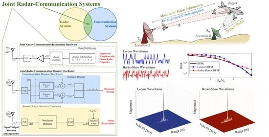
In this article, we propose the utilization of chaos-based frequency modulated (CBFM) waveforms for joint monostatic and bistatic radar-communication systems. Short-duration pulses generated via chaotic oscillators are used for wideband radar imaging, while information is embedded in the pulses using chaos shift keying (CSK). A self-synchronization technique for chaotic systems decodes the information at the communication receiver and reconstructs the transmitted waveform at the bistatic radar receiver. Using a nonlinear detection scheme, we show that the CBFM waveforms closely follow the theoretical bit-error rate (BER) associated with bipolar phase-shift keying (BPSK). We utilize the same nonlinear detection scheme to optimize the target detection at the bistatic radar receiver. The ambiguity function for both the monostatic and bistatic cases resembles a thumbtack ambiguity function with a pseudo-random sidelobe distribution. Furthermore, we characterize the high-resolution imaging capability of the CBFM waveforms in the presence of noise and considering a complex target.

1. Introduction

Due to an exponential increase in the utilization of communication devices and limitations on the electromagnetic spectrum, there is tremendous demand for radio frequency systems [1] to operate simultaneously without any mutual interference. In particular, radar is now sharing its allocated spectrum, while expectations are that it should perform optimally [2]. Consequently, the coexistence of communications and radar systems is necessary now more than ever.

Joint radar-communication systems (RadComm) can be realized using two main approaches [3]. The first approach is using a single platform where hardware is reduced for simultaneous functionality. For instance, a xampling-based technology is utilized for radar and communication spectrum sharing [4], where the communications and radar systems transmit at separate spectral bands to avoid interference. Multiple-input multiple-output (MIMO) radar and communication systems are proposed in [5,6]. It is noted that the functionality of these systems may be preferred by examining the environment [3,7]. A transceiver architecture along with a dual-functional radar-communication (DFRC) system using a hybrid analog-digital beamforming technique in mm waveband is proposed in [8]. With many of these proposed techniques, the complexities associated with the transmitter hardware can be reduced along with the operational and functional costs [8]. One of the major drawbacks of this approach is the mutual interference caused by each system. Additional signal processing efforts are required to mitigate the interference [9,10].

The second approach is a more efficient way in which a single transmitter is used for dual radar-communication functioning. A single waveform in which the information is embedded into the radar transmission can be used for the dual purpose of communicating and radar sensing. Much of the research is focused on designing such a dual waveform. An excellent review of historical development and current state-of-the-art on joint radar-communication systems along with modulation schemes and systems are presented in [11]. Examples of these waveforms include intrapulse basis waveforms [12], orthogonal frequency division multiplexing (OFDM) [13], linear frequency modulated waveforms [14,15], phase-modulated waveforms [16], random sequence encoding [17], embedding multiple phase-shift keying symbols onto linear frequency modulated waveforms [18], etc. An overview of dual-function radar-communications (DFRC) and various waveform schemes are noted in [19]. Many of the proposed waveforms are either radar-centric or communication-centric. They either have high sidelobes suffering high-resolution imaging capabilities, or they have high bit-error rates.

Wide bandwidth waveforms are necessary to obtain finer resolution images to classify radar targets [20]. Similarly, wideband waveforms are necessary for communication systems to transmit data at higher rates [21]. The wideband waveforms are typically generated by modulating the frequency of a long pulse for a fixed signal-to-noise ratio. Alternatively, noise-like waveforms that are inherently wideband are used for simultaneous radar and communication systems [22]. Chaotic signals are a special case of noise-like waveforms that were demonstrated to have potentials for communications [23,24,25,26,27,28,29,30,31,32,33,34], ranging [35,36] and radar systems [37,38,39,40,41] individually. However, their advantages for dual-function radar communications are not fully explored.

2. Contributions of Our Work

In this work, we explore and demonstrate the potentials of chaos for dual radar-communication functionality. To the best of the authors’ knowledge, this is the first series of experiments to combine the chaotic radars and communication systems using chaos. In particular, this will be the first work to present the joint bistatic radar-communication system using chaos. To that end, we:

• Generate a chaos-based frequency-modulated (CBFM) waveform for dual functionality. First, the chaos shift-keying approach is used to encode digital information onto the chaotic system and thereby using it as an instantaneous frequency to transmit CBFM pulses.
• Show that the proposed waveforms perform better in terms of bit-error rate and imaging capabilities than the current RadComm waveforms.
• Demonstrate that the CBFM waveform in bistatic configuration solves two issues. Firstly, reconstruct the transmitted waveform at the receiver via a direct synchronization scheme and a simple response chaotic oscillator. Secondly, to obtain the high-resolution imagery of targets.
• Illustrate the high-resolution imaging capabilities of the CBFM waveform for a monostatic radar mode.

The remainder of the paper is as follows. Section 3 will show a way to generate a CBFM waveform with digital information embedded in it. Section 4 describes the architecture to decode the information at the communication receiver. Section 5 shows a systematic procedure to reconstruct the transmitted waveform and simulate cross-ambiguity functions. Will will also characterize CBFM bistatic radar performance by simulating complex target imagery and analyze cross-ambiguity function in the presence of noise. Finally, in Section 6, we will show the high-resolution imaging capabilities of chaotic monostatic radar.

3. Generation of CBFM Waveforms for Joint Radar-Communications

An N-dimensional chaotic system is mathematically given by a set of differential equations [42] such as

$$\frac{d\mathbf{X}}{dt}=f\left(\mathbf{X}\right)$$

(1)

where f is a nonlinear function, and $\mathbf{X}$ is a vector of N-chaotic state variables. These systems are governed by control parameters that dictate the periodic, quasi-periodic and chaotic nature of the system [43]. For illustration purposes, we considered three-dimensional Lorenz [44] and Burke–Shaw [45] systems that are given in

Table 1. Nonlinear differential equations governing the Lorenz [44] and Burke–Shaw [45] dissipative chaotic systems, their control parameter values, and corresponding Lyapunov exponents.

System	Differential Equations at the Transmitter	Control Parameters	Largest Lyapunov Exponents
Lorenz	${\dot{x}}_t={\gamma }_L\left[{\sigma }_i(y_t-x_t)\right]$ ${\dot{y}}_t={\gamma }_L[x_t(\rho -z_t)-y_t]$ ${\dot{z}}_t={\gamma }_L[x_t{y}_t-{\beta }_i{z}_t]$	${\gamma }_L=2.2\times {10}^{-3}$ ${\sigma }_{(-1)}=10$,${\sigma }_{(+1)}=14$ $\rho =28$ ${\beta }_{(-1)}=\frac{8}{3}$, ${\beta }_{(+1)}=\frac{8}{3}+0.6$	${\lambda }_{(-1)}=0.8924$ ${\lambda }_{(+1)}=0.9335$
Burke–Shaw	${\dot{x}}_t={\gamma }_B[-U_i(x_t+y_t)]$ ${\dot{y}}_t={\gamma }_B[-U_i{x}_t{z}_t-y_t]$ ${\dot{z}}_t={\gamma }_B[U_i{x}_t{y}_t+V_i]$	${\gamma }_B=2.7\times {10}^{-3}$ $U_{(-1)}=10$,$U_{(+1)}=11$, $V_{(-1)}=13$,$V_{(+1)}=16$	${\lambda }_{(-1)}=2.2490$ ${\lambda }_{(+1)}=2.5159$

. Many other chaotic systems, such as Chua’s circuit (multi-scroll) [46], can yield similar results. It should be noted that the performance of the communication receiver depends on the time it takes to self-synchronize. Lorenz, Burke–Shaw, and Chua systems self-synchronize relatively faster than other oscillators such as the Rössler system. Varying time constants of chaotic systems [47] and linear methodologies such as frequency scaling [48] can improve the communication and bistatic radar performance. However, these implementations are beyond the scope of this work. Instead, the digital information is encoded using the chaos-shift keying approach, where the control parameters of the system are continuously varied in proportion to the digital information $i\left(t\right)$ [24,25,49]. Here, $i\left(t\right)$ takes on values of $-1$ and $+1$, i.e., $i\left(t\right)$, a data stream that could be thought of as a pseudo-random sequence of antipodal bits.

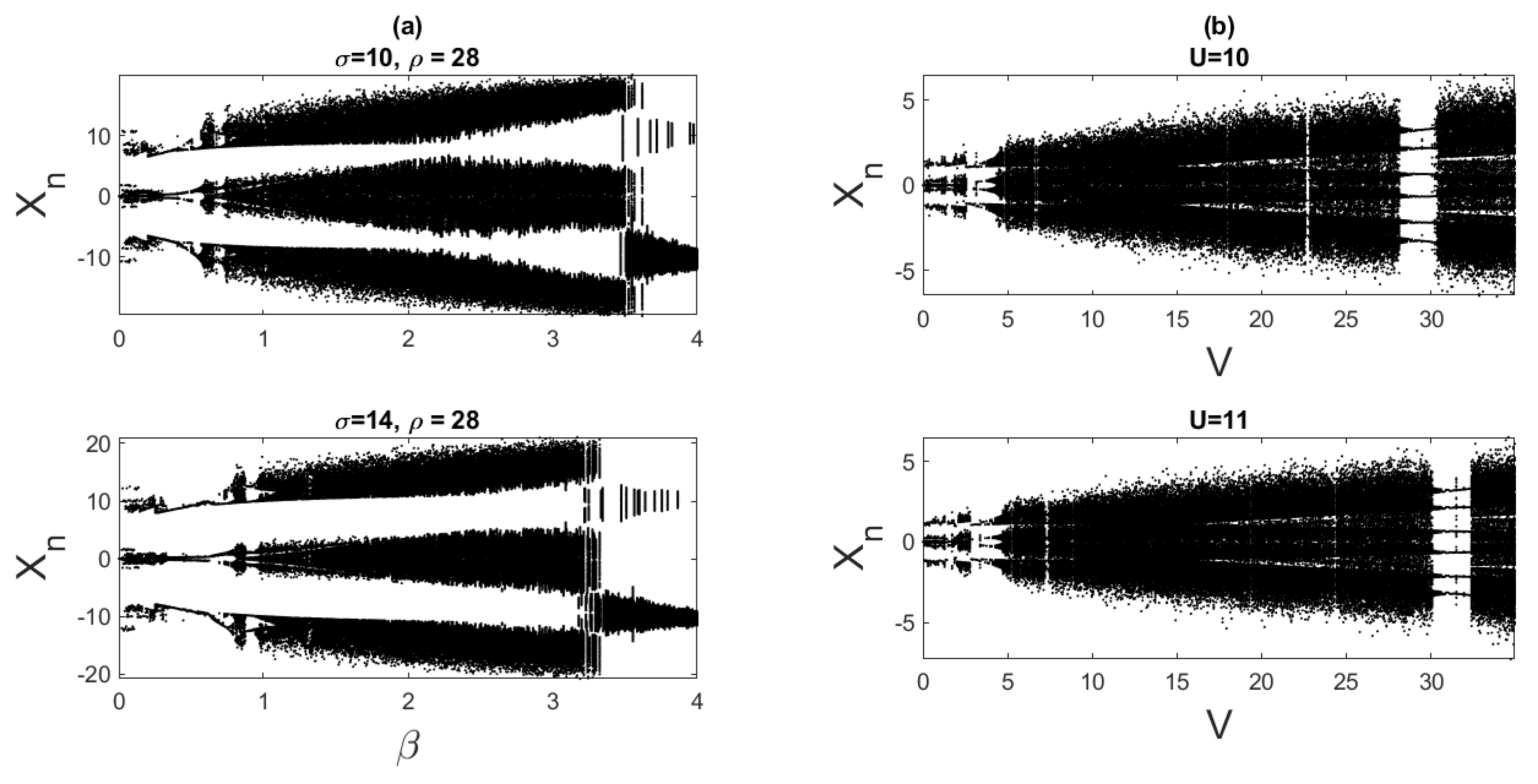
Figure 1 shows the bifurcation plot of the (a) Lorenz and (b) Burke–Shaw systems. The y-axis is the maxima of the x-state variable ($X_n$). For the Lorenz system, the bifurcation parameter is considered to be $\beta$. When $\rho =28$ and $\sigma =10$, the chaotic region is from $0.72<\beta <3.46$. Similarly, when $\rho =28$ and $\sigma =14$, the chaotic region is $0.97<\beta <3.315$. For the Burke–Shaw system, the bifurcation parameter is V. When $U=10$, the chaotic region occurs between $5<V<28$, and for $U=11$, the chaotic region is $5<V<30$. In both cases, with change in $\sigma ,\beta ,U$, and V, the dynamics of the bifurcation plot are not easily altered.

For the Lorenz system, the control parameter $\rho =28$ is constant, while the other two control parameters $\sigma$ and $\rho$ are a function of time given as

$$\begin{array}{cc}\hfill {\sigma }_i\left(t\right)& =12+2i\left(t\right)\hfill \\ \hfill {\beta }_i\left(t\right)& =\left(\frac{8}{3}+0.3\right)+0.3i\left(t\right).\hfill \end{array}$$

(2)

when a bit $-1$ is encoded, ${\sigma }_{(-1)}=10$, and ${\beta }_{(-1)}=8/3$. When a bit $+1$ is encoded, ${\sigma }_{(+1)}=14$, and ${\beta }_{(+1)}=8/3+0.6$. For the remainder of the paper, the subscripts $(-1)$ and $(+1)$ indicate that encoded bits are $-1$ and $+1$, respectively.

Similarly, for the Burke–Shaw system, the control parameters U and V are varied as

$$\begin{array}{cc}\hfill U_i\left(t\right)& =10.5+0.5i\left(t\right)\hfill \\ \hfill V_i\left(t\right)& =14.5+1.5i\left(t\right).\hfill \end{array}$$

(3)

Hence, $U_{(-1)}=10$, $V_{(-1)}=13$ and $U_{(+1)}=11$, $V_{(+1)}=16$.

The selection of the control parameters given in Equations (2) and (3) are based on the chaotic region, as shown in Figure 1. In addition to bifurcation analysis, to verify that the system is chaotic for the selected control parameters, we computed the largest Lyapunov exponent ($\lambda$) using the QR decomposition method [50]. A positive value of $\lambda$ indicates that the system quickly diverges from its original orbit with an infinitesimal change in the initial conditions, making the system chaotic. Values of the largest Lyapunov exponents ${\lambda }_{(-1)}$ and ${\lambda }_{(+1)}$ for the Lorenz and Burke–Shaw systems are summarized in Table 1. The values ${\gamma }_L$ and ${\gamma }_B$ are the time constants used to compress or dilate the chaotic system. These particular values are chosen to obtain the identical bandwidth for the Lorenz-based CBFM and Burke–Shaw-based CBFM waveforms. In all the cases, the largest Lyapunov exponent is positive, indicating that the system is always chaotic despite changing the selected control parameter values.

Note that despite changing the control parameters by a fraction of $\pm 1$ (as the function of time), the $\lambda$s are identical. An identical $\lambda$ value indicates that the characteristics of the system do not change drastically, and this can be observed from the time-series plot shown in Figure 2.

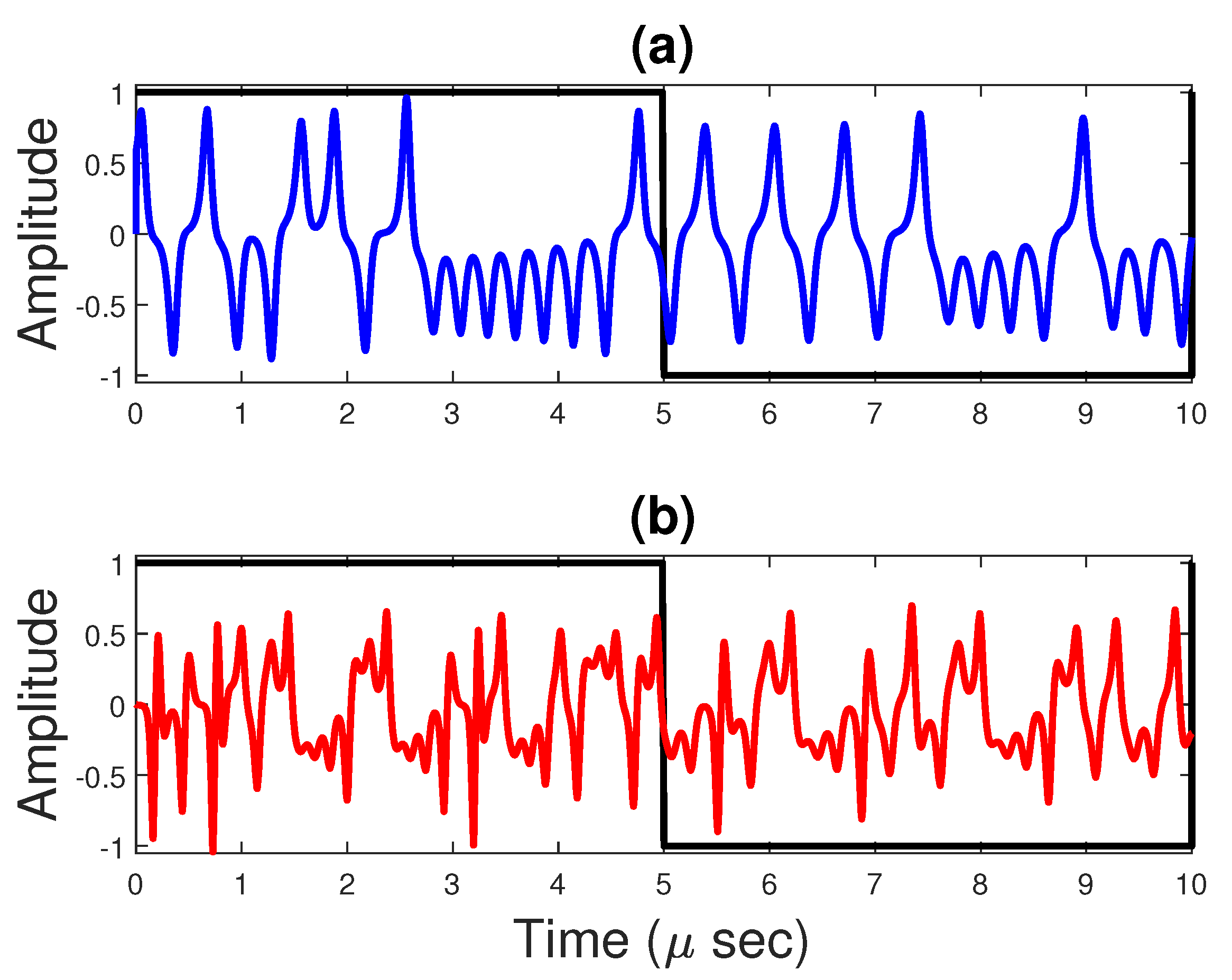
With this chaos-shift keying approach, the output of a chaotic system inherently has information encoded in it without altering the bandwidth of the chaotic signal. Figure 2 shows the normalized time series plots of $x\left(t\right)$ for both the Lorenz and Burke–Shaw chaotic systems. The systems are simulated using the Runge–Kutta fourth-order method with a sampling interval of $1ns$. Both the time series plots consist of information but without revealing what bits are encoded.

The scaled version of $x\left(t\right)$ acts as an input to the voltage-controlled oscillator (VCO). The scaling factor $\zeta$ equal to the absolute maximum value of the $x\left(t\right)$ is necessary to avoid spectral aliasing. Alternately, to reduce the additional hardware components, this scaling process can be achieved using the amplitude control approach, as shown in [51].

$$v_i\left(t\right)=\frac{x\left(t\right)}{\zeta }.$$

(4)

The above input voltage $v_i\left(t\right)$ controls the frequency oscillations of the VCO output, thus generating the CBFM waveform which, is expressed as

$$s\left(t\right)=Aexp\left(j2\pi f_{c}t+j2\pi K\underset{0}{\overset{t}{\int }}{v}_i\left(\alpha \right)d\alpha \right).$$

(5)

where $A=1$, is the amplitude to obtain a constant envelope, $f_c=300$ MHz is the carrier frequency, and K is the modulation index adjusted to obtain a bandwidth of 150 MHz. This particular bandwidth is chosen in order to obtain the range-resolution $\Delta r=\frac{c}{2\beta }=1$ m and considering the demodulation limits of the phase-locked loop. Notice that the generated FM waveform has a fractional bandwidth $\frac{\beta }{f_c}=0.5$, thereby not satisfying the narrow band criteria where the fractional bandwidth should be less than $0.1$. It should be noted that the frequencies of the chaotic systems are typically limited based on the circuitry. Unlike the work shown in [41], we modulate the chaotic signal onto the frequency carrier to generate the CBFM waveform. The spectral width of the generated CBFM waveform can be controlled using voltage-controlled oscillators to achieve the described bandwidths. Consequently, the spectrum of the CBFM waveform is independent of the circuit components of chaotic oscillators.

Figure 3 shows an illustration of the joint radar-communication system. The generated CBFM waveform transmitted from location A is used for both sensing and communications. Communication is possible via ground-to-air (communicating with aircraft) or ground-to-ground (a device on the ground). The radar sensing is possible either in monostatic mode in which the transmitter and receiver are collocated or in the bistatic mode where the transmitter and receiver are separated. Note that the communication receiver can also act as the bistatic radar receiver. The details of the communication receiver and bistatic/monostatic radar configurations are given in subsequent sections.

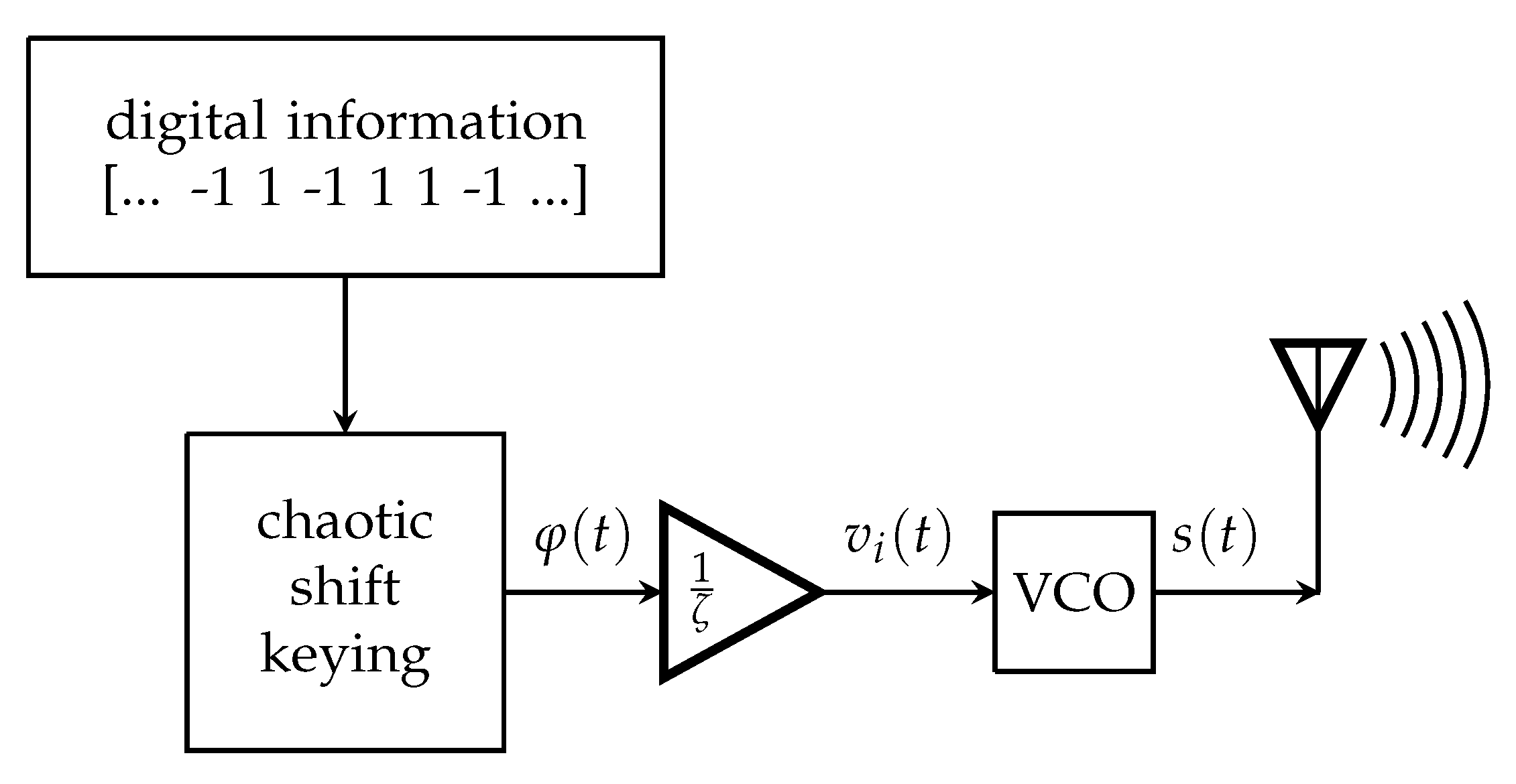
Figure 4 shows the architecture of the joint radar-communication system transmitter. Here, the digital information is encoded into the chaotic system that is further modulated on to frequency to generate the CBFM waveform. This modulation step serves several purposes. Mainly, it increases the bandwidth of the transmitted signal, which is necessary for high-resolution radar imaging. Secondly, it provides an additional security blanket without revealing what type of information is encoded. Here, the security is through obfuscation and not any standard type of encryption. Lastly, it is immune to noise up to a certain degree of freedom.

The selection of the chaotic state variable depends on the conditional Lyapunov exponent of the response oscillator (discussed in the next section). Thus, there may be some systems where state variable $x\left(t\right)$ may not serve the purpose of synchronization, but other state variables will do.

4. Communication Receiver

To decode the information, the self-synchronization scheme of chaotic systems is utilized [52,53]. Consider two identical chaotic systems: a driver and a response system (an RCO). These two systems are synchronized by driving (forcing) the response system using a chaotic signal generated from the driver. This type of synchronization is only possible if both the systems are identical in the sense that they have the same dynamical equations and control parameters. If the control parameters are mismatched, the error between the driver and response does not approach zero asymptotically. Furthermore, for a given driving function, the RCO is stable if the conditional Lyapunov exponents are negative [53].

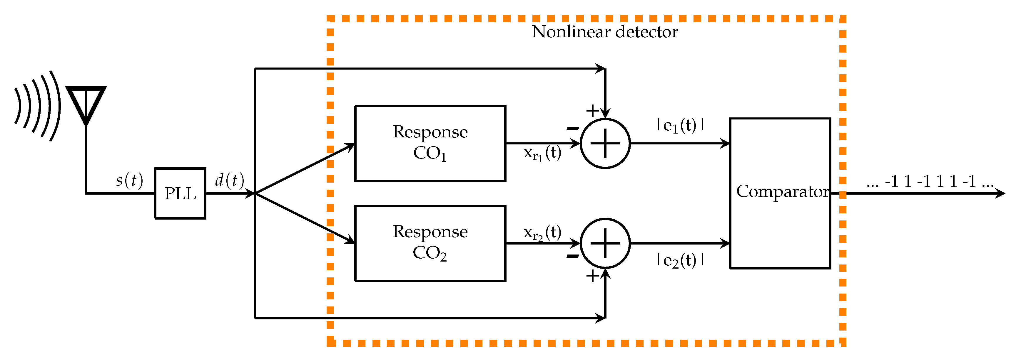
Figure 5 shows the communication receiver that consists of a phase-locked loop (PLL) and a nonlinear detector. The received CBFM waveform is driven through the PLL, which consists of an infinite impulse response lowpass Butterworth third-order filter to eliminate higher harmonics, a mixer, and a local voltage-controlled oscillator that is arbitrarily initialized. The output of PLL $p\left(t\right)$ approximates the instantaneous frequency $v_i\left(t\right)$ of the transmitted waveform, i.e., $p\left(t\right)\approx v_i\left(t\right)$ [54]. The scaled version of $p\left(t\right)$, i.e., $d\left(t\right)=\zeta p\left(t\right)$ acts as a driving function to synchronize the RCOs that are tuned to two sets of control parameters. The first RCO is tuned to the control parameters with respect to bit (−1) and the second RCO to the bit (+1). The corresponding dynamical equations of the Lorenz and Burke–Shaw RCOs are given in

Table 2. Dynamical equations for the response oscillator and its corresponding conditional-Lyapunov exponents demonstrating the stability of the response chaotic oscillators.

System	Differential Equations of RCOs		Conditional Lyapunov Exponents
Lorenz	RCO1	${\dot{x}}_{r_1}={\gamma }_L\left[10(y_{r_1}-x_{r_1})\right]$ ${\dot{y}}_{r_1}={\gamma }_L[d\left(t\right)(\rho -z_{r_1})-y_{r_1}]$ ${\dot{z}}_{r_1}={\gamma }_L\left[d\left(t\right)y_{r_1}-\frac{8}{3}{z}_{r_1}\right]$	${\lambda }_{C_1}=-1.7814$ ${\lambda }_{C_2}=-1.8862$
	RCO2	${\dot{x}}_{r_2}={\gamma }_L\left[14(y_{r_2}-x_{r_2})\right]$ ${\dot{y}}_{r_2}={\gamma }_L[d\left(t\right)(\rho -z_{r_2})-y_{r_2}]$ ${\dot{z}}_{r_2}={\gamma }_L\left[d\left(t\right)y_{r_2}-\left(\frac{8}{3}+0.6\right)z_{r_2}\right]$	${\lambda }_{C_1}=-2.1332$ ${\lambda }_{C_2}=-2.1353$
Burke–Shaw	RCO1	${\dot{x}}_{r_1}={\gamma }_B[-10(x_{r_1}+y_{r_1})]$ ${\dot{y}}_{r_1}={\gamma }_B[-10d\left(t\right)z_{r_1}-y_{r_1}]$ ${\dot{z}}_{r_1}={\gamma }_B[10d\left(t\right)y_{r_1}+13]$	${\lambda }_{C_1}=-0.4906$ ${\lambda }_{C_2}=-0.5102$
	RCO2	${\dot{x}}_{r_2}={\gamma }_B[-11(x_{r_2}+y_{r_2})]$ ${\dot{y}}_{r_2}={\gamma }_B[-11d\left(t\right)z_{r_2}-y_{r_2}]$ ${\dot{z}}_{r_2}={\gamma }_B[11d\left(t\right)y_{r_2}+16]$	${\lambda }_{C_1}=-0.4933$ ${\lambda }_{C_2}=-0.5076$

. The conditional Lyapunov exponents of RCOs for both sets of control parameters are negative, making them stable response systems.

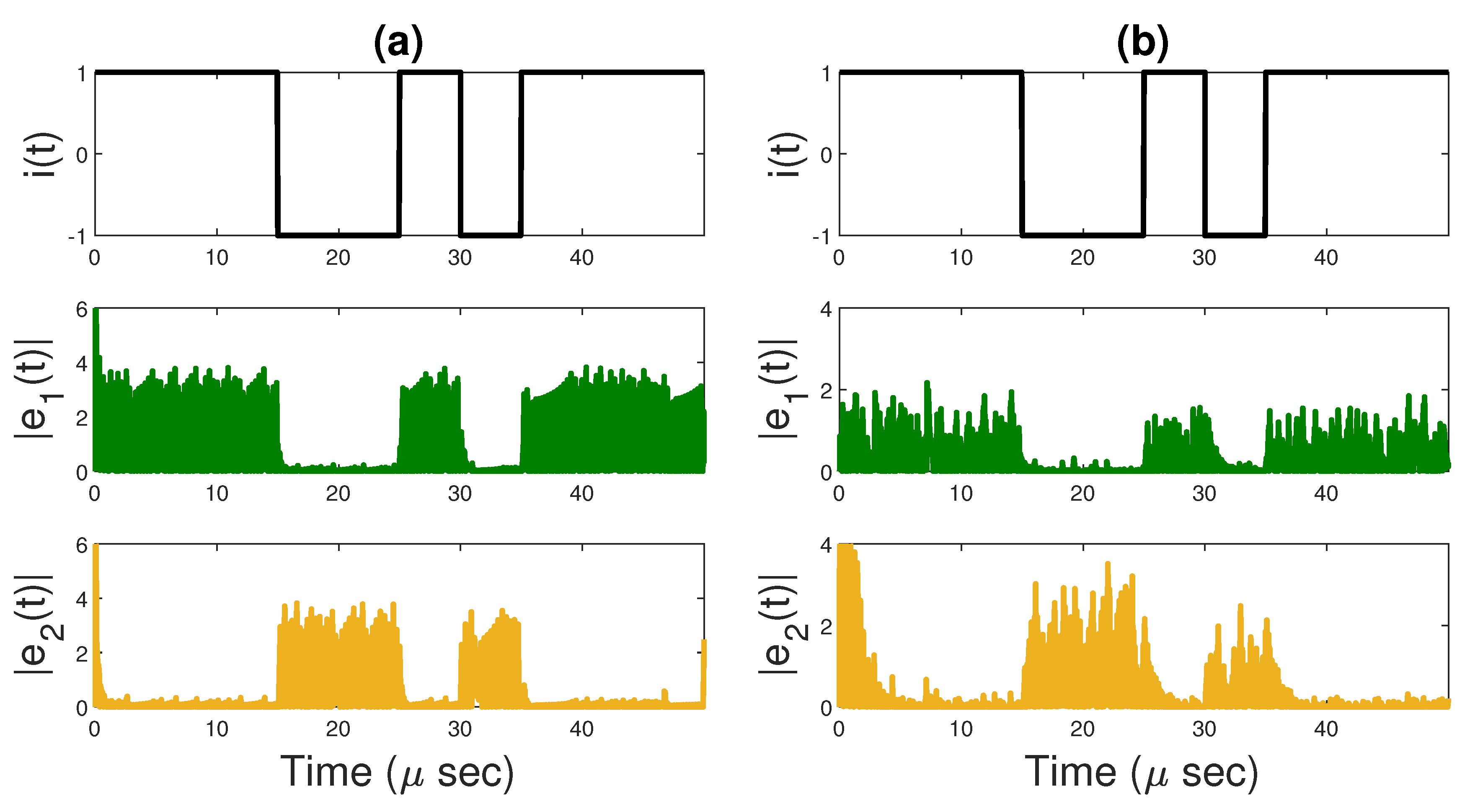
In this context, the combination of two RCOs, summers and a comparator, is called the nonlinear detector. The two RCOs will become synchronized to $d\left(t\right)$ according to the control parameters associated with the transmitted signal. When a bit (−1) is encoded, the control parameters of the Lorenz system at the transmitter are $\{10,28,8/3\}$ and hence RCO₁ will be synchronized to $d\left(t\right)$ with the error $|e_1\left(t\right)|=|d\left(t\right)-x_{r_1}\left(t\right)|$ approaching zero asymptotically. Due to parameter mismatch, RCO₂ will not be synchronized causing a significant amplitude in error $|e_2\left(t\right)|=|d\left(t\right)-x_{r_2}\left(t\right)|$. Similarly, when a bit (+1) is encoded, the control parameters of the Lorenz system at the transmitter are $\{14,28,8/3+0.6\}$. In this case, RCO₂ will synchronize with a very low error $|e_2\left(t\right)|$ while RCO₁ will be out of sync with high error amplitudes. Figure 6a shows an illustration of errors $|e_1\left(t\right)|$ and $|e_2\left(t\right)|$ when information is encoded onto the Lorenz system. Similar results can be obtained for the Burke–Shaw system, as shown in Figure 6b. For illustration purposes, we concatenated several encoded bits as a single waveform. However, considering the bistatic radar system, we considered that one CBFM waveform pulse could transmit only one bit of information. A data rate of 0.2 Mbits/s is used for our simulations.

To decode the digital information, a nonlinear detection scheme is used. The comparator is used to compare the error between RCO₁, RCO₂ and $d\left(t\right)$ to obtain $|e_1\left(t\right)|$ and $|e_2\left(t\right)|$ and decode the bits. It is mathematically expressed as Equation (6), where, $T_b=5\mathsf{\mu }$s is the duration of bit, $n=0,1,2,\dots ,N$ is the n^th bit and N is the total number of encoded bits.

$$\begin{array}{cc}\hfill \underset{n{T}_b}{\overset{(n+1)T_b}{\int }}\left|e_1\left(t\right)\right|dt& \underset{+1}{\overset{-1}{\lessgtr }}\underset{n{T}_b}{\overset{(n+1)T_b}{\int }}\left|e_2\left(t\right)\right|dt\hfill \end{array}$$

(6)

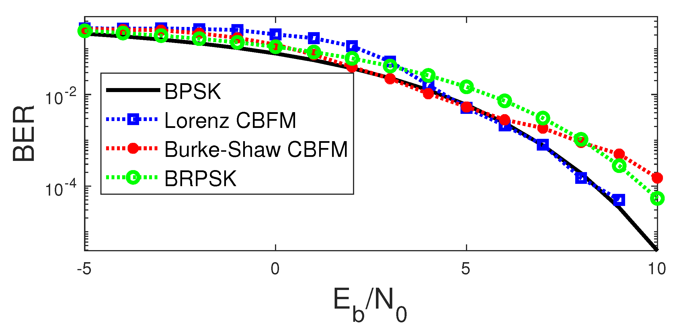
To assess the performance of a communication waveform, the bit error rate ($BER$) as the function of the ratio of energy per bit to noise spectral density ($E_b/N_0$) is used. Figure 7 shows the BER plots for the bipolar shift keying (BPSK), chaos-based FM waveforms using the Lorenz and Burke–Shaw systems. A total of 100,000 signal realizations are used to compute the BER values. For higher noise, the Lorenz CBFM yields high BER values. In contrast, the Burke–Shaw CBFM waveform performs well with BER values close to the theoretical BER values of the BPSK waveform. However, when the noise levels are less, i.e., for $E_b/N_0>4$, the BER curve of the Lorenz CBFM waveform closely follows the theoretical BER curve of the BPSK waveform. Consequently, there is a tradeoff of transmission between these two CBFM waveforms depending on the noise in communication channels.

To show the effectiveness of our proposed communications waveform, we compared our results with state-of-the-art binary reduced phase shift keying $\left(BRPSK\right)$ as presented in [14,15]. The BER of the BRPSK is given as

$$\begin{array}{c}\hfill P_b=Q\left(\sqrt{\frac{2E_{b}si{n}^2\left(\varphi \right)}{N_0}}\right)\end{array}$$

(7)

where, phases $-\varphi$ and $\varphi$ represent the binary data (two constellation points). If $\varphi ={90}^{\circ }$, the BRPSK waveform is essentially the BPSK waveform. The essence of the BRPSK waveform is to have a minor phase difference such that the constellation points have the minimum distance between them. For comparison purposes, we considered $\left|\varphi \right|={60}^{\circ }$ and simulated the BER against the $E_b/N_0$. It can be observed that the BER curves of the CBFM waveforms closely follow the BRPSK that is embedded in the traditional radar chirp waveform. In particular, for low noise, the Lorenz CBFM waveform performs better compared to the BRPSK, whereas the Burke–Shaw CBFM performs well in a high noise environment.

Typically the radar waveforms are transmitted at a very high power in the magnitudes of $1$ MW. In contrast, a typical communication waveform is transmitted in the order of KW. Therefore, the proposed communication receiver will have a significant signal-to-noise ratio compared to the traditional communication receivers. Thus, the CBFM waveforms (in particular the Lorenz CBFM waveform) are good candidates for communication systems while simultaneously offering advantages for the monostatic and bistatic radars presented in the subsequent sections.

5. Bistatic Radar Receiver Synchronization and Ambiguity Function

5.1. Synchronizing the Bistatic Radar Receiver

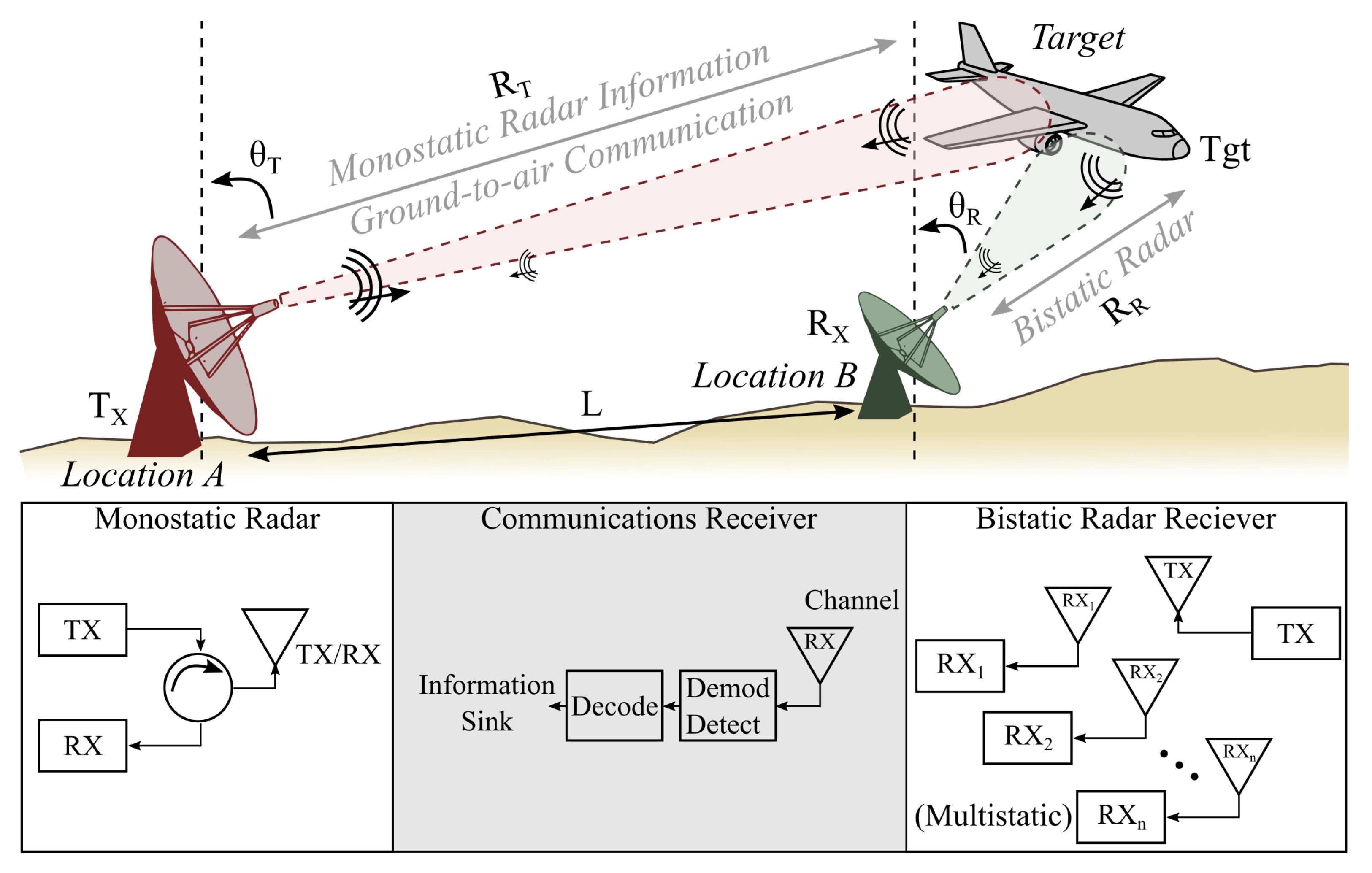
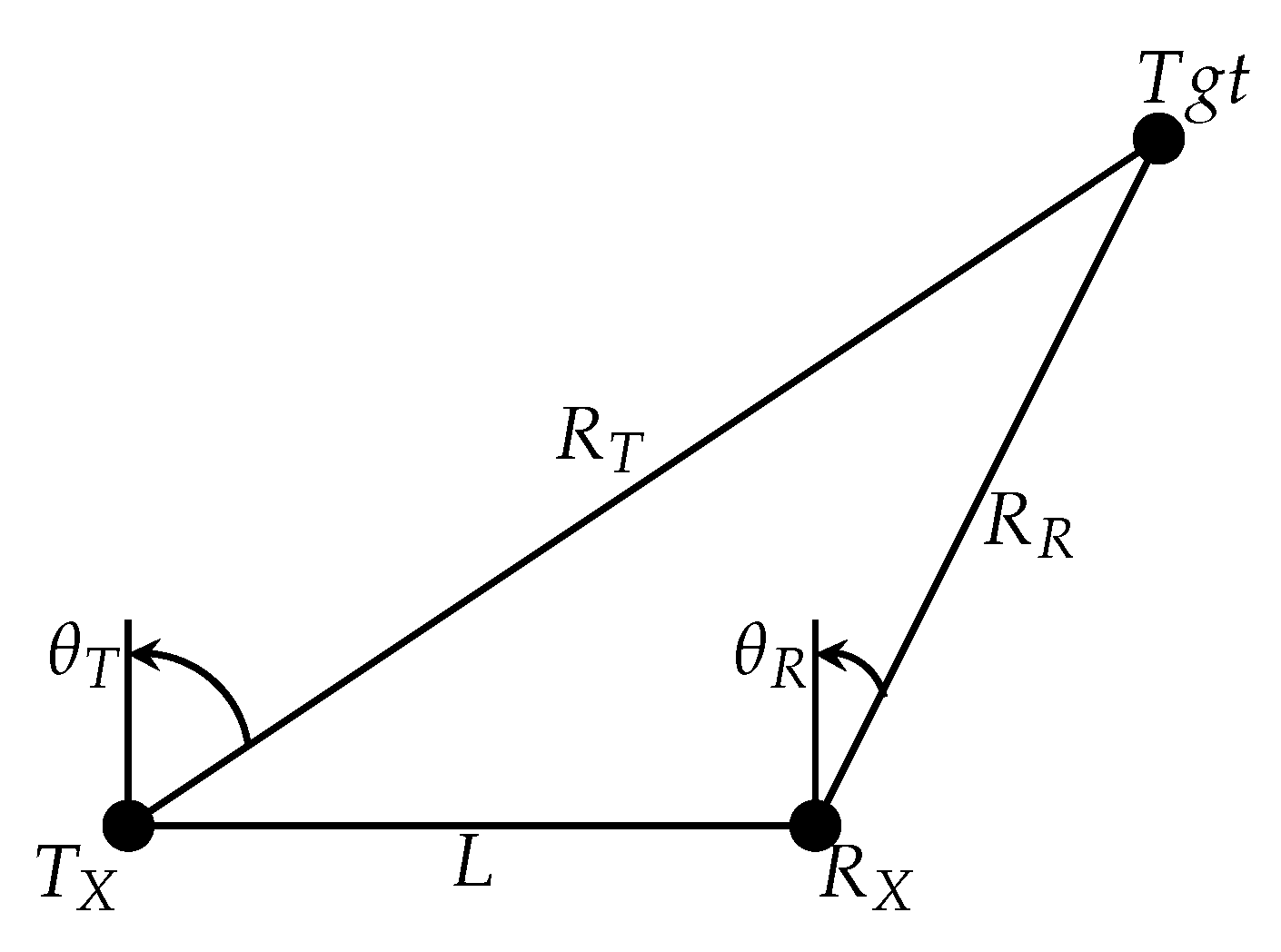
The bistatic radar shown in Figure 8 has the transmitter and receiver at different locations separated by a considerable distance called baseline (L). Compared to a monostatic radar, some advantages of using bistatic configuration are passive sensing, detection of low radar cross-sectional (RCS) targets, and avoiding jammer systems, etc. Despite these advantages, bistatic radars are not commonly employed due to their geometry and the problem associated with synchronization of the receiver and transmitter, which is necessary to obtain range-Doppler information of the target. In [55,56], tools such as global positioning systems (GPS), crystal oscillators, low-cost quartz GPS-disciplined oscillators, satellites, and wired communication channels, etc. are used to synchronize the receiver and the transmitter. Furthermore, due to the geometry limitations of bistatic radars, unique signal processing methods are required to obtain high-resolution imagery of targets. Instead, chaotic oscillators offer a cost-effective way of synchronizing bistatic radar receivers [57,58], as well as generating high-resolution radar imagery [59].

To synchronize and detect the target, we consider two antennas at the receiver. One is dedicated to face the transmitter, and the other is used to track the target. We assume that the transmitter and the receiver are in line-of-sight (LOS) and are on non-moving platforms. A direct synchronization approach is utilized at the bistatic radar receiver [60], as shown in Figure 9. Here, the synchronization is achieved directly by receiving a signal (through the dedicated antenna), demodulating it, and synchronizing the local oscillator to achieve the ranging and detection. Hence, the term direct synchronization. Usually, the signal transmission takes place using a separate channel such as a land-line cable, communication link, or a satellite. Instead, we propose using the transmitted CBFM waveform to achieve synchronization while providing excellent range resolution. The waveform incident on the dedicated antenna is demodulated using the PLL (with the same specifications) mentioned above. The scaled version of the output of PLL, i.e., $d\left(t\right)=\zeta p\left(t\right)$ is used to drive the local RCOs. Depending on the bit encoded at the transmitter, the RCO that is tuned with respective control parameters will be synchronized. That is, when a bit (−1) is encoded, the RCO₁ is synchronized, and when a bit (+1) is encoded, the RCO₂ is synchronized.

The comparator (given in Equation (6) or part of Figure 5) is used to determine which RCO is synchronized with the least error level. The normalized version of the corresponding RCO’s $\widehat{x}\left(t\right)$, i.e., ${\widehat{v}}_i\left(t\right)=\widehat{x}\left(t\right)/{\zeta }_r$ forms the instantaneous frequency to reconstruct the CBFM waveform. Here, ${\zeta }_r$ is maximum of $|\widehat{x}\left(t\right)|$. The reconstructed CBFM waveform $s_{rec}\left(t\right)$ given in Equation (8) serves as a reference waveform for the matched filter.

$$s_{rec}\left(t\right)=Aexp\left(j2\pi f_{c}t+j2\pi K\underset{0}{\overset{t}{\int }}{\widehat{v}}_i\left(\alpha \right)d\alpha \right).$$

(8)

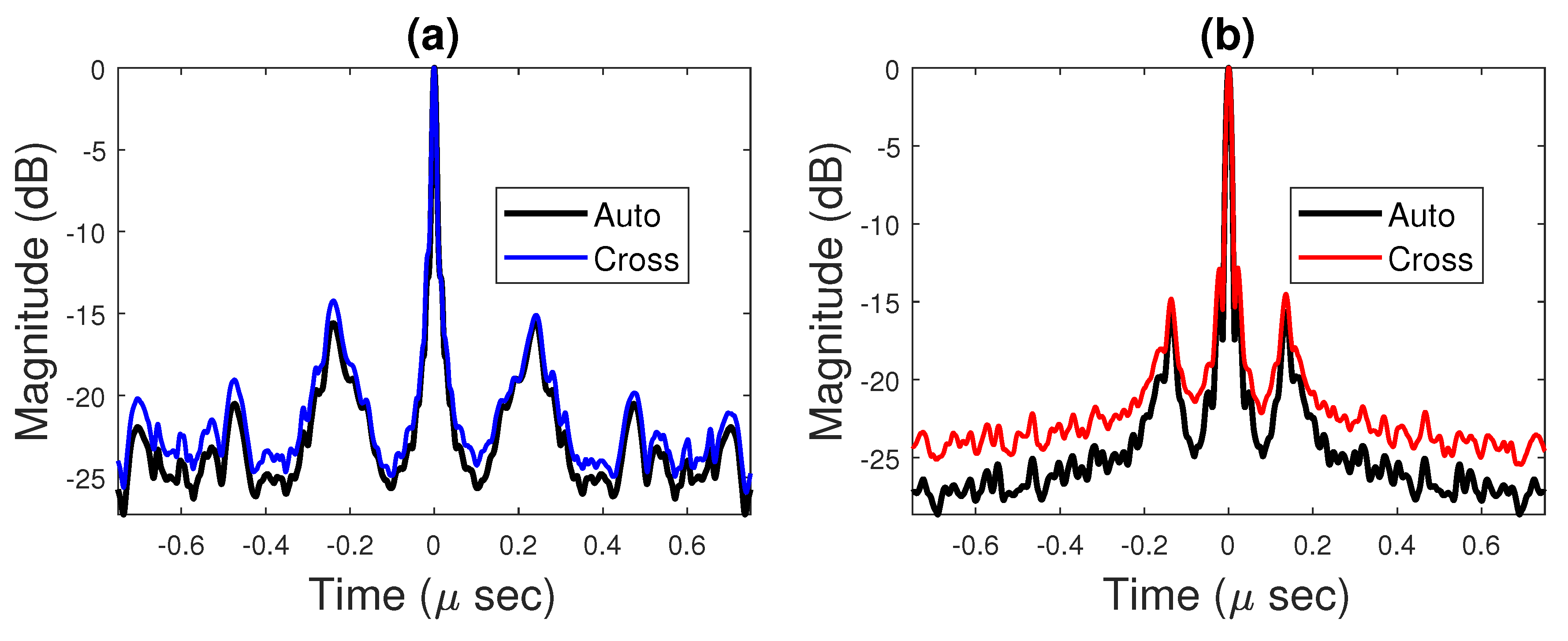
The effectiveness of the reconstruction approach is characterized using correlation analysis. In Figure 10a, the auto-correlation between $\left\{s\right(t),s(t\left)\right\}$ of the Lorenz CBFM is plotted using a solid line (black color) plot while the cross-correlation between $\{s\left(t\right),s_{rec}\left(t\right)\}$ is plotted in the blue color plot. Similarly, Figure 10b shows the auto-correlation in a solid line (black color) and cross-correlation (red color) plot for the Burke–Shaw CBFM waveform. In both instances, the cross-correlation closely replicates the auto-correlation of $s\left(t\right)$ with adjacent sidelobe levels (SLL) at $-13.33$ dB or below. These correlation properties show that the proposed synchronization method is effective for the bistatic radar system.

5.2. Cross-Ambiguity Functions

Once the bistatic radar receiver is synchronized and the transmitted waveform is reconstructed, $s_{rec}\left(t\right)$ is used to correlate with the echo from the target $r_{tgt}\left(t\right)$. This echo is a time-delayed and Doppler-shifted version of the transmitted waveform. That is

$$r_{tgt}\left(t\right)=s(t-\tau )ex{p}^{j2\pi [f_c+f_D]t}.$$

(9)

From Figure 8, let the range between the transmitter and the target be $R_T$, the range between the target and the receiver be $R_R$. The bistatic configuration where $L<R_R$ is called the cosite region, otherwise it is called the receiver-centered region. If ${\theta }_R$ is the receiver look angle, then the relationships between the time-delay $\tau$, range between the target-receiver $R_R$ and Doppler frequency $f_D$, and radial velocity V of the target are, respectively, given as [61]

$$\left(\tau =\frac{R_R+\sqrt{R_R^2+L^2+2R_{R}Lsin{\theta }_R}}{c};f_D=\frac{2f_c}{c}V\sqrt{\frac{1}{2}+\frac{R_R+Lsin{\theta }_R}{2\sqrt{R_R^2+L^2+2R_{R}Lsin{\theta }_R}}}\right)$$

(10)

where c is the speed of light. To detect a target, the bistatic radar parameters to be investigated are the estimates of time delay $\widehat{\tau }$ and the Doppler frequency ${\widehat{f}}_D$. Similar to Equation (10), they are expressed as

$$\left(\widehat{\tau }=\frac{{\widehat{R}}_R+\sqrt{{\widehat{R}}_R^2+L^2+2{\widehat{R}}_{R}Lsin{\theta }_R}}{c};{\widehat{f}}_D=\frac{2f_c}{c}\widehat{V}\sqrt{\frac{1}{2}+\frac{{\widehat{R}}_R+Lsin{\theta }_R}{2\sqrt{{\widehat{R}}_R^2+L^2+2{\widehat{R}}_{R}Lsin{\theta }_R}}}\right)$$

(11)

When the target echo is processed through the matched filter [62], the estimates $\widehat{\tau }$ and ${\widehat{f}}_D$ can be determined via the cross-ambiguity function $\chi \left(\widehat{\tau }-\tau ,{\widehat{f}}_D-f_D\right)$, which is expressed as Equation (12). However, due to the nonlinear relationship between $\{\widehat{\tau },{\widehat{R}}_R\}$ and $\{{\widehat{f}}_D,\widehat{V}\}$, the cross-ambiguity function of a bistatic radar is plotted on the range-velocity plane.

$$\chi \left(\widehat{\tau }-\tau ,{\widehat{f}}_D-f_D\right)=\underset{-\infty }{\overset{\infty }{\int }}s(t-\tau )s_{rec}^{*}(t-\widehat{\tau })ex{p}^{[-j2\pi \left(f_D-{\widehat{f}}_D\right)t]}dt.$$

(12)

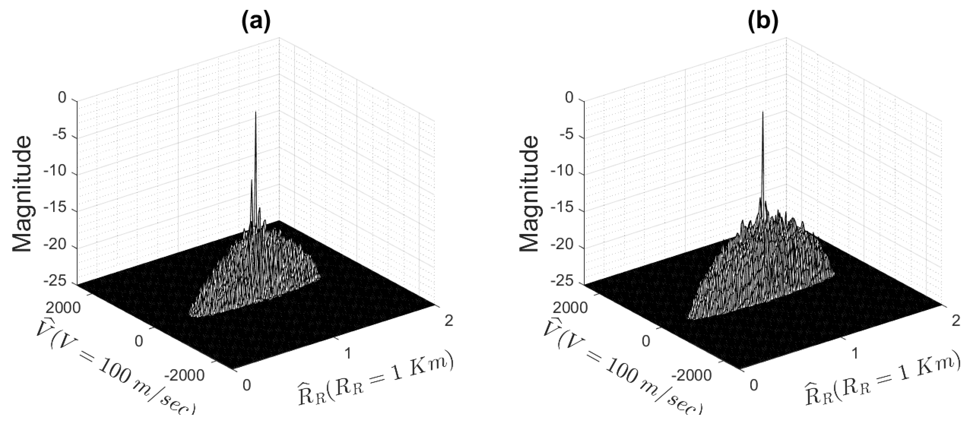
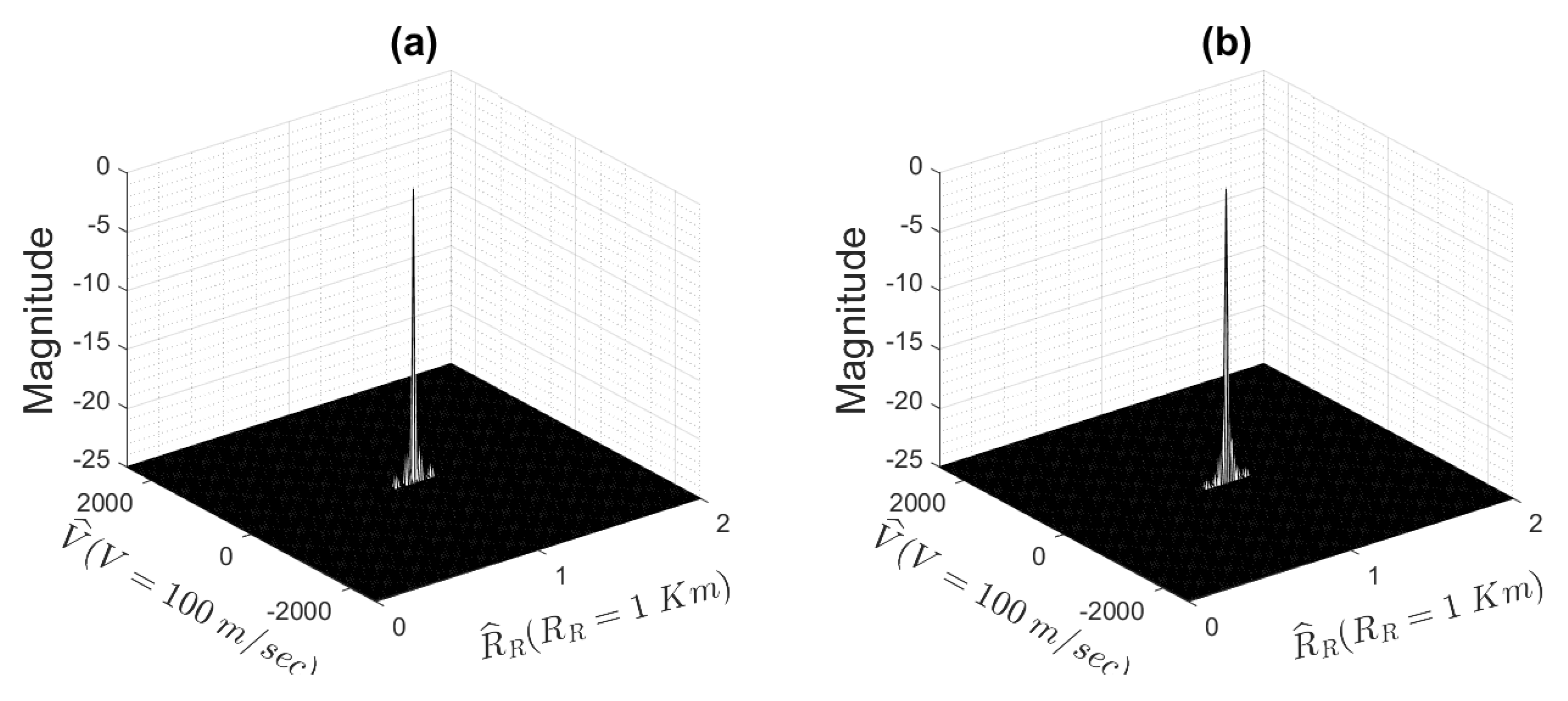
For the simulations, we considered a point target moving with a velocity $V_{tgt}=100$ m/s, $L=0.5$ Km, $R_R=1$ Km, and ${\theta }_R=+{30}^{\circ }$. When the received echo is driven through the matched filter with a response $s_{rec}\left(t\right)$, a peak is expected at $R_R$ and $V_{tgt}$. Figure 11a,b shows the cross-ambiguity surface of the Lorenz CBFM and the Burke–Shaw CBFM waveforms, respectively, which is computed between the $\{s_{rec}\left(t\right),r_{tgt}\left(t\right)\}$.

For the Lorenz CBFM waveform, the sidelobes on the velocity plane decorrelate very quickly. On the range plane, the first SLL occurs at $0.136(-17.3$ dB). The subsequent sidelobes disappear at a faster rate. Similarly, for the Burke–Shaw CBFM waveform, the first range SLL occurs at $0.081(-21.93$ dB). If the digital information is embedded onto the chirp signal, the corresponding ambiguity surface resembles a shape of the mountain ridge with range-Doppler coupling [14,15]. In contrast, the cross-ambiguity surface of the CBFM waveform closely resembles a thumb-tack ambiguity function with a significant peak occurring at $R_R=1$ Km and $V=100$ m/s.

5.3. Signature Analysis for the Bistatic Radar Configuration

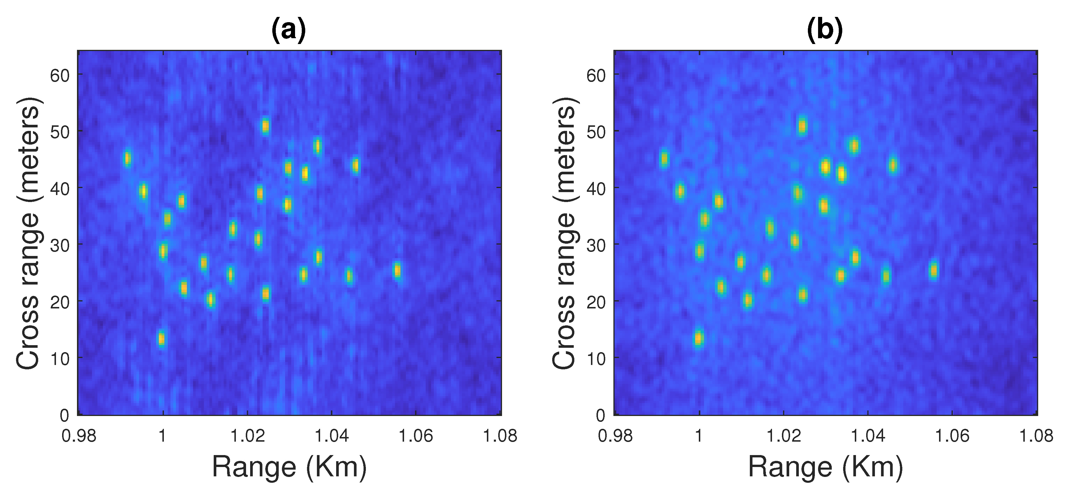
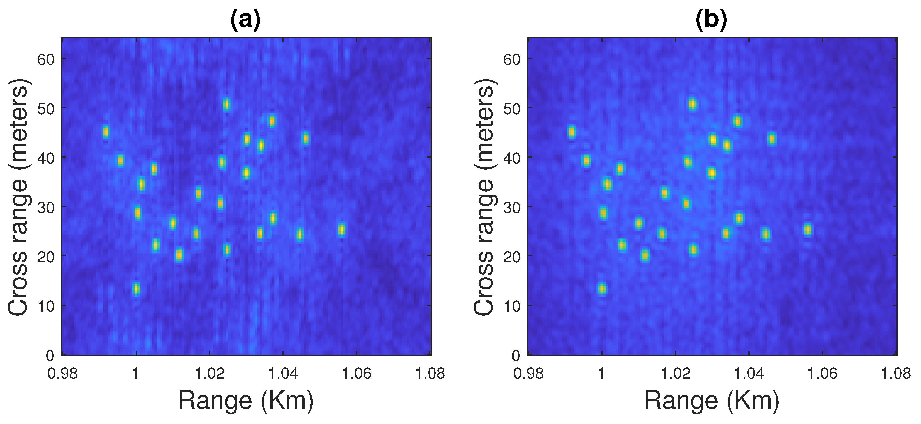
Due to the thumbtack cross-ambiguity surfaces, the CBFM waveforms make an excellent alternative for high-resolution radar imaging. A complex target such as an airplane consists of multiple point reflectors, also called hotspots [63]. Consequently, the received signal from a complex target is given as

$$r\left(t\right)=\sum _{k=1}^{N}s(t-{\tau }_k)ex{p}^{\left[j2\pi (f_c+f_{D_k})t\right]}.$$

(13)

When the received signal is applied to the matched filter with an impulse response $s_{rec}\left(t\right)$, multiple peaks associated with each hotspot’s range and velocity can be obtained, resulting in the signature of the complex target [64]. For example, Figure 12 shows the signature of the BOEING 777 airplane that consists of 24 point reflectors. All these hotspots are accurately resolved, illustrating the high-resolution capability of the proposed CBFM waveform as well as the synchronization approach. A complete study on generating a signature analysis of complex targets is shown in our previous work [59]. As mentioned, we assume the transmitters and receivers are on a non-moving platform. Moving platforms would require, at minimum, adaptive motion compensation to eliminate non-rotational Doppler shifts that would degrade range-Doppler imagery [65]. This analysis will be provided in our future work.

The quality of the radar image can be assessed using entropy-like functions [66]. The entropy of an image is given as

$$E=\frac{-{\displaystyle \sum _m}{\displaystyle \sum _n}{I}_{mn}lo{g}_2\left(I_{mn}\right)}{{\displaystyle \sum _m}{\displaystyle \sum _n}{I}_{mn}}.$$

(14)

In the above equation, m and n are the number of rows and columns of an image, and I is the normalized ambiguity surface such that the maximum pixel reflectivity is one. For an ideal thumbtack ambiguity function, the pixel value is either 0 or 1. Hence, the entropy value should be zero. Conversely, an increase in the entropy value indicates the presence of sidelobe and noise dominance.

Using Equation (14), the entropy of the signature generated using the Lorenz CBFM is 1.8605 and that of the Burke–Shaw CBFM waveform is 1.7860. The positive entropy values are apparent due to the increased noise-floor and self-noise of the transmitted waveform. As expected, the entropy values for both the CBFM waveforms are similar due to the same transmitted bandwidth. In either case, the high-resolution imagery of the signature is evident.

5.4. Cross-Ambiguity Functions in the Presence of Noise

To assess the proposed joint bistatic RadComm system, we further computed the cross-ambiguity functions in the presence of noise. The received signal from the transmitter is typically corrupted with noise that can be modeled as bandlimited additive white Gaussian noise (BL-AWGN) [62]. That is

$$r\left(t\right)=s\left(t\right)+\eta \left(t\right).$$

(15)

The same procedure as illustrated in Figure 9 is used to reconstruct the CBFM waveform at the bistatic radar receiver. Once the CBFM waveform is reconstructed in the presence of noise, it can be used to correlate with the target echo, which is also assumed to be corrupted with BL-AWGN. That is

$$r_{tgt}\left(t\right)=s(t-\tau )ex{p}^{j2\pi [f_c+f_D]t}+\eta \left(t\right).$$

(16)

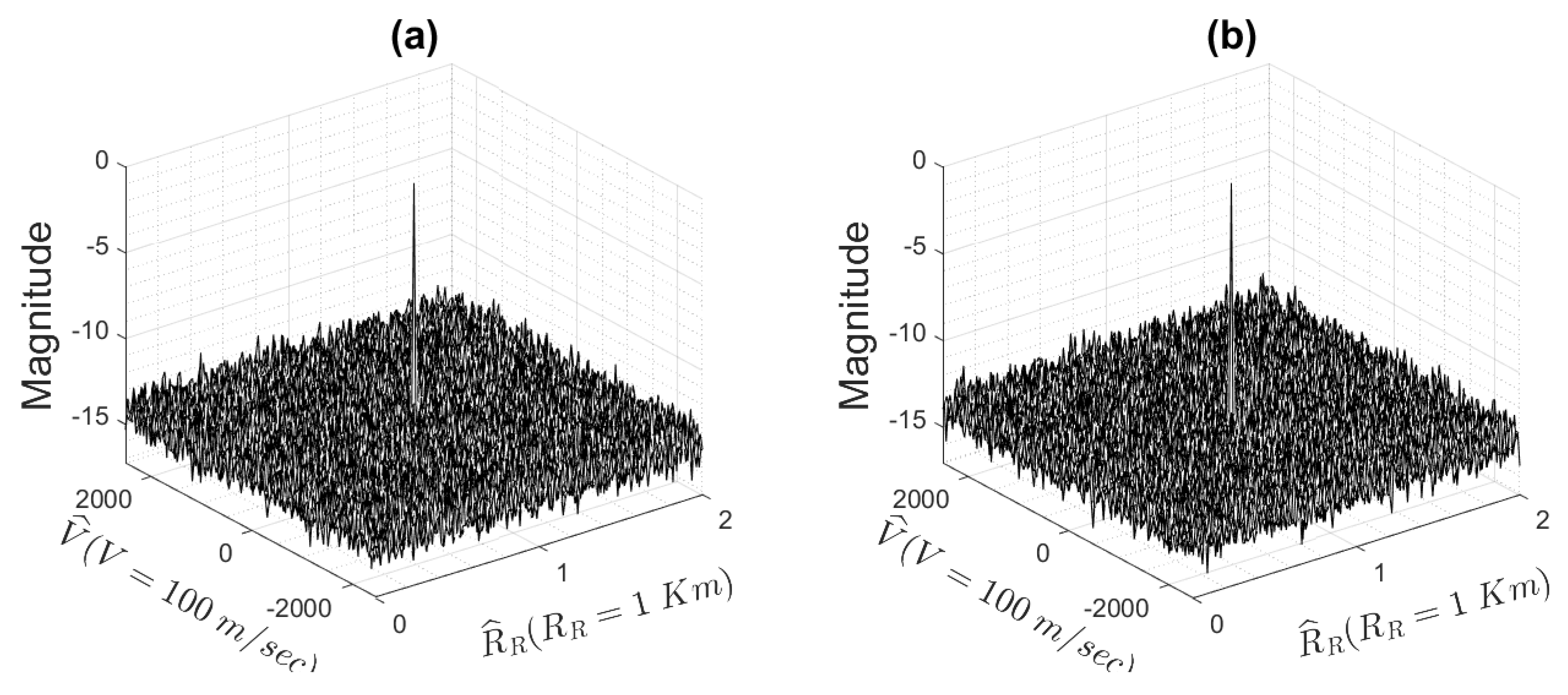
Figure 13a shows the cross-ambiguity functions between $\{r\left(t\right),r_{tgt}\}$ for the Lorenz CBFM waveform with an SNR of 3 dB. Figure 13b is for the Burke–Shaw CBFM waveform. In both cases, the noise floor tends to rise, and the energy from the mainlobe peak spills over to the adjacent sidelobes. While the sidelobes on the velocity plane were not affected, the range sidelobes for the Lorenz CBFM and the Burke–Shaw CBFM waveforms were raised to $-11.5$ and $-13.5$ dB, respectively. The sidelobes adjacent to the mainlobe could be further reduced using standard Chebyshev windows.

The bistatic radar synchronization using chaos and reconstruction of the FM waveform is susceptible to very high noise levels. It is because the self-synchronization of the chaotic system is sensitive to parameter mismatch and noise [53]. Furthermore, since the bistatic radar receiver employs the self-synchronization scheme, the reconstruction of the FM waveform suffers in the presence of noise, especially if SNR is less than 3 dB.

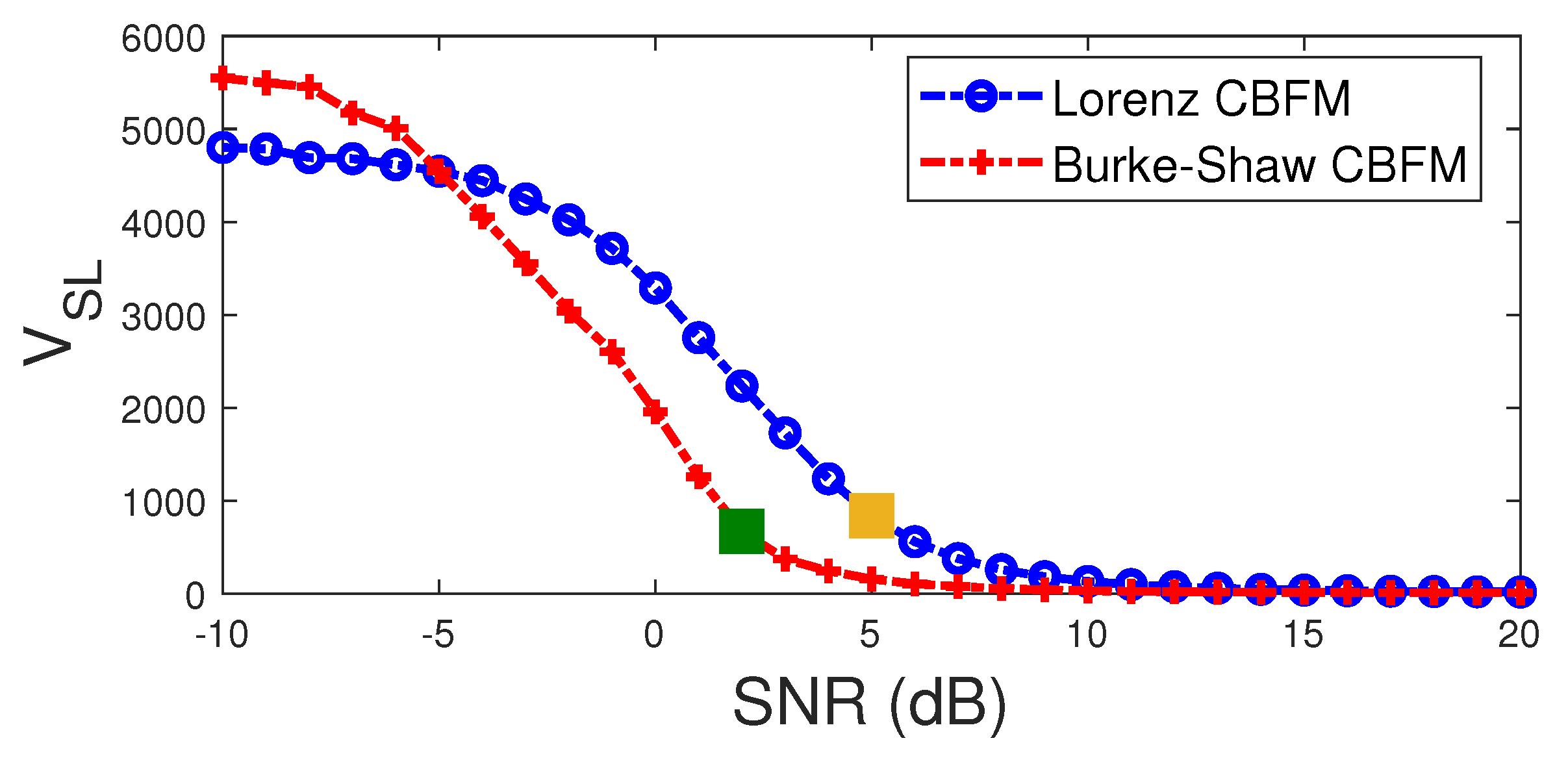
The quality of the simulated cross-ambiguity functions in the presence of noise can be evaluated using the sidelobe volume function [67] given in Equation (17). For an ideal thumbtack ambiguity function, $V_{SL}$ should be equal to zero. Any positive value indicates the presence of sidelobes and an increase in noise-floor. It may not provide information about the value of SLL, but it conveys the quality of the ambiguity function by computing the overall sidelobes adjacent to the prominent peak.

$$V_{SL}=\underset{f}{\int }\underset{t}{\int }{\left|\chi \right|}^{2}dtdf-\underset{-\Delta f}{\overset{\Delta f}{\int }}\underset{-\Delta t}{\overset{\Delta t}{\int }}{\left|\chi \right|}^{2}dtdf.$$

(17)

Figure 14 shows the sidelobe volume of the CBFM waveforms in bistatic configuration plotted against the SNR. As the noise increases, there is a clear indication of the growth of SLL. Overall the Burke–Shaw CBFM waveform outperforms the Lorenz CBFM waveform. For the Lorenz CBFM waveform, as indicated in the gold color square, the reference SLL of $-13.33$ dB occurs for $SNR=5$ dB, while for the Burke–Shaw CBFM waveform, it appears for $SNR=2$ dB (indicated in the green square). A detailed study on the bistatic radar synchronization using the CBFM waveform and its high-resolution capabilities is presented in [59].

The Burke–Shaw CBFM waveform has better performance in terms of sidelobe volume because of its apparent random behavior compared to the Lorenz CBFM waveform. It can be observed by looking at the time series plot, as shown in Figure 2, as well as the higher value of the largest Lyapunov exponent, indicating a more chaotic nature of the waveform.

6. Monostatic Radar Signal Processing

6.1. Ambiguity Surface of Monostatic CBFM Radar

For a monostatic radar configuration, the transmitter and receiver are collocated. Therefore, additional procedures as shown for the bistatic configuration are not necessary. The same waveform that is embedded with digital information $i\left(t\right)$ is used for efficient transmission. The response of the matched filter is $s\left(t\right)$. Hence, the ambiguity function in monostatic configuration is given as

$$\chi \left(\widehat{\tau }-\tau ,{\widehat{f}}_D-d_D\right)=\underset{-\infty }{\overset{\infty }{\int }}s(t-\tau )s^{*}(t-\widehat{\tau })ex{p}^{[-j2\pi \left(f_D-{\widehat{f}}_D\right)t]}dt.$$

(18)

In the above equation,

$$\left(\tau =\frac{2R_R}{c};f_D=\frac{2f_c}{c}V\right)$$

(19)

$$\left(\widehat{\tau }=\frac{2{\widehat{R}}_R}{c};{\widehat{f}}_D=\frac{2f_c}{c}\widehat{V}\right)$$

(20)

Since the relationship between the range-delay and velocity-Doppler frequency is linear, the ambiguity surface can be plotted either on the delay-Doppler plane, which is traditionally used or on the range-velocity plane. Figure 15 shows the ambiguity surface of the CBFM waveforms on the range-velocity plane. For both the Lorenz CBFM (Figure 15a) and the Burke–Shaw CBFM waveforms (Figure 15b), a near thumbtack ambiguity function is obtained. Similar to the bistatic radar, the sidelobes on the velocity plane die out very quickly. The sidelobes on the range plane for the Lorenz CBFM is at 0.055 ($-25.2$ dB), and for the Burke–Shaw CBFM, it is at 0.052 ($-25.7$ dB). These extremely low sidelobes prove that the CBFM waveforms serve as an excellent candidate for high-resolution radar imaging.

6.2. Signature Analysis for the Monostatic Radar Configuration

As mentioned earlier, in the presence of a complex target, the received is the summation of reflections from multiple point reflectors. Each of these reflections is delayed and Doppler-shifted depending on the location of the reflector. Hence, when the received signal is processed through the matched filter with impulse response $s\left(t\right)$, the resultant is the signature analysis. Note that for the bistatic radar, the matched filter response is $s_{rec}\left(t\right)$. Figure 16 shows the signature analysis of the same complex target. In addition, the entropy of the Lorenz and Burke–Shaw CBFM waveforms is close to 2. The positive entropy value signifies the presence of self-noise and a rise in the noise-floor of the signature. However, all the hotspots are distinguishable from each other.

6.3. Ambiguity Functions in the Presence of Noise

Since the monostatic radar configuration does not require a chaotic synchronization approach, its performance in the presence of noise is robust compared to the bistatic radar system. Consequently, even for the SNR of $-30$ dB, the sidelobe does not rise above $-13.33$ dB. Figure 17a,b shows the ambiguity surface of the Lorenz CBFM and Burke–Shaw CBFM waveforms considering the received signal is corrupted with $SNR=-30$ dB. The noise floor rises uniformly to 0.21 $(-13.5$ dB) across both planes. From Figure 18 it is evident that for $SNR<-30$ dB, the sidelobes increase significantly, likely masking the targets present in close proximity.

7. Conclusions

In this work, we presented a waveform design for joint monostatic radar-communication and bistatic radar-communication systems. The generation of such a waveform is possible using a chaotic oscillator modeled as nonlinear differential equations. The digital information is embedded onto the chaotic oscillator using chaos shift keying. The resultant output of the oscillator is used as an instantaneous frequency to generate a chaos-based frequency-modulated waveform. This CBFM waveform is used for the dual application of radar detection and communications.

We presented a nonlinear detection scheme to decode the digital information. Here, we used two synchronized chaotic oscillators to compare the error difference to determine the encoded bit. Through simulations, we showed that the bit error rate of the CBFM waveform closely matches the bipolar shift keying.

The same nonlinear detection scheme is used at the bistatic radar receiver to synchronize it with the transmitter. We use the synchronized local response oscillator to reconstruct the transmitted FM waveform, which acts as the response for the matched filter. The cross-ambiguity functions revealed a sharp mainlobe peak with minimum sidelobes on the range-velocity planes desirable for high-resolution radar imaging. Signature analysis of the complex target revealed the high-resolution capability of the proposed waveform. However, due to the noise sensitivity of the nonlinear detector, our proposed approach is susceptible to a significant amount of noise levels.

The self-ambiguity surface of CBFM waveforms for monostatic radars is of high quality. The sidelobes on the range-velocity planes are extremely low. The signature analysis illustrates that all the point reflectors could be distinguished accurately. In contrast to the bistatic configuration, the monostatic radar performed excellently for SNRs as low as $-30$ dB.

Our proposed work can have potential in airplanes, emergency response vehicles, and defense sectors where faster communication rates and accurate target detection are necessary. With the proposed work, both of these are achievable in addition to secure communications and high-resolution imagery.

References

- Tavik, G.C.; Hilterbrick, C.L.; Evins, J.B.; Alter, J.J.; Crnkovich, J.G.; de Graaf, J.W.; Habicht, W., II; Hrin, G.P.; Lessin, S.A.; Wu, D.C.; et al. The advanced multifunction RF concept. IEEE Trans. Microw. Theory Tech. 2005, 53, 1009–1020. [Google Scholar] [CrossRef]
- Griffiths, H.; Cohen, L.; Watts, S.; Mokole, E.; Baker, C.; Wicks, M.; Blunt, S. Radar spectrum engineering and management: Technical and regulatory issue. Proc. IEEE 2015, 103, 85–102. [Google Scholar] [CrossRef]
- Zheng, L.; Lops, M.; Eldar, Y.C.; Wang, X. Radar and Communication Coexistence: An Overview: A Review of Recent Methods. IEEE Signal Process. Mag. 2019, 36, 85–99. [Google Scholar] [CrossRef]
- Cohen, D.; Mishra, K.V.; Eldar, Y.C. Spectrum sharing radar: Coexistence via Xampling. IEEE Trans. Aerosp. Electron. Syst. 2017, 54, 1279–1296. [Google Scholar] [CrossRef]
- Li, B.; Petropulu, A.P.; Trappe, W. Optimum co-design for spectrum sharing between matrix completion based MIMO radars and a MIMO communication system. IEEE Trans. Signal Process. 2016, 64, 4562–4575. [Google Scholar] [CrossRef] [Green Version]
- Qian, J.; Lops, M.; Zheng, L.; Wang, X.; He, Z. Joint system design for coexistence of MIMO radar and MIMO communication. IEEE Trans. Signal Process. 2018, 66, 3504–3519. [Google Scholar] [CrossRef]
- Li, B.; Petropulu, A.P. Joint transmit designs for coexistence of MIMO wireless communications and sparse sensing radars in clutter. IEEE Trans. Aerosp. Electron. Syst. 2017, 53, 2846–2864. [Google Scholar] [CrossRef]
- Liu, F.; Christos, M.; Petropulu, A.; Griffiths, H.; Hanzo, L. Joint radar and communication design: Applications, state-of-the-art, and the road ahead. IEEE Trans. Commun. 2020, 68, 3834–3862. [Google Scholar] [CrossRef] [Green Version]
- Deng, H.; Himed, B. Interference Mitigation Processing for Spectrum-Sharing Between Radar and Wireless Communications Systems. IEEE Trans. Aerosp. Electron. Syst. 2013, 49, 1911–1919. [Google Scholar] [CrossRef]
- Kumar, S.; Mishra, K.V.; Gautam, S.; Mysore, B.S.; Ottersten, B. Interference Mitigation Methods for Coexistence of Radar and Communication. In Proceedings of the 15th European Conference on Antennas and Propagation (EuCAP), Dusseldorf, Germany, 22–26 March 2021; pp. 1–4. [Google Scholar]
- Han, L.; Wu, K. Joint wireless communication and radar sensing systems-state of the art and future prospects. IET Microwaves, Antennas Propag. 2013, 7, 876–885. [Google Scholar] [CrossRef]
- Blunt, S.D.; Yatham, P.; Stiles, J. Intrapulse Radar-Embedded Communications. IEEE Trans. Aerosp. Electron. Syst. 2010, 46, 1185–1200. [Google Scholar] [CrossRef]
- Huang, K.W.; Bica, M.; Mitra, U.; Koivunen, V. Radar waveform design in spectrum sharing environment: Coexistence and cognition. In Proceedings of the IEEE Radar Conference (RadarCon), Arlington, VA, USA, 10–15 May 2015; pp. 1698–1703. [Google Scholar]
- Zhang, Z.; Nowak, M.J.; Wicks, M.C.; Wu, Z. Bio-inspired RF steganography via linear chirp radar signals. IEEE Commun. Mag. 2016, 54, 82–86. [Google Scholar] [CrossRef]
- Zhang, Z.; Qu, Y.; Wu, Z.; Nowak, M.J.; Ellinger, J.; Wicks, M.C. RF steganography via LFM chirp radar signals. IEEE Trans. Aerosp. Electron. Syst. 2017, 54, 1221–1236. [Google Scholar] [CrossRef]
- Hassanien, A.; Amin, M.G.; Zhang, Y.D.; Ahmad, F. Phase-modulation based dual-function radar-communications. IET Radar Sonar Navig. 2016, 10, 1411–1421. [Google Scholar] [CrossRef] [Green Version]
- Washington, R.; Bischof, B.; Garmatyuk, D.; Mudaliar, S. Clutter-Masked Waveform Design for LPI/LPD Radarcom Signal Encoding. Sensors 2021, 21, 631. [Google Scholar] [CrossRef]
- Bekar, M.; Baker, C.J.; Hoare, H.G.; Gashinova, M. Joint MIMO Radar and Communication System Using a PSK-LFM Waveform With TDM and CDM Approaches. IEEE Sens. J. 2021, 21, 6115–6124. [Google Scholar] [CrossRef]
- Hassanien, A.; Amin, M.G.; Aboutanios, E.; Himed, B. Dual-Function Radar Communication Systems: A Solution to the Spectrum Congestion Problem. IEEE Signal Process. Mag. 2019, 36, 115–126. [Google Scholar] [CrossRef]
- Wehner, D.R. High-Range Resolution Waveforms and Processing. In High-Resolution Radar, 2nd ed.; Artech House: Boston, MA, USA, 1994; pp. 133–194. [Google Scholar]
- Lathi, B.P.; Ding, Z. Performance analysis of digital communication systems. In Modern Digital and Analog Communication Systems, 4th ed.; Oxford University Press: New York, NY, USA, 2009; pp. 506–581. [Google Scholar]
- Surender, S.C.; Narayanan, R.M. UWB noise-OFDM netted radar: Physical layer design and analysis. IEEE Trans. Aerosp. Electron. Syst. 2011, 47, 1380–1400. [Google Scholar] [CrossRef]
- Kocarev, L.; Halle, K.S.; Eckert, K.; Chua, L.O.; Parlitz, U. Experimental Demonstration of Secure Communications via Chaotic Synchronization. Int. J. Bifurcations Chaos Appl. Sci. Technol. 1992, 2, 709–713. [Google Scholar] [CrossRef]
- Cuomo, K.M.; Oppenheim, A.V. Circuit Implementation of Synchronized Chaos with Applications to Communications. Phys. Rev. Lett. 1993, 71, 65–68. [Google Scholar] [CrossRef]
- Dedieu, H.; Kennedy, M.P.; Hasler, M. Chaos shift keying: Modulation and demodulation of a chaotic carrier using self-synchronizing Chua’s circuits. IEEE Trans. Circuits Syst. II Analog. Digit. Signal Process. 1993, 40, 634–642. [Google Scholar] [CrossRef]
- Kolumban, G.; Kennedy, M.P.; Chua, L.O. The Role of Synchronization in Digital Communications Using Chaos-Part I: Fundamentals of Digital Communications. IEEE Trans. Circuits Syst.-Part I Fundam. Theory Appl. 1997, 44, 927–935. [Google Scholar] [CrossRef] [Green Version]
- Mazzini, G.; Setti, G.; Rovatti, R. Chaotic complex spreading sequences for asynchronous DS-CDMA. I. System modeling and results. IEEE Trans. Circuits-Syst.-Part I Fundam. Theory Appl. 1997, 44, 937–947. [Google Scholar] [CrossRef]
- Rulkov, N.F.; Tsimring, L. Communication with Chaos over Band-Limited Channels. Int. J. Circuit Theory Appl. 1999, 27, 555–567. [Google Scholar] [CrossRef]
- Abel, A.; Schwartz, W.; Goetz, M. Noise Performance of Chaotic Communication Systems. IEEE Trans. Circuits-Syst.-Part I Fundam. Theory Appl. 2000, 47, 1726–1732. [Google Scholar] [CrossRef]
- Williams, C. Chaotic Communications over Radio Channels. IEEE Trans. Circuits Syst.-Part I Fundam. Theory Appl. 2001, 48, 1394–1404. [Google Scholar] [CrossRef]
- Abel, A.; Schwarz, W. Chaos communications-principles, schemes, and system analysis. Proc. IEEE 2002, 90, 691–710. [Google Scholar] [CrossRef]
- Argyris, A.; Syvridis, D.; Larger, L.; Annovazzi-Lodi, V.; Colet, P.; Fischer, I.; Garcia-Ojalvo, J.; Mirasso, C.R.; Pesquera, L.; Shore, K.A. Chaos-based communications at high bit rates using commercial fibre-optic links. Nature 2005, 438, 343–346. [Google Scholar] [CrossRef] [PubMed]
- Blakely, J.N.; Hahs, D.W.; Corron, N.J. Communication waveform properties of an exact folded-band chaotic oscillator. Phys. D Nonlinear Phenom. 2013, 263, 99–106. [Google Scholar] [CrossRef]
- Kaddoum, G.; Soujeri, E. NR-DCSK: A Noise Reduction Differential Chaos Shift Keying System. IEEE Trans. Circuits Syst. II Express Briefs 2016, 63, 648–652. [Google Scholar] [CrossRef] [Green Version]
- Myneni, K.; Barr, T.A.; Reed, B.R.; Pethel, S.D.; Corron, N.J. High-precision ranging using a chaotic laser pulse train. Appl. Phys. Lett. 2001, 78, 1496–1498. [Google Scholar] [CrossRef]
- Beal, A.N.; Cohen, S.D.; Syed, T.M. Generating and detecting solvable chaos at radio frequencies with consideration to multi-user ranging. Sensors 2020, 20, 774. [Google Scholar] [CrossRef] [PubMed] [Green Version]
- Flores, B.C.; Solis, E.A.; Thomas, G. Assessment of chaos-based FM signals for range–Doppler imaging. IEE Proc.-Radar Sonar Navig. 2003, 150, 313–322. [Google Scholar] [CrossRef]
- Lin, F.; Liu, J. Ambiguity functions of laser-based chaotic radar. IEEE J. Quantum Electron. 2004, 40, 1732–1738. [Google Scholar] [CrossRef]
- Liu, Z.; Zhu, X.; Hu, W.; Jiang, F. Principles of chaotic signal radar. Int. J. Bifurc. Chaos 2007, 17, 1735–1739. [Google Scholar] [CrossRef]
- Shi, Z.; Qiao, S.; Chen, K.S.; Cui, W.; Ma, W.; Jiang, T.; Ran, L. Ambiguity functions of direct chaotic radar employing microwave chaotic Colpitts oscillator. Prog. Electromagn. Res. 2007, 77, 1–14. [Google Scholar] [CrossRef] [Green Version]
- Willsey, M.S.; Cuomo, K.M.; Oppenheim, A.V. Quasi-orthogonal wideband radar waveforms based on chaotic systems. IEEE Trans. Aerosp. Electron. Syst. 2011, 47, 1974–1984. [Google Scholar] [CrossRef] [Green Version]
- Sprott, J.C. Introduction. In Chaos and Time-Series Analysis; Oxford University Press: New York, NY, USA, 2003; pp. 1–19. [Google Scholar]
- Sprott, J.C. Strange Attractors. In Chaos and Time-Series Analysis; Oxford University Press: New York, NY, USA, 2003; pp. 127–158. [Google Scholar]
- Lorenz, E.N. Synchronisation of bistatic radar systems. J. Atmos. Sci. 1963, 20, 130–141. [Google Scholar] [CrossRef] [Green Version]
- Shaw, R. Strange attractors, chaotic behavior, and information flow. Z. Für Naturforschung 1981, 36, 80–112. [Google Scholar] [CrossRef]
- Chua, L.O.; Wu, C.W.; Huang, A.; Zhong, G.Q. A universal circuit for studying and generating chaos—Part. I: Routes to chaos. IEEE Trans. Circuits Syst. I Fundam. Theory Appl. 1993, 40, 732–744. [Google Scholar] [CrossRef]
- Carroll, T.L. Chaotic communications that are difficult to detect. Phys. Rev. E 2003, 67, 026207-1–026207-6. [Google Scholar] [CrossRef]
- Tlelo-Cuautle, E.; Mu noz-Pacheco, J.M.; Martínez-Carballido, J. Frequency scaling simulation of Chua’s circuit by automatic determination and control of step-size. Appl. Math. Comput. 2007, 194, 486–491. [Google Scholar] [CrossRef]
- Cuenot, J.B.; Larger, L.; Goedgebuer, J.P.; Rhodes, W.T. Chaos shift keying with an optoelectronic encryption system using chaos in wavelength. IEEE J. Quantum Electron. 2001, 37, 849–855. [Google Scholar] [CrossRef]
- Geist, K.; Parlitz, U.; Lauterborn, W. Comparison of different methods for computing Lyapunov exponents. Prog. Theor. Phys. 1990, 83, 875–893. [Google Scholar] [CrossRef]
- Li, C.; Sprott, J.C. Amplitude control approach for chaotic signals. Nonlinear Dyn. 2013, 73, 1335–1341. [Google Scholar] [CrossRef] [Green Version]
- Pecora, L.M.; Carroll, T.L. Synchronization in Chaotic Systems. Phys. Rev. Lett. 1990, 64, 821–824. [Google Scholar] [CrossRef]
- Pecora, L.M.; Carroll, T.L. Synchronization of chaotic systems. Chaos Interdiscip. J. Nonlinear Sci. 2015, 25, 097611. [Google Scholar] [CrossRef] [PubMed]
- Ziemer, R.E.; Tranter, W.H. Angle Modulation and Multiplexing. In Principles of Communication Systems, Modulation and Noise, 7th ed.; John Wiley & Sons: Hoboken, NJ, USA, 2014; pp. 156–213. [Google Scholar]
- Weib, M. Synchronisation of bistatic radar systems. IEEE Int. Geosci. Remote Sens. Symp. (IGARSS) 2004, 3, 1750–1753. [Google Scholar]
- Sandenbergh, J.S. Synchronising Coherent Networked Radar using Low-Cost GPS-Disciplined Oscillators. Ph.D. Thesis, University of Cape Town, Cape Town, South Africa, 2019. [Google Scholar]
- Carroll, T.L. Chaotic system for self-synchronizing Doppler measurement. Chaos Interdiscip. J. Nonlinear Sci. 2005, 15, 013109-1–013109-5. [Google Scholar] [CrossRef] [PubMed]
- Sorrentino, F.; DeLellis, P. Estimation of communication-delays through adaptive synchronization of chaos. Chaos Solitons Fractals 2012, 45, 35–46. [Google Scholar] [CrossRef] [Green Version]
- Pappu, C.S.; Flores, B.C. High Resolution Imaging of Chaotic Bistatic Radar. IEEE Trans. Aerosp. Electron. Syst. 2011, 56, 871–886. [Google Scholar] [CrossRef]
- Willis, N.J. Special Problems and Requirements. In Bistatic Radar; Scitech Publishing Inc.: Raleigh, NC, USA, 2005; pp. 245–260. [Google Scholar]
- Tsao, T.; Slamani, M.; Varshney, P.; Weiner, D.; Schwarzlander, H.; Borek, S. Ambiguity function for a bistatic radar. IEEE Trans. Aerosp. Electron. Syst. 1997, 33, 1041–1051. [Google Scholar] [CrossRef]
- Trees, H.L. Parameter estimation: Slowly-Fluctuating point targets. In Detection, Estimation, and Modulation Theory, Part III: Radar-Sonar Signal Processing and Gaussian Signals in Noise; Wiley: New York, NY, USA, 2001; pp. 275–340. [Google Scholar]
- Borkar, V.G.; Ghosh, A.; Singh, R.K.; Chourasia, N.K. Radar cross-section measurement techniques. Def. Sci. J. 2010, 60, 204. [Google Scholar] [CrossRef]
- Chen, V.C.; Qian, S. Joint time-frequency transform for radar range-Doppler imaging. IEEE Trans. Aerosp. Electron. Syst. 1998, 34, 486–499. [Google Scholar] [CrossRef]
- Son, J.S.; Thomas, G.; Flores, B.C. ISAR Concepts. In Range-Doppler Radar Imaging and Motion Compensation; Artech House: Boston, MA, USA, 2001; pp. 9–25. [Google Scholar]
- Flores, B.C.; Ugarte, A.; Kreinovich, V. Choice of an entropy-like function for range-Doppler processing. Autom. Object Recognit. III Int. Soc. Opt. Photonics (SPIE) 1993, 1960, 47–56. [Google Scholar]
- Abramovich, Y.I.; Frazer, G.J. Bounds on the volume and height distributions for the mimo radar ambiguity function. IEEE Signal Process. Lett. 2008, 15, 505–508. [Google Scholar] [CrossRef]
Figure 1.
Bifurcation plot of (a) the Lorenz system with varying parameter and (b) the Burke–Shaw system with varying parameter V.
Figure 2.
Instantaneous frequency ( is the scaled version of ) of the CBFM waveform using (a) Lorenz and (b) Burke–Shaw chaotic systems (zoom in plots). The solid line indicates the encoded information. The time-series plot does not have any discontinuities when digital information is encoded.
Figure 3.
Illustration of the joint radar-communication systems.
Figure 4.
Block diagram for the joint mono and bistatic RadComm transmitter.
Figure 5.
Proposed architecture for the communication receiver.
Figure 6.
Encoded information and errors and for (a) the Lorenz CBFM waveform and (b) Burke–Shaw CBFM waveform. (Illustration purpose only. For practical reasons, a single CBFM pulse transmits only one bit of information.)
Figure 7.
Bit error rate () for BPSK, Lorenz CBFM and Burke–Shaw CBFM waveforms, and BRPSK as a function of the ratio of energy per bit to noise spectral density ().
Figure 8.
Bistatic radar configuration.
Figure 9.
Architecture for the bistatic radar receiver.
Figure 10.
Auto–correlation (solid line plot) between and cross–correlation between for (a) the Lorenz CBFM waveform (blue color plot) and (b) the Burke–Shaw CBFM waveform (red color plot).
Figure 11.
Cross–ambiguity surface between for (a) the Lorenz CBFM waveform and (b) the Burke–Shaw CBFM waveform.
Figure 12.
Signature analysis of the complex target obtained using (a) the Lorenz CBFM waveform and (b) the Burke–Shaw CBFM waveform.
Figure 13.
The cross–ambiguity surface obtained using (a) the Lorenz CBFM waveform and (b) the Burke–Shaw CBFM waveform considering the dB.
Figure 14.
Sidelobe volume of the bistatic radar configuration for the Lorenz CBFM and Burke–Shaw CBFM waveforms plotted against the signal to noise ratio (). The squares indicate that for the respective SNR, the sidelobe levels are at the value of dB.
Figure 15.
Ambiguity surface of Monostatic radar for (a) the Lorenz CBFM waveform and (b) the Burke–Shaw CBFM waveform.
Figure 16.
Ambiguity surface of the monostatic radar for (a) the Lorenz CBFM waveform and (b) the Burke–Shaw CBFM waveform.
Figure 17.
Ambiguity surface of the monostatic radar for (a) the Lorenz CBFM waveform and (b) the Burke–Shaw CBFM waveform considering dB.
Figure 18.
Sidelobe volume of the monostatic radar configuration for the Lorenz CBFM and Burke–Shaw CBFM waveforms plotted against the signal to noise ratio (). The green square at dB indicate that for sidelobe levels are at the value of dB.