
Time-Varying Vibration Compensation Based on Segmented Interference for Triangular FMCW LiDAR Signals
by
 , and
, and
Rongrong Wang
1,2, 
Bingnan Wang
1,*,
Yachao Wang
1,
Wei Li
1,2,
Zhongbin Wang
1,2 and
Maosheng Xiang
1,2 1
National Key Laboratory of Microwave Imaging Technology, Aerospace Information Research Institute, Chinese Academy of Sciences, Beijing 100190, China
2
School of Electronics, Electrical and Communication Engineering, University of Chinese Academy of Sciences, Beijing 100049, China
*
Author to whom correspondence should be addressed.
Remote Sens. 2021, 13(19), 3803; https://doi.org/10.3390/rs13193803
Submission received: 24 June 2021
/
Revised: 16 September 2021
/
Accepted: 20 September 2021
/
Published: 23 September 2021
Abstract
:Frequency modulation continuous wave (FMCW) light detection and ranging (LiDAR) 3D imaging system may suffer from time-varying vibrations which will affect the accuracy of ranging and imaging of a target. The system uses only a single-period FMCW LiDAR signal to measure the range of each spot; however, traditional methods may not work well to compensate for the time-varying vibrations in a single period because they generally assume the vibration velocity is constant. To solve this problem, we propose a time-varying vibration compensation method based on segmented interference. We first derive the impact of time-varying vibrations on the range measurement of the FMCW LiDAR system, in which we divide the time-varying vibration errors into primary errors caused by the vibrations with a constant velocity and quadratic errors. Second, we estimate the coefficients of quadratic vibration errors by using a segmented interference method and build a quadratic compensation filter to eliminate the quadratic vibration errors from the original signals. Finally, we use the symmetrical relations of signals in a triangular FMCW period to estimate the vibration velocity and establish a primary compensation filter to eliminate the primary vibration errors. Numerical tests verify the applicability of this method in eliminating time-varying vibration errors with only a one-period triangular FMCW signal and its superiority over traditional methods.
1. Introduction
Light Detection and Ranging (LiDAR) systems provide a fast and accurate technology for three-dimensional (3D) spatial data acquisition. Compared with microwave imaging, LiDAR has higher resolution, better concealment and stronger anti-interference ability [1]. Moreover, it has the potential for collecting a massive amount of data and is easy to update with low personal requirements. In addition, LiDAR imaging results are closer to optical images, which makes the imaging results easier to interpret and thereby can carry out image fusion of optical images obtained by visible light cameras. Therefore, LiDAR technology is showing great potential in mapping tunnels, forestry projects, military, driverless technology, power transmission project, traffic pipeline design, water conservancy project and digital city projects [2].
Frequency modulation continuous wave (FMCW) LiDAR combines LiDAR and FMCW technologies [3,4]. FMCW LiDAR has high ranging precision with low power cost because of the coherent detection of FMCW, and it has broad applications in ranging and 3D imaging. However, the LiDAR platform usually suffers from vibration during the whole observation process in which the local vibrations in a single period can be approximated as a movement containing the accelerating or decelerating movement in one direction. In the subsequent parts, we shortly name the local vibration movement (i.e., accelerating/decelerating movement) as the “vibration”, and name the ranging error caused by the local vibration movement as the "vibration error". However, as the wavelength of the laser is very short, the vibrations on the order of micron will disturb the range measurement [5] and affect the density of points per unit area, thus affecting the subsequent 3D imaging and target recognition [6,7]. Therefore, research on vibration compensation methods is of great significance for the range measurement and imaging of FMCW LiDAR.
At present, there are two main kinds of approaches to reduce the impact of vibrations on ranging [8,9]. One approach is to compensate for the vibration errors by changing the hardware design, such as adding another laser or velocity measuring equipment. Kakuma et al. applied two vertical cavity surface lasers with opposite frequency swept directions to a basic ranging system and then compensated for the vibration errors by averaging the phase shift of the two received signals [10]. Krause et al. proposed a new LiDAR system that contains two lasers, in which one laser has a constant transmitted frequency and the other has modulated transmitted frequency. Then they compensated for the vibration errors by establishing mathematical relations of the received signals obtained from the two lasers [11]. Lu et al. [12] introduced a Doppler velocimeter to the basic FMCW LiDAR ranging system, which can measure the Doppler frequency shift introduced by vibrations and thereby estimate the absolute range of the target. The above methods change hardware designs of the basic LiDAR system and achieve good performance in range measurement under a vibrating environment, but they increase the complexity of the LiDAR systems especially those installed on aircraft.
To reduce the load of hardware, the other approach established mathematical relations by using the collected echo signals, after which the vibration errors can be eliminated and the range of the target can be accurately estimated. Tao et al. [13] used a laser with tunable transmitted frequency, and then the LiDAR system collects successive echo signals with different modulation directions. A Kalman filter (KF) method was applied to multiple-period echo signals to eliminate the disturbance of vibrations on range measurements. Jia et al. [14] used a time-varying KF method to the received echo signals obtained by traditional range measurement systems, achieving better-ranging accuracy. However, the KF methods in [13] and [14] needed many measurement results to predict the actual range of the target, so it requires a long observation time. However, FMCW LiDAR 3D imaging uses a laser scanner to dynamically measure the range of the target, and the observation time of a single measurement spot is short, which does not meet the requirements of the above methods. Wang et al. [8] and [9] proposed an instantaneous ranging model which can provide sufficient measurement results with a single-period observation for time-varying vibration compensation, but this model is computationally expensive. Huang et al. [5] adopted a dot-linear modulated frequency signal waveform for detection, which achieves both velocity and range information in the same period. Swinkels et al. [15] proposed a three-point method to compensate for vibrations and it only requires one laser that transmits triangular frequency swept signals. The vibration errors can be effectively removed through comprehensive processing of the received signals obtained from the up and down observations. The three-point method only needs a one-period signal, but it is less effective for noisy signals. The Doppler frequency shift method can eliminate the vibration errors by using a single-period echo signal of FMCW LiDAR under the assumption of constant vibration velocity [16]. However, for the FMCW LiDAR system especially that installed on an airborne platform, the vibration frequency can be up to several hundred hertz and the vibration velocity are time-varying. Therefore, the Doppler frequency shift method is less accurate for errors caused by time-varying vibration velocity.
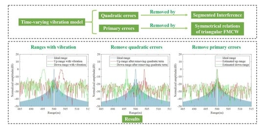
Therefore, the objective of this paper is to compensate for time-varying vibration errors by using only one-period signals without adding additional hardware. To achieve this goal, we first give an analysis of the vibration influence on the range measurement of FMCW LiDAR signals and then propose a time-varying vibration compensation method by using segmented interference. In this method, we divide the time-varying vibration errors into primary errors caused by the constant vibration velocity and quadratic errors. The quadratic vibration errors are removed by the segmented interference method, and the primary vibration errors are compensated by establishing symmetrical mathematical relations of one-period triangular FMCW signals. We verify the effectiveness of the proposed method and its superiority over traditional methods by simulation tests of point target and 3D target. Compared with traditional methods, the advantages of the proposed method include: (1) it can compensate for not only the errors with constant vibration velocity but also time-varying vibration errors without changing the system design; (2) it uses only one-period dechirp signals, which meets the requirement of 3D scanning image; (3) it adopts coherent accumulation in the frequency domain, making it robust to noise.
2. Time-varying Vibrations in FMCW LiDAR Signals
Figure 1 represents the system design of triangular FMCW coherent LiDAR. The waveform of the transmitted signal is triangular FMCW that is generated by a tunable laser, and the transmitted signal is then divided into two signals through coupler 1. One signal separated by coupler 1 serves as a local oscillator signal, and the other signal serves as a transmitted signal that is emitted by an optical antenna. Then, the transmitted signal is reflected when a target is encountered and passes through a circulator. Next, the local oscillator signal separated by coupler 1 travels through a delay fiber, which is then mixed with the echo signal reflected from a target through coupler 2. The mixed signal is coherently detected by detector DM [17]. At last, a digital acquisition card DAQ is used to sample the dechirp signals, and the data is sent to the computer for subsequent signal processing [18,19]. The coherently detected signals are called dechirp signals in the following part.
The up observation of a triangular FMCW period is taken as an example to derive the influence of time-varying vibration errors on ranging. The ideal transmitted signal is a linear frequency modulation signal, which can be expressed as:
where is the transmitted signal; is the envelope of the transmitted signal; is the initial frequency of the tunable laser, and is the frequency modulation rate.
The echo signal reflected by a target at range can be expressed as:
where is the received signal at range ; is the velocity of laser, and is the delay time of the echo signal.
Then, we coherently interfere with the transmitted signal and the echo signal and obtain the dechirp signal that is represented as:
where is the dechirp signal; * is the conjugate process, and the envelope will be ignored in the following part. The term of the above equation represents the residual video phase (RVP) introduced by the dechirp process, which can be removed by using an RVP filter in the frequency domain. The RVP filter is expressed as:
After removing RVP from Equation (3) by using the RVP filter, the dechirp signal shown in Equation (3) is now simplified as:
By applying Fourier transform to the above equation, we can obtain the frequency spectrum:
where represents the signal period. The frequency spectrum is converted into the range of target:
where is the theoretical dechirp frequency at range without vibrations.
The above equations are correct when the relative range between the LiDAR platform and the target is constant. For a vibrating LiDAR platform, the range of target can be expressed as second-order Taylor expansion [13,14]:
where is the time-varying range in a vibrated environment, and is the initial velocity and acceleration of vibration, respectively. We should note that the sine function is more realistic to describe the vibration of the lidar platform in the whole observation process if the vibration is particularly regular. In this case, the local sinusoidal vibration can be approximated as a polynomial form when the vibration period is much larger than the signal period. According to References [13,14], the vibration in a one-period signal can be expressed as the quadratic function. Thus, we use the quadratic function to approximate the vibration in a one-period signal. Then, the dechirp signals containing time-varying vibration errors can be expressed as [20]:
In the above equation, the maximum range error introduced by cubic term within a period can be approximated to:
where is the dechirp frequency introduced by cubic term in Equation (9). As is on the order of microseconds or milliseconds, the range error introduced by cubic term can be ignored. Thus, the dechirp signal containing vibration errors can be simplified as:
The dechirp signal with vibration errors in the above equation can be regarded as a signal with linear frequency modulation, whose initial frequency is the primary coefficient and the modulation frequency rate is which is twice the quadratic coefficient. In the following part, and are denoted as the quadratic vibration error and the primary vibration error, respectively. The vibration displacement is usually magnified thousands of times because the laser wavelength is short, and the primary vibration errors will cause a great deviation of the ranging results. In addition, the quadratic vibration errors and noise will cause spectrum broadening. In the case of high SNR, the quadratic vibration errors are mainly responsible for the main lobe broadening. The scattering point of a target range will spread to the adjacent range gate, making the one-dimensional range distributions blurred. Therefore, the existence of time-varying vibration errors defocuses the imaging result and yields a large error to the ranging result, and it is necessary to reduce the effect of time-varying vibrations to improve ranging performance.
3. Time-varying Vibration Compensation Based on Segmented Interference
Triangular FMCW is used as the transmitted signal, and the up dechirp signal and down dechirp signal are obtained by coherent detection. Then the dechirp signals containing time-varying vibration errors are respectively expressed as:
where and represent the up and down dechirp signals in a triangular frequency modulation period, respectively; and are the center time of up and down observations in one-period FMCW signal, respectively. The above equation can be abbreviated as follows:
where ,, and are the constant term, the primary coefficient and the quadratic coefficient in the phase of , respectively; , and are the constant term, the primary coefficient and the quadratic coefficient in the phase of , respectively. Then, we will introduce the quadratic vibration error and primary vibration error compensation methods, respectively.
3.1. Compensate for the Quadratic Vibration Errors
In this section, a segmented interference method is used to compensate for the quadratic vibration errors of the dechirp signals. The up and down dechirp signals in Equation (13) are first derived into two segmented dechirp signals by half and half, and the segments are not overlapping. The up segmented dechirp signals and the down segmented dechirp signals can be denoted as:
where and are segmented signals of up dechirp signal with a center time of and , respectively; and are segmented signals of down dechirp signal with a center time of and , respectively. Then, the up interference signal is obtained by interfering and , and the down interference signal is obtained by interfering and . The interference signals are shown as:
where and are the up and down interference signals, respectively. The interference signals in Equation (15) are single-frequency signals. Then, we apply Fourier transform to the interference signals, and the frequencies of up and down interference signals can be expressed as:
where and are the interference frequencies of up and down interference signals, respectively. The quadratic coefficients of up and down dechirp signals can be obtained:
where and are the estimated quadratic coefficient, respectively. The quadratic vibration compensation filters can be designed by using the estimated coefficients, which are shown as:
where and are the quadratic vibration compensation filters of up and down observations, respectively. Then, and are used to remove the quadratic vibration errors shown in Equation (12). The dechirp signals after removing quadratic vibration errors are shown as:
where and are the up and down dechirp signals after compensating for the quadratic vibration errors, respectively.
3.2. Compensate for the Primary Vibration Errors
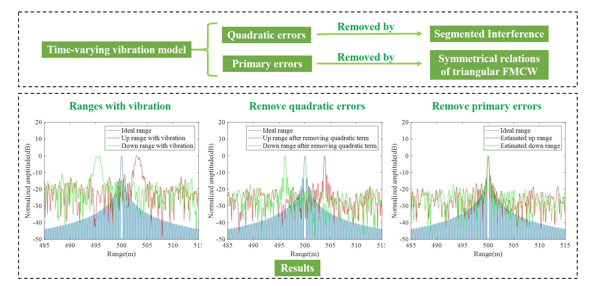
Figure 2 shows the schematic diagram of triangular FMCW ranging with primary vibration errors. The green line represents the ideal transmitted frequency, and the red dashed line represents the received echo that contains primary vibration errors. Then, we use blue solid lines to denote the dechirp frequency containing primary vibration errors and represent the Doppler frequency introduced by primary vibration errors. The Doppler frequency in the up and down dechirp signals can be estimated by using the symmetrical relations of the spectrums of the up and down dechirp signals. Then the primary vibration errors can be calculated by using the estimated Doppler frequency.
In Equation (19), the dechirp signals after removing the quadratic vibration errors are single-frequency signals, and there is no obvious spectrum spread in the one-dimensional range distributions, making the spectrum peak clearly discernable. Therefore, Fourier transform is performed on the up and down dechirp signals in Equation (19), and the frequencies corresponding to the spectrum peaks are the dechirp frequencies containing only primary vibration errors. The dechirp frequencies of the up and down dechirp signals can be respectively expressed as:
where is the dechirp frequency corresponding to the ideal range of the target, and is the Doppler frequency introduced by the primary vibration errors. According to the principle of Doppler effect, the relationship between Doppler frequency and velocity can be expressed as:
The initial vibration velocity can be estimated by using Equations (20) and (21):
where is the estimated initial velocity. The estimated initial velocity is then used to design the primary vibration compensation filters that can be expressed as:
The above filters are used to compensate for the primary vibration errors of the dechirp signals. Then, the up and down dechirp signals after compensating for primary vibration errors can be respectively expressed as:
At last, Fourier transform is applied to Equation (24) to estimate the actual range of target after removing the vibration errors.
3.3. Process Flow of the Proposed Vibration Compensation method
This section introduces the process flow of the proposed time-varying vibration compensation method by using segmented interference. First, the dechirp signal of one triangular FMCW period is divided into up and down dechirp signals which are then divided into two segmented dechirp signals, respectively. Second, the quadratic vibration coefficients are estimated by segmented interference of the segmented dechirp signals, and then quadratic compensation filters are established to remove the quadratic vibrations from the original dechirp signals. Finally, the primary vibration errors are estimated by using the symmetrical mathematical relations of the dechirp signals in one triangular FMCW period, and the primary compensation filters are designed to remove the primary vibrations introduced by constant vibration velocity. The process flow of the proposed time-varying vibration compensation method by using segmented interference is shown in Table 1.
In Table 1, the symbol j is used to denote the directions of frequency sweep, namely, the dechirp signals and the dechirp frequencies of up and down observations in a triangular FMCW period. To be specific, j = 1 represents the corresponding data of up observation and j = 2 represents the corresponding data of down observation.
4. Experimental Analysis
We use five experiments to verify the effectiveness of the proposed vibration compensation method in compensating for time-varying vibrations and the advantages of the proposed method compared with traditional vibration compensation methods. The first and second experiments are designed to verify the adaptiveness of this method under the environments of constant vibrations and time-varying vibrations, respectively. The third experiment is designed to show the validity of the proposed method in dealing with different vibration parameters. The fourth experiment is a multi-component target test, and the fifth experiment is a 3D imaging test. We list the parameters of the LiDAR system in Table 2.
4.1. Constant Vibration Test
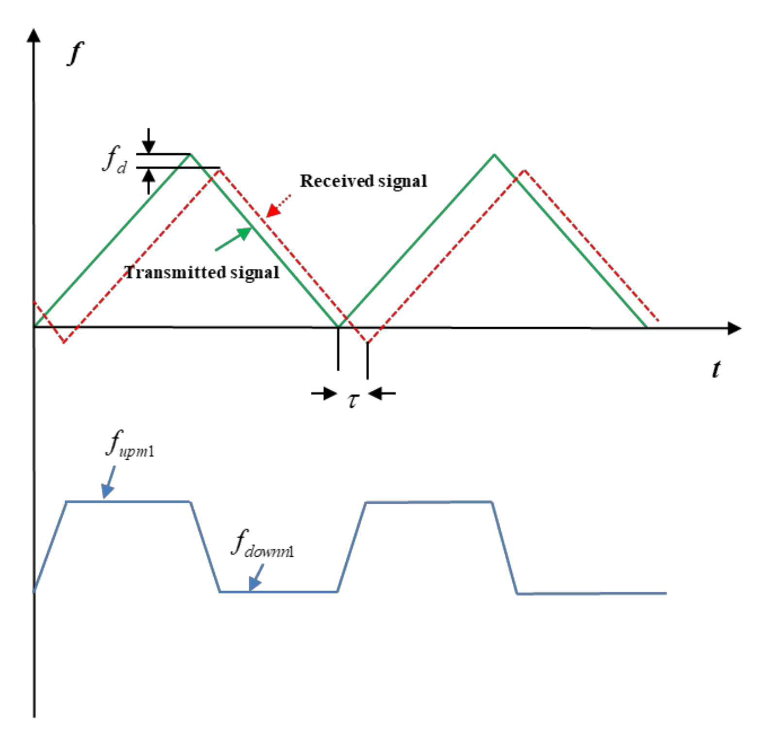
To prove the applicability of the proposed method under the condition of constant vibration velocity, we added a vibration with a velocity of 0.02 m/s to the LiDAR movement. Figure 3a shows the real parts of the ideal dechirp signal, the up and down dechirp signals containing vibration errors, respectively. Figure 3b,c show the vibration errors and the vibration velocities of the up and down observations. Figure 3c shows that the lidar moves with a constant vibration velocity during the signal acquisition. Since the vibration velocity shown in Figure 3c is constant, the vibration errors shown in Figure 3b vary linearly towards time. Then we applied Fourier transform to the signals shown in Figure 3a, and the frequency spectrums were then converted to range distributions, after which we obtain the range distributions of dechirp signals, as shown in Figure 3d. The ideal range is represented by the peak of the blue curve (500 m). Figure 3d shows that the peak of the red curve is much larger than the actual range of the target, while that of the green curve is much smaller than the actual range of the target. This phenomenon shows the influence of Doppler frequency shift on ranging, as described by Equation (11). Then, we use the proposed vibration compensation method to extract the actual range.
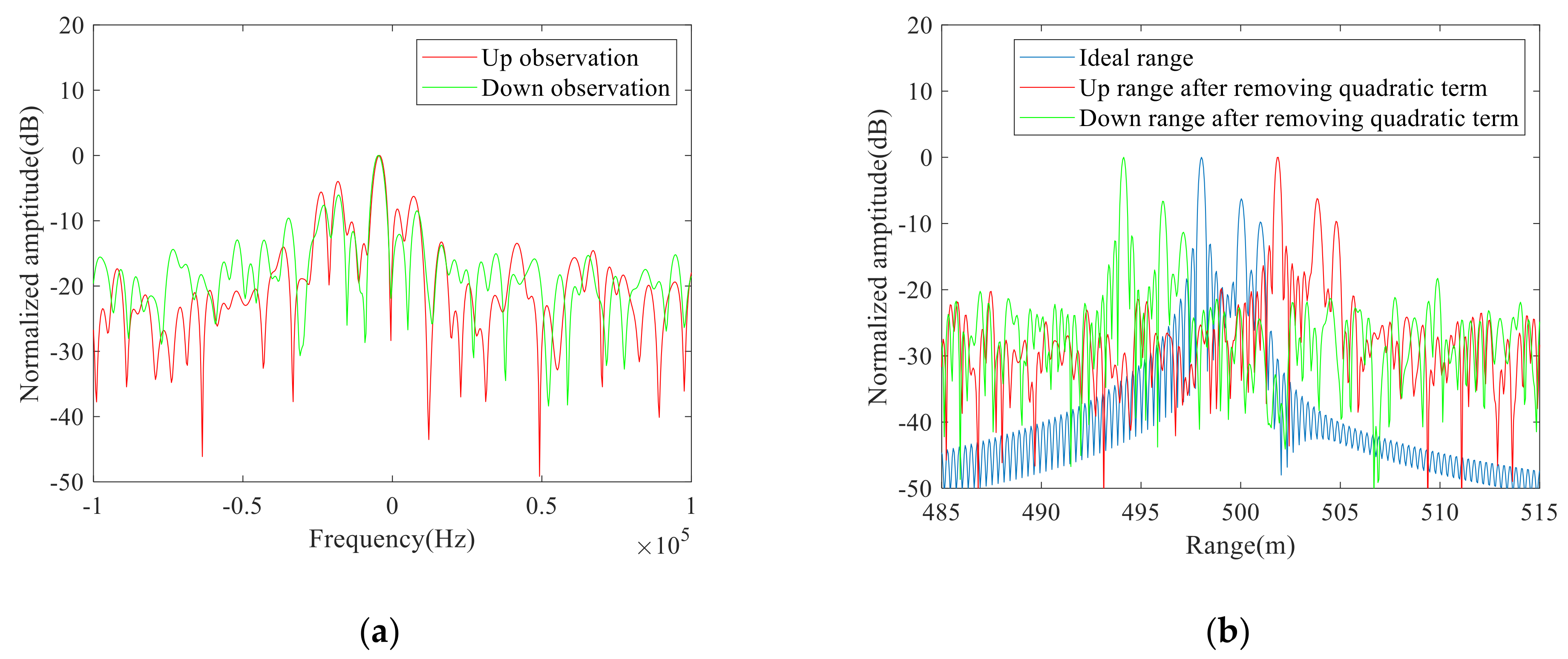
First, the segmented interference method is used to remove the quadratic vibrations in the original dechirp signals. Figure 4a shows the interference frequencies of the up and down observations after segmented interference by using Equation (15), and the quadratic coefficients of up and down dechirp signals can be estimated by using the peak frequencies. According to the estimated quadratic coefficients, we designed quadratic compensation filters that are used to remove quadratic vibrations from the original dechirp signals, respectively. Then, we applied Fourier transform to the signals after compensating for quadratic vibration errors, and the one-dimensional range distributions of the dechirp signals are depicted in Figure 4b. As the vibration velocity is constant, the quadratic vibration errors do not exist. Therefore, the range distributions after quadratic compensation as shown in Figure 4b are consistent with that before quadratic compensation as shown in Figure 3c.
Then, the symmetrical relations of triangular FMCW are used to remove the primary vibrations. The up and down dechirp signals after compensating for quadratic errors are converted to frequency spectrums, and the peaks of the frequency spectrums were regarded as the dechirp frequencies containing only primary errors. Then the initial vibration velocity can be estimated by using the mathematical relations of triangular FMCW signals, which were used to design primary compensation filters and thereby remove the primary errors. Moreover, the corresponding range distributions are depicted in Figure 4c. Compared with Figure 3c, the range was extracted to be 500 m by selecting the peak of the red curve in Figure 4c, which is consistent with the theoretical value (500 m). Thus, the proposed method is effective to remove the errors introduced by constant vibration.
As the Doppler frequency shift method proposed in Reference [16] and the three-point method proposed in Reference [15] can also use an only one-period signal to compensate for vibration errors, these two methods were used to compare with the proposed method in dealing with the dechirp signals in Figure 3a. The range distributions obtained by the Doppler frequency shift method are depicted in Figure 4d. The peak range (500 m) of the red curve is regarded as the estimated range, which is consistent with the theoretical value. Thus, the Doppler frequency shift method is useful to estimate the actual range on the condition of constant vibration. The phases in the up and down observations are depicted in Figure 4e, and we calculated the range of the target to be 499.93 m by using the three-point method, which is close to the theoretical value. Therefore, all three methods can achieve good vibration compensation results under the condition of constant vibrations.
4.2. Time-Varying Vibration Test
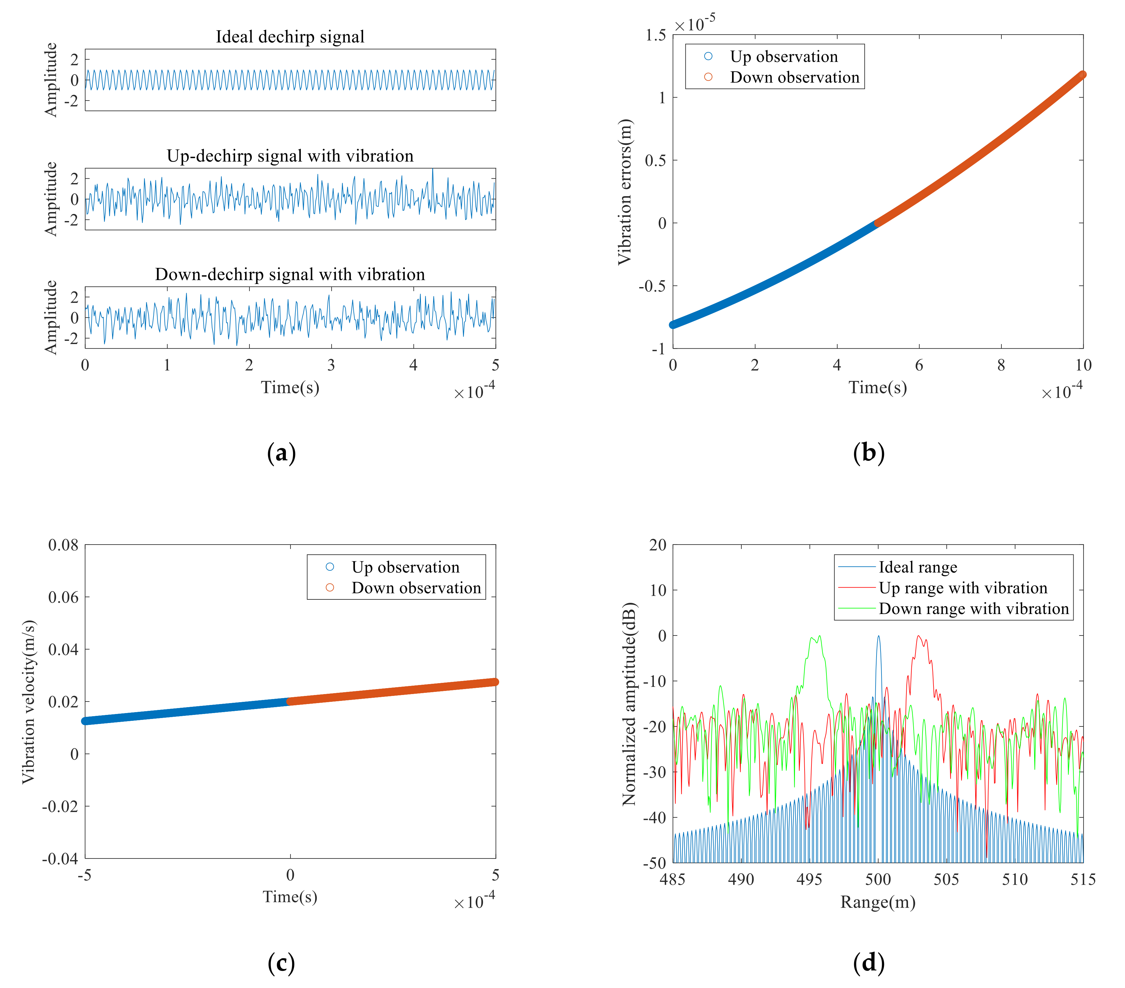
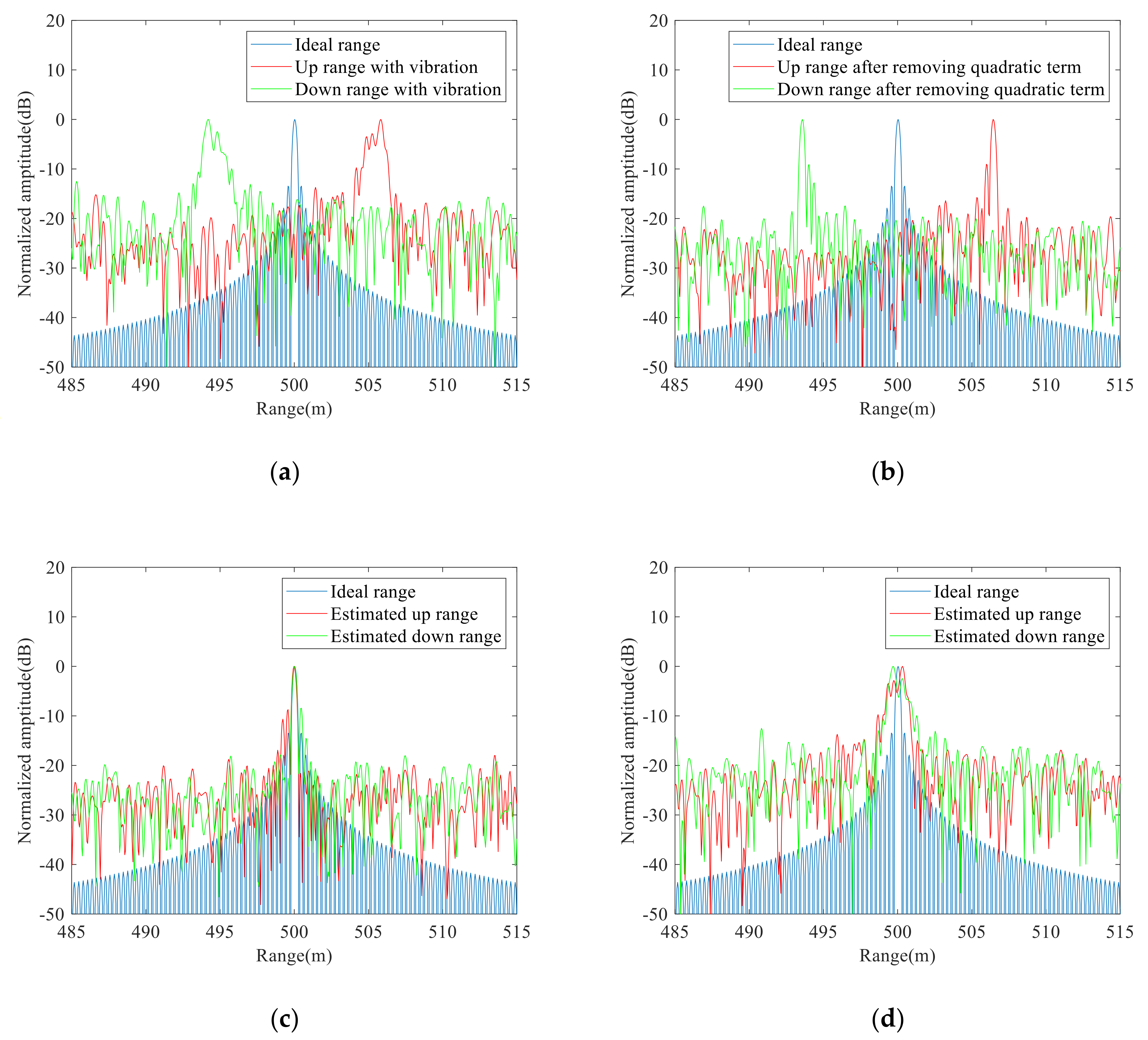
To prove the effectiveness of the proposed vibration compensation method under the condition of time-varying vibration, we added a vibration with a velocity of 0.02 m/s and an acceleration of 15 m/s2 to the LiDAR movement. Further, Gaussian white noise with a signal-to-noise ratio (SNR) of 0 dB was added to the ideal signals to test the adaptability of the proposed method to noise. Figure 5a is the real parts of the clean dechirp signal, the up and down dechirp signals with time-varying vibration errors and noise, respectively. Figure 5b, c show the vibration errors and the vibration velocities of the up and down observations. Figure 5c shows that the LiDAR moves with a constant acceleration during the signal acquisition. Due to the influence of acceleration, the vibration errors are quadratically varying related to time. Fourier transform was carried out for the dechirp signals in Figure 5a, and the frequency spectrums were then converted into range distributions, as shown in Figure 5d. The peak of the blue curve in Figure 5d represents the ideal range to be 500 m. Figure 5d indicated that the time-varying vibration errors greatly reduce the range resolution, and the quadratic errors and noise cause spectrum broadening. If we directly extract the peak of the red curve as the actual range, the ranging results will have great deviations.
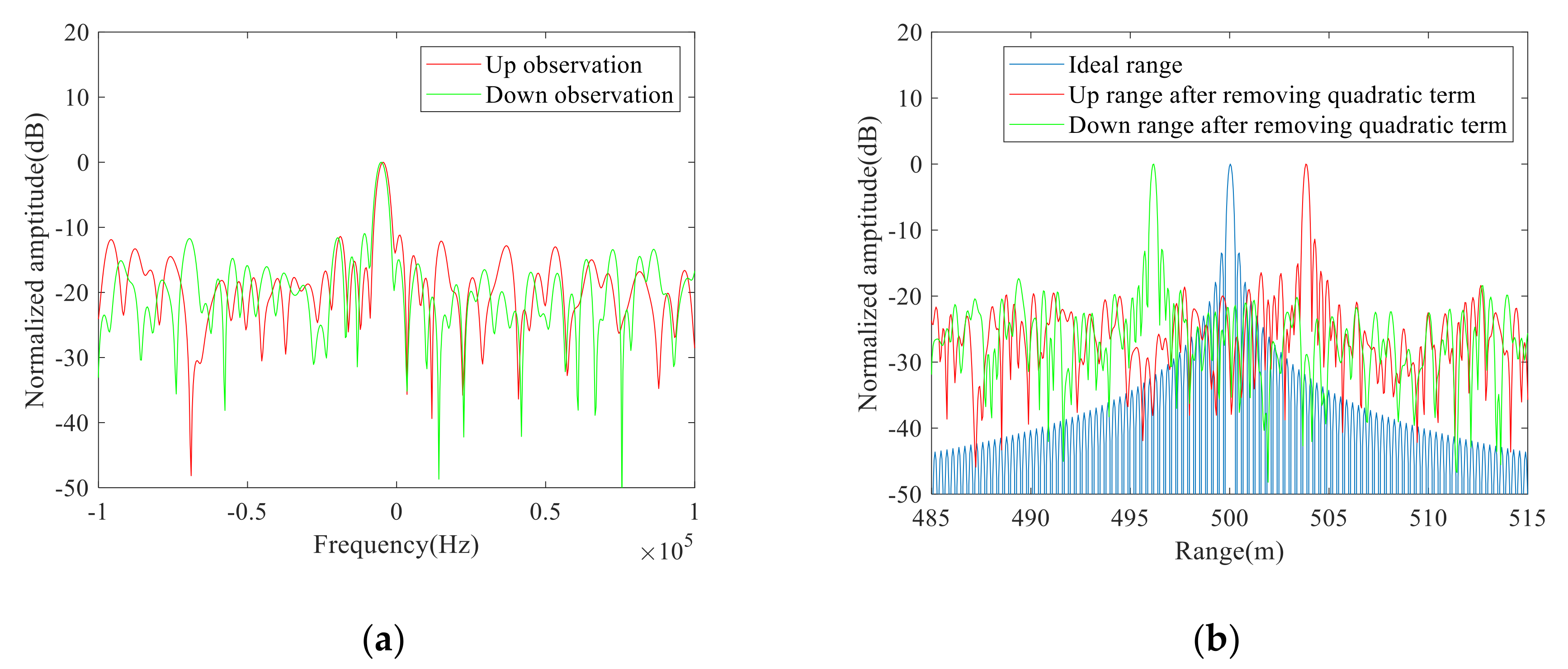
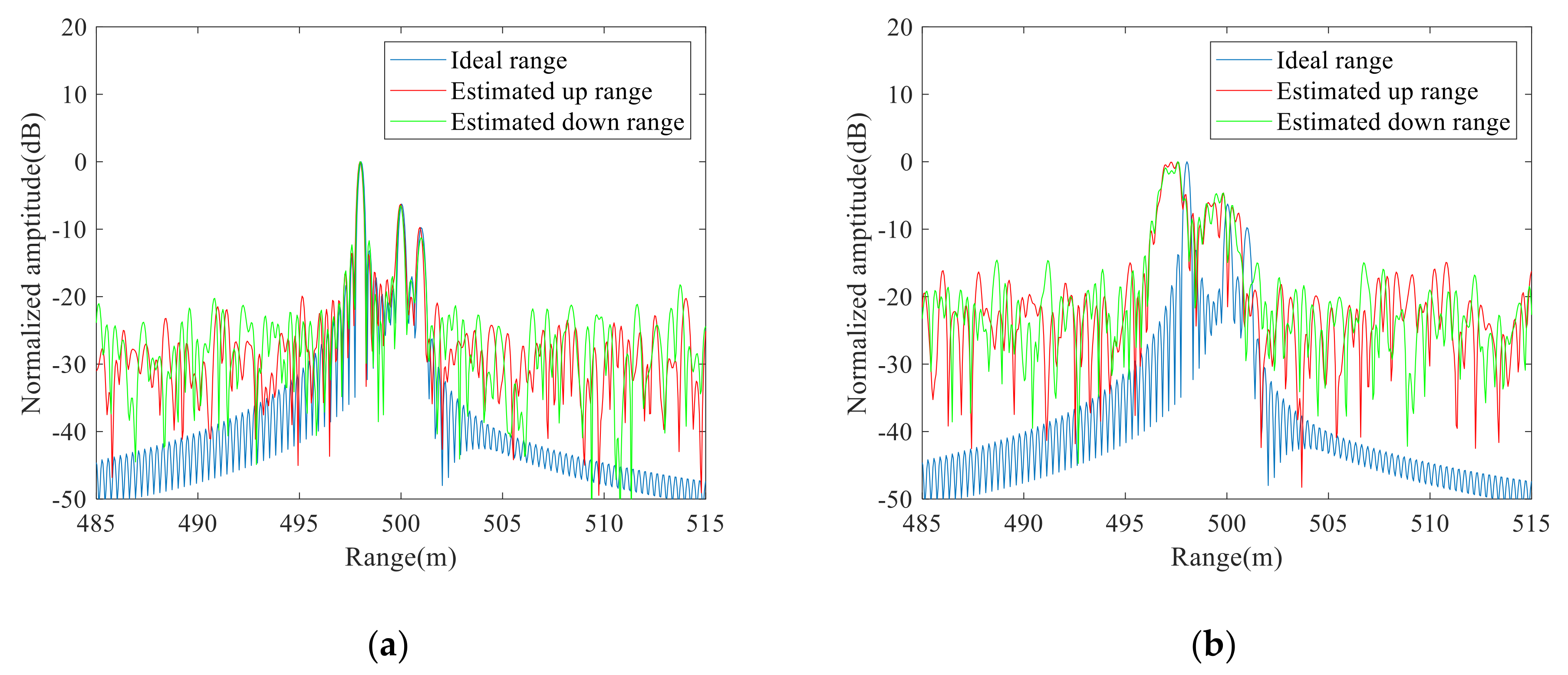
The proposed method was used to eliminate the time-varying vibration errors. First, we used the segmented interference method to remove the quadratic vibration errors. Figure 6a shows the interference frequencies of the up and down observations. By extracting the peak frequencies, we estimated the quadratic coefficients which were then used to design quadratic compensation filters to compensate for the quadratic vibration errors in Figure 5a. The one-dimensional range distributions after compensating for quadratic vibration errors were shown in Figure 6b. Compared with Figure 5c, the spectral energy in Figure 6b is more concentrated, and the peak ranges of the up and down observations are symmetrically distributed around the theoretical range of the target. Then, we used the symmetrical relations of triangular FMCW to remove the primary vibration errors, and the one-dimensional range distributions are depicted in Figure 7a. As shown in Figure 7a, the peak of the red curve was extracted to be 500 m that is consistent with the theoretical value, which indicates that this method can effectively estimate the actual range under the condition of time-varying vibrations.
For comparison, the Doppler frequency shift method proposed in Reference [16] and the three-point method proposed in Reference [15] were also used to compensate for the time-varying vibration errors of the dechirp signals in Figure 5a. The one-dimensional range distributions obtained by the Doppler frequency shift method are shown in Figure 7b. Compared with Figure 5c, the peak ranges in Figure 7b are closer to the theoretical value, but the spectrum broadening introduced by quadratic errors and noise is not solved. Figure 7b shows that the estimated range was 499.5 m that is smaller than the ideal range. Then, we applied the three-point method to the signals in Figure 5a, and the phases in the up and down observations are shown in Figure 7c. As noise affects the accuracy of phase unwrapping, the range was calculated to be 498.73 m that is quite different from the theoretical value (500 m). Therefore, the range measurement results of the proposed method are more accurate than those of the traditional methods under the environment of time-varying vibrations and noise.
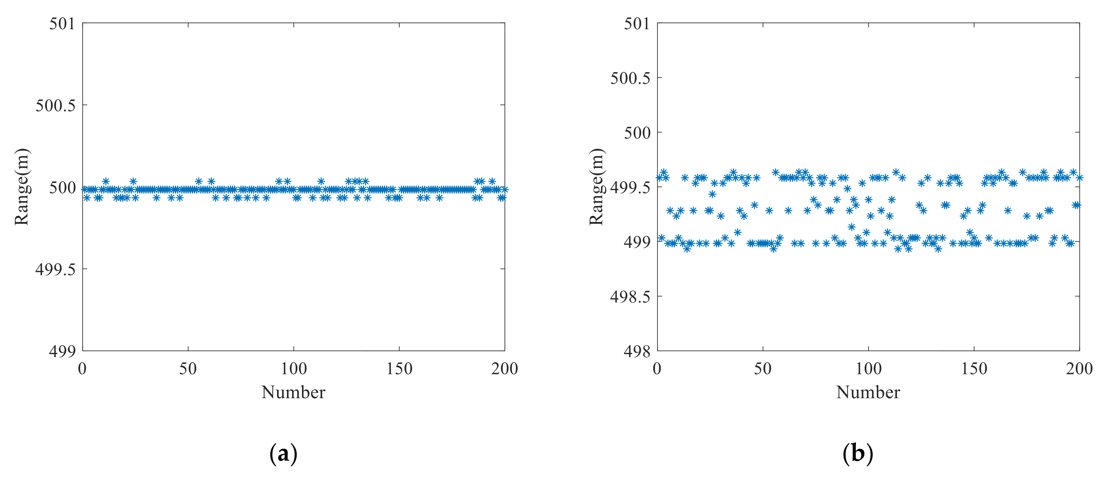
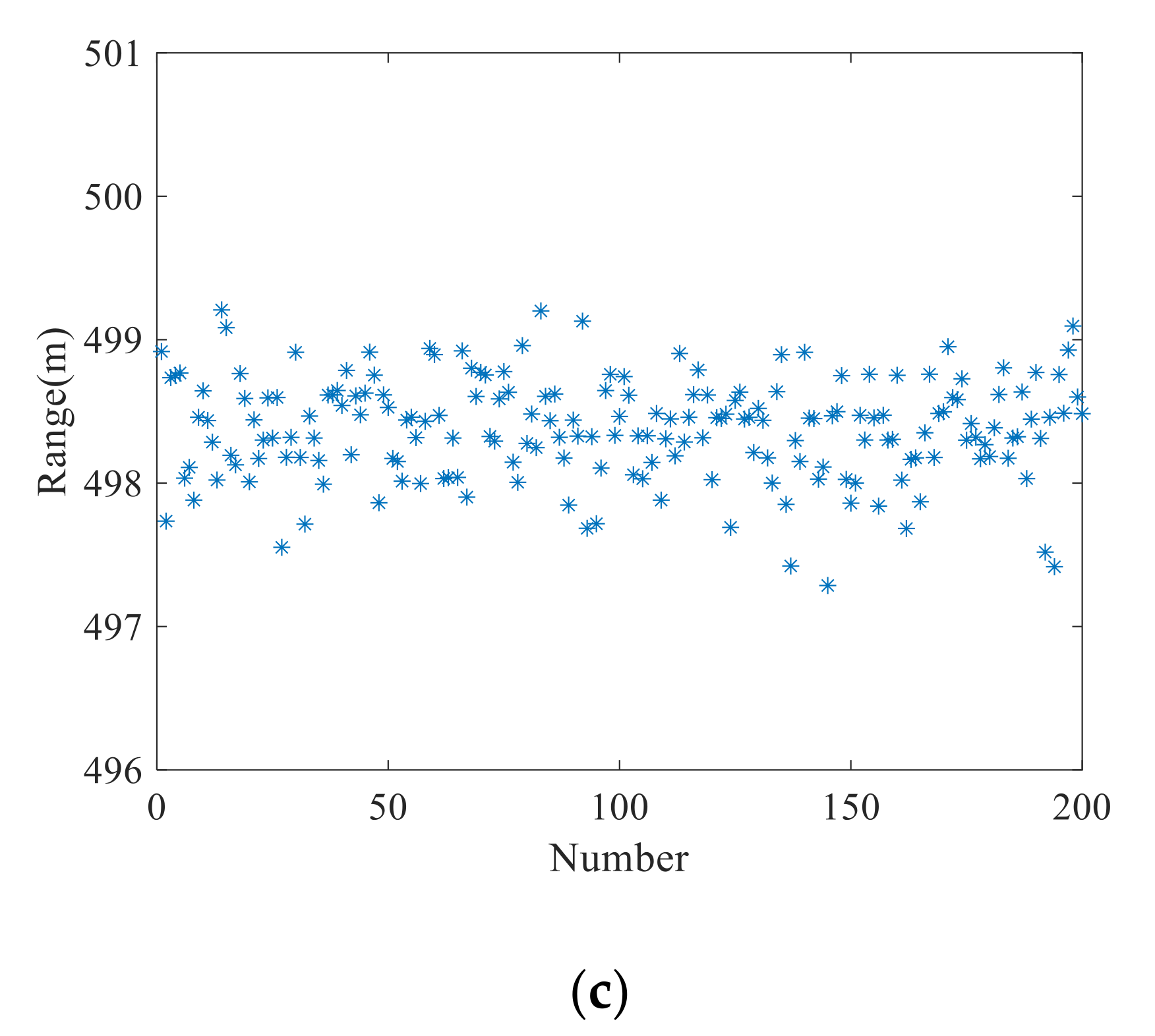
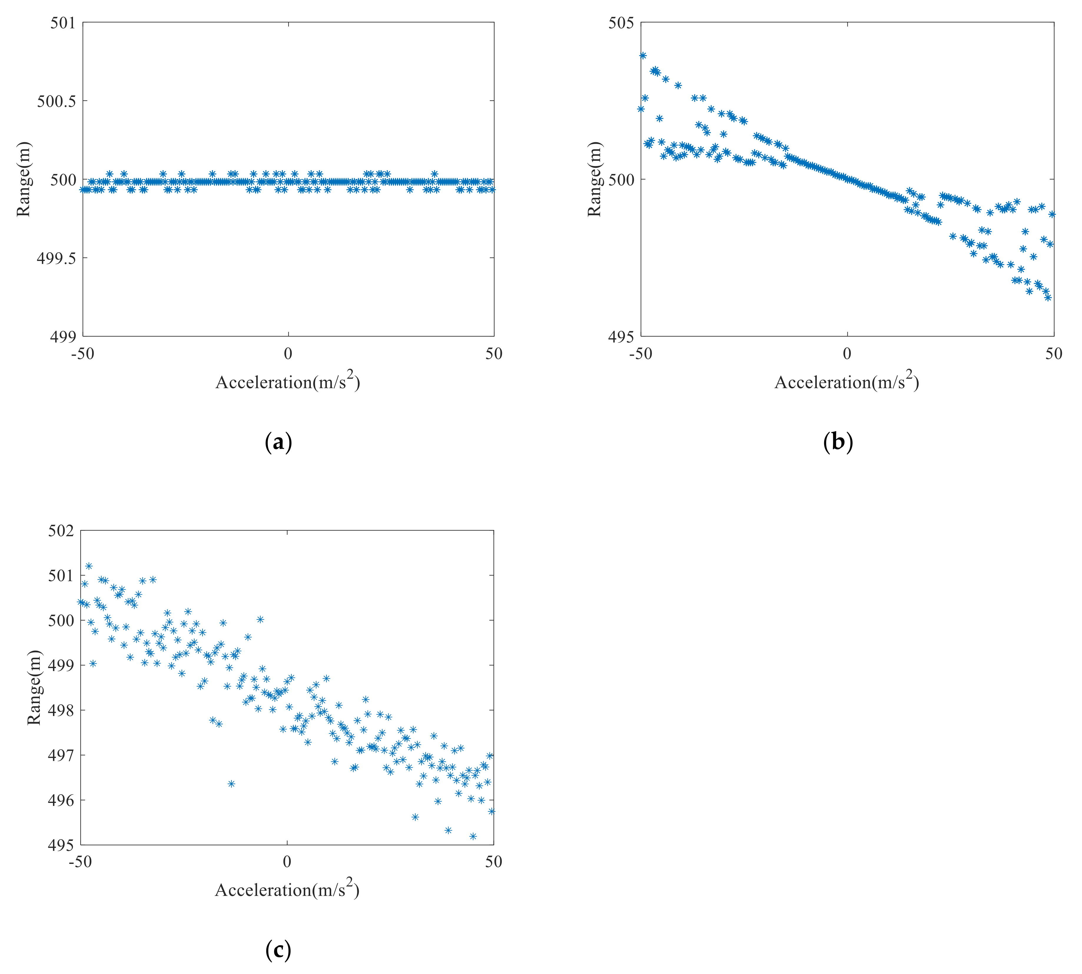
To demonstrate the robustness of the proposed method and its advantages over the other traditional vibration compensation methods, we repeated the above test 200 times, and the range measurement results are shown in Figure 8. To give quantitative evaluations of the ranging results, we calculated the root mean square errors (RMSE) [21] and mean values of the ranging results in Figure 8. The RMSE and mean value obtained by the proposed method shown in Figure 8a are 0.03 m and 499.98 m, respectively. The RMSE and mean value obtained by the Doppler frequency shift method shown in Figure 8b are 0.79 m and 499.25 m, respectively. Moreover, the RMSE and mean value obtained by the three-point method shown in Figure 8c are 1.67 m and 498.36 m, respectively. As the three-point method only uses three phase points to establish mathematical relations and then estimate the actual range, the random noise inevitably introduces jitter to the specific points which will seriously affect the ranging results. The proposed vibration compensation method and Doppler frequency shift method can effectively eliminate the influence of noise on ranging results through a coherent accumulation process in the frequency domain. Therefore, the two methods are more robust to noise than the three-point method which uses only three phase points. However, as the Doppler frequency shift method uses the relative frequency shift between the up and down observations to estimate the vibration errors and thereby compensates for the vibration errors, it can only eliminate the vibrations introduced by constant velocity but cannot eliminate the quadratic vibration errors. Therefore, compared with the traditional vibration compensation methods, the proposed method can obtain more accurate estimation results when dealing with time-varying vibration errors.
4.3. Test for Different Vibration Parameters
This subsection will test the superiority of the proposed vibration compensation method over the traditional methods under environments with different vibration parameters. We first added a vibration with velocity of 0.02 m/s and different accelerations (−50 m/s2~50 m/s2) to the LiDAR movement. Then, we added noise with SNR of 0 dB to the dechirp signals with vibration errors.
The proposed method, the Doppler frequency shift method and three-point method were used to estimate the actual range (500 m), and the range measurement results are shown in Figure 9a–c. As shown in Figure 9a, the ranging errors obtained by the proposed method rarely change with the increase of acceleration, and the range measurement results are all close to the ideal range of the target. As the proposed method can simultaneously remove the quadratic vibration errors and the primary vibration errors introduced by the constant vibration velocity, the measurement results of the proposed method are stable and accurate. As shown in Figure 9b, the ranging results of the Doppler frequency shift method have small errors when the acceleration is around 0 m/s2. With the increase of the absolute value of acceleration, the ranging results seriously deviate from the theoretical value. As the Doppler frequency shift method only considers the frequency shift introduced by the constant vibration velocity, this method can only estimate and remove the primary vibration errors. As shown in Figure 9c, the ranging results of the three-point method are unstable, and the result even have large errors under the condition of constant vibration velocity because of noise. Therefore, the proposed method is more stable and robust than the traditional vibration compensation methods under the environments of time-varying vibration errors and noise.
We also carried out an experiment to show the superiority of the proposed method in dealing with a sine-wave movement. Sinusoidal vibrations were added to the LiDAR movement and the amplitude and frequency are 20 μm and 250 Hz, respectively. Then, a noise with an SNR of 0 dB was superimposed into the dechirp signals simultaneously. Figure 10a shows the one-dimensional range distributions with sine-wave vibration errors. The time-varying vibration errors greatly reduce the range resolution, and the main lobes of the range distributions are broadening.
The proposed method was used to eliminate the time-varying vibration errors. The one-dimensional range distributions after compensating for quadratic vibration errors and the primary vibration errors are shown in Figure 10b,c, respectively. As shown in Figure 10c, the peak of the red curve was extracted to be 500 m, which is consistent with the theoretical value, which indicates that the proposed method can effectively estimate the actual range under the condition of sine-wave vibrations. For comparison, the Doppler frequency shift method was also used to compensate for the sine-wave vibration errors. The one-dimensional range distributions obtained by the Doppler frequency shift method are shown in Figure 10d. Figure 10d shows that the problem of spectral broadening is not solved, and the estimated range was 500.2 m that is bigger than the ideal range. Therefore, compared with the Doppler frequency shift method, the proposed method can obtain more accurate results when dealing with sine-wave vibration errors.
4.4. Test for Multi-component Target
This subsection will test the applicability of the proposed vibration compensation method to deal with multi-component targets, we constructed three-point targets with ranges of [498 m, 500 m, 501 m]. A vibration with a velocity of 0.02 m/s and an acceleration of 15 m/s2 was added to the LiDAR movement and we also added noise with an SNR of 0 dB to the ideal dechirp signal. Figure 11a shows the real parts of the ideal dechirp signal, the up and down dechirp signals with time-varying vibration errors, respectively. The range distributions are shown in Figure 11b. Figure 11b shows that the time-varying vibration errors broaden the spectrums, and it is hard to accurately identify three ranges.
Then the proposed method was used to remove the time-varying errors of the dechirp signals. Figure 12a shows the interference frequencies of the up and down observations after segmented interference. Since the vibrations of all points in one observation spot are the same, we just need to extract the frequencies that correspond to one clearer point. By using the extracted frequencies, we can compensate for the vibrations of all the points. According to the interference frequencies, we designed quadratic compensation filters of the up and down observations, by using them we can eliminate the quadratic errors. The one-dimensional range distributions after removing quadratic vibration errors are shown in Figure 12b. The spectrum energy in Figure 12b is more concentrated compared with that in Figure 11b, and we can clearly identify the three points. Then, we estimated the initial vibration velocity by using the triangular symmetric relations of up and down dechirp frequencies. According to the estimated velocity, we constructed the primary compensation filters that were then used on the up and down dechirp signals, respectively. The one-dimensional range distributions after removing the primary errors are shown in Figure 13a. We extracted three ranges to be [498 m, 499.99 m and 501.02 m] from Figure 13a, which are close to the theoretical values. Thus, this method can effectively eliminate the vibration errors and thereby accurately estimate the ranges of multi-component targets.
As the three-point method is only suitable for a single-component target, only the Doppler frequency shift method was used as a contrast to remove the vibrations of the dechirp signals in Figure 11a, and we obtained the range distributions, as shown in Figure 13b. Compared with Figure 11b, the overall ranges in Figure 13b are closer to the theoretical values, but they still suffer from spectrum broadening. As the Doppler frequency shift method performs well when the vibration is stable, it cannot eliminate the quadratic vibration errors. As shown in Figure 13b, it is difficult to directly identify the ranges of multi-component targets. Therefore, this test verifies the superiority of the proposed method in dealing with multi-component targets under the condition of time-varying vibration errors.
4.5. 3D Imaging Test
This subsection applied the proposed method to a 3D scene to verify its applicability to 3D imaging. The workflow of the 3D data process is as follows. First, the LiDAR system collects the dechirp signal from one observation spot and then calculates the corresponding range of this spot. Combined with the navigation information and scanning angle of the LiDAR platform, we can estimate the height of the target in this observation spot. Thus, the 3D scene of interest can be reconstructed by 3D scanning. We constructed an ideal 3D scene for comparison which is shown in Figure 14a. Then, the simulation parameters were applied to the 3D scene in Figure 13a to obtain the ideal 1D dechirp signals of each observation spot. Sinusoidal vibrations were added to the LiDAR movement and the amplitude and frequency are 30 μm and 80 Hz, respectively. Then, a noise with SNR of 2 dB was superimposed into the dechirp signals simultaneously. To show the impact of vibrations on 3D imaging, we applied Fourier transform to the collected signals of each observation spot, and the 3D imaging result was obtained by taking the peak range as the range of this observation spot, as shown in Figure 14b. The 3D imaging result in Figure 14b deviates from the ideal imaging result in Figure 14a when the dechirp signals contain vibration errors, affecting the subsequent target recognition and the acquisition of ground elevation.
The proposed method was performed on each observation spot, and the corresponding 3D imaging results are shown in Figure 15a. The difference between the reconstructed 3D imaging result and the ideal one is shown in Figure 15b. Figure 14 and Figure 15 show that most of the vibration errors were removed, and the fluctuation trend of the reconstructed result is close to the ideal one. For comparison, the Doppler frequency shift method was also used in the 3D structure, and the reconstructed result is shown in Figure 16a. The reconstruction error of the Doppler frequency shift method is shown in Figure 16b. Figure 16b indicates that the reconstructed 3D result after using the Doppler frequency shift method has minor deformation compared with the ideal one. This is because it only considers the influence of constant vibration velocity and ignores the influence of quadratic vibration errors. Therefore, the 3D imaging result obtained by the proposed method in Figure 15b is closer to the ideal 3D imaging result than that obtained by the Doppler frequency shift method. To give a quantitative analysis, we calculated the RMSEs of the proposed method and the Doppler frequency shift method, and the results are 0.04 m, and 0.13 m, respectively. Therefore, the proposed method can obtain more stable and accurate 3D imaging results compared with the Doppler frequency shift method, which indicates that the proposed vibration compensation method has superiority in compensating for the time-varying vibration errors of the 3D structure.
5. Discussion
Studies [10,11,12] used multiple lasers or additional hardware devices to compensate for vibration errors and thereby achieve accurate ranging results. However, multiple lasers may introduce asynchronous problems and increase costs. Compared with [10,11,12], the proposed method does not need additional lasers and avoids the asynchronous problem between multiple lasers, which reduces the hardware configuration. Tao et al. [13,14] needed long-time observed data to eliminate the vibrations. However, a 3D imaging system uses a laser scanner to dynamically measure the range of the target, and the observation time of one laser spot is short, which does not meet the requirements of the above methods. To solve the above problems, the dechirp signal of one triangular FMCW period is firstly divided into up and down dechirp signals, and then the up and down dechirp signals are divided into segmented dechirp signals, respectively. Compared with [13,14], the proposed method only needs one-period signals to compensate for the time-varying vibration errors, which is suitable for 3D imaging.
The three-point method [15] selects three phase points from one-period signals to establish mathematical relations and thereby remove the errors introduced by constant vibration velocity, but the jitters introduced by random noise will affect the phase unwrapping and the ranging accuracy. However, the proposed method adopts coherent accumulation in the frequency domain, which can effectively eliminate the influence of noise on ranging. The Doppler frequency shift method [16] can use one-period signals to estimate and thereby eliminate the relative frequency shift, which achieves excellent results under the condition of constant vibration velocity. However, the vibration velocity is time-varying, which degrades the accuracy of range measurements of this method. To solve the above problems, the segmented interference is first used in the proposed method to estimate and eliminate the quadratic vibrations, following which the symmetrical mathematical relations of up and down signals are used to remove the primary vibrations. Therefore, the time-varying vibration errors can be effectively compensated by the proposed method.
When we establish the time-varying vibration model, the range of the target is approximated by a second-order Taylor expansion, which is suitable for the scene with slowly varying vibration. To be specific, we divide the time-varying vibration errors into primary errors caused by the vibration with constant velocity and quadratic errors. However, vibration with severely time-varying acceleration can lead to not only primary and quadratic errors but also higher-order errors; therefore, the proposed method may not perform well because the approximation accuracy of the quadratic function to higher-order errors is limited. For severe vibrations, we will consider the higher-order approximation in our future research.
Synthetic aperture LiDAR (SAL) and inverse synthetic aperture LiDAR (ISAL) have attracted much attention in recent years due to their ability to achieve high-resolution imaging and accurate target recognition. However, vibration has also become a tricky issue in SAL and ISAL applications. Therefore, the application of the proposed method in SAL and ISAL is our future research direction.
6. Conclusions
We derived the influence of vibration errors on the range measurement of FMCW LiDAR signals and proposed a time-varying vibration compensation method based on segmented interference. We established a time-varying vibration model which is an extension of the constant vibration model used in the traditional vibration compensation method. According to the time-varying vibration model, we removed the quadratic vibration errors by using the segmented interference method and removed the primary vibration errors by establishing symmetrical mathematical relations of the up and down observations. Numerical experiments show that the proposed method can eliminate the influence of time-varying vibration errors on ranging and 3D imaging and accurately estimate the actual ranges. Moreover, the experiments also verify the advantage of the proposed method over the traditional vibration compensation methods in dealing with noise and time-varying vibration errors with different vibration parameters. The first advantage of the proposed method is that it can compensate for the time-varying vibration errors with only one-period triangular FMCW signals, which is extremely challenging for the traditional vibration error compensation method. The other advantages of the proposed method include that it does not need to change the hardware design of the LiDAR system and it is robust to noise. However, the results may degrade for severely time-varying vibrations because the proposed method only compensates for primary and quadratic errors, and we should consider the higher-order errors in this case.
Author Contributions
Conceptualization, M.X. and R.W.; methodology, R.W. and W.L.; validation, R.W., Z.W., and Y.W.; formal analysis, B.W.; investigation, R.W. and Y.W.; resources, B.W. and Y.W.; data curation, Z.W.; writing—original draft preparation, R.W.; writing—review and editing, R.W. and W.L.; project administration, B.W.; funding acquisition, B.W. All authors have read and agreed to the published version of the manuscript.
Funding
This research was funded by the National Natural Science Foundation of China under grant number 62073306 and the Youth Innovation Promotion Association CAS.
Data Availability Statement
The data presented in this study can be available on request from the corresponding author.
Acknowledgments
The authors would like to express their gratitude to the anonymous reviewers and the associate editor for their constructive comments on the paper.
Conflicts of Interest
The authors declare no conflict of interest.
Abbreviations
The following abbreviations are used in this manuscript:
| FMCW | Frequency modulation continuous wave |
| LiDAR | Light Detection and Ranging |
| 3D | Three dimensional |
| KF | Kalman filter |
| RMSE | Root mean square error |
| SNR | Signal-to-noise ratio |
| SAL | Synthetic aperture LiDAR |
| ISAL | inverse synthetic aperture LiDAR |
References
- Menzies, R.T. Doppler lidar atmospheric wind sensors: A comparative performance evaluation for global measurement applications from earth orbit. Appl. Opt. 1986, 25, 2546–2552. [Google Scholar] [CrossRef] [PubMed]
- Balsa-Barreiro, J.; Fritsch, D. Generation of visually aesthetic and detailed 3D models of historical cities by using laser scanning and digital photogrammetry. Digit. Appl. Archaeol. Cult. Herit. 2017, 8, 57–64. [Google Scholar] [CrossRef]
- Futatsumori, S.; Morioka, K.; Kohmura, A.; Okada, K.; Yonemoto, N. Design and Field Feasibility Evaluation of Distributed-Type 96 GHz FMCW, Millimeter-Wave Radar Based on Radio-Over-Fiber and Optical Frequency Multiplier. J. Lightwave Technol. 2016, 34, 4835–4843. [Google Scholar] [CrossRef]
- Venkatesh, S.; Sorin, W.V. Phase noise considerations in coherent optical FMCW reflectometry. J. Lightwave Technol. 1993, 11, 1694–1700. [Google Scholar] [CrossRef] [Green Version]
- Huang, H.; Xu, C.; Xia, L.; Wu, C. Moving target detection based on velocity compensation methods in a coherent continuous wave lidar. J. Eng. 2019, 20, 7065–7068. [Google Scholar] [CrossRef]
- Balsa-Barreiro, J.; Avariento, J.P.; Lerma, J.L. Airborne light detection and ranging (LiDAR) point density analysis. Sci. Res. Essays 2012, 7, 3010–3019. [Google Scholar] [CrossRef]
- Balsa-Barreiro, J.; Lerma, L.J. Empirical study of variation in lidar point density over different land covers. Int. J. Remote Sens. 2014, 35, 3372–3383. [Google Scholar] [CrossRef]
- Wang, R.; Wang, B.; Xiang, M.; Li, C.; Wang, S.; Song, C. Simultaneous Time-Varying Vibration and Nonlinearity Compensation for One-Period Triangular-FMCW Lidar Signal. Remote Sens. 2021, 13, 1731. [Google Scholar] [CrossRef]
- Wang, R.; Wang, B.; Xiang, M.; Li, C.; Wang, S. Vibration compensation method based on instantaneous ranging model for triangular FMCW ladar signals. Opt. Express 2021, 29, 15918–15939. [Google Scholar] [CrossRef]
- Kakuma, S.; Katase, Y. Frequency scanning interferometry immune to length drift using a pair of vertical-cavity surface-emitting laser diodes. Opt. Rev. 2012, 19, 376–380. [Google Scholar] [CrossRef]
- Krause, B.W.; Tiemann, B.G.; Gatt, P. Motion compensated frequency modulated continuous wave 3D coherent imaging ladar with scannerless architecture. Appl. Opt. 2012, 51, 8745–8761. [Google Scholar] [CrossRef]
- Lu, C.; Liu, G.D.; Liu, B.G.; Chen, F.; Gan, Y. Absolute distance measurement system with micro-grade measurement uncertainty and 24 m range using frequency scanning interferometry with compensation of environmental vibration. Opt. Express 2016, 24, 30215–30224. [Google Scholar] [CrossRef]
- Tao, L.; Liu, Z.; Zhang, W.; Zhou, Y. Frequency-scanning interferometry for dynamic absolute distance measurement using Kalman filter. Opt. Lett. 2014, 39, 6997–7000. [Google Scholar] [CrossRef] [PubMed]
- Jia, X.; Liu, Z.; Tao, L.; Deng, Z. Frequency-scanning interferometry using a time-varying Kalman filter for dynamic tracking measurements. Opt. Express 2017, 25, 25782–25796. [Google Scholar] [CrossRef] [PubMed]
- Swinkels, B.L.; Bhattacharya, N.; Braat, J.J.M. Correcting movement errors in frequency-sweeping interferometry. Opt. Lett. 2005, 30, 2242–2244. [Google Scholar] [CrossRef] [Green Version]
- Pierrottet, D.; Amzajerdian, F.; Petway, L.; Barnes, B.; Lockard, G.; Rubio, M. Linear FMCW Laser Radar for Precision Range and Vector Velocity Measurements. MRS Online Proc. Libr. Arch. 2008, 1076, K04-06. [Google Scholar] [CrossRef] [Green Version]
- Iiyama, K.S.; Matsui, I.; Kobayashi, T.; Maruyama, T. High-Resolution FMCW Reflectometry Using a Single-Mode Vertical-Cavity Surface-Emitting Laser. IEEE Photonics Technol. Lett. 2011, 23, 703–705. [Google Scholar] [CrossRef] [Green Version]
- Anghel, A.; Vasile, G.; Cacoveanu, R.; Ioana, C.; Ciochina, S. Short-Range Wideband FMCW Radar for Millimetric Displacement Measurements. IEEE Trans. Geosci. Remote Sens. 2014, 52, 5633–5642. [Google Scholar] [CrossRef] [Green Version]
- Stove, A.G.E. Linear FMCW radar techniques. Radar Signal Process. IEEE Proc. F 1992, 139, 343–350. [Google Scholar] [CrossRef]
- Pierrottet, D.; Amzajerdian, F.; Petway, L.; Barnes, B.; Lockard, G. Flight test performance of a high precision navigation Doppler lidar. Proc. Spie. 2009, 15, 30. [Google Scholar] [CrossRef] [Green Version]
- Zhang, L.; Gao, Y.; Liu, X. Fast channel phase error calibration algorithm for azimuth multichannel high-resolution and wide-swath synthetic aperture radar imaging system. J. Appl. Remote Sens. 2017, 11, 035003. [Google Scholar] [CrossRef]
Figure 1.
The system design of triangular FMCW coherent LiDAR.

Figure 2.
Schematic diagram of triangular FMCW ranging with primary vibration error.

Figure 3.
(a) Dechirp signals, (b) Vibration errors of up and down observations, (c) Vibration velocities of up and down observations and (d) One-dimensional range distributions under the condition of constant vibrations.
Figure 3.
(a) Dechirp signals, (b) Vibration errors of up and down observations, (c) Vibration velocities of up and down observations and (d) One-dimensional range distributions under the condition of constant vibrations.

Figure 4.
(a) Interference frequencies of the up and down observations; (b) One-dimensional range distributions after removing quadratic vibration errors; (c) One-dimensional range distributions after removing primary vibration errors by using the proposed method; (d) One-dimensional range distributions by using the Doppler frequency shift method; (e) Phase distributions in the up and down observations.


Figure 5.
(a) Dechirp signals, (b) Vibration errors of up and down observations, (c) Vibration velocities of up and down observations and (d) One-dimensional range distributions under the environment of time-varying vibrations and noise.
Figure 5.
(a) Dechirp signals, (b) Vibration errors of up and down observations, (c) Vibration velocities of up and down observations and (d) One-dimensional range distributions under the environment of time-varying vibrations and noise.

Figure 6.
(a) Interference frequencies of the up and down observations, and (b) One-dimensional range distributions after compensating for quadratic vibration errors under the environment of time-varying vibrations and noise.
Figure 6.
(a) Interference frequencies of the up and down observations, and (b) One-dimensional range distributions after compensating for quadratic vibration errors under the environment of time-varying vibrations and noise.

Figure 7.
(a) One-dimensional range distributions after compensating for the primary vibration errors by using the proposed method; (b) One-dimensional range distributions by using the Doppler frequency shift method; (c) Phase distributions in the up and down observations of the three-point method.
Figure 7.
(a) One-dimensional range distributions after compensating for the primary vibration errors by using the proposed method; (b) One-dimensional range distributions by using the Doppler frequency shift method; (c) Phase distributions in the up and down observations of the three-point method.

Figure 8.
(a) Range measurement results over 200-time tests of the proposed method (a), the Doppler frequency shift method (b), and the three-point method (c).
Figure 8.
(a) Range measurement results over 200-time tests of the proposed method (a), the Doppler frequency shift method (b), and the three-point method (c).


Figure 9.
The ranging results under different vibration parameters: (a) the proposed method; (b) the Doppler frequency shift method; (c) the three-point method.
Figure 9.
The ranging results under different vibration parameters: (a) the proposed method; (b) the Doppler frequency shift method; (c) the three-point method.

Figure 10.
(a) One-dimensional range distributions with vibration errors; (b) One-dimensional range distributions after compensating for quadratic vibration errors; (c) One-dimensional range distributions after compensating for the primary vibration errors by using the proposed method; (d) One-dimensional range distributions by using the Doppler frequency shift method.

Figure 11.
(a) Dechirp signals; (b) One-dimensional range distributions.

Figure 12.
(a) Interference frequencies of the up and down observations and (b) One-dimensional range distributions after compensating for quadratic vibration errors of multi-component target test.
Figure 12.
(a) Interference frequencies of the up and down observations and (b) One-dimensional range distributions after compensating for quadratic vibration errors of multi-component target test.

Figure 13.
(a) One-dimensional range distributions after compensating for the primary vibration errors by using the proposed method; (b) One-dimensional range distributions by using the Doppler frequency shift method.
Figure 13.
(a) One-dimensional range distributions after compensating for the primary vibration errors by using the proposed method; (b) One-dimensional range distributions by using the Doppler frequency shift method.

Figure 14.
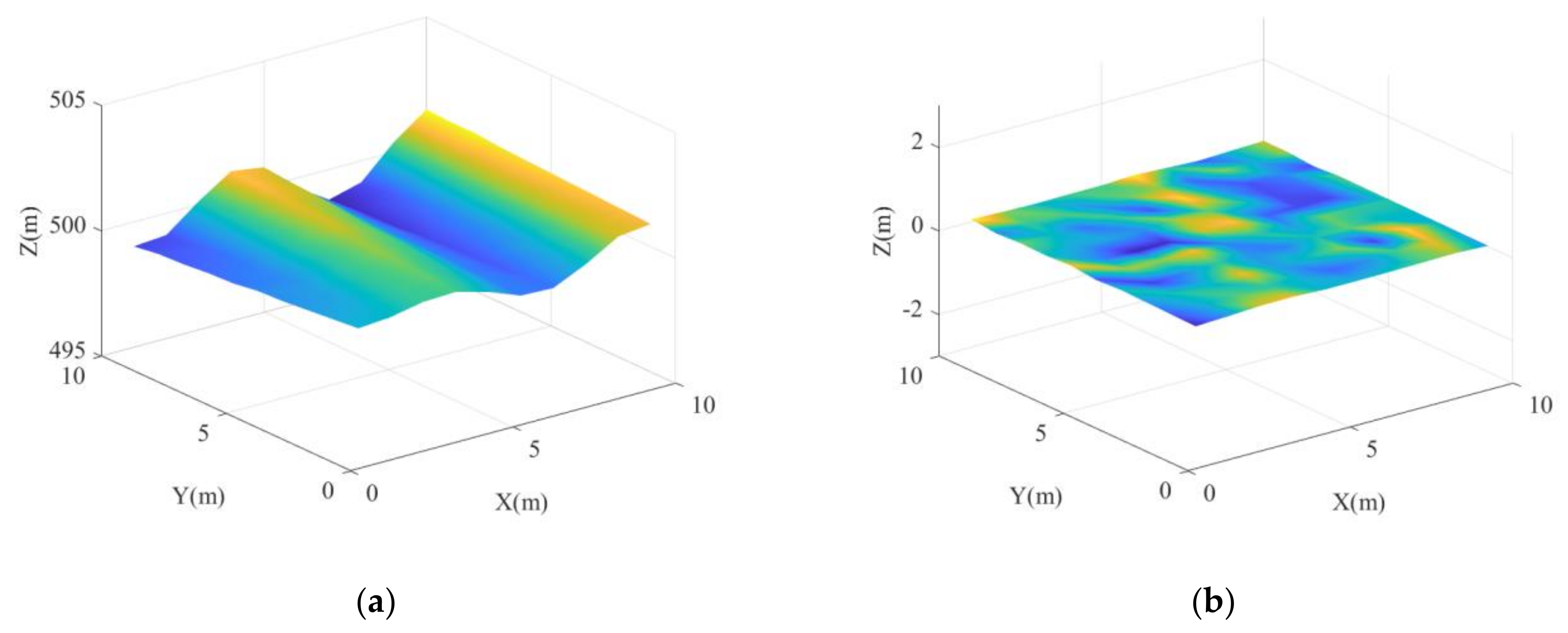
Ideal 3D imaging result (a) and 3D imaging result with time-varying vibration errors (b).
Figure 14.
Ideal 3D imaging result (a) and 3D imaging result with time-varying vibration errors (b).

Figure 15.
(a) Reconstructed 3D imaging result by using the proposed method; (b) The difference between the reconstructed and the ideal 3D imaging results.
Figure 15.
(a) Reconstructed 3D imaging result by using the proposed method; (b) The difference between the reconstructed and the ideal 3D imaging results.

Figure 16.
(a) Reconstructed 3D imaging result by using the Doppler frequency shift method; (b) The difference between the reconstructed and the ideal 3D imaging results.
Figure 16.
(a) Reconstructed 3D imaging result by using the Doppler frequency shift method; (b) The difference between the reconstructed and the ideal 3D imaging results.


Table 1.
Process flow of the proposed vibration compensation method.
| (1) | Input: The up dechirp signal and down dechirp signal . |
| (2) | Output: The estimated range of the target. |
| (3) | for |
|
(a) Separate into segmented dechirp signals and . (b) Calculate the interference signal by interfering and using Equation (15). (c) Apply Fourier transform to , and calculate the interference frequency . (d) Estimate the quadratic coefficient and establish a quadratic compensation filter using Equations (17) and (18). (e) Compensate for the quadratic vibration errors and obtain the dechirp signal by using Equation (19). (f) Apply Fourier transform to , and calculate the dechirp frequency by using Equation (20). (g) Estimate the initial velocity and establish a primary vibration compensation filter by using Equation (23). (h) Compensate for the primary vibration errors and obtain the dechirp signal by using Equation (24). | |
| end | |
| (4) | Apply Fourier transform to the up dechirp signal , and estimate the actual range by using Equation (7). |
| (5) | return. |
Table 2.
Parameters of FMCW LiDAR system.
| Parameters | Values |
|---|---|
| Waveform of LiDAR | Triangular FMCW |
| Period of the transmitted signal | 1 ms |
| Laser wavelength | 1.55 μm |
| Bandwidth of transmitted signal | 1 GHz |
Publisher’s Note: MDPI stays neutral with regard to jurisdictional claims in published maps and institutional affiliations. |
© 2021 by the authors. Licensee MDPI, Basel, Switzerland. This article is an open access article distributed under the terms and conditions of the Creative Commons Attribution (CC BY) license (https://creativecommons.org/licenses/by/4.0/).
Share and Cite
MDPI and ACS Style
Wang, R.; Wang, B.; Wang, Y.; Li, W.; Wang, Z.; Xiang, M. Time-Varying Vibration Compensation Based on Segmented Interference for Triangular FMCW LiDAR Signals. Remote Sens. 2021, 13, 3803. https://doi.org/10.3390/rs13193803
AMA Style
Wang R, Wang B, Wang Y, Li W, Wang Z, Xiang M. Time-Varying Vibration Compensation Based on Segmented Interference for Triangular FMCW LiDAR Signals. Remote Sensing. 2021; 13(19):3803. https://doi.org/10.3390/rs13193803
Chicago/Turabian StyleWang, Rongrong, Bingnan Wang, Yachao Wang, Wei Li, Zhongbin Wang, and Maosheng Xiang. 2021. "Time-Varying Vibration Compensation Based on Segmented Interference for Triangular FMCW LiDAR Signals" Remote Sensing 13, no. 19: 3803. https://doi.org/10.3390/rs13193803
Note that from the first issue of 2016, this journal uses article numbers instead of page numbers. See further details here.