
Exploiting High Geopositioning Accuracy of SAR Data to Obtain Accurate Geometric Orientation of Optical Satellite Images


1
Institute of Photogrammetry and Remote Sensing, Chinese Academy of Surveying and Mapping (CASM), Beijing 100036, China
2
Department of Built Environment, University of New South Wales (UNSW), Sydney 2052, Australia
*
Author to whom correspondence should be addressed.
Remote Sens. 2021, 13(17), 3535; https://doi.org/10.3390/rs13173535
Submission received: 4 August 2021
/
Revised: 31 August 2021
/
Accepted: 3 September 2021
/
Published: 6 September 2021
(This article belongs to the Section Earth Observation Data)
Abstract
:Accurate geopositioning of optical satellite imagery is a fundamental step for many photogrammetric applications. Considering the imaging principle and data processing manner, SAR satellites can achieve high geopositioning accuracy. Therefore, SAR data can be a reliable source for providing control information in the orientation of optical satellite images. This paper proposes a practical solution for an accurate orientation of optical satellite images using SAR reference images to take advantage of the merits of SAR data. Firstly, we propose an accurate and robust multimodal image matching method to match the SAR and optical satellite images. This approach includes the development of a new structural-based multimodal applicable feature descriptor that employs angle-weighted oriented gradients (AWOGs) and the utilization of a three-dimensional phase correlation similarity measure. Secondly, we put forward a general optical satellite imagery orientation framework based on multiple SAR reference images, which uses the matches of the SAR and optical satellite images as virtual control points. A large number of experiments not only demonstrate the superiority of the proposed matching method compared to the state-of-the-art methods but also prove the effectiveness of the proposed orientation framework. In particular, the matching performance is improved by about 17% compared with the latest multimodal image matching method, namely, CFOG, and the geopositioning accuracy of optical satellite images is improved, from more than 200 to around 8 m.
1. Introduction
Benefiting from the fast development of space transportation technology and sensor manufacturing technology, the acquisition capacity of remote sensing data has been largely enhanced [1]. Currently, it has formed a complete air–space–ground remote sensing data acquisition system which has the characteristics of being efficient and diverse (multi-platform, multisensor, multiscale) and having a high resolution (spectrum, spatial, time), providing massive unstructured remote sensing data [2]. Different types of sensors have different imaging principles and properties; therefore, different sensor data usually reflect different aspects of the ground objects and are good in different application areas. For example, optical imagery is widely applied in surveying and mapping disaster management [3], and in change detection [4]; SAR imagery is used for surface subsidence monitoring [5], DEM/DSM generation [6], and target recognition [7]; and infrared imagery is applied in soil moisture inversion [8] and forest fire monitoring [9]. Although the current processing and application technology for a single type of sensor data has reached a high level, a single type of sensor only encodes the electromagnetic wave information of a specific band. Considering the complementarity between different types of sensor data, researchers have started to fuse multi-type sensor data to solve traditional remote sensing problems, such as land cover analysis [10,11,12,13], change detection [14,15,16], image classification [17], and image fusion [18,19]. As a critical problem in the field of photogrammetry and remote sensing, topographic mapping is mainly completed using optical satellite images [20]. However, the classical orientation methods of satellite images are inefficient and have significant limitations in steep terrains. Comprehensive utilization of multi-type sensor data can be a promising solution to achieve a rapid and high-precision geometric orientation of satellite images, promoting fast and accurate global surveying and mapping [21].
The rigorous sensor model (RSM) and the rational function model (RFM) are two commonly used models to build the geometrical relationship between image coordinates and object coordinates [22]. The rational polynomial coefficients (RPCs) utilized in the RFM are derived from the RSM, and therefore the geolocation accuracy of the RFM is less than or equal to that of the RSM [23]. However, the RFM has the advantage of good universal utilization compared with the RSM, making it be simply applied to different optical satellites. Due to the inaccurate measurements of satellite location and orientation in space, high-precision geolocation is hard to achieve directly. Since the accuracy of satellite location, which is usually measured by a global navigation satellite system (GNSS), is significantly higher than that of the measured attitude angle, the measurement errors of attitude angles are the main reason for the low geolocation accuracy of optical satellite data [24]. In general, on-orbit geometric calibration [25] and external control correction [26] are two typical methods to improve the geo-localization accuracy. In particular, the external control information can be provided by traditional field-measured ground control points (GCPs) [27,28,29], topographic maps, or orthoimage maps [30,31]. Measuring GCPs in the field costs a high amount of manual work and is not applicable in dangerous areas, while the method of using reference images [32] is simpler and more efficient, where the GCPs are obtained from manual selection or automatic image matching. However, reference images are not available in most cases, restricting their wide application.
As active remote sensing satellites, the imaging principle and data acquisition concept of SAR satellites are significantly different from those of optical satellites. In particular, SAR satellites measure the backscattered signals from the reflecting ground objects in a side-view mode (angle between 20 and 60 with respect to the nadir direction) along the flight path. In the post-processing process, pulse compression technology is used to improve the range resolution, and synthetic-aperture technology is used to simulate the equivalent large-aperture antenna to improve the azimuth resolution so that the SAR satellite image always has a high spatial resolution [33]. For example, the spatial resolution of TerraSAR-X is 1.5 × 1.5 m in spotlight mode, and 3 × 3 m in stripmap mode [34]; the spatial resolution of GF-3 is 1 × 1 m in spotlight mode, and 3 × 3 m in stripmap mode [35]; and the spatial resolution of TH-2 is 3 × 3 m in stripmap mode [36]. Benefiting from the approximate spherical wave emitted by the radar antenna and the measurement scheme of SAR satellites, the geo-localization accuracy is not sensitive to the satellite attitude and weather conditions. In addition, SAR satellite images exhibit high geopositioning accuracy due to the precise orbit determination technology and atmospheric correction model. Bresnahan [37] evaluated the absolute geopositioning accuracy of TerraSAR-X by using 13 field test sites and found that the RMSE value is around 1 m in spotlight mode and 2 m in stripmap mode. Eineder et al. [38] verified that the geometric positioning accuracy of TerraSAR-X images can reach within one pixel in both the range and azimuth directions and even reach centimeter level for specific ground targets. Lou et al. [36] investigated the absolute geopositioning accuracy of a Chinese SAR satellite, TH-2, in a few calibration fields distributed in China and Australia and found that the RMSE value reaches 10 m.
Considering the high and stable absolute geopositioning accuracy, SAR satellite data can be a reliable source for proving high-precision control information for an accurate orientation of optical satellite images, which can be obtained in most areas worldwide. Similar to the methods using orthoimage maps, tie points are identified between the SAR orthophoto and the optical satellite image, and these tie points are taken as GCPs to improve the orientation accuracy of optical satellite images [39,40]. Reinartz et al. [41] used adaptive mutual information to match the SAR and optical satellite images, and the matches were employed to optimize the original RPCs. The results showed that the geometric positioning accuracy of the optical satellite is largely improved and reaches within 10 m. However, this method does not consider the complex terrain and cannot work with multiple SAR reference images. Merkle et al. [42] used a large number of pre-registered TerraSAR-X and PRISM image datasets to train a Siamese neural network and used the network model to extract the corresponding points between the SAR and optical satellite images. The matching points were employed to optimize the sensor model, enhancing the geo-localization accuracy. However, this method cannot handle optical satellite and SAR images with large offsets and cannot work on large optical satellite images due to the limited GPU memory.
The significant difference in acquisition principles, viewing perspectives, and wavelength responses between SAR and optical satellite images makes finding reliable correspondences when matching optical and SAR images challenging [42]. More specifically, SAR sensors acquire data in a sideways-looking manner, which may cause typical geometric distortions such as foreshortening, occlusion, and shadowing, especially for the areas with large height changes. In contrast, optical satellite images are acquired in the nadir view or small fixed slanted angles to provide high geometric accuracy. Consequently, the same object may have a completely different appearance on SAR and optical satellite images. Moreover, these two types of sensors receive and apply electromagnetic waves in different bands. The radar signal wavelength is at the level of centimeters, while that of optical signals is in nanometers. The different lengths of waves encode different aspects of object properties, therefore leading to significant intensity differences between SAR and optical satellite images for the same object. Additionally, the signal polarization, roughness, and reflectance properties of the object surface may also influence the wavelength responses greatly. In addition, the speckle effect on SAR images further increases the matching difficulty of optical satellite images. Figure 1 shows the difference between an optical and a high-resolution SAR image for a selected scene containing manufactured structures and vegetation.
In this paper, we propose an improved multimodal image matching descriptor angle-weighted oriented gradient (AWOG) for SAR and optical satellite images, obtaining a robust and accurate matching performance. To describe the image features, we calculated a multi-dimensional feature vector lying on multiple uniform distribution orientations based on the horizontal and vertical gradient maps and for each pixel, as with the recent multimodal image matching method CFOG [43]. Note that the range of [0°, 180°) was divided into several evenly distributed orientations, and we calculated the gradient direction and magnitude based on and , found the two orientations nearest to the image gradient direction, and distributed the gradient magnitude to these two orientations based on their weights. In this way, the image gradient value is only allocated to the two most related orientations rather than all orientations, increasing the distinguishability of feature vectors. During the process, we opened a window image on the whole image and assigned the two weighted amplitudes of each pixel in the window image to the corresponding orientation elements of the feature vector. After all the gradients of pixels in the window image were assigned, the feature vector of the target pixel was obtained and normalized to reduce the influence of the nonlinear intensity difference. In addition, we introduced a quick lookup table named the feature orientation index (FOI), which converts the inefficient calculation of each pixel into matrix operations and helps to assign the weighted values to their corresponding elements of the feature vector, significantly improving the computation efficiency. Additionally, in terms of metric similarity, we utilized phase correlation (PC) [44] rather than the metrics in the spatial domain to speed up the matching process, but we omitted the normalization operation of PC since the descriptor was normalized during the feature vector generation.
In addition, we propose a precise geometric orientation framework for raw optical satellite images based on SAR orthophotos. Specially, we first collected all available SAR images of the study area and performed overlap detection between the SAR images and the target optical satellite image. Only the SAR images with large overlaps were retained as the reference image sets. Then, we created image pyramids for the optical satellite images and all the reference SAR images and detected feature points using the SAR-Harris feature detector [45]. To ensure the uniformity and high discrimination of the obtained feature points simultaneously, we introduced an image block strategy. After that, we transferred the point features into their corresponding ground points and reprojected the ground points onto the optical satellite images. The reprojected locations on the satellite image were taken as the initial correspondences for the feature points of SAR images, which were optimized using AWOG. We further conducted error elimination to remove the unreliable matches. We deemed the retained matches to be correct and took them as virtual control points (VCPs). Finally, we took the VCPs and the optical satellite image as input and performed RFM-based block adjustment to achieve an accurate image orientation of the optical satellite images.
In summary, the main contributions of our work are as follows:
- We propose a robust feature descriptor AWOG to match SAR and optical satellite images and introduce a PC-based matching strategy, obtaining stable and reliable matching point pairs with higher efficiency.
- We put forward a framework for an accurate geometric orientation of optical images using the VCPs provided by SAR images.
- Various experiments on SAR and optical satellite image datasets verify the superiority of AWOG to the other state-of-the-art multimodal image matching descriptors. Compared with CFOG, the correct matching ratio is improved by about 17%, and the RMSE of location errors is reduced by about 0.1 pixels. Additionally, the efficiency of the proposed method is comparable to CFOG and about 80% faster than the other state-of-the-art methods such as HOPC, DLSS, and MI.
- We further prove the effectiveness of the proposed method for the geometric orientation of optical satellite images using multiple SAR and optical satellite image pairs. Significantly, the geopositioning accuracy of optical satellite images is improved, from more than 200 to around 8 m.
This paper is structured as follows: Section 2 introduces some related works on SAR and optical image matching. Section 3 presents the proposed matching method for SAR and optical satellite images. Section 4 introduces a general orientation framework of optical satellite images using SAR images. Section 5 presents the experiments and analysis concerning the proposed method. Section 6 discusses several vital details. Finally, we conclude our work and discuss future research directions in Section 7.
2. Related Work
Current SAR and optical satellite image matching studies can be roughly divided into feature-based and area-based methods [46].
Feature-based methods detect salient features on images and match them based on similarity. The features can be seen as a simple representation of the whole image, thus being robust to geometric and radiometric changes, and can be classified into corner features [47,48], line features [49,50], and surface features [51]. Towards matching SAR and optical satellite images, Fan et al. [52] proposed the SIFT-M algorithm by extracting SIFT [53] features on both images, constructing distinct feature descriptors from multiple support regions, and introducing a spatially consistent matching strategy to match these feature points. Compared to SIFT, SIFT-M obtains more matches and has higher efficiency and accuracy. Based on SIFT-M, Xiang et al. [54] further proposed the OS-SIFT algorithm. They detected feature points in a Harris-scale space built on the consistent gradients of both SAR and optical satellite images and computed the histograms of multiple image patches to enhance the distinguishability of feature descriptors, increasing the robustness and performance of SIFT-M. Salehpour et al. [55] proposed a hierarchical method based on the BRISK operator [56]. They used an adaptive and elliptical bilateral filter to remove the speckle noise on SAR images and introduced a hierarchical approach to utilize the local and global geometrical relationship of BRISK features. This method has high accuracy, but the obtained matches are few and not well distributed over the full image. To improve the robustness against the significant nonlinear radiation distortions of SAR and optical images, Li et al. [57] proposed a radiation-variation insensitive feature transform (RIFT) method. This approach first detects feature points on the phase congruency map [58], which considers the repeatability and number, and then constructs a maximum index map (MIM) based on the log-Gabor convolution sequence. Moreover, they achieved rotation invariance by analyzing the value changes of the MIM. The results showed that RIFT performs well and is stable on multimodal image matching. Based on RIFT, Cui et al. [59] further proposed SRIFT. They first established a multiscale space by using a nonlinear diffusion technique. Then, a local orientation and scale phase congruency (LOSPC) algorithm was used to obtain sufficiently stable key points. Finally, a rotation-invariant coordinate (RIC) system was employed to achieve rotation invariance. Compared to RIFT, SRIFT obtains more matches and strengthens the robustness against scale change. Wang et al. [60] proposed a phase congruency-based method to register optical and SAR images. This method consists of employing a uniform Harris feature detection method and a novel local feature descriptor based on the histogram of the phase congruency orientation. The results showed that the ROS-PC is robust to nonlinear radiometric differences between optical and SAR images and can tolerate some rotation and scale changes. To increase the discriminability of the classical local self-similarity (LSS) descriptor [61], Sedaghat et al. [62] proposed a distinctive order-based self-similarity descriptor (DOBSS) based on the separable sequence. To fulfill multimodal image matching, they first extracted UR-SIFT [63] feature points from both images, constructed DOBSS descriptors, and finally utilized cross-matching and consistency checks in the projective transformation model to find the correct correspondences. This method not only obtains more matches but also shows better robustness and accuracy than SIFT and LSS. Beyond the methods based on point features, Sui et al. [64] proposed a multimodal image matching method by combing iterative line feature extraction and Voronoi integrated spectral point matching, increasing the matching reliability. However, this method requires a large number of lines in the scene. Hnatushenko et al. [65] proposed a variational approach based on contour features for co-registration of SAR and optical images in agricultural areas. They performed a special pre-processing of SAR and optical images and achieved co-registration by transforming it into a constrained optimization problem. This method is quite efficient and fully automatic. Xu et al. [66] proposed a surface feature-based method that employs iterative level set-based area feature segmentation to take advantage of the surface features. However, this method can only be applied to images containing significant regional boundaries, such as lakes and farmland. Even though the features have the advantage of flexibility and robustness on multimodal images, the repeatability is relatively low due to the large geometric deformations, and nonlinear intensity changes [67,68]. For example, the state-of-the-art method RIFT only has an inlier ratio of about 15%, decreasing the performance of feature-based methods in matching SAR and optical satellite images.
The area-based methods realize image matching by opening a matching window on the original images and utilizing a similarity metric to find the matches [69]. Normalized cross-correlation (NCC) [70] and mutual information (MI) [71] are two popularly used metrics in the matching of optical satellite image pairs. However, NCC cannot handle the matching of SAR and optical images in most cases due to the nonlinear intensity deformation. On the contrary, MI describes statistical information of the image and has good robustness to nonlinear change. However, the MI method does not consider the influence of neighborhood pixels, making it easily fall into the local extremum. Moreover, MI is sensitive to the image window size and requires a large amount of calculation. Suri and Reinartz [72] analyzed the performance of MI on the registration of TerraSAR-X and Ikonos imagery over urban areas and found that the MI-based method can successfully eliminate large global shifts. Apart from MI, which works on multimodal image matching, another method is to reduce the multimodal images into a uniform form. The phase correlation (PC) algorithm developed by Kuglin and Hines [44] can be used to transform both SAR and optical satellite images into the frequency domain. This approach shows some robustness against nonlinear intensity distortion and has high efficiency. To explore the inherent structure information of SAR and optical satellite images, Xiang et al. proposed the OS-PC algorithm [73] by combining robust feature representations and three-dimensional PC, which exhibits high robustness to radiometric and geometric differences.
Some researchers noticed that even though large nonlinear intensity differences exist between SAR and optical satellite images, the morphological region features remain [74,75]. Therefore, these researchers first extracted the image conjugated structure and then conducted matching of the structural image, increasing the matching performance. Li et al. [76] used the histogram of oriented gradients (HOG) descriptor [77] to express the image structure and used NCC as the measured metric, obtaining good matching results. Based on HOG, Ye et al. [78] proposed the histogram of oriented phase congruency (HOPC) feature descriptor by replacing the gradient feature with a phase congruency feature, obtaining good performance on the matching of SAR and optical satellite images. Zhang et al. [79] applied HOPC to a combined block adjustment framework for optical satellite stereo imagery which is assisted by spaceborne SAR images and laser altimetry data. Ye et al. [80] further proposed a similarity metric, DLSC, using the NCC of a novel dense local self-similarity (DLSS) descriptor which is based on shape properties. Since DLSS captures the self-similarities within images, it is robust to large nonlinear intensity distortions. However, HOG, HOPC, and DLSS only construct descriptors for a few silent features. Thus, they are both sparse representations and omit some available and important structure information. Aiming at solving this issue, Ye et al. [43] further proposed the channel features of oriented gradients (CFOG). CFOG computes the adjacent structure feature pixel by pixel, enhancing the ability to describe the structure details. In terms of the similarity metric, they applied the convolution theorem and Fourier transform to deduce the sum of squared differences (SSD) measure from the spatial domain to the frequency domain, achieving a fast calculation. Ye et al. [81] used CFOG to fulfill the co-registration of Sentinel-1 SAR and Sentinel-2 optical images and evaluated the performance of various geometric transformation models, including polynomials, projective models, and RFMs. However, CFOG only computes the gradient maps in the horizontal and vertical directions and uses them to interpolate the gradients in all the other orientations, which brings ambiguity and decreases the accuracy.
With the development in the field of deep learning, some researchers have explored the application of deep learning-based techniques to fulfill the matching of SAR and optical satellite images. Merkle et al. [82] investigated the possibility of cGANs (conditional generative adversarial networks) in this task. They first trained conditional generative adversarial networks to generate SAR-like image patches from optical satellite images and then achieved the matching of SAR and optical images using NCC, SIFT, and BRISK under the same image model. Following the same thought, Zhang et al. [83] employed a deep learning-based image transfer method to eliminate the difference between SAR and optical images and applied a traditional method to match the multimodal remote sensing images. Ma et al. [84] proposed a two-step registration method to register homologous and multimodal remote sensing images. They first computed the approximate relationship with a deep convolutional neural network, VGG-16 [85], and then adopted a robust local feature-based matching strategy to refine the initial results. Similarly, Li et al. [86] applied a two-step process to estimate the rigid body rotation between SAR and optical images. They first utilized a deep learning neural network called RotNET to coarsely predict the rotation matrix between the two images. After that, a better matching result was obtained using a novel local feature descriptor developed from the Gaussian pyramid. Zhang et al. [87] set up a Siamese fully convolutional network and trained it with a loss function that maximizes the feature distance between the positive and negative samples. Mainly, they built a universal pipeline for multimodal remote sensing image registration. Hughes et al. [88] developed a threefold approach for the matching of SAR–optical images. They first found the most suitable matching regions using a goodness network, then built a correspondence heatmap with a correspondence network, and finally eliminated the outliers by an outlier reduction network. Even though these methods obtained better results than the competing traditional geometric-based methods in their experimental results, current deep learning-based methods still suffer from the following problems. Firstly, there is no multimodal remote sensing dataset large enough to train a deep learning neural network for general use. Secondly, the deep learning-based methods bring challenges to the computer resources, especially the GPU, and the efficiency is relatively low under most computer setups. Finally, the current learning-based methods cannot be applied to full-scale satellite remote sensing images. These demerits restrict the practical application of deep learning techniques in the matching or registering of multimodal remote sensing images.
3. Accurate and Robust Matching of SAR Images and Optical Satellite Images
3.1. AWOG Descriptor
Since the gradient information can describe the image structure well and is robust to nonlinear intensity differences, we also constructed our multimodal image descriptor AWOG based on image gradients as with the other state-of-the-art image descriptors. However, unlike those descriptors that build sparse feature descriptors only for silent features such as HOPC [78] and DLSS [80], AWOG constructs dense descriptors for each pixel, increasing the description ability of image details. Even though CFOG [43] is also based on dense descriptors, it uses the horizontal and vertical gradients to interpolate the gradients in multiple other directions, which decreases the distinctiveness of the features. On the contrary, AWOG uses an angle weighting strategy to distribute the gradient value only into the two most related orientations, largely increasing the distinguishability of the feature descriptors and further improving the matching reliability of SAR and optical satellite images.
AWOG first calculates the image gradients as the basis for the subsequent calculation. As displayed in Figure 2, the horizontal gradient and vertical gradient are firstly calculated using the Sobel operator [89], and then the gradient magnitude and gradient direction of the image are calculated based on equations (1) and (2). Since there may be an intensity inversion between SAR and optical satellite images, we conducted gradient direction modification [43,90,91,92] to improve the resistance against such intensity appearance. Significantly, the gradient direction whose values are greater than 180 is subtracted by 180, as in Equation (3).
where and are the gradient magnitude and direction, respectively.
In order to make full use of the gradient information, we first divided the range of into subranges evenly by a few discrete and continuous orientation values (as shown in Figure 3); the number of values was the same as the size of the feature vector; and the index numbers of these values corresponded to those of the feature orientations used for building the feature vector. Then, we introduced a feature orientation index table () to speed up the following calculation process. For a single pixel, its gradient direction value must lie in a certain subrange, and we named the indexes of the lower and upper bounds of the subrange for a pixel as and , respectively. Note that is always one greater than . The table can be obtained from collecting the of all pixels, which can be calculated from Equation (4).
where the symbol means to take an integer not greater than the value in it.
Note that the feature vector was initialized as , and we utilized the angle difference of the gradient direction with the two feature orientations corresponding to the orientation indexes and of each pixel as weights and assigned the gradient magnitude onto the two feature orientations based on the calculated weights. The smaller the angle difference between the gradient direction and a predefined feature orientation, the larger the gradient magnitude value assigned to that feature orientation.
Furthermore, we utilized adjacent information to reduce the influence of nonlinear intensity distortions between SAR and optical satellite images. To improve the calculation efficiency, we introduced two weighted gradient magnitude images, and , which can be obtained by collecting the weighed values of the gradient magnitude distributed to the lower and upper feature orientations corresponding to and of each pixel, respectively. The calculation can be expressed as the following equation:
where and are the weighted values, and and are the weighted gradient magnitude images.
During processing, we took the target pixel as the center to simultaneously open up statistical windows of pixels on and and assign the values of each pixel in the windows to the corresponding elements of the feature vector with the . The statistical process is similar to voting, where all the feature vector elements are used as ballot boxes, and the values of and are used as the vote value. The statistical process is shown in Figure 4. For a specific element of the feature vector of the target pixel, it can be seen as the sum of two parts. The first part is the sum of all pixel values with equal to in the statistical window, and the second part is the sum of all pixel values with equal to in the statistical window, which can be expressed by Equation (6). The feature descriptor is obtained after finishing the calculation for all predefined feature orientations of the feature vector. If we arrange the feature vector at each pixel along the z-axis direction perpendicular to the image plane, a 3D image cube can be formed, which is easy to be displayed.
where means a specific element of the feature vector, and and are calculated by statistical processing.
To reduce the influence of orientation distortions caused by local deformations, we conducted convolution on the feature 3D cube with a kernel of in the direction [43]. After that, we further normalized the feature vector using the norm with Equation (7).
In summary, the whole pipeline of AWOG is shown in Figure 5.
3.2. Phase Correlation Matching
Traditional similarity measures in the spatial domain such as NCC are very time-consuming for high-dimensional feature vectors. Thus, we utilized the 3D phase correlation (PC) [73] based on the frequency to match the image features, improving the calculation efficiency. Since AWOG conducts normalization during construction, we no longer need to normalize the cross-power spectrum as the traditional PC does.
The core idea of PC is the Fourier shift property which converts the offset of image coordinates into a linear phase difference in the frequency domain [93]. Generally, PC first transfers the image into the frequency domain by the Fourier transform and calculates the cross-power spectrum. If and are the AWOG descriptors of the reference image and the input image, respectively, then
Given that and are obtained by conducting 3D fast Fourier transform of and , Equation (9) can be calculated according to the Fourier shift theorem.
where is the 3D unit vector.
By conducting some deformations, the cross-power spectrum can be calculated as follows:
where * indicates the complex conjugate.
Through analyzing the inverse Fourier transform of the cross-power spectrum , a correlation function centered at can be obtained. Additionally, the peak value of the function always appears at ; thus, the corresponding point can be found by locating the maximum value, which can be expressed as follows:
where denotes the inverse transform of the 3D fast Fourier transform, and denotes the correlation function, which is centered at .
In order to testify the performance of PC, we conducted experiments on a pair of high-resolution optical satellite and SAR images that cover the same urban area and have a large nonlinear intensity difference and compared our results with those of NCC. As shown in Figure 6, we can see that the results of PC and NCC with the AWOG descriptor both only have one single peak, which means they all find the correct matches. However, the running time for PC is 0.01 s, while that of NCC is 3.2 s. Therefore, the use of PC as a similarity measure not only keeps the high accuracy of NCC but also largely improves the efficiency.
4. A General Orientation Framework of Optical Satellite Images Using SAR Images
In this section, we put forward a general framework for the automatic orientation of optical satellite images based on SAR orthophotos. Firstly, we perform overlap detection between the optical satellite image and SAR images to find the qualified images as the reference SAR image set. Then, the image pyramids are constructed for all the SAR and optical satellite images. The SAR-Harris feature point detector, combined with an image dividing strategy [94], is utilized on the pyramid images to retain enough high-quality features across the entire image. After that, the SAR image and DEM data are used for rough geometric correction to coarsely eliminate the rotation and scale differences, and AWOG is applied on the rectified images to obtain accurate corresponding points, which are taken as virtual control points (VCPs). Finally, RFM-based block adjustment [95] is carried out for the optical satellite image by using the VCPs, and the accurate orientation parameters are output. The specific steps are as follows:
(1) The available SAR images of the target study area are collected, and the helpful reference SAR image set is built through overlap detection. We check the corresponding ground cover of SAR images and the optical satellite image, and only the SAR images with overlapping ground areas are retained as reference images. Specially, we read the metadata of the SAR reference image to obtain the coordinates of the four image corners and other affiliated information and project the four corners onto the ground. In this way, the longitude and latitude ranges of the ground covering of the SAR reference image are obtained. For the optical satellite image, we can directly obtain the coordinates of the ground covering by reading the metadata of the optical satellite image. If there are overlaps between the two ground coverings, we deem these two images overlapped; otherwise, there is no overlap between these two images.
(2) Image pyramids are constructed for the optical satellite and reference SAR images, and high-quality feature points are detected on the SAR images. If the resolution difference between the reference image and the optical satellite image is not more than double, the image pyramid layer and the zoom ratio between different levels are set as 4 and 2, respectively. Suppose the resolution difference between the images is large. In that case, a certain number of pyramid image layers are added to the higher-resolution image according to the multiple of the resolution difference, and a lookup table is established to match the images between the levels with a smaller resolution difference. Then, the SAR-Harris corner detector [45] is employed to detect feature points on each layer of the pyramid image of the reference SAR image. Additionally, a block strategy [94] is also applied to ensure the uniformity of the point distribution. All the subsequent steps start with the top layer pyramid image.
(3) There are always large geometric deformations between the optical satellite and SAR images. Therefore, we first perform image reshaping (as shown in Figure 7) to coarsely eliminate the rotation and scale difference and then use AWOG to match the images. First, the template window is determined on the reference SAR image with the obtained feature point as the center, and the ground area corresponding to the template window is acquired based on the approximate DEM of the study area, which can be provided by SRTM. To obtain the rough matching area, we reproject the ground area onto the optical satellite image with the RFM. Furthermore, an affine transformation model between the searching area of the optical satellite image and the template window of the reference image is established. The searching area of the optical satellite image is resampled using the bilinear interpolation method according to the established transformation model in order to eliminate the rotation and scale difference. At last, AWOG is applied to match the roughly geo-rectified image with the reference SAR image, and the RANSAC algorithm is utilized to eliminate unreliable matches.
(4) The RFM-based affine transformation compensation model [95] is performed to improve the orientation accuracy of the original RPCs, and this process is completed using block adjustment with multiple reference SAR images. The affine transformation model has been widely applied to compensate the deviation of RPCs for high-resolution optical satellite images, which can be expressed as follows:
where and are the column and row of tie points in the optical satellite image, and and () are the unknown affine model parameters. In particular, and compensate the row direction and column direction errors on the image caused by the attitude and position inaccuracy in the satellite moving and scanning directions of the CCD linear sensor, respectively; and compensate the error caused by the drifts of the inertial navigation systems and GPS, respectively; and and compensate the error caused by an inaccurate image interior orientation.
In order to obtain the corresponding initial positions of the image points in the SAR reference image on the optical satellite image, we first need to obtain the geographic coordinates of the image point in the SAR reference image, which can be calculated as follows:
where and are the longitude and latitude of point with image coordinates and (index s denotes the SAR scene). and are the projection coordinates of point . is a transformation function to transform point coordinates from the projection system to the reference system. and are the projection coordinates of the upper left corner of the SAR reference image, and and are the resolution of the SAR reference image in the column direction and row direction, respectively.
After obtaining the corresponding ground points of the feature points in the reference image, the back-projection location of these ground points on the optical satellite image can be calculated using the RPCs and DEM of the target area, which are provided by the SRTM in this study.
where and are the normalized image coordinates of the tie point computed by the forward rational functions of the optical satellite image. are the normalized longitude, latitude, and altitude of the tie point .
For each tie point on the optical image, through combing Equations (12) and (14), the block adjustment can be described as
where and denote the column and row of the tie point in the optical image, which is acquired by performing image matching, and and are the un-normalized image coordinates of the tie point after back-projection using the RPCs.
Finally, the optimal estimations of affine transformation parameters and are obtained by iterative least squares adjustment.
(5) The processing status is checked frequently. If the bottom layer of the pyramid image has completed the calculation, the final affine correction transformation model together with the original RPCs is output as the accurate orientation result. Otherwise, we transmit the calculation results of the current layer of the pyramid to the next layer until the bottom layer. The flowchart of this orientation framework is shown in Figure 8.
5. Experiments and Analysis
In this section, we first verify the superiority of our proposed image matching method over state-of-the-art multimodal image matching methods and then prove the effectiveness and robustness of the proposed orientation framework of satellite optical images using SAR reference images.
5.1. Matching Performance Investigation
5.1.1. Experimental Datasets
To testify the performance of AWOG, six optical-to-SAR image pairs covering the same scene were unitized. Considering the significant image property difference between LiDAR and optical images, we also used two LiDAR-to-optical image pairs to verify the robustness of our method. These image pairs were acquired at different imaging times and cover rich image contents. Figure 9 presents all the experimental image pairs. All the image pairs were pre-rectified to the same spatial resolution, and there are no large scale, rotation, and translation differences. However, there are still large geometric deformation and noticeable nonlinear intensity changes between the image pairs. The detailed information of the experimental images is shown in Table 1.
5.1.2. Evaluation Criteria
Three commonly used criteria were employed to indicate the matching performance, which are the correct matching ratio (CMR), root mean square error (RMSE), and average running time (t). The correct matching ratio describes the matching success rate, which can be calculated by dividing the number of correct matches by all obtained matches. To determine the correct matches, we first manually selected 50 obvious points from both images as checkpoints and calculated the transformation between images. Then, the matches whose location errors are smaller than 1.5 pixels were deemed correct matches. RMSE represents the matching accuracy of correct matches. The smaller the value of RMSE, the higher the accuracy. is the average running time on all experimental image pairs, which reflects the matching efficiency.
5.1.3. Comparison with the State-of-the-Art Multimodal Image Matching Methods
To verify the effectiveness and superiority of the proposed method, we compared our method with three state-of-the-art methods, namely, DLSS [80], HOPC [78], and CFOG [43]. In addition, MI [71] was also utilized as a baseline considering its good robustness against nonlinear intensity changes. AWOG and CFOG calculate the descriptor pixel by pixel; therefore, they can be matched by using PC or SSD. Meanwhile, HOPC and DLSS only calculate the descriptor in a sparse sampled grid, meaning they can only be matched with the similarity measures in the spatial domain such as SSD; PC does not work on them. To evaluate the descriptors comprehensively and fairly, we matched AWOG and CFOG with PC and used SSD as the similarity measure for all four descriptors. For convenience, we named the combinations of AWOG and PC, CFOG and PC, AWOG and SSD, CFOG and SSD, HOPC and SSD, and DLSS and SSD as AWOGPC, CFOGPC, AWOGSSD, CFOGSSD, HOPCSSD, and DLSSSSD, respectively.
Before matching, 200 SAR-Harris feature points were firstly detected on the reference image, and then the points were described and matched with different approaches. For MI, DLSSSSD, HOPCSSD, CFOGSSD, and AWOGSSD, a template window image with sizes from 25 × 25 to 91 × 91 pixels was opened on the reference image, and the correspondences were found through moving the template window in searching areas from 46 × 46 to 111 × 111 pixels. For AWOGPC and CFOGPC, they were directly matched with the template window image without sliding.
Figure 10 presents the results of all comparative methods with respect to the CMR. Overall, we can see that the proposed method AWOGPC performs the best, while MI obtains the worst results, and the reason could be that MI does not consider the adjacent information during matching, which may fall into a local optimum.
The results of DLSSSSD, HOPCSSD, CFOGSSD, and AWOGSSD provide a fair comparison of the feature descriptors employed directly and fairly, considering that they all utilize the same similarity measure, SSD. DLSSSSD is easily affected by the properties of the image content, and it performs worse on image pair 6 with mountain coverage and image pair 8 that contains a textureless LiDAR depth map. HOPCSSD and CFOGSSD both obtain a better performance than DLSSSSD, showing good resistance against nonlinear intensity changes. AWOGSSD obtains the highest CMR among all comparative methods on all datasets, proving the superiority and robustness of the proposed descriptor, AWOG.
Moreover, CFOGPC and AWOGPC perform better than CFOGSSD and AWOGSSD, respectively, which proves the effectiveness of the similarity measure PC when applied to multimodal image matching. Compared with CFOGPC, AWOGPC achieves better results than CFOGPC, benefiting from the stronger gradient description ability. In particular, AWOGPC is less sensitive to the size of the template window image. For example, the CMR of AWOGPC is 17.1% higher than that of CFOGPC on average under the template window with a size of 31 × 31 pixels.
Figure 11 presents the RMSE of all methods with a template window of 91 × 91 pixels, and the exact RMSE values are provided in Table 2. Again, MI shows the worst result. AWOGSSD obtains the smallest RMSE compared to all the other methods that also utilize SSD. CFOGPC and AWOGPC perform better than CFOGSSD and AWOGSSD, respectively. Furthermore, the RMSE of AWOGPC is smaller than CFOGPC, displaying the highest accuracy among all comparative approaches. In particular, the average value of RMSE on all datasets of AWOGPC is 0.135, 0.146, 0.192, 0.214, 0.269, and 0.414 pixels better than CFOGPC, AWOGSSD, CFPGSSD, HOPCSSD, DLSSSSD, and MI on average, respectively.
Figure 12 presents the average running time of all methods under different sizes of template window images on all datasets, and the corresponding values are presented in Table 3. For the methods using SSD, the computational efficiency of HOPCSSD and CFOGSSD is at the same level. At the same time, DLSSSSD achieves the highest calculation efficiency, and AWOGSSD has the lowest calculation efficiency due to the relatively complex computation of a complete descriptor for all pixels. Generally, the methods using PC are faster than the corresponding methods under the same window size. In detail, CFOGPC and AWOGPC are faster than CFOGSSD and AWOGSSD, respectively. Moreover, the running time of CFOGPC and AWOGPC increases much slower than that of CFOGSSD and AWOGSSD with the increase in the size of the matching image window. In detail, when the size of the template window is 25 × 25 pixels, the running times of CFOGPC, AWOGPC, CFOGSSD, and AWOGSSD are 0.510 s, 1.279 s, 1.428 s, and 3.019 s, respectively; the running times become 0.888 s, 1.652 s, 10.307 s, and 15.866 s when the size of the template window is 91 × 91 pixels. We can see that AWOGPC is slightly slower than CFOGPC, but much faster than CFOGSSD and AWOGSSD, showing great advantages in practical application.
Overall, AWOGPC shows a good balance between accuracy and efficiency, achieving the best accuracy and a relatively good efficiency among all competing methods. Therefore, AWOGPC can be well applied to the matching work of multimodal images. Figure 13 provides the visual matching results of AWOGPC on all experimental image pairs. From the result, we can see that a large number of evenly distributed matches with high accuracy are obtained, proving the effectiveness of the proposed method.
5.2. Geometric Orientation Accuracy Analysis
5.2.1. Study Area and Datasets
To evaluate the performance and effectiveness of the automatic orientation of optical satellite images using SAR reference images, several experiments were conducted on the location of Guangzhou city and its surrounding areas in China. As shown in Figure 14, the length of the study area is about 170 km from north to south, and the width of the area is about 140 km from east to west. The western and southwestern parts of the study area are relatively flat, the southern part is the estuary of the Zhujiang River, and the rest is mountainous areas where the elevation of the central mountainous area is around 200~500 m. The largest elevation difference in the northeastern mountainous area is close to 1200 m.
The TerraSAR-X orthoimages were taken as the reference images, whose spatial resolution is 5 m. Their plane positioning accuracy is better than 5 m which has been testified by field-measured checkpoints. The optical satellite images to be oriented are the panchromatic images from GF-1, GF-2, and ZY-3 satellites, which have a location difference of 99.6~260.4 m from the reference images measured manually. The amount and detailed information of the experimental images are provided in Table 4. Moreover, we used SRTM-30 to provide the elevation information for the object points.
The distribution of the reference SAR images and optical satellite images is displayed in Figure 15. We can see that the coverage of the SAR reference images mainly locates in the north-central region of the study area, and there is a specific range of vacancy in the southeast region. The four GF-1 satellite images cover all available reference images in the study area, of which a small part of the GF-1-1 and GF-1-3 images and about one third of the GF-1-2 and GF-1-4 images have no reference information. All four GF-2 images fall into the coverage of the reference images. The three ZY-3 images locate in the midwest of the coverage of the reference images, of which about one third of the ZY-3-1 images and a small part of the ZY-3-2 and ZY-3-3 images do not have reference information.
5.2.2. Geometric Orientation Performance
Before starting the orientation process, there are several parameters required to be set. Based on the analysis of AWOGPC in Section 5.1, we set the values of m, n, and the size of the template window image as 3, 8, and 61 × 61 pixels. Additionally, for the parameters used in the orientation process, we set the size of the template window image on the top layer of the image pyramid as 121 × 121 pixels, and the number of iterations and the gross error threshold of RANSAC as 2000 and 3 pixels, respectively.
Figure 16 displays the obtained matches between the optical satellite image GF-1-3 and all available reference SAR images of it. Figure 16a–g show the matching points at each SAR image, and Figure 16h shows the gathering of all corresponding matching points on GF-1-3, where the color of a point indicates the images to which it is matched. From Figure 16, we can see that the matching points are not only large in number but also evenly distributed throughout the image, enabling them to be good virtual control points (VCPs).
Table 5 presents the detailed quantitative results. From the index of NO, we can see that each optical satellite image has a large number of VCPs. There are still 9046 VCPs obtained for the GF-1-3 image, whose coverage is mainly mountains. Additionally, after orientation, the differences in the coordinates of the corresponding locations between the SAR reference images and optical satellite images are between 0.81 and 1.68 pixels, and from 4.1 to 8.4 m when transferring to the object space. Considering the high geopositioning accuracy of SAR images, the geometric orientation of the optical satellite images is significantly improved. Moreover, the proposed method has high efficiency. The processing time of the GF-2-1 images is only 33.15 s. Generally, the running time increases with the number of reference images. For example, the processing time of GF-1-1 is less than that of GF-1-4, even though more matches are found for GF-1-1 considering the reference images of GF-1-1 total six, while those of GF-1-4 total seven. In particular, the running time becomes 98.18 s when there are seven reference images, as in the experiment of GF-1-3, which is still relatively short.
Figure 17 displays three registration checkerboards of the optical satellite image and reference SAR image. We can see that the location difference between the optical satellite image and SAR image is large before orientation, which reaches more than 200 m for the GF-2 images, while there is barely a positioning difference between the two images after orientation.
6. Discussion
6.1. The Advantage of Using FOI in Generating AWOG Descriptor
The calculation of a dense high-dimensional descriptor for each pixel is very time-consuming. Therefore, we introduced the to accelerate the calculation process. Figure 18 presents the running time used for calculating the descriptor with or without the on the datasets used in Section 5.1.1. We can see that the efficiency improves by about 30% for all image pairs. The reasons are mainly attributed to two aspects. Firstly, the weights and weighted values used for generating the elements of the feature descriptor on each orientation can be calculated together in the form of a matrix rather than pixel by pixel. Secondly, when integrating the adjacent information, the weighted values for the pixels falling in the statistical window can be assigned to the corresponding gradient orientation directly with the help of the . In this way, we do not need to count the contribution and add the contributions from each pixel as the traditional method does. Thus, the use of the dramatically improves the efficiency, increasing the practicability of the proposed descriptor.
6.2. Parameter Study
The number of subranges divided by the whole gradient direction range, and the size of the window image used for computing the descriptor may significantly affect the matching accuracy and efficiency. A proper setting of the value of and is crucial to fully take advantage of our method’s strength. Theoretically, a small value of will reduce the dimensionality of the descriptor, which may reduce the image matching accuracy. In contrast, a large value of will increase the dimensionality of the descriptor and improve the distinguishability but may suffer from low efficiency. For the parameter , generally, the larger the , the worse the feature vector distinguishability, and the larger the amount of calculation.
To find the optimal value of and , we conducted lots of experiments and present the experimental results of image pairs 1 and 2 in Table 6 and Table 7. From the results of Table 6, we can see that with the increase in the value of , the CMR increases, RMSE reduces gradually, and t increases gradually. When the value of reaches 8, the values of RMSE and CMR are 0.606 pixels and 96.5%, respectively. After that, the performances of RMSE and CMR improve slightly, but the running time increases a lot. Therefore, we set the value of as 8 in this paper. From the results of Table 7, we can see that the performances of RMSE and CMR both decrease with the increase in . The reason is that the larger the value of , the more adjacent information applied, which reduces the distinctiveness of the feature descriptor and introduces match confusion. Based on the analysis, we set the value of as 3.
7. Conclusions
This paper proposed an accurate geometric orientation method of optical satellite images using SAR images as reference data. Firstly, we developed a multimodal image-applicable dense descriptor AWOG through proposing an angle-weighted oriented gradient calculation method and introducing a feature orientation index table. To speed up the matching process of the calculated feature descriptors, the similarity measure 3D phase correlation was employed. Experiments on multiple multimodal image pairs proved that the proposed method is superior to the competing state-of-the-art multimodal image matching methods in terms of accuracy and efficiency, which can be well applied to fulfill the matching of optical satellite images and SAR images. In particular, the correct matching ratio increases by about 17%, and the matching accuracy improves by more than 0.1 pixels compared with the latest multimodal image matching method, CFOG. In terms of efficiency, the running time of the proposed method is only about 20% of HOPC, DLSS, and MI.
In addition, we proposed a general framework for the precise orientation of optical satellite images based on multiple SAR reference images. Significantly, the matches obtained from the optical satellite images and SAR images were taken as virtual control points to optimize the initial RPC parameters, improving the geometric positioning accuracy. Taking 12 TerraSAR-X images as the reference data, 4 GF-1 images, 4 GF-2 images, and 3 ZY-3 images were oriented with the proposed framework. The experimental results reveal the superior effectiveness and robustness of our framework. The VCPs obtained from the SAR reference images were sufficient and evenly distributed. For the GF-1 image with a large image size, more than 9000 VCPs were obtained; for the GF-2 image with a relatively small size, there were still 897 well-distributed VCPs obtained. As a result, the positioning accuracy of all used optical satellite images improved, from more than 200 to within 10 m. In addition, the proposed method has very high computation efficiency. The shortest time used for processing an image is about 33 s, and the longest time is still less than 100 s, which renders it well applicable to practical applications.
Since AWOG is not invariant to rotation and scale change, we eliminated the rotation and scale differences between SAR and optical satellite images before matching with the help of DEM and RPC data. In detail, a corresponding searching area of the matching window on the SAR reference image was determined on the optical satellite image to provide the initial location for template matching. However, when the DEM or RPC parameters of the target area cannot be obtained, our method is not applicable. In addition, our method relies on the image structural features. If the structural features in an image are not rich enough, such as the image containing a large forest area, the number of effective GCPs will reduce, and the distribution will worsen.
In the future, we would like to enable our method to be invariant to scale and rotation change. To solve this problem, we need to first consider fulfilling coarse image matching and obtaining the initial image transformation matrix by using image features and further refining the previous result with the method proposed in this study. For images with weak structural features, an image feature based on the image textures can be introduced to help with image matching. Additionally, we are willing to keep improving the matching performance of SAR and optical satellite images and conduct joint bundle adjustment of SAR images and optical satellite images to further enhance the applicability of using SAR images to automatically aid the orientation of optical satellite images. Moreover, deep learning is a very fast-growing technique. It is promising to apply it to real multimodal image processing applications in the short term.
Author Contributions
Conceptualization, Z.F., Y.L. and L.Z.; methodology, Z.F., Y.L. and L.Z.; software, Z.F. and Q.W.; validation, L.Z., Y.L., Q.W. and S.Z.; formal analysis, Z.F. and Y.L.; resources, L.Z.; writing—original draft preparation, Z.F., Y.L. and L.Z.; writing—review and editing, Z.F., Y.L., Q.W. and S.Z.; supervision, L.Z., Y.L. and S.Z.; project administration, L.Z.; funding acquisition, L.Z. All authors have read and agreed to the published version of the manuscript.
Funding
This research was funded by Shenzhen Special Project for Innovation and Entrepreneurship, grant number: JSGG20191129103003903, and the Basic scientific research project of Chinese Academy of Surveying and Mapping, grant number: AR2002 and AR2106.
Institutional Review Board Statement
Not applicable.
Informed Consent Statement
Not applicable.
Data Availability Statement
Not applicable.
Acknowledgments
We owe great appreciation to the anonymous reviewers for their critical, helpful, and constructive comments and suggestions.
Conflicts of Interest
The authors declare no conflict of interest.
References
- Qiu, C.; Schmitt, M.; Zhu, X.X. Towards automatic SAR-optical stereogrammetry over urban areas using very high resolution imagery. ISPRS J. Photogramm. Remote Sens. 2018, 138, 218–231. [Google Scholar] [CrossRef]
- Pohl, C.; Van Genderen, J.L. Review article multisensor image fusion in remote sensing: Concepts, methods and applications. Int. J. Remote Sens. 1998, 19, 823–854. [Google Scholar] [CrossRef] [Green Version]
- Nayak, S.; Zlatanova, S. Remote Sensing and GIS Technologies for Monitoring and Prediction of Disasters; Springer: Berlin, Germany, 2008. [Google Scholar]
- Zhou, K.; Lindenbergh, R.; Gorte, B.; Zlatanova, S. LiDAR-guided dense matching for detecting changes and updating of buildings in Airborne LiDAR data. ISPRS J. Photogramm. Remote Sens. 2020, 162, 200–213. [Google Scholar] [CrossRef]
- Strozzi, T.; Wegmuller, U.; Tosi, L.; Bitelli, G.; Spreckels, V. Land subsidence monitoring with differential SAR interferometry. Photogramm. Eng. Remote Sens. 2001, 67, 1261–1270. [Google Scholar]
- Geymen, A. Digital elevation model (DEM) generation using the SAR interferometry technique. Arab. J. Geosci. 2014, 7, 827–837. [Google Scholar] [CrossRef]
- Ding, J.; Chen, B.; Liu, H.; Huang, M. Convolutional neural network with data augmentation for SAR target recognition. IEEE Geosci. Remote Sens. 2016, 13, 364–368. [Google Scholar] [CrossRef]
- Carlson, T.N.; Gillies, R.R.; Perry, E.M. A method to make use of thermal infrared temperature and NDVI measurements to infer surface soil water content and fractional vegetation cover. Remote Sens. 1994, 9, 161–173. [Google Scholar] [CrossRef]
- Bosch, I.; Gomez, S.; Vergara, L.; Moragues, J. Infrared image processing and its application to forest fire surveillance. In Proceedings of the IEEE Conference on Advanced Video and Signal Based Surveillance, London, UK, 5–7 September 2007; pp. 283–288. [Google Scholar]
- Shao, Z.; Zhang, L.; Wang, L. Stacked sparse autoencoder modeling using the synergy of airborne LiDAR and satellite optical and SAR data to map forest above-ground biomass. IEEE J. Sel. Top. Appl. Earth Obs. Remote Sens. 2017, 10, 5569–5582. [Google Scholar] [CrossRef]
- Zhang, H.; Xu, R. Exploring the optimal integration levels between SAR and optical data for better urban land cover mapping in the Pearl River Delta. Int. J. Appl. Earth Obs. Geoinf. 2018, 64, 87–95. [Google Scholar] [CrossRef]
- Campos-Taberner, M.; García-Haro, F.J.; Camps-Valls, G.; Grau-Muedra, G.; Nutini, F.; Busetto, L.; Katsantonis, D.; Stavrakoudis, D.; Minakou, C.; Gatti, L. Exploitation of SAR and optical sentinel data to detect rice crop and estimate seasonal dynamics of leaf area index. Remote Sens. 2017, 9, 248. [Google Scholar] [CrossRef] [Green Version]
- Hong, D.; Hu, J.; Yao, J.; Chanussot, J.; Zhu, X.X. Multimodal remote sensing benchmark datasets for land cover classification with a shared and specific feature learning model. ISPRS J. Photogramm. Remote Sens. 2021, 178, 68–80. [Google Scholar] [CrossRef]
- De Alban, J.D.T.; Connette, G.M.; Oswald, P.; Webb, E.L. Combined Landsat and L-band SAR data improves land cover classification and change detection in dynamic tropical landscapes. Remote Sens. 2018, 10, 306. [Google Scholar] [CrossRef] [Green Version]
- Niu, X.; Gong, M.; Zhan, T.; Yang, Y. A conditional adversarial network for change detection in heterogeneous images. IEEE Geosci. Remote Sens. 2018, 16, 45–49. [Google Scholar] [CrossRef]
- Touati, R.; Mignotte, M.; Dahmane, M. Multimodal change detection in remote sensing images using an unsupervised pixel pairwise-based Markov random field model. IEEE Trans. Image Process. 2019, 29, 757–767. [Google Scholar] [CrossRef]
- Ley, A.; D’Hondt, O.; Valade, S.; Hänsch, R.; Hellwich, O. Exploiting GAN-Based SAR to Optical Image Transcoding for Improved Classification via Deep Learning. In Proceedings of the EUSAR 2018, Aachen, Germany, 4–7 June 2018; pp. 396–401. [Google Scholar]
- Chu, T.; Tan, Y.; Liu, Q.; Bai, B. Novel fusion method for SAR and optical images based on non-subsampled shearlet transform. Int. J. Remote Sens. 2020, 41, 4590–4604. [Google Scholar] [CrossRef]
- Shakya, A.; Biswas, M.; Pal, M. CNN-based fusion and classification of SAR and Optical data. Int. J. Remote Sens. 2020, 41, 8839–8861. [Google Scholar] [CrossRef]
- Holland, D.; Boyd, D.; Marshall, P. Updating topographic mapping in Great Britain using imagery from high-resolution satellite sensors. ISPRS J. Photogramm. Remote Sens. 2006, 60, 212–223. [Google Scholar] [CrossRef]
- Zhu, Q.; Jiang, W.; Zhu, Y.; Li, L. Geometric Accuracy Improvement Method for High-Resolution Optical Satellite Remote Sensing Imagery Combining Multi-Temporal SAR Imagery and GLAS Data. Remote Sens. 2020, 12, 568. [Google Scholar] [CrossRef] [Green Version]
- Tao, C.V.; Hu, Y. A comprehensive study of the rational function model for photogrammetric processing. Photogramm. Eng. Remote Sens. 2001, 67, 1347–1358. [Google Scholar]
- Fraser, C.S.; Hanley, H.B. Bias-compensated RPCs for sensor orientation of high-resolution satellite imagery. Photogramm. Eng. Remote Sens. 2005, 71, 909–915. [Google Scholar] [CrossRef]
- Wang, M.; Cheng, Y.; Chang, X.; Jin, S.; Zhu, Y. On-orbit geometric calibration and geometric quality assessment for the high-resolution geostationary optical satellite GaoFen4. ISPRS J. Photogramm. Remote Sens. 2017, 125, 63–77. [Google Scholar] [CrossRef]
- Wang, M.; Yang, B.; Hu, F.; Zang, X. On-orbit geometric calibration model and its applications for high-resolution optical satellite imagery. Remote Sens. 2014, 6, 4391–4408. [Google Scholar] [CrossRef] [Green Version]
- Bouillon, A.; Bernard, M.; Gigord, P.; Orsoni, A.; Rudowski, V.; Baudoin, A. SPOT 5 HRS geometric performances: Using block adjustment as a key issue to improve quality of DEM generation. ISPRS J. Photogramm. Remote Sens. 2006, 60, 134–146. [Google Scholar] [CrossRef]
- Li, R.; Deshpande, S.; Niu, X.; Zhou, F.; Di, K.; Wu, B. Geometric integration of aerial and high-resolution satellite imagery and application in shoreline mapping. Mar. Geod. 2008, 31, 143–159. [Google Scholar] [CrossRef]
- Tang, S.; Wu, B.; Zhu, Q. Combined adjustment of multi-resolution satellite imagery for improved geopositioning accuracy. ISPRS J. Photogramm. Remote Sens. 2016, 114, 125–136. [Google Scholar] [CrossRef]
- Chen, D.; Tang, Y.; Zhang, H.; Wang, L.; Li, X. Incremental Factorization of Big Time Series Data with Blind Factor Approximation. IEEE Trans. Knowl. Data Eng. 2021, 33, 569–584. [Google Scholar] [CrossRef]
- Cléri, I.; Pierrot-Deseilligny, M.; Vallet, B. Automatic Georeferencing of a Heritage of old analog aerial Photographs. ISPRS Ann. Photogramm. Remote Sens. Spat. Inf. Sci. 2014, 2, 33. [Google Scholar] [CrossRef] [Green Version]
- Pehani, P.; Čotar, K.; Marsetič, A.; Zaletelj, J.; Oštir, K. Automatic geometric processing for very high resolution optical satellite data based on vector roads and orthophotos. Remote Sens. 2016, 8, 343. [Google Scholar] [CrossRef] [Green Version]
- Müller, R.; Krauß, T.; Schneider, M.; Reinartz, P. Automated georeferencing of optical satellite data with integrated sensor model improvement. Photogramm. Eng. Remote Sens. 2012, 78, 61–74. [Google Scholar] [CrossRef]
- Zebker, H.A.; Goldstein, R.M. Topographic mapping from interferometric synthetic aperture radar observations. J. Geophys. Res. Space Phys. 1986, 91, 4993–4999. [Google Scholar] [CrossRef]
- Werninghaus, R.; Buckreuss, S. The TerraSAR-X mission and system design. IEEE Trans. Geosci. Remote Sens. 2009, 48, 606–614. [Google Scholar] [CrossRef] [Green Version]
- Zhang, Q. System Design and Key Technologies of the GF-3 Satellite; In Chinese. Acta Geod. Cartogr. Sin. 2017, 46, 269–277. [Google Scholar]
- Lou, L.; Liu, Z.; Zhang, H.; Qian, F.Q.; Huang, Y. TH-2 satellite engineering design and implementation. Acta Geod. Cartogr. Sin. 2020, 49, 1252–1264. (In Chinese) [Google Scholar]
- Bresnahan, P.C. Absolute Geolocation Accuracy Evaluation of TerraSAR-X-1 Spotlight and Stripmap Imagery—Study Results. In Proceedings of the Civil Commercial Imagery Evaluation Workshop, Fairfax, VA, USA, 31 March–2 April 2009. [Google Scholar]
- Eineder, M.; Minet, C.; Steigenberger, P.; Cong, X.; Fritz, T. Imaging geodesy—Toward centimeter-level ranging accuracy with TerraSAR-X. IEEE Trans. Geosci. Remote Sens. 2010, 49, 661–671. [Google Scholar] [CrossRef]
- Bagheri, H.; Schmitt, M.; d’Angelo, P.; Zhu, X.X. A framework for SAR-optical stereogrammetry over urban areas. ISPRS J. Photogramm. Remote Sens. 2018, 146, 389–408. [Google Scholar] [CrossRef] [PubMed]
- Jiao, N.; Wang, F.; You, H.; Liu, J.; Qiu, X. A generic framework for improving the geopositioning accuracy of multi-source optical and SAR imagery. ISPRS J. Photogramm. Remote Sens. 2020, 169, 377–388. [Google Scholar] [CrossRef]
- Reinartz, P.; Müller, R.; Schwind, P.; Suri, S.; Bamler, R. Orthorectification of VHR optical satellite data exploiting the geometric accuracy of TerraSAR-X data. ISPRS J. Photogramm. Remote Sens. 2011, 66, 124–132. [Google Scholar] [CrossRef]
- Merkle, N.; Luo, W.; Auer, S.; Müller, R.; Urtasun, R. Exploiting deep matching and SAR data for the geo-localization accuracy improvement of optical satellite images. Remote Sens. 2017, 9, 586. [Google Scholar] [CrossRef] [Green Version]
- Ye, Y.; Bruzzone, L.; Shan, J.; Bovolo, F.; Zhu, Q. Fast and robust matching for multimodal remote sensing image registration. IEEE Trans. Geosci. Remote Sens. 2019, 57, 9059–9070. [Google Scholar] [CrossRef] [Green Version]
- Kuglin, C.D.; Hines, D.C. The phase correlation image alignment method. In Proceedings of the IEEE Conference on Cybernetics and Society, Banff, AB, Canada, 1–4 October 1975; pp. 163–165. [Google Scholar]
- Dellinger, F.; Delon, J.; Gousseau, Y.; Michel, J.; Tupin, F. SAR-SIFT: A SIFT-like algorithm for SAR images. IEEE Trans. Geosci. Remote Sens. 2014, 53, 453–466. [Google Scholar] [CrossRef] [Green Version]
- Jiang, X.; Ma, J.; Xiao, G.; Shao, Z.; Guo, X. A review of multimodal image matching: Methods and applications. Inf. Fusion 2021, 73, 22–71. [Google Scholar] [CrossRef]
- Yu, L.; Zhang, D.; Holden, E.-J. A fast and fully automatic registration approach based on point features for multi-source remote-sensing images. Comput. Geosci. 2008, 34, 838–848. [Google Scholar] [CrossRef]
- Bay, H.; Ess, A.; Tuytelaars, T.; Van Gool, L. Speeded-up robust features (SURF). Comput. Vis. Image Underst. 2008, 110, 346–359. [Google Scholar] [CrossRef]
- Pan, C.; Zhang, Z.; Yan, H.; Wu, G.; Ma, S. Multisource data registration based on NURBS description of contours. Int. J. Remote Sens. 2008, 29, 569–591. [Google Scholar] [CrossRef]
- Li, H.; Manjunath, B.; Mitra, S.K. A contour-based approach to multisensor image registration. IEEE Trans. Image Process. 1995, 4, 320–334. [Google Scholar] [CrossRef] [Green Version]
- Dare, P.; Dowman, I. An improved model for automatic feature-based registration of SAR and SPOT images. ISPRS J. Photogramm. Remote Sens. 2001, 56, 13–28. [Google Scholar] [CrossRef]
- Fan, B.; Huo, C.; Pan, C.; Kong, Q. Registration of optical and SAR satellite images by exploring the spatial relationship of the improved SIFT. IEEE Geosci. Remote Sens. 2012, 10, 657–661. [Google Scholar] [CrossRef] [Green Version]
- Lowe, D.G. Distinctive image features from scale-invariant keypoints. Int. J. Comput. Vis. 2004, 60, 91–110. [Google Scholar] [CrossRef]
- Xiang, Y.; Wang, F.; You, H. OS-SIFT: A robust SIFT-like algorithm for high-resolution optical-to-SAR image registration in suburban areas. IEEE Trans. Geosci. Remote Sens. 2018, 56, 3078–3090. [Google Scholar] [CrossRef]
- Salehpour, M.; Behrad, A. Hierarchical approach for synthetic aperture radar and optical image coregistration using local and global geometric relationship of invariant features. J. Appl. Remote Sens. 2017, 11, 015002. [Google Scholar] [CrossRef]
- Leutenegger, S.; Chli, M.; Siegwart, R.Y. BRISK: Binary Robust invariant scalable keypoints. In Proceedings of the 2011 International Conference on Computer Vision, Barcelona, Spain, 6–13 November 2011; pp. 2548–2555. [Google Scholar]
- Li, J.; Hu, Q.; Ai, M. RIFT: Multimodal image matching based on radiation-variation insensitive feature transform. IEEE Trans. Image Process. 2019, 29, 3296–3310. [Google Scholar] [CrossRef]
- Kovesi, P. Phase congruency detects corners and edges. In Proceedings of the Digital Image Computing: Techniques and Applications 2003, Sydney, Australia, 10–12 December 2003. [Google Scholar]
- Cui, S.; Xu, M.; Ma, A.; Zhong, Y. Modality-Free Feature Detector and Descriptor for Multimodal Remote Sensing Image Registration. Remote Sens. 2020, 12, 2937. [Google Scholar] [CrossRef]
- Wang, L.; Sun, M.; Liu, J.; Cao, L.; Ma, G. A Robust Algorithm Based on Phase Congruency for Optical and SAR Image Registration in Suburban Areas. Remote Sens. 2020, 12, 3339. [Google Scholar] [CrossRef]
- Shechtman, E.; Irani, M. Matching local self-similarities across images and videos. In Proceedings of the IEEE Conference on CVPR, Minneapolis, MN, USA, 17–22 June 2007; pp. 1–8. [Google Scholar]
- Sedaghat, A.; Ebadi, H. Distinctive order based self-similarity descriptor for multisensor remote sensing image matching. ISPRS J. Photogramm. Remote Sens. 2015, 108, 62–71. [Google Scholar] [CrossRef]
- Sedaghat, A.; Mokhtarzade, M.; Ebadi, H. Uniform robust scale-invariant feature matching for optical remote sensing images. IEEE Trans. Geosci. Remote Sens. 2011, 49, 4516–4527. [Google Scholar] [CrossRef]
- Sui, H.; Xu, C.; Liu, J.; Hua, F. Automatic optical-to-SAR image registration by iterative line extraction and Voronoi integrated spectral point matching. IEEE Trans. Geosci. Remote Sens. 2015, 53, 6058–6072. [Google Scholar] [CrossRef]
- Hnatushenko, V.; Kogut, P.; Uvarov, M. Variational approach for rigid co-registration of optical/SAR satellite images in agricultural areas. J. Comput. Appl. Math. 2022, 400, 113742. [Google Scholar] [CrossRef]
- Xu, C.; Sui, H.; Li, H.; Liu, J. An automatic optical and SAR image registration method with iterative level set segmentation and SIFT. Int. J. Remote Sens. 2015, 36, 3997–4017. [Google Scholar] [CrossRef]
- Kelman, A.; Sofka, M.; Stewart, C.V. Keypoint descriptors for matching across multiple image modalities and nonlinear intensity variations. In Proceedings of the IEEE Conference on Computer Vision and Pattern Recognition, Minneapolis, MN, USA, 18–23 June 2007; pp. 1–7. [Google Scholar]
- Gesto-Diaz, M.; Tombari, F.; Gonzalez-Aguilera, D.; Lopez-Fernandez, L.; Rodriguez-Gonzalvez, P. Feature matching evaluation for multimodal correspondence. ISPRS J. Photogramm. Remote Sens. 2017, 129, 179–188. [Google Scholar] [CrossRef]
- Ye, Y.; Shan, J.; Bruzzone, L.; Shen, L. Robust Registration of Multimodal Remote Sensing Images Based on Structural Similarity. IEEE Trans. Geosci. Remote Sens. 2017, 55, 2941–2958. [Google Scholar] [CrossRef]
- Wang, X.; Wang, X. FPGA Based Parallel Architectures for Normalized Cross-Correlation. In Proceedings of the 2009 1st International Conference on Information Science and Engineering (ICISE), Nanjing, China, 26–28 December 2009; pp. 225–229. [Google Scholar]
- Cole-Rhodes, A.A.; Johnson, K.L.; LeMoigne, J.; Zavorin, I. Multiresolution registration of remote sensing imagery by optimization of mutual information using a stochastic gradient. IEEE Trans. Image Process. 2003, 12, 1495–1511. [Google Scholar] [CrossRef] [PubMed]
- Suri, S.; Reinartz, P. Mutual-information-based registration of TerraSAR-X and Ikonos imagery in urban areas. IEEE Trans. Geosci. Remote Sens. 2009, 48, 939–949. [Google Scholar] [CrossRef]
- Xiang, Y.; Tao, R.; Wan, L.; Wang, F.; You, H. OS-PC: Combining feature representation and 3-D phase correlation for subpixel optical and SAR image registration. IEEE Trans. Geosci. Remote Sens. 2020, 58, 6451–6466. [Google Scholar] [CrossRef]
- Fan, J.; Wu, Y.; Li, M.; Liang, W.; Cao, Y. SAR and optical image registration using nonlinear diffusion and phase congruency structural descriptor. IEEE Trans. Geosci. Remote Sens. 2018, 56, 5368–5379. [Google Scholar] [CrossRef]
- Xiong, X.; Xu, Q.; Jin, G.; Zhang, H.; Gao, X. Rank-based local self-similarity descriptor for optical-to-SAR image matching. IEEE Geosci. Remote Sens. 2019, 17, 1742–1746. [Google Scholar] [CrossRef]
- Li, Q.; Qu, G.; Li, Z. Matching Between SAR Images and Optical Images Based on HOG Descriptor. In Proceedings of the IET International Radar Conference, Xi’an, China, 14–16 April 2013; pp. 1–4. [Google Scholar]
- Dalal, N.; Triggs, B. Histograms of oriented gradients for human detection. In Proceedings of the IEEE Computer Society Conference on Computer Vision and Pattern Recognition (CVPR 2005), San Diego, CA, USA, 25 June 2005; Volume 1, pp. 886–893. [Google Scholar]
- Ye, Y.; Shen, L. HOPC: A Novel Similarity Metric Based on Geometric Structural Properties for Multimodal Remote Sensing Image Matching. ISPRS Ann. Photogramm. Remote Sens. Spat. Inf. Sci. 2016, 3, 9–16. [Google Scholar] [CrossRef] [Green Version]
- Zhang, G.; Jiang, B.; Wang, T.; Ye, Y.; Li, X. Combined Block Adjustment for Optical Satellite Stereo Imagery Assisted by Spaceborne SAR and Laser Altimetry Data. Remote Sens. 2021, 13, 3062. [Google Scholar] [CrossRef]
- Ye, Y.; Shen, L.; Hao, M.; Wang, J.; Xu, Z. Robust optical-to-SAR image matching based on shape properties. IEEE Geosci. Remote Sens. 2017, 14, 564–568. [Google Scholar] [CrossRef]
- Ye, Y.; Yang, C.; Zhu, B.; Zhou, L.; He, Y.; Jia, H. Improving Co-Registration for Sentinel-1 SAR and Sentinel-2 Optical Images. Remote Sens. 2021, 13, 928. [Google Scholar] [CrossRef]
- Merkle, N.; Auer, S.; Müller, R.; Reinartz, P. Exploring the potential of conditional adversarial networks for optical and SAR image matching. IEEE J. Sel. Top. Appl. Earth Obs. Remote Sens. 2018, 11, 1811–1820. [Google Scholar] [CrossRef]
- Zhang, J.; Ma, W.; Wu, Y.; Jiao, L. Multimodal remote sensing image registration based on image transfer and local features. IEEE Geosci. Remote Sens. 2019, 16, 1210–1214. [Google Scholar] [CrossRef]
- Ma, W.; Zhang, J.; Wu, Y.; Jiao, L.; Zhu, H.; Zhao, W. A novel two-step registration method for remote sensing images based on deep and local features. IEEE Trans. Geosci. Remote Sens. 2019, 57, 4834–4843. [Google Scholar] [CrossRef]
- Simonyan, K.; Zisserman, A. Very deep convolutional networks for large-scale image recognition. In Proceedings of the International Conference on Learning Representations, San Diego, CA, USA, 7–9 May 2015. [Google Scholar]
- Li, Z.; Zhang, H.; Huang, Y. A Rotation-Invariant Optical and SAR Image Registration Algorithm Based on Deep and Gaussian Features. Remote Sens. 2021, 13, 2628. [Google Scholar] [CrossRef]
- Zhang, H.; Ni, W.; Yan, W.; Xiang, D.; Wu, J.; Yang, X.; Bian, H. Registration of multimodal remote sensing image based on deep fully convolutional neural network. IEEE J. Sel. Top. Appl. Earth Obs. Remote Sens. 2019, 12, 3028–3042. [Google Scholar] [CrossRef]
- Hughes, L.H.; Marcos, D.; Lobry, S.; Tuia, D.; Schmitt, M. A deep learning framework for matching of SAR and optical imagery. ISPRS J. Photogramm. Remote Sens. 2020, 169, 166–179. [Google Scholar] [CrossRef]
- Zhang, J.-Y.; Chen, Y.; Huang, X.-X. Edge Detection of Images Based on Improved Sobel Operator and Genetic Algorithms. In Proceedings of the International Conference on Image Analysis and Signal Processing, Taizhou, China, 11–12 April 2009; pp. 31–35. [Google Scholar]
- Yi, Z.; Zhiguo, C.; Yang, X. Multi-spectral remote image registration based on SIFT. Electron. Lett. 2008, 44, 107–108. [Google Scholar] [CrossRef]
- Li, Q.; Wang, G.; Liu, J.; Chen, S. Robust scale-invariant feature matching for remote sensing image registration. IEEE Geosci. Remote Sens. 2009, 6, 287–291. [Google Scholar]
- Chen, J.; Tian, J.; Lee, N.; Zheng, J.; Smith, R.T.; Laine, A.F. A partial intensity invariant feature descriptor for multimodal retinal image registration. IEEE Trans. Biomed. Eng. 2010, 57, 1707–1718. [Google Scholar] [CrossRef] [Green Version]
- Foroosh, H.; Zerubia, J.B.; Berthod, M. Extension of phase correlation to subpixel registration. IEEE Trans. Image Process. 2002, 11, 188–200. [Google Scholar] [CrossRef] [Green Version]
- Ye, Y.; Shan, J. A local descriptor based registration method for multispectral remote sensing images with nonlinear intensity differences. ISPRS J. Photogramm. Remote Sens. 2014, 90, 83–95. [Google Scholar] [CrossRef]
- Grodecki, J.; Dial, G. Block adjustment of high-resolution satellite images described by rational polynomials. Photogramm. Eng. Remote Sens. 2003, 69, 59–68. [Google Scholar] [CrossRef]
Figure 1.
A typical optical satellite image (a) and its corresponding SAR image (b) of the same area.
Figure 1.
A typical optical satellite image (a) and its corresponding SAR image (b) of the same area.

Figure 2.
The calculation process of gradient magnitude and gradient direction.

Figure 3.
The generation of a feature orientation index table () for an image with nine pixels. (a) Nine feature orientations with index numbers 0~8, which are used to divide the range of into 8 subranges evenly. (b) The determination of lower bound (red arrow) and upper bound (black arrow) of a pixel’s gradient direction (green arrow). (c) .

Figure 4.
The statistical process of a feature vector with 9 elements. and refer to the two weighted gradient magnitude images.
Figure 4.
The statistical process of a feature vector with 9 elements. and refer to the two weighted gradient magnitude images.

Figure 5.
The processing pipeline of AWOG descriptor.

Figure 6.
Comparative matching experiments of PC and NCC on an image pair of an optical satellite image and SAR images. (a) Optical satellite image with a template window of 61 × 61 pixels. (b) SAR image with a searching area of 121 × 121 pixels. (c,d) are the AWOG descriptors generated from the optical satellite image and SAR image, respectively. (e,g) are the 3D visualization of similarity values for PC and NCC with AWOG descriptors, respectively. (f,h) are the corresponding 2D similarity maps of (e,g).

Figure 7.
Image reshaping.

Figure 8.
Flowchart of the proposed geometric orientation framework.

Figure 9.
The eight experimental image pairs used in Section 5.1.1. (a–h) correspond to image pairs 1–8.
Figure 9.
The eight experimental image pairs used in Section 5.1.1. (a–h) correspond to image pairs 1–8.

Figure 10.
The correct matching ratio (CMR) results of all matching methods under different template sizes. (a–h) correspond to the CMR results of image pairs 1–8.
Figure 10.
The correct matching ratio (CMR) results of all matching methods under different template sizes. (a–h) correspond to the CMR results of image pairs 1–8.

Figure 11.
The RMSE results of all methods with a template window of 91 × 91 pixels.

Figure 12.
The average running times of all methods under different sizes of template windows.

Figure 13.
The matching results of the proposed method on all experimental image pairs. (a–h) correspond to the results of image pairs 1–8.
Figure 13.
The matching results of the proposed method on all experimental image pairs. (a–h) correspond to the results of image pairs 1–8.

Figure 14.
The study area (framed with the yellow rectangle) and the areas (marked by the red polygon) covered by SAR reference images.
Figure 14.
The study area (framed with the yellow rectangle) and the areas (marked by the red polygon) covered by SAR reference images.

Figure 15.
The overlap of optical satellite images with the used SAR reference images. (a) The distribution of SAR reference images. (b–d) display the overlaps of GF-1, GF-2, and ZY-3 with the SAR reference images, respectively. Note that the number at the end of the name of an image represents a specific image in the corresponding image collection.

Figure 16.
The obtained matches from all reference SAR images for the optical satellite image GF-1-3. (a–g) display the locations of matches on all SAR reference images. (h) displays the locations of all obtained matches on GF-1-3, where the color of a point indicates the SAR image to which it is matched.


Figure 17.
Registration checkerboard overlays of optical images and SAR images with image tiles of 300 × 300 m before and after the orientation process. (a,c,e) show the optical satellite images before, and (b,d,f) show them after, the geometric orientation with the orientation framework.
Figure 17.
Registration checkerboard overlays of optical images and SAR images with image tiles of 300 × 300 m before and after the orientation process. (a,c,e) show the optical satellite images before, and (b,d,f) show them after, the geometric orientation with the orientation framework.


Figure 18.
The running time used for extracting AWOG descriptors with or without the on all experimental image pairs used in Section 5.1.1.
Figure 18.
The running time used for extracting AWOG descriptors with or without the on all experimental image pairs used in Section 5.1.1.


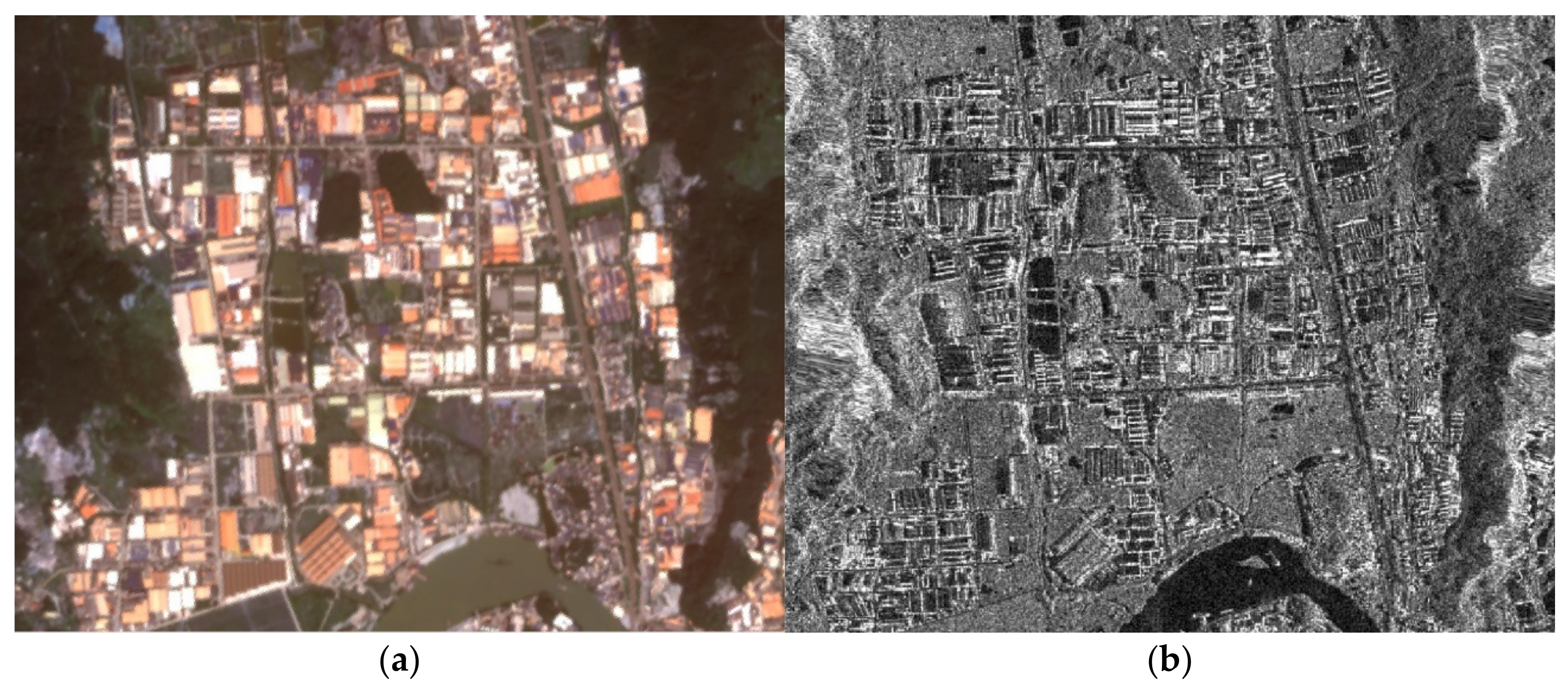
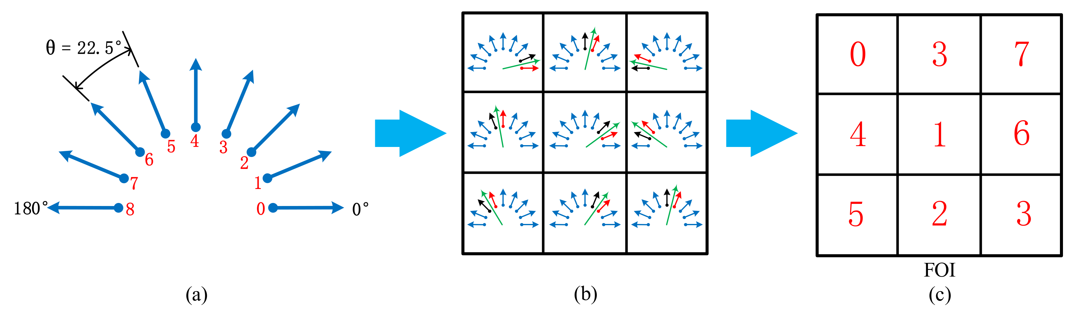
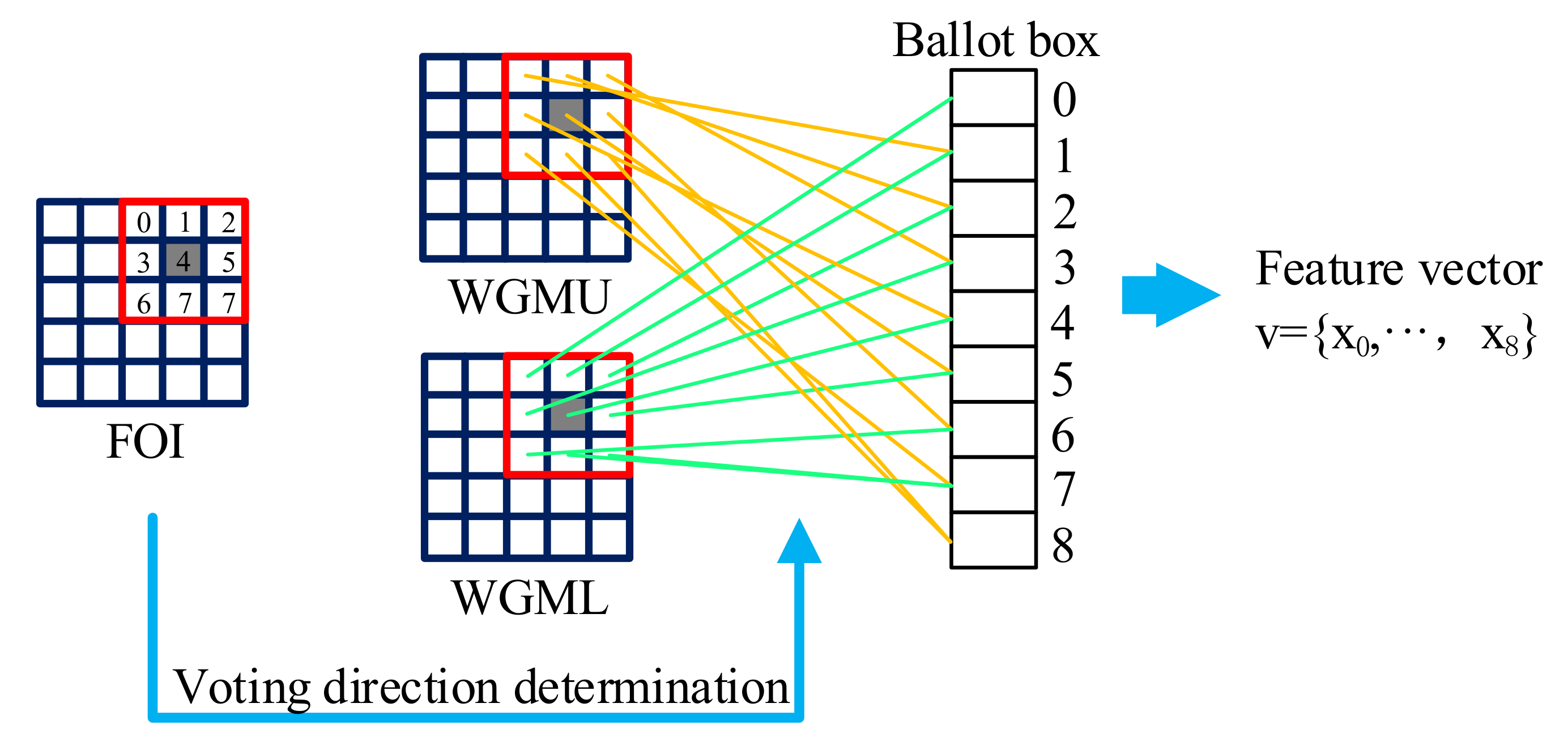
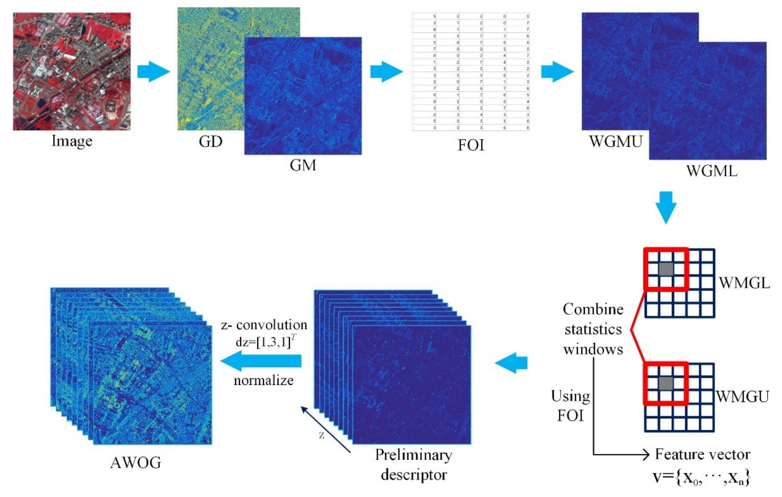
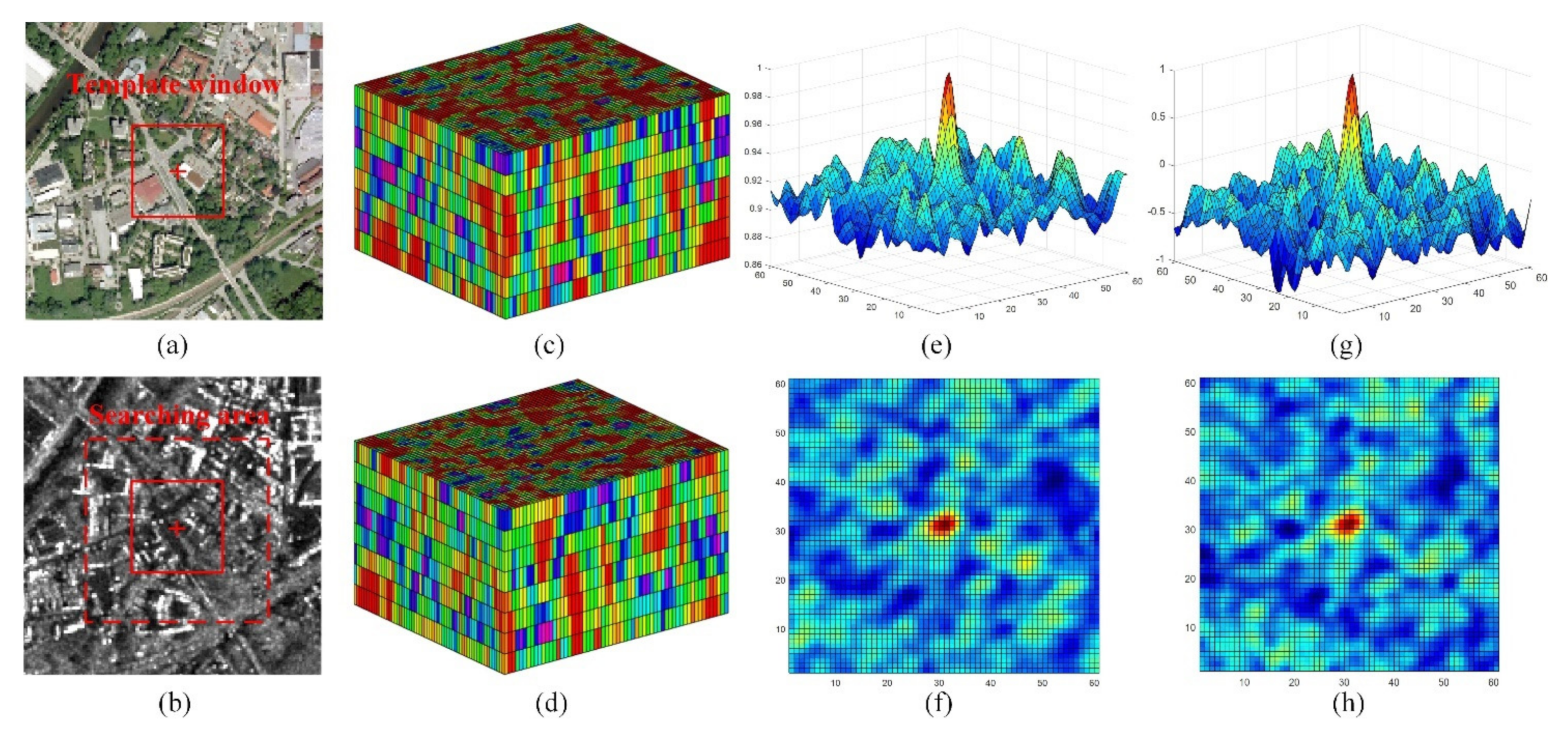
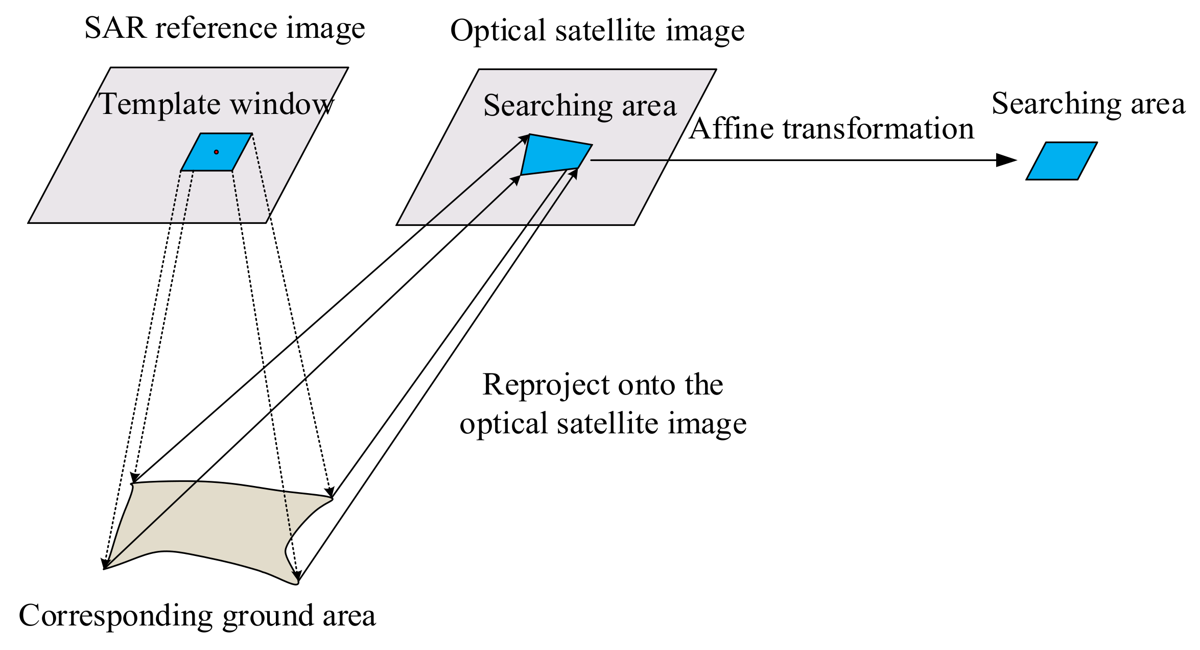
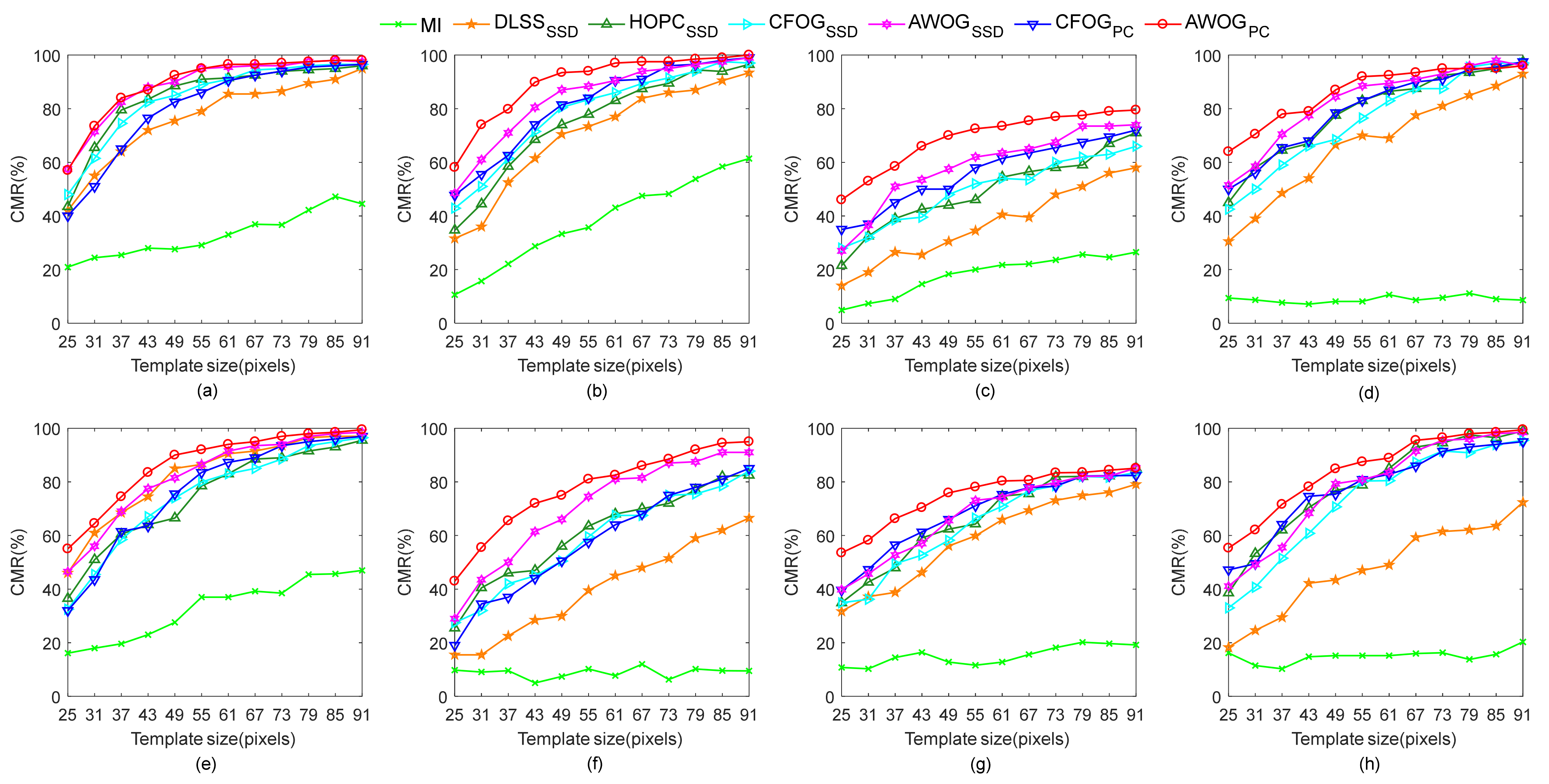
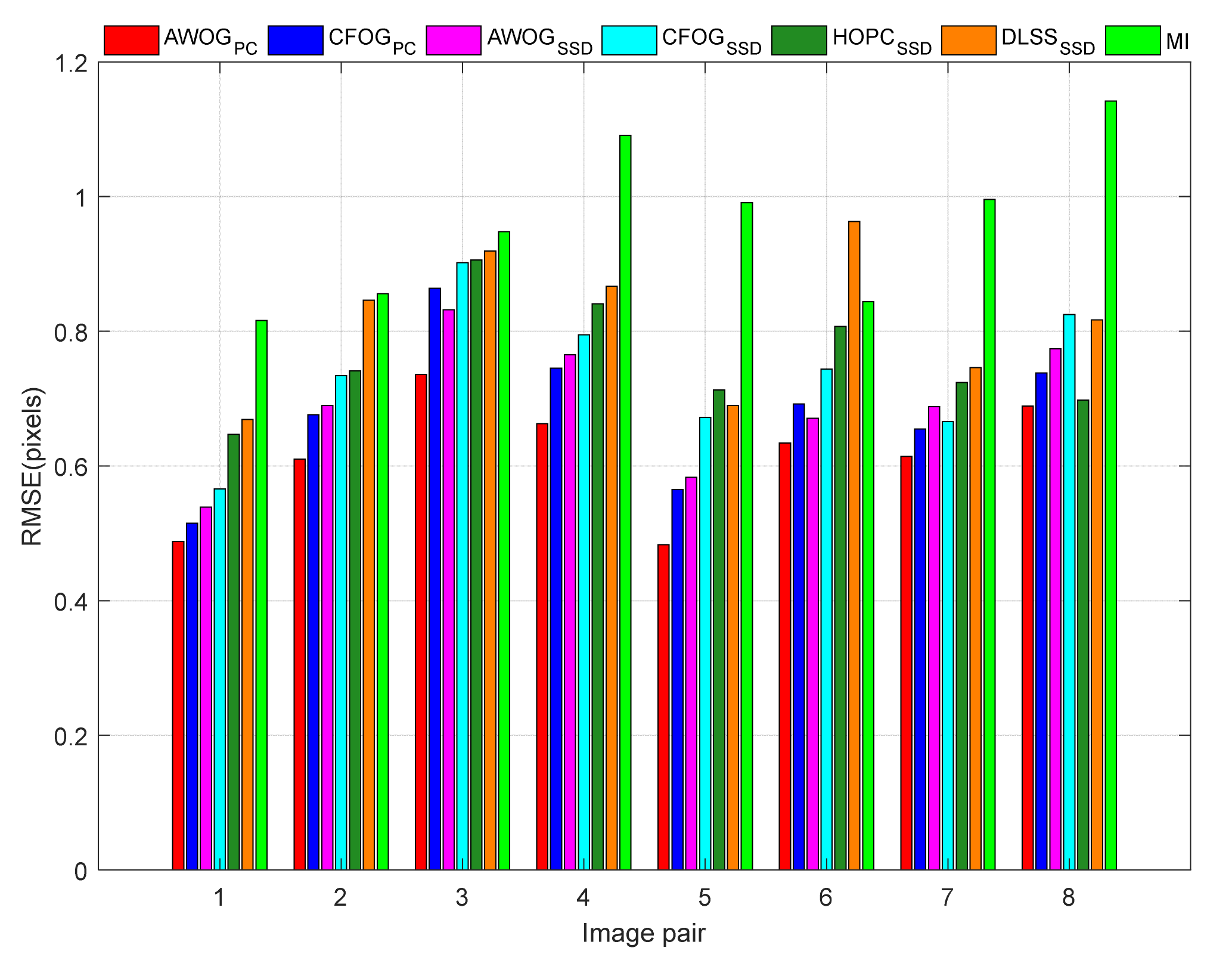
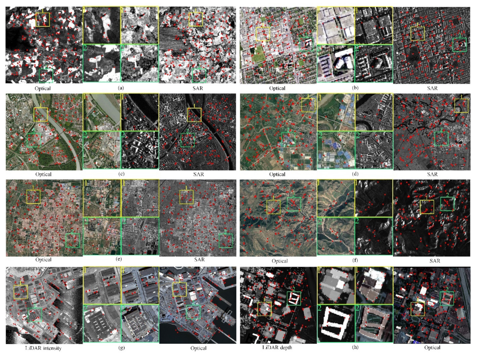
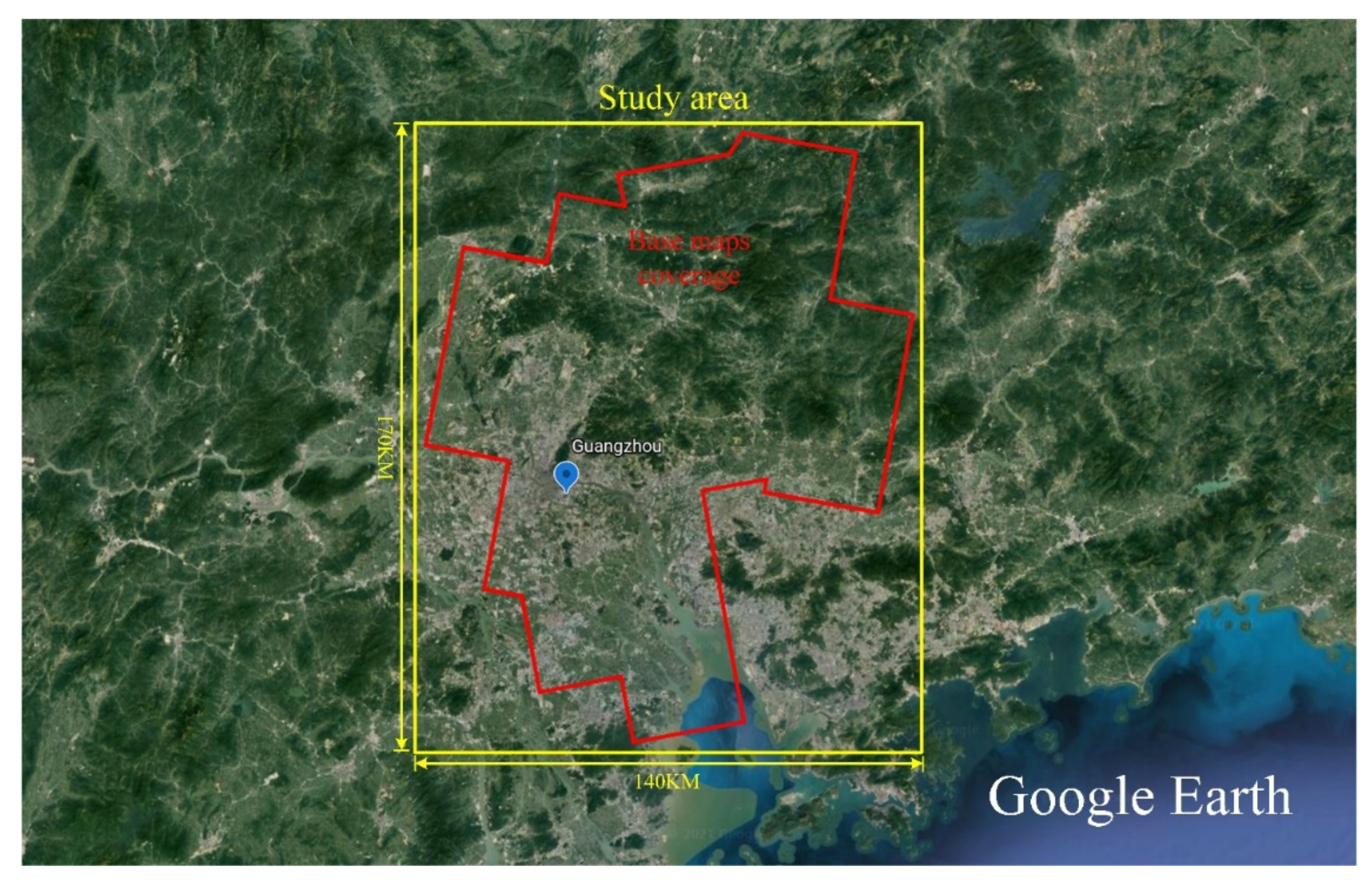
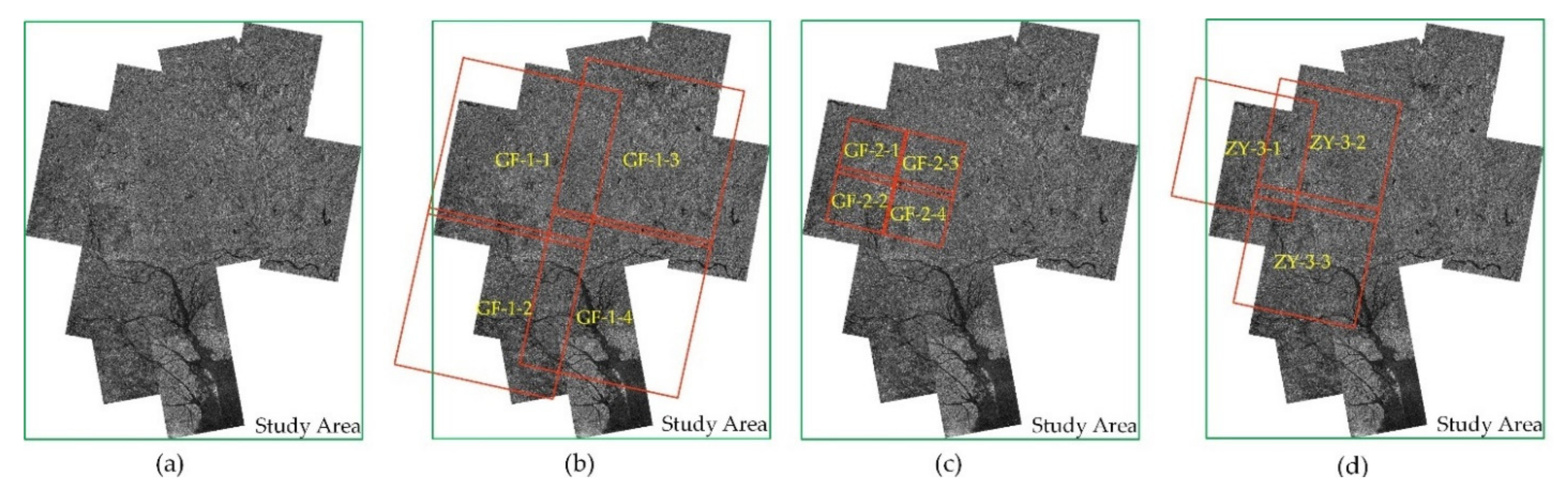
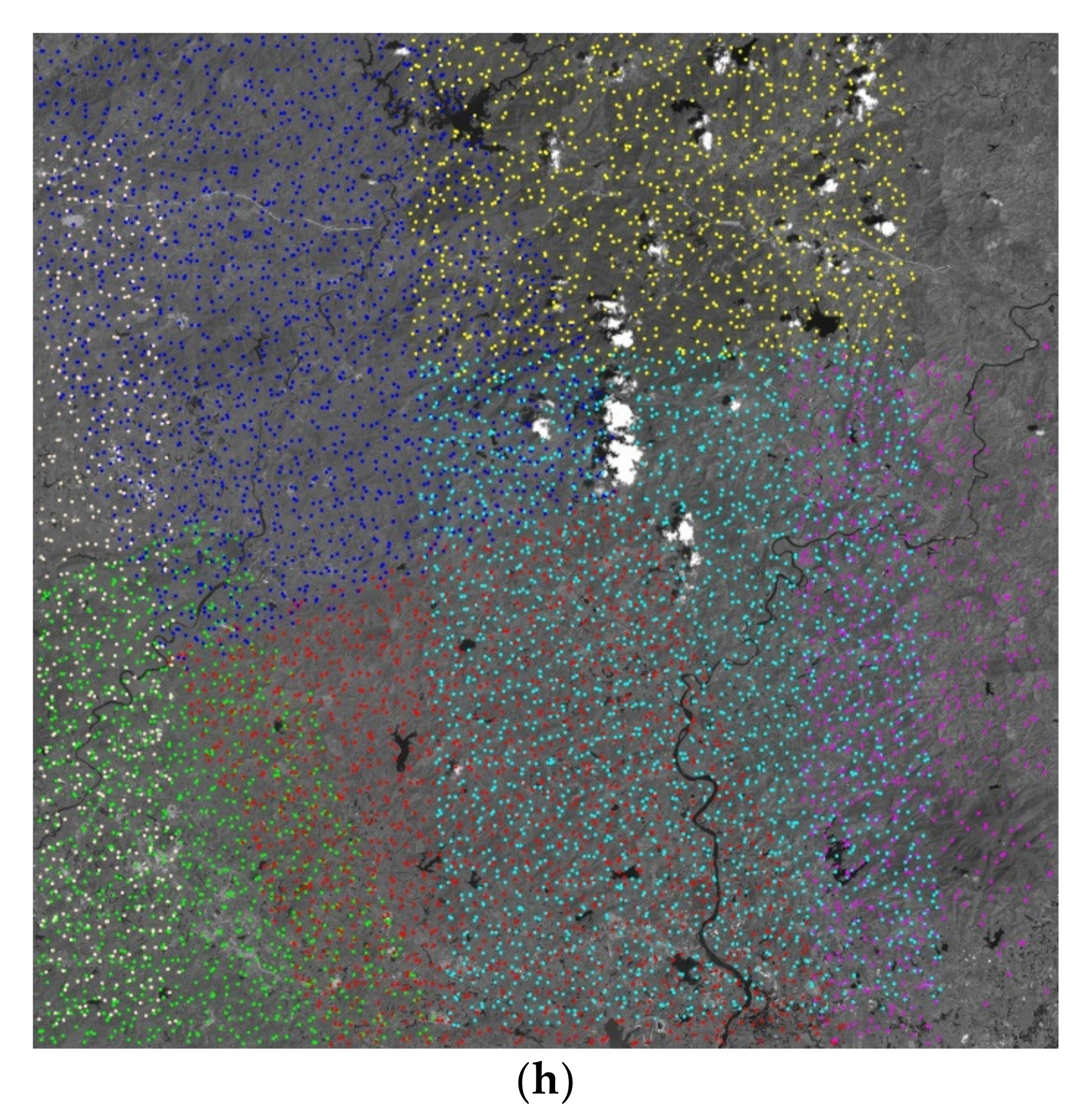
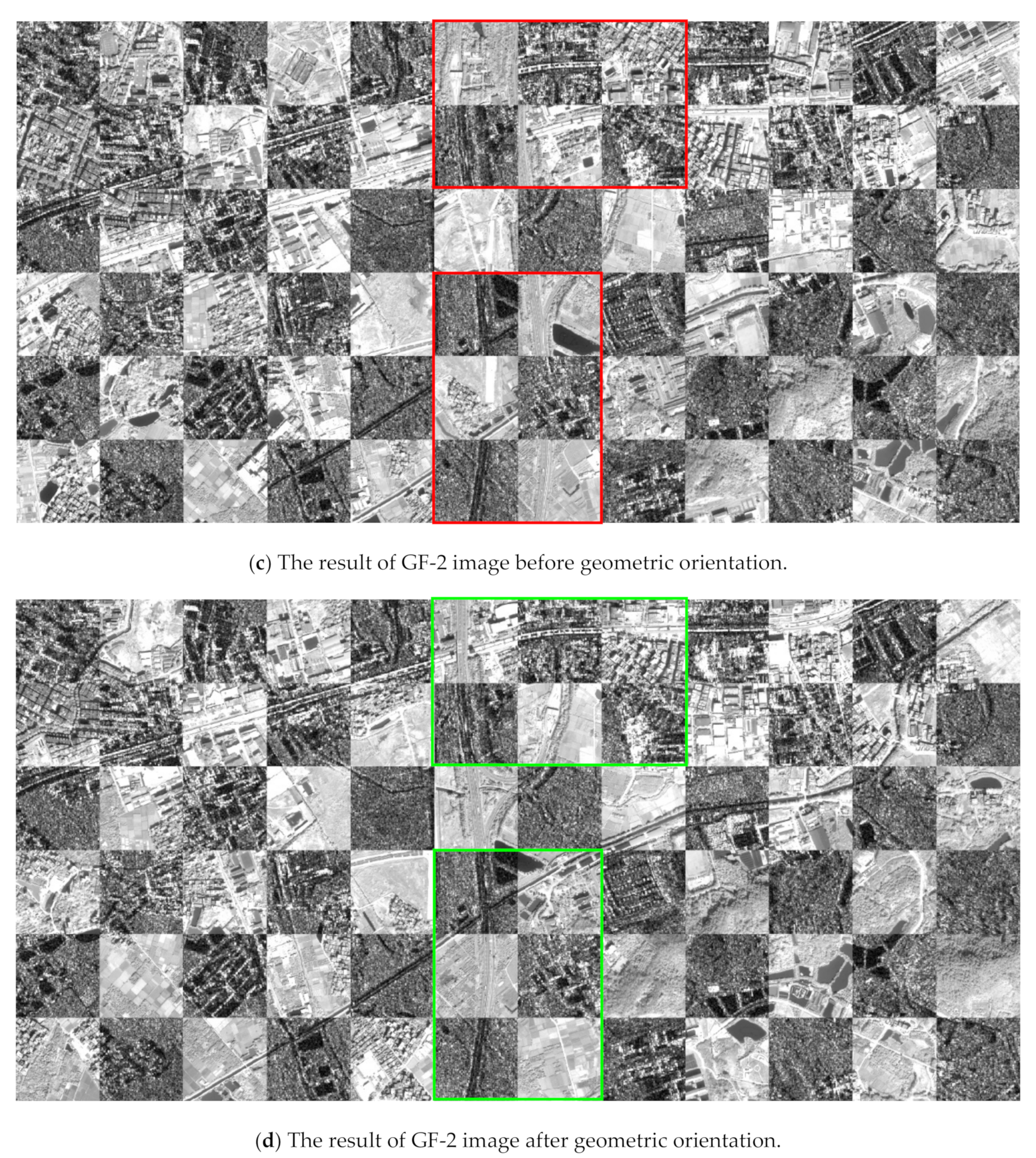
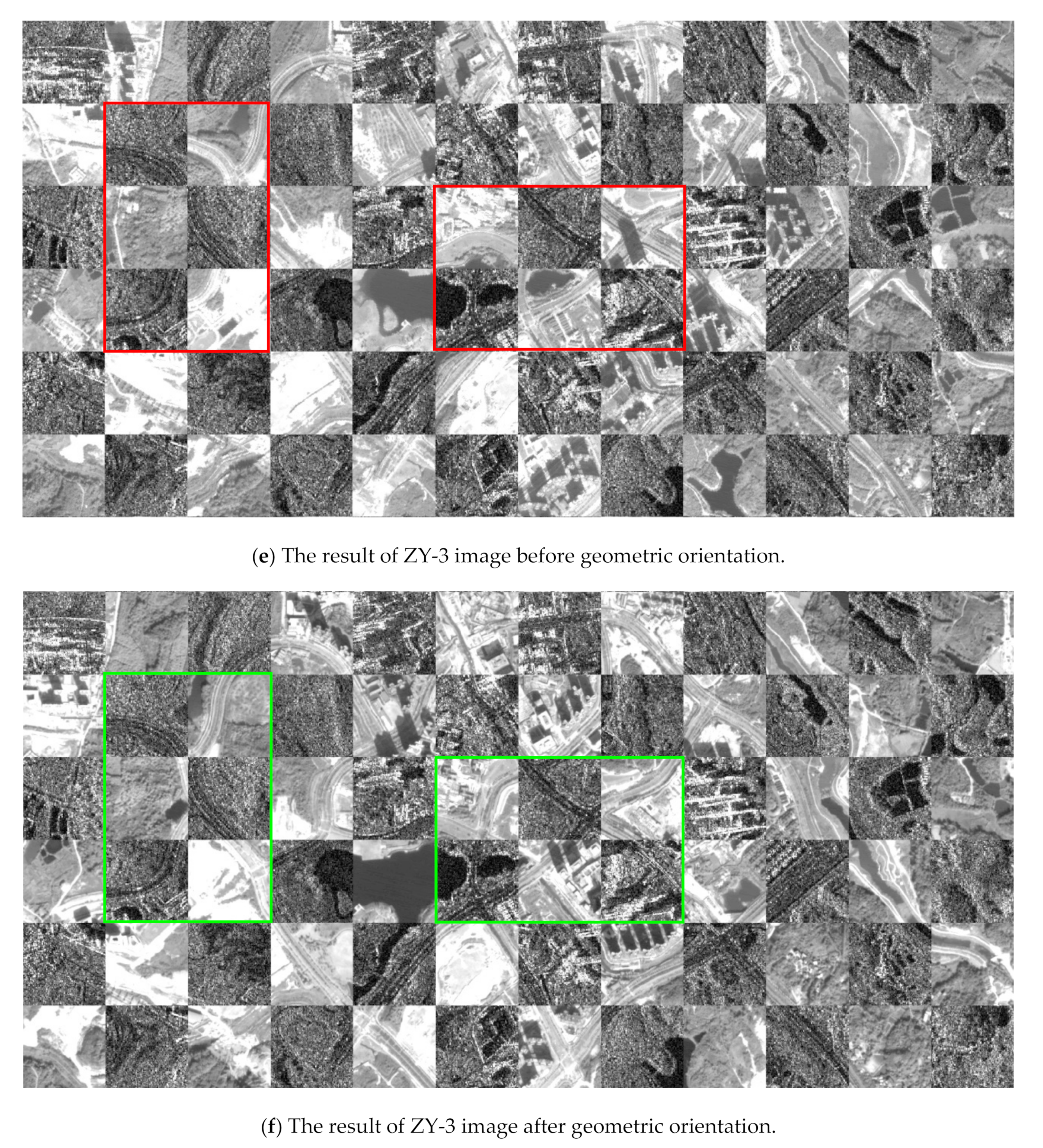
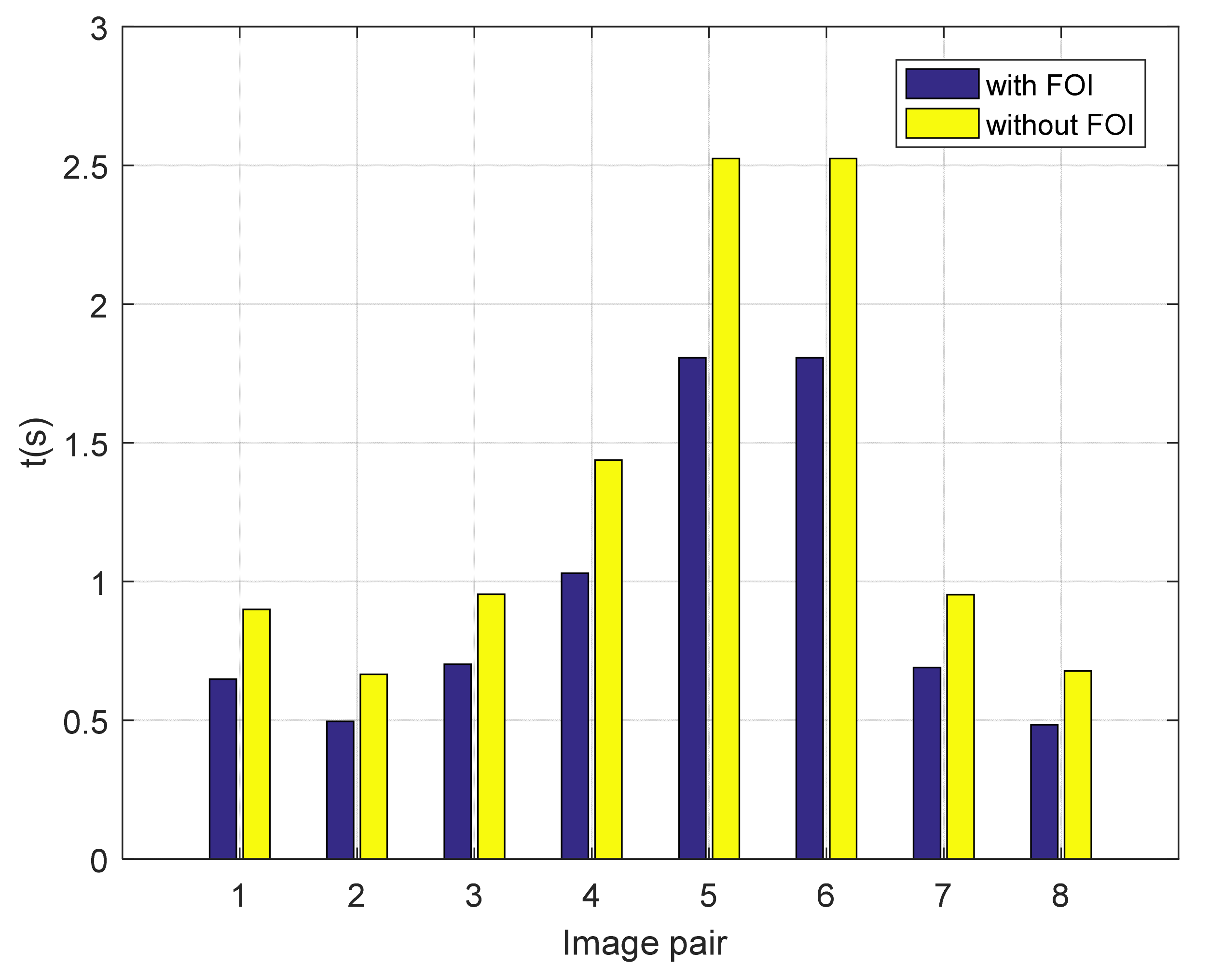
Table 1.
The detailed information of all experimental image pairs used in Section 5.1.1.
Table 1.
The detailed information of all experimental image pairs used in Section 5.1.1.
| Category | Image Pair | GSD | Date | Size (Pixels) | |
|---|---|---|---|---|---|
| Optical-to-SAR | 1 | TM band3 | 30 m | May 2007 | 600 × 600 |
| TerraSAR-X | 30 m | March 2008 | 600 × 600 | ||
| 2 | Google Earth | 3 m | November 2007 | 528 × 524 | |
| TerraSAR-X | 3 m | December 2007 | 534 × 524 | ||
| 3 | Google Earth | 3 m | March 2009 | 628 × 618 | |
| TerraSAR-X | 3 m | January 2008 | 628 × 618 | ||
| 4 | Google Earth | 10 m | April 2019 | 777 × 737 | |
| TH-2 | 10 m | August 2019 | 777 × 737 | ||
| 5 | Google Earth | 10 m | June 2019 | 1001 × 1001 | |
| TH-2 | 10 m | December 2019 | 1000 × 1000 | ||
| 6 | Google Earth | 10 m | August 2017 | 1001 × 1001 | |
| GF-3 | 10 m | February 2017 | 1000 × 1000 | ||
| LiDAR-to-Optical | 7 | LiDAR intensity | 2 m | October 2010 | 621 × 617 |
| WorldView-2 | 2 m | October 2011 | 621 × 621 | ||
| 8 | LiDAR depth | 2.5 m | June 2012 | 524 × 524 | |
| Airborne optical | 2.5 m | June 2012 | 524 × 524 | ||
Table 2.
The detailed RMSE values of all methods with a template window of 91 × 91 pixels.
| Image Pair | Criteria | AWOGPC | CFOGPC | AWOGSSD | CFOGSSD | HOPCSSD | DLSSSSD | MI |
|---|---|---|---|---|---|---|---|---|
| 1 | RMSE (pixels) | 0.488 | 0.515 | 0.539 | 0.566 | 0.647 | 0.669 | 0.816 |
| 2 | RMSE (pixels) | 0.610 | 0.676 | 0.690 | 0.734 | 0.741 | 0.846 | 0.856 |
| 3 | RMSE (pixels) | 0.736 | 0.864 | 0.832 | 0.902 | 0.906 | 0.919 | 0.948 |
| 4 | RMSE (pixels) | 0.663 | 0.745 | 0.765 | 0.795 | 0.841 | 0.867 | 1.091 |
| 5 | RMSE (pixels) | 0.483 | 0.565 | 0.583 | 0.672 | 0.713 | 0.690 | 0.991 |
| 6 | RMSE (pixels) | 0.634 | 0.692 | 0.671 | 0.744 | 0.807 | 0.963 | 0.844 |
| 7 | RMSE (pixels) | 0.614 | 0.655 | 0.688 | 0.666 | 0.724 | 0.746 | 0.996 |
| 8 | RMSE (pixels) | 0.689 | 0.738 | 0.774 | 0.825 | 0.698 | 0.817 | 1.142 |
Table 3.
The detailed average running times of all methods under different sizes of template windows.
Table 3.
The detailed average running times of all methods under different sizes of template windows.
| Template Size (Pixels) | Criteria | AWOGPC | CFOGPC | AWOGSSD | CFOGSSD | HOPCSSD | DLSSSSD | MI |
|---|---|---|---|---|---|---|---|---|
| 25 × 25 | t (s) | 1.279 | 0.510 | 3.019 | 1.428 | 2.446 | 2.601 | 10.011 |
| 31 × 31 | t (s) | 1.369 | 0.605 | 4.125 | 2.459 | 2.808 | 2.727 | 11.051 |
| 37 × 37 | t (s) | 1.397 | 0.610 | 4.830 | 3.061 | 2.966 | 2.854 | 12.124 |
| 43 × 43 | t (s) | 1.410 | 0.616 | 6.040 | 4.003 | 3.252 | 3.016 | 14.056 |
| 49 × 49 | t (s) | 1.425 | 0.622 | 7.065 | 4.615 | 4.105 | 3.751 | 15.582 |
| 55 × 55 | t (s) | 1.532 | 0.752 | 7.896 | 5.150 | 4.852 | 4.210 | 16.992 |
| 61 × 61 | t (s) | 1.548 | 0.766 | 9.042 | 5.908 | 6.348 | 4.601 | 17.726 |
| 67 × 67 | t (s) | 1.574 | 0.784 | 10.343 | 6.732 | 6.792 | 5.583 | 18.885 |
| 73 × 73 | t (s) | 1.591 | 0.802 | 11.612 | 7.453 | 7.193 | 5.985 | 20.421 |
| 79 × 79 | t (s) | 1.606 | 0.839 | 12.955 | 8.222 | 8.020 | 6.396 | 22.324 |
| 85 × 85 | t (s) | 1.640 | 0.860 | 14.238 | 8.988 | 9.684 | 6.969 | 24.637 |
| 91 × 91 | t (s) | 1.652 | 0.888 | 15.866 | 10.307 | 10.546 | 7.788 | 27.753 |
Table 4.
The detailed information of all experimental image pairs used in Section 5.2.1.
Table 4.
The detailed information of all experimental image pairs used in Section 5.2.1.
| Category | Sensor | GSD | Date | Amount | Average Size (Pixels) |
|---|---|---|---|---|---|
| SAR reference images | TerraSAR-X | 5 m | September 2017 | 12 | 7737 × 9235 |
| Optical satellite images | GF-1 | 2 m | September 2018 | 4 | 40,124 × 39,872 |
| GF-2 | 1 m | Noverber 2016 | 4 | 29,428 × 28,000 | |
| ZY-3 | 2 m | Decenber 2017 | 3 | 30,422 × 30,016 |
Note: the size of the images acquired by the same sensor may be slightly different, and therefore we use the average size in the table.
Table 5.
The quantitative experimental results of all experimental images.
| Image Name | Nr | No | RMSE (Pixels) | t (s) |
|---|---|---|---|---|
| GF-1-1 | 6 | 6883 | 1.05 | 87.89 |
| GF-1-2 | 5 | 4794 | 1.18 | 73.79 |
| GF-1-3 | 7 | 9046 | 0.86 | 98.18 |
| GF-1-4 | 7 | 5799 | 0.93 | 93.07 |
| GF-2-1 | 2 | 897 | 1.67 | 33.15 |
| GF-2-2 | 3 | 923 | 1.61 | 43.98 |
| GF-2-3 | 3 | 1581 | 1.45 | 42.88 |
| GF-2-4 | 3 | 1469 | 1.68 | 43.47 |
| ZY-3-1 | 3 | 2310 | 1.06 | 45.91 |
| ZY-3-2 | 5 | 5216 | 0.81 | 67.54 |
| ZY-3-3 | 6 | 5269 | 1.10 | 78.31 |
Nr means the number of reference SAR images that the optical satellite image could use for orientation. No means the number of output VCPs. RMSE represents the location error between the optical satellite image and SAR reference images after the geometric orientation process. t means the running time.
Table 6.
The experimental results with a fixed and different parameter settings of .
| Criteria | = 3 | ||||
|---|---|---|---|---|---|
| = 3 | = 5 | = 8 | = 9 | = 10 | |
| CMR/% | 94.5 | 96.2 | 96.5 | 96.0 | 96.0 |
| RMSE/pixels | 0.691 | 0.619 | 0.606 | 0.604 | 0.601 |
| t/s | 0.941 | 0.978 | 1.091 | 1.144 | 1.189 |
Table 7.
The experimental results with a fixed and different parameter settings of .
| Criteria | = 8 | ||||
|---|---|---|---|---|---|
| = 3 | = 5 | = 7 | = 9 | = 11 | |
| CMR/% | 96.5 | 96.0 | 92.5 | 84.7 | 76.2 |
| RMSE/pixel | 0.606 | 0.635 | 0.697 | 0.718 | 0.726 |
| t/s | 1.091 | 1.189 | 1.379 | 1.626 | 1.955 |
Publisher’s Note: MDPI stays neutral with regard to jurisdictional claims in published maps and institutional affiliations. |
© 2021 by the authors. Licensee MDPI, Basel, Switzerland. This article is an open access article distributed under the terms and conditions of the Creative Commons Attribution (CC BY) license (https://creativecommons.org/licenses/by/4.0/).
Share and Cite
MDPI and ACS Style
Fan, Z.; Zhang, L.; Liu, Y.; Wang, Q.; Zlatanova, S. Exploiting High Geopositioning Accuracy of SAR Data to Obtain Accurate Geometric Orientation of Optical Satellite Images. Remote Sens. 2021, 13, 3535. https://doi.org/10.3390/rs13173535
AMA Style
Fan Z, Zhang L, Liu Y, Wang Q, Zlatanova S. Exploiting High Geopositioning Accuracy of SAR Data to Obtain Accurate Geometric Orientation of Optical Satellite Images. Remote Sensing. 2021; 13(17):3535. https://doi.org/10.3390/rs13173535
Chicago/Turabian StyleFan, Zhongli, Li Zhang, Yuxuan Liu, Qingdong Wang, and Sisi Zlatanova. 2021. "Exploiting High Geopositioning Accuracy of SAR Data to Obtain Accurate Geometric Orientation of Optical Satellite Images" Remote Sensing 13, no. 17: 3535. https://doi.org/10.3390/rs13173535
Note that from the first issue of 2016, this journal uses article numbers instead of page numbers. See further details here.