‘The Best of Two Worlds’—Combining Classifier Fusion and Ecological Models to Map and Explain Landscape Invasion by an Alien Shrub

Abstract

The spread of invasive alien species promotes ecosystem structure and functioning changes, with detrimental effects on native biodiversity and ecosystem services, raising challenges for local management authorities. Predictions of invasion dynamics derived from modeling tools are often spatially coarse and therefore unsuitable for guiding local management. Accurate information on the occurrence of invasive plants and on the main factors that promote their spread is critical to define successful control strategies. For addressing this challenge, we developed a dual framework combining satellite image classification with predictive ecological modeling. By combining data from georeferenced invaded areas with multispectral imagery with 10-meter resolution from Sentinel-2 satellites, a map of areas invaded by the woody invasive Acacia longifolia in a municipality of northern Portugal was devised. Classifier fusion techniques were implemented through which eight statistical and machine-learning algorithms were ensembled to produce accurate maps of invaded areas. Through a Random Forest (RF) model, these maps were then used to explore the factors driving the landscape-level abundance of A. longifolia. RF models were based on explanatory variables describing hypothesized environmental drivers, including climate, topography/geomorphology, soil properties, fire disturbance, landscape composition, linear structures, and landscape spatial configuration. Satellite-based maps synoptically described the spatial patterns of invaded areas, with classifications attaining high accuracy values (True Skill Statistic, TSS: 0.895, Area Under the Receiver Operating Curve, ROC: 0.988, Kappa: 0.857). The predictive RF models highlighted the primary role of climate, followed by landscape composition and configuration, as the most important drivers explaining the species abundance at the landscape level. Our innovative dual framework—combining image classification and predictive ecological modeling—can guide decision-making processes regarding effective management of invasions by prioritizing the invaded areas and tackling the primary environmental and anthropogenic drivers of the species’ abundance and spread.

1. Introduction

Biological invasions represent a major threat to biodiversity worldwide, with a broad range of impacts on ecosystem services, natural capital, and human well-being [1]. The introduction of alien organisms in new ecosystems has grown exponentially during the last decades due to the increase of trade (on a global scale) and unprecedented mobility of people and goods [2,3]. Driven by this reality, new and often more aggressive invasive species are expected to spread, threatening the use of natural resources.

Due to their potential impacts and associated costs, biological invasions are at the core of major global political initiatives, from the 1992 Convention on Biological Diversity (CBD) to the 2030 Agenda for Sustainable Development of the United Nations. Specific to invasions, the Aichi Target 9 from the CBD’s Strategic Plan for Biodiversity 2011-2020 stipulated that “by 2020, invasive alien species and pathways are identified and prioritized, priority species are controlled or eradicated, and measures are in place to manage pathways to prevent their introduction and establishment”. Successfully pursuing that goal over this new decade will require a stronger focus on mapping, predicting, and identifying potential risks and promoting action upon invaders before they become established [4].

Besides direct human management, the success of biological invasions is determined by three broad factors: the number of propagules entering the new environment, the new species’ life strategy and functional characteristics, and the environment’s susceptibility to invasion [5]. The invasion process is deeply influenced by the traits of receiving landscapes that promote their susceptibility to invasion by species from other world regions. Moreover, the spatial and ecological patterns of invasive plants are strongly driven by disturbance regimes acting upon ecosystems and landscapes [6].

Even though the need to enhance ecosystem services often drives plant species introductions in non-native ranges (e.g., soil fixation, erosion control, landscape aesthetics), several negative ecological, economic, and social impacts can occur if the species become invasive. In particular, woody invasive alien species can alter ecosystem processes and functions (e.g., biodiversity erosion, increased fire-proneness, allergic reactions to pollen, dense vegetation in roads or tracks, ecosystem functioning disruptions) [7,8,9].

Acacia species are known worldwide for their invasive characteristics [10]. In the northwest of Portugal (where the study area is located), environmental factors such as the regions’ rugged topography, the high levels of precipitation and sun hours, associated with anthropological factors like rural abandonment and fire regime changes during the last decades promoted the spread of several invasive plant species of the genus Acacia, including Acacia longifolia (Andrews) Willd [11,12,13] (hereafter A. longifolia).

Accurate high-resolution mapping of invasive alien species is critical to pursue political initiatives, especially for anticipating, early detection, and support management options on plant invasions [14,15], and remote sensing imagery and techniques are paramount for this purpose. Multispectral sensors onboard satellite platforms, such as Sentinel-2, improve the possibilities of detecting alien plant species not only because of suitable spatial, temporal, and spectral resolutions of the sensor array but also due to the large image swath covering vast regions at once. Another advantage of Sentinel-2 is that data is available free of charge in contrast to commercial very-high-resolution platforms such as RapidEye, WorldView-1-4, GeoEye-1, in which image acquisition costs are often impeditive for long-term monitoring. Sentinel-2 offers ten spectral bands covering the visible, near, and shortwave infrared at a spatial resolution of 10 to 20 m (plus three additional bands with 60 m resolution) and five days of temporal resolution. Such characteristics make Sentinel-2 suitable for invasive species mapping and assessment and allow continuous monitoring at several spatial and temporal scales [14]. These advances make possible a better detection and perception of the spectral and physical differences between alien plant species and autochthonous species/vegetation [15].

Complementarily to advances in remote sensing, new statistical and machine-learning algorithms allow to better exploit and profit from these data. The software package biomod2 [16] is a well-established platform implemented in R that allows users to assess and combine different modeling/classification techniques based on statistical and machine-learning algorithms [17]. Designated as an ensemble platform for species distribution modeling (SDM), biomod2 allows predicting the habitat suitability of a species across a geographic space by establishing relationships between species and environmental variables, based on statistical and machine-learning algorithms [18,19]. Despite the unquestionable value and usefulness of SDMs, they often fall short to actually depict invaded areas and characterize several dimensions usually required by policymakers who need to quickly and accurately detect invaded places to plan interventions [20]. This happens because SDMs are correlative models, calculated from species presence/absence (or pseudo-absence) point records which are then related to environmental variables (e.g., climate, geomorphology, soil, land use) to generate a final potential distribution of a target species, often with a coarse resolution inadequate for control or management efforts [21].

However, the biomod2 R package can also be applied to perform pixel-based supervised classification through an ensemble approach, which in the context of remote sensing image analysis and data mining science, is known as “classifier fusion” or “stacking” methods [22]. These techniques allow the combination of different supervised classification algorithms to obtain a final consensus capable of discriminating the presence/absence of a species based on satellite spectral data. As such, biomod2 can be used as a suitable multi-classifier stacking ensemble, which allows standardizing the uncertainty present in the individual models and determines a general prediction consistent with all classification methods [16,23]. Another advantage of combining spectral data in biomod2 for alien plant species mapping relates to its ability to run non-parametric models that, unlike parametric models, can assume that a pixel is a mixture of features and sub-divide each one to increase spectral variance inside and between pixels [24].

In addition to fast-paced advances in remote sensing satellite platforms and accessibility of its data, predictive models in ecology, and especially in invasion biology (e.g., [9,25]) are also growing and diversifying their applications. Predictive modeling is the process of applying a statistical model or machine-learning algorithm to data to predict an outcome or to capture the association between the outcome (e.g., presence/absence or abundance of a species) and a set of drivers as defined by [26]. This analytical toolkit, supported mainly by statistical and machine-learning algorithms, allows for inferences regarding multi-scale invasion drivers (either invasibility or invasiveness) and obtain spatiotemporal predictions [8]. Overall, these advances manifest in managers’ and stakeholders’ ability to profit from the availability of data and analytical routines to make better assessments, monitor, and devise strategies to control invasive species. Despite these advances, the combination of both satellite image classification (for invasive species mapping/detection) and predictive modeling (for inferring invasion drivers) has been seldom explored (but see, e.g., [27]). As such, researchers miss the ability to profit from synergistic advances of both fields and obtain more insights regarding species invasions.

Aiming to address this gap, in this study we developed and tested a dual methodological framework for assessing landscape invasion by alien woody plants. The framework is illustrated for landscape invasion by the Golden wattle (Acacia longifolia) in a municipality of Northern Portugal. First, we developed an improved mapping approach based on Sentinel-2 imagery and stack fusion techniques with the R package biomod2 to generate a spatially explicit representation of invaded areas. Secondly, we used a predictive model-based procedure with the Random Forests algorithm to assess the influence on the invasion process of several hypothesized drivers related to (i) (bio-)climate, (ii) topography/geomorphology, (iii) soil properties, (iv) fire disturbance, (v) land use/landscape composition, (vi) linear landscape elements, and (vii) landscape pattern/configuration. We discuss the relevance of the proposed approach—combining satellite image classification and predictive ecological modeling—to manage invasive alien species at an appropriate scale to guide decision-making processes.

2. Materials and Methods

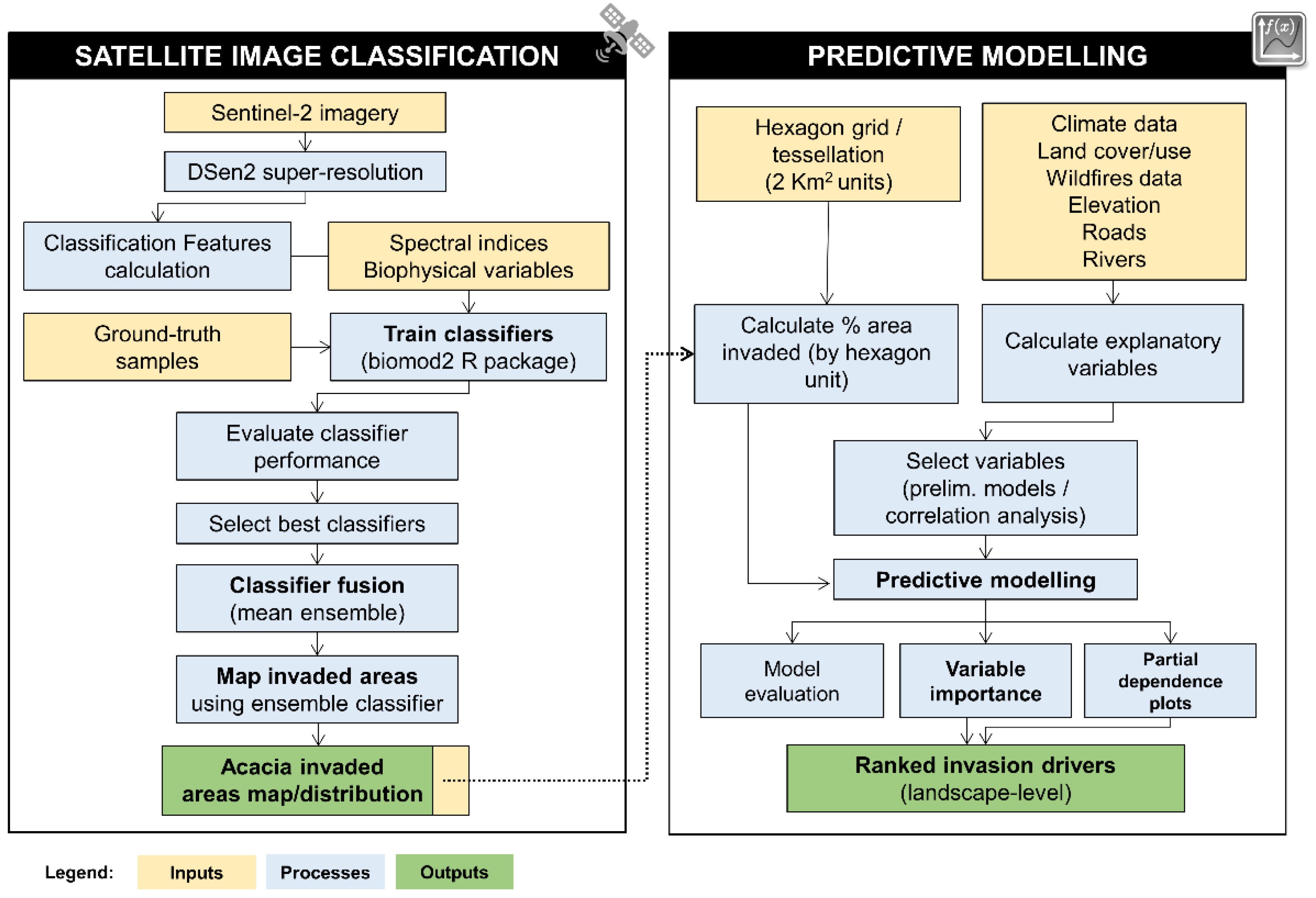
2.1. General Workflow

To address the challenges of mapping the invasive alien plant species A. longifolia and identify the key drivers underlying the spread and abundance at the landscape level, we propose and develop a dual approach. In stage one (see Section 2.5, Section 2.6, Section 2.7, Section 2.8), supervised image classification (supported by classifier fusion) was used to map the extent of invasion by the target species based on Sentinel-2 data. In stage two (see Section 2.9), predictive modeling was used to underpin and rank the importance of the main drivers of the species invasion. This last component of the workflow relied on a landscape-level approach, supported by previous results from stage one (i.e., invaded areas map) and a hexagon tessellation of the whole study area. This workflow enabled us to assess which environmental factors, and respective drivers, mainly contribute to the spread of the species. Specific steps of each stage are described in Figure 1 and detailed in the subsections below.

2.2. Target Species

In general, Australian Acacia species are known for their phenotypic plasticity and invasive abilities, promoting a wide range of impacts, causing a general reduction in ecosystem services delivery [28]. These species spread impacts on public health (e.g., allergies) [29,30], decrease in the water availability (either by the traits of the plant or by the density) [31], modification on the biogeochemical cycles [32,33,34], homogenization of ecosystems composition and structure [35], change of fire regimes and competition with native species [10].

Specifically, the target species A. longifolia was introduced in Portugal for ornamental purposes and for fixing soils in eroded areas [36]. In particular, this species is known to spread along the coastline, degraded areas, and through the margins of low-altitude rivers. Together with the increasing human pressure in these specific areas, the resilience and natural value has severely decreased [37,38]

Due to A. longifolia traits, such as rapid growth, regeneration capacity (sprouting vigorously), reaction to disturbing agents (fire), remarkable ability to compete for resources, production of viable seeds for decades, absence of competitors and natural predators, this species is an aggressive invader in the study area [39].

2.3. Study Area

The study area is located in the municipality of Viana do Castelo (NW Portugal), which has an area of 319.02 km² and 85,445 inhabitants. The region presents a temperate climate, with an average annual temperature of 14.5 °C and an average annual rainfall of 1264 mm [40]. With a remarkable geomorphological and landscape heterogeneity marked by three distinct landscape units: mountain, riverside, and coastline, its rugged topography (from sea level to a maximum elevation above 800 m) make this region unique for its diversity and specific habitat types associated with high levels of biodiversity [40].

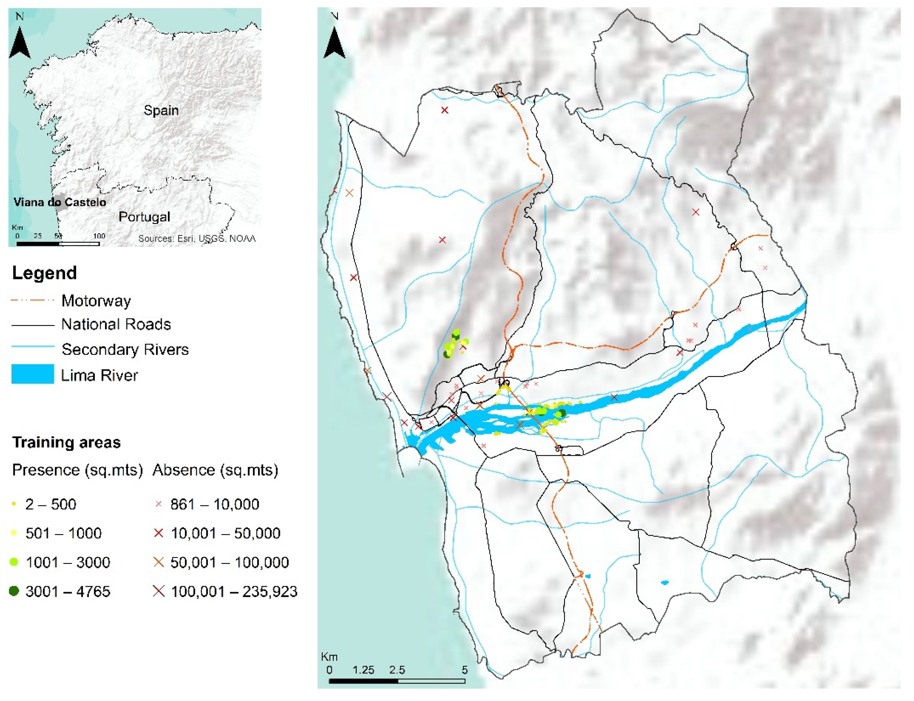
In the study area, A. longifolia is spread in large areas, some of them classified as Natura 2000, causing ecological impacts and promoting ecological regime changes (e.g., alteration of the forest composition of riparian galleries) [41]. Furthermore, the study area presents a set of socio-ecological conditions which facilitate the species expansion, such as the current regime of very frequent rural fires, large seed banks, and a very dense corridor network (associated with communication roadways) (Figure 2).

2.4. Occurrence Data

The delimitation of training areas is of great importance for obtaining accurate results. The biomod2 classification algorithms are characterized by having binomial responses (distribution values between 0 and 1), where 0’s code absences of A. longifolia and 1’s denotes its presence. The diversity of natural spaces and their land uses creates several challenges for identifying spatial and spectral signatures for A. longifolia.

To represent the environmental heterogeneity on the study area, a total of 207 training areas were considered, covering river margins, mountainous areas, seaside, and urbanized spaces, always having the attention to record especially significant training areas (i.e., combining mixed pixels but most often heavily invaded areas which generate ‘pure’ pixels for training). Several sites representing the study area’s main land cover types (e.g., urban, forest, motorway, shrublands, and agricultural areas) were inspected to collect training samples. Through ground surveys and GPS equipment, sites invaded with considerable dimensions (>5 m²) were recorded and georeferenced (n = 67). Due to some locations’ inaccessibility, GIS tools and orthophoto maps with high-spatial-resolution (0.3 m) were used to obtain additional presence areas (n = 100). Additionally, through manual photointerpretation of high-resolution images, several areas representing the main land cover types for the study area were collected and used as absences (i.e., ‘true-absences’; n = 40). The overall median size of training areas is 188 m², while the median size of presence areas is 112 m² and 13,820 m² for absence areas.

To better represent the spectral variance in the image stack and complement the data from true-absences, three sets of pseudo-absences were randomly generated throughout the study area using biomod2’s internal routines. To balance train data and avoid biasing the accuracy of model predictions [42], the number of pseudo-absences was set equal to the number of presences.

2.5. Satellite Remote Sensing Data

Sentinel-2A multispectral data, provided by the Copernicus Open Access Hub, was analyzed and inputted in the classification workflow. We collected one image per month between December 2018 to May 2019, covering the final stage of the growing season (December–January), flowering period (January–March), and post-flowering period (April–May). To increase accuracy, it is necessary to minimize overall cloud cover in collected images from the study area. For each of the six days analyzed, we collected imagery with 13 spectral bands (Top-Of-Atmosphere Level L1C) that were transformed into the atmospherically corrected L2A product through the sen2cor processing software for better comparability, spectral quality, and increased signal retrieval [43], thus creating 12 available bands.

Through the DSen2 super-resolution algorithm [44], the spectral bands at 20 and 60 m were resampled to 10 m through a pre-trained deep neural network implementing this method, attaining better performance than standard resampling methods [44]. The improved and rescaled bands were then used to calculate, for each month, several spectral vegetation indices: Normalized Difference Vegetation Index (NDVI), Enhanced Vegetation Index (EVI), Modified Chlorophyll Absorption in Reflectance Index (MCARI), MERIS Terrestrial Chlorophyll Index (MTCI), and the second Modified Soil Adjusted Vegetation Index (MSAVI2). For higher accuracy on the vegetation index calculation, specific formulas for Sentinel-2A bands were employed [45] (

Table 1. List of spectral vegetation indices and biophysical variables used to support A. longifolia supervised classification and mapping.

Index	Explanation	Specific Formula
NDVI	Enhances vegetation differences photosynthetically [46]	$\frac{\left(\mathrm{b}8 - \mathrm{b}4\right)}{\left(\mathrm{b}8 + \mathrm{b}4\right)}$
EVI	Distinguish differences in the canopy structure, architecture, and physiognomy [47,48]	$2.5\frac{\mathrm{b}9 - \mathrm{b}5}{\left(\mathrm{b}9 + 6\mathrm{b}5 - 7.5\mathrm{b}1\right) + 1}$
MCARI	A measure of the leaf chlorophyll content enhancing vegetation differences [49]	$\left(\left(\mathrm{b}5 - \mathrm{b}4\right) - 0.2\left(\mathrm{b}5 - \mathrm{b}3\right)\right)\left(\frac{\mathrm{b}5}{\mathrm{b}4}\right)$
MTCI	Enhances vegetation senescence and water/nutritional stress [50]	$\frac{\left(\mathrm{b}6 - \mathrm{b}5\right)}{\left(\mathrm{b}5 + \mathrm{b}4\right)}$
MSAVI 2	Retrieves information about vegetation dynamics and reduced the soil background variations [51]	$\frac{2\mathrm{b}9 + 1 - \surd \left(2\mathrm{b}9 + 1\right)2 - 8\left(\mathrm{b}9 - \mathrm{b}5\right)}{2}$
LAI	Measure for the total area of leaves per unit ground area [52]	S2 SNAP Toolbox biophysical processor.

).

The Leaf Area Index (LAI) was calculated through the software SNAP with the original 12 bands. In total, 18 spectral layers (12 bands and 6 indexes) were considered for each month (totaling n = 108).

2.6. Biomod2 Multi-Algorithm Supervised Classification Training and Evaluation

The study was performed using the latest version of the biomod2 package (version 3.4.6) within the statistical software R (R Development Core Team 2012) version 4.0. This analysis is supported by several supervised classification algorithms, based either on statistical or machine learning methods, including Generalized Linear Model (GLM), Flexible Discriminant Analysis (FDA), Gradient Boosting Machine (GBM), Random Forest (RF); Classification Tree Analysis (CTA), Generalized Linear Model (GAM), Artificial Neural Network (ANN), and MAXENT, Phillips (MAX).

For the input dataset, three different sets of pseudo-absences and 30 model repetitions were performed using the default options of biomod2. For evaluating the performance of the classifiers, holdout cross-validation was used by setting 80% of the dataset for training and 20% for evaluation purposes. Additionally, we ensured a prevalence of 0.5, which means that the presences and the pseudo-absences have the same weight in the model calibration process.

To evaluate the overall performance of either partial and final ensemble/fusion classifiers for the test fraction (i.e., not used for training), we calculated the True-Skill Statistic (TSS), Cohen’s Kappa (KAPPA), and the area under the Receiver Operating Curve (ROC). The first two measures vary from [−1, 1] while the second between [0, 1]. Values closer to one flag better-performing classifiers and higher discrimination ability. To complement these measures, we also calculated sensitivity and specificity. Sensitivity is the proportion of observed presences predicted and, therefore, quantifies omission errors, while specificity is the proportion of observed absences that are correctly predicted and therefore quantifies commission errors. Overall, sensitivity is the probability that the classification algorithm will correctly classify presences, whereas specificity is the probability that the model will correctly classify absences.

2.7. Variable Reduction and Importance Calculation

Considering that biomod2 demands considerable computational resources, especially when the number of variables (or features) used is high, a preliminary reduction was performed. To identify critical variables in the model’s preparation and thus reduce the total number of variables, we analyzed the importance of each through a set of preliminary modeling steps using six classification techniques: GLM, FDA, GBM, RF, CTA, and MAX. Variable importance calculation was performed using biomod2’s function variables importance, which returns each variable’s importance score. The highest the value, the more influence the variable has on the supervised classification process. A value of 0 assumes no influence of a variable, whereas values closer to 1 signal a highly important variable [17]. This variable importance analysis allowed selecting the variables with higher importance, making the classifier fusion less computationally demanding [53]. We considered the best 17 individual variables to maintain a good ratio between performance and complexity (Appendix A).

2.8. Classifier Fusion Ensemble

An ensemble fusion model was obtained by calculating the weighted mean (by the TSS performance score) of selected partial classifiers, i.e., those which got a good to excellent performance considering a rule of TSS > 0.8. Finally, to convert the ensemble classifier model result from probability/suitability values (i.e., continuous values within the [0, 1] range) to a binary outcome (species presence: 1 or absence: 0), we applied a numerical threshold [54,55]. In our case, we defined this “binarization” threshold as the value which maximizes the TSS score [56].

Values lower than the TSS cutoff were considered pixels with very low spectral similarity to invaded areas, whereas biomod2’s output values close to the maximum rescaled probabilistic value of 1000 were considered to have very-high spectral similarity to invaded areas.

2.9. Assessing the Invasion Drivers of A. longifolia at the Landscape Level through Predictive Modelling

From the classified Sentinel-2A images, we assessed the abundance drivers of A. longifolia through a predictive model-based framework based on the Random Forest regression algorithm [57]. We started by devising a hexagonal grid (or tessellation) covering the whole study area with 2 Km² units for performing this assessment. This grid was necessary to adequately address the structural and environmental drivers promoting the abundance of A. longifolia at the landscape level. The size of each hexagonal unit was considered suitable for three relevant criteria: (i) maximize the environmental heterogeneity, (ii) scale conformity to climate data (which is the coarser dataset with ~1 Km² of spatial resolution), and (iii) adequate sample size for modeling (n = 189 effective units after checking for invalid data).

The response variable is the proportion covered by invaded areas for each hexagon unit, obtained from zonal statistics of the classified Sentinel-2A imagery from previous steps. The A. longifolia map generated through image classification was used to quantify the response variable, allowing to get a full area view of invasion extent at the landscape level instead of relying on a limited set of sample training areas for that purpose.

The list of predictive drivers (

Table 2. Full list of environmental factors considered, which were hypothesized as drivers of invasion in the study area, totaling 59 independent variables (see also Appendix B). Variables in bold were selected for the final RF regression model (n = 20).

Environmental Factors	Driver Description	Acronym
(Bio)Climate	Annual Mean Temperature	CL_BIO01
	Mean Diurnal Range	CL_BIO02
	Isothermality	CL_BIO03
	Temperature Seasonality	CL_BIO04
	Maximum Temperature of Warmest Month	CL_BIO05
	Minimum Temperature of Coldest Month	CL_BIO06
	Temperature Annual Range	CL_BIO07
	Mean Temperature of Wettest Quarter	CL_BIO08
	Mean Temperature of Driest Quarter	CL_BIO09
	Mean Temperature of Warmest Quarter	CL_BIO10
	Mean Temperature of Coldest Quarter	CL_BIO11
	Annual Precipitation	CL_BIO12
	Precipitation of Wettest Month	CL_BIO13
	Precipitation of Driest Month	CL_BIO14
	Precipitation Seasonality	CL_BIO15
	Precipitation of Wettest Quarter	CL_BIO16
	Precipitation of Driest Quarter	CL_BIO17
	Precipitation of Warmest Quarter	CL_BIO18
	Precipitation of Coldest Quarter	CL_BIO19
Disturbance	Total Burnt Area (last 10 years)	DT_BA10YR
	Total Burnt Area (last 20 years)	DT_BA20YR
	Total Burnt Area (last 5 years)	DT_BA5YR
Land use	Percent of permanent crops	LU_PCPCO
	Percent of annual crops	LU_PCACO
	Percent of permanent and annual crops	LU_PCPAC
	Percent of native forests	LU_PCNFO
	Percent of eucalyptus (production) forest	LU_PCEFO
	Percent of maritime-pine (production) forest	LU_PCPFO
	Percent of shrublands	LU_PCSHL
	Percent of complex agroforestry mosaics	LU_PCAFM
	Percent of other production forests	LU_PCOPF
	Percent of pasturelands	LU_PCPAS
	Percent of wetlands	LU_PCWET
	Percent of beaches and sand dunes	LU_PCBSD
	Percent of roads and rails	LU_PCRRL
	Percent of bare rock surfaces	LU_PCBRS
	Percent of water surfaces	LU_PCWTS
	Percent of artificial/urban areas	LU_PCART
	Percent of sparsely vegetated areas	LU_PCSPV
Landscape pattern/configuration and heterogeneity	Landscape Mean Patch Area	LP_MNPAR
	Landscape Patch Area Coefficient of variation	LP_PACOV
	Landscape Largest Patch Index	LP_LAPAI
	Landscape Shannon Diversity	LP_SHDVI
	Landscape Simpson Diversity	LP_SPDVI
	Landscape Patch Area Standard-deviation	LP_PASTD
Linear elements	Landscape edge density	LE_EDGDN
	Total length of rivers	LE_TLRIV
	Total length of all road types	LE_TLROD
	Total length of motorways	LE_TLMTW
Soil properties	Available water content	SO_AVWTC
	Bulk Density	SO_BULKD
	Percent of clay in soils	SO_PCLAY
	Percent of coarse elements in soils	SO_PCOAR
	Percent of sand in soils	SO_PSAND
	Percent of silt in soils	SO_PSILT
Topography/Geomorphology	Slope (%)	TG_SLOPE
	Average Solar Radiation	TG_RADAV
	Topographic Ruggedness Index	TG_TORGI
	Topographic Wetness Index	TG_TOWTI

), exploits the following aspects of distribution and colonization of A. longifolia at the landscape level, which relate to the degree of invasibility [8].

To select a smaller and meaningful set of predictive drivers, we performed an iterative variable elimination procedure combining variable importance obtained from an initial set of Random Forest models (n = 500) and multicollinearity reduction through non-parametric Spearman correlation analysis. From this analysis, we retained the 20 most important drivers with a pairwise correlation of ρ < |0.75|. This number of drivers was chosen to include at least one variable from each of the seven groups of drivers (see Appendix B for the complete list).

Model evaluation, for the final model including the selected set of predictive drivers, was based on the Out-Of-Bag (OOB) fraction [57,58], which consists of the subset of records not selected for training through bootstrap resampling in RF. Based on this, the following evaluation metrics were calculated: R-squared (R²), Spearman Correlation (CORSP), Root-Mean-Square Error (RMSE) and, the Median Absolute Error (MAE).

Drivers’ importance ranking was assessed through multiple runs of RF (n = 1000) and calculating the percentage increase in mean square error by shuffling the OOB samples’ values. For each tree, the prediction error on OOB samples is calculated through the mean-square error. After that procedure, the same is performed after permuting each predictor driver. The difference between the two is then averaged over all trees and normalized by the standard deviation of the differences to obtain the final importance measure. Importance values across all rounds were averaged. To increase the random forest model interpretability, we developed partial dependence plots [59], which can be defined as low-dimensional graphical representations of the prediction function so that the relationship between the outcome and each predictor can be more easily visualized and interpreted. These plots are especially useful for explaining the output of “black-box” models such as the random forest model.

3. Results

The results obtained supported the spatially explicit detection of areas invaded by A. longifolia. The supervised image classification performance through biomod2’s revealed a good ability to map the target species.

Preliminary analysis aiming to reduce the number of variables employed in the image classification stage allowed for some performance gains while also making it less demanding in computation time. The results obtained by the variable importance analyzes can be consulted in Supplementary Information—Tables S1 and S2. In addition, the development of a predictive model based on the mapping carried out in the first stage, and the main environmental variables allowed identifying drivers of invasibility.

3.1. Partial and Ensemble Fusion Classification Performance

The supervised classification technique with the best results for all evaluation metrics was GAM, followed by the FDA and RF algorithms. In contrast, the classification technique ANN presented the lowest scores across all classifiers (

Table 3. Partial evaluation scores by classification algorithm showing the average and standard deviation (across evaluation rounds). Numbers in bold indicate the top-three algorithms in our study.

	TSS		ROC		KAPPA
Classification Algorithm	Average	Standard Deviation	Average	Standard Deviation	Average	Standard Deviation
GBM	0.799	0.042	0.953	0.014	0.796	0.042
RF	0.824	0.043	0.962	0.012	0.823	0.043
CTA	0.715	0.045	0.886	0.027	0.715	0.045
GLM	0.789	0.068	0.928	0.051	0.800	0.069
FDA	0.827	0.030	0.964	0.009	0.831	0.030
ANN	0.640	0.057	0.859	0.033	0.646	0.057
MAX	0.726	0.045	0.890	0.025	0.731	0.045
GAM	0.843	0.031	0.965	0.011	0.846	0.030

). On average, across all partial classifiers, we found high-performance scores with 0.794 for TSS, 0.945 for ROC, and 0.798 for KAPPA.

Overall, the ensemble classifier based on biomod2’s multi-algorithm fusion showed very high-performance values as well as sensitivity and specificity (

Table 4. Performance evaluation scores for the final ensemble classifier combining biomod2 algorithms.

Evaluation Metric	Evaluation Metric Value (Test)	Cutoff Threshold	Sensitivity	Specificity
TSS	0.895	539	96.0	93.4
ROC	0.988	544	96.0	93.5
KAPPA	0.857	724	88.7	96.7

). The ensemble model presents a performance gain for any evaluation metric value compared to the best partial classification model (i.e., GAM). This gain shows the added value of fusing multiple classifiers with distinct types of algorithmic frameworks (i.e., such as tree-based in CTA or RF vs. neural networks in ANN).

3.2. Feature Importance in Image Classification

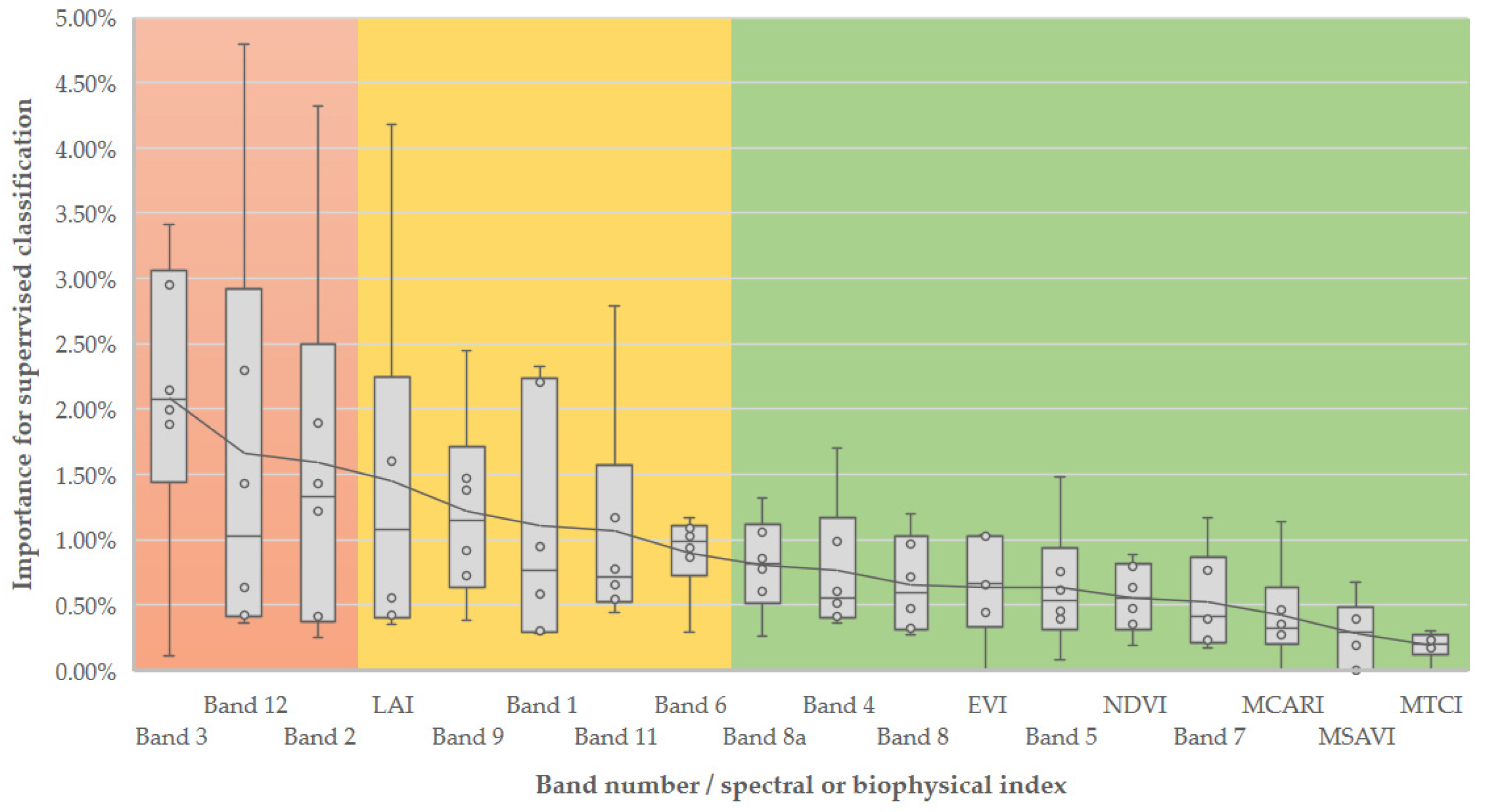
According to biomod2 ranking, the four most important variables were Band 3 (green), Band 12 (SWIR2), Band 2 (blue), and the LAI index. In opposition, the bands with lower importance were in the spectral region of red (band 4), red edge (bands 5, 6 and, 7), and the near infrared (bands 8 and 8a), often used for remote sensing of vegetation. Overall, the variable importance analysis highlighted the usefulness of the spectral bands on the classifier (with 78% of all information used) in contrast to the less performant vegetation and biophysical indices (with 22%) (Figure 3). Despite exhibiting lower importance scores and secondary contributions, the remaining variables also improved overall accuracy.

The selection of the most important variables (to reduce the computational processing time) resulted in 17 layers of spectral information with a combined relative importance of approximately 45%. The three most important independent variables were band 12 (SWIR band 2) in December (4.79%), band 2 (blue) in January (4.32%), and LAI in January with (4.18%).

The months with the highest combined relative importance (from the 17) were December, January, February (Appendix A), which coincides with the final growing period and the flowering period. On the other hand, April and May were the months with smaller contributions to the classification process (Figure 4).

3.3. Acacia Longifolia Mapping

The ensemble classifier based on the biomod2’s ensemble fusion approach was able to discriminate invaded areas by A. longifolia spectrally similar to training sites. These areas occur along the Lima and Minho River (with higher density when approaching estuarine spaces), coastal areas, low altitude slopes with high solar exposure and smooth inclination, and discontinuous urban areas (Figure 5).

The distribution pattern A. longifolia, in the study area, coincides primarily with spaces of high ecological value under protection networks (e.g., Natura 2000).

3.4. Predictive Modelling—Landscape-Level Drivers of A. longifolia Invasion

After performing the preliminary models and correlation analyses, 20 predictive drivers were selected to include in the final model out of 59 (see Supplementary Information—Table S3 for all variable importance rankings). These drivers are for the climate the Temperature Seasonality (CL_BIO04), Minimum Temperature of the Coldest Month (CL_BIO06), Precipitation Seasonality (CL_BIO15), and Precipitation of the Warmest Quarter (CL_BIO18). For topography/geo-morphology, it includes Average Solar Radiation (TG_RADAV), while for soil properties, the available water content (SO_AVWTC), percentage of clay (SO_PCLAY), and percentage of coarse elements (SO_PCOAR). As for disturbance, solely the Total Burnt Area in the last five years (DT_BA5YR) was selected. Land use and landscape composition include the percentage of annual crops (LU_PCACO), percentage of eucalyptus (production) forest (LU_PCEFO), percentage of maritime-pine (production) forest (LU_PCPFO), percentage of other types of production forest (LU_PCOPF), percentage of shrublands (LU_PCSHL) and percentage of artificial/urban areas (LU_PCART) while for linear structures the Total length of rivers (LE_TLRIV) and, Total length of motorways (LE_TLMTW) and, finally, for landscape pattern/configuration the Landscape Mean Patch Area (LP_MNPAR), Simpson’s Landscape Diversity (LP_SPDVI), and the Patch Area Coefficient of variation (LP_PACOV).

Overall, model performance for the selected drivers was generally good for the OOB test fraction with a coefficient of determination R² of 0.52 and a Spearman correlation between predicted and observed values of 0.76. The MAE and RMSE have an error between 3.8 and 5.5% which is considered acceptable given the response variable distribution (min: 0.0%, max: 57.5%, mean: 7.3%, standard deviation: 7.7%).

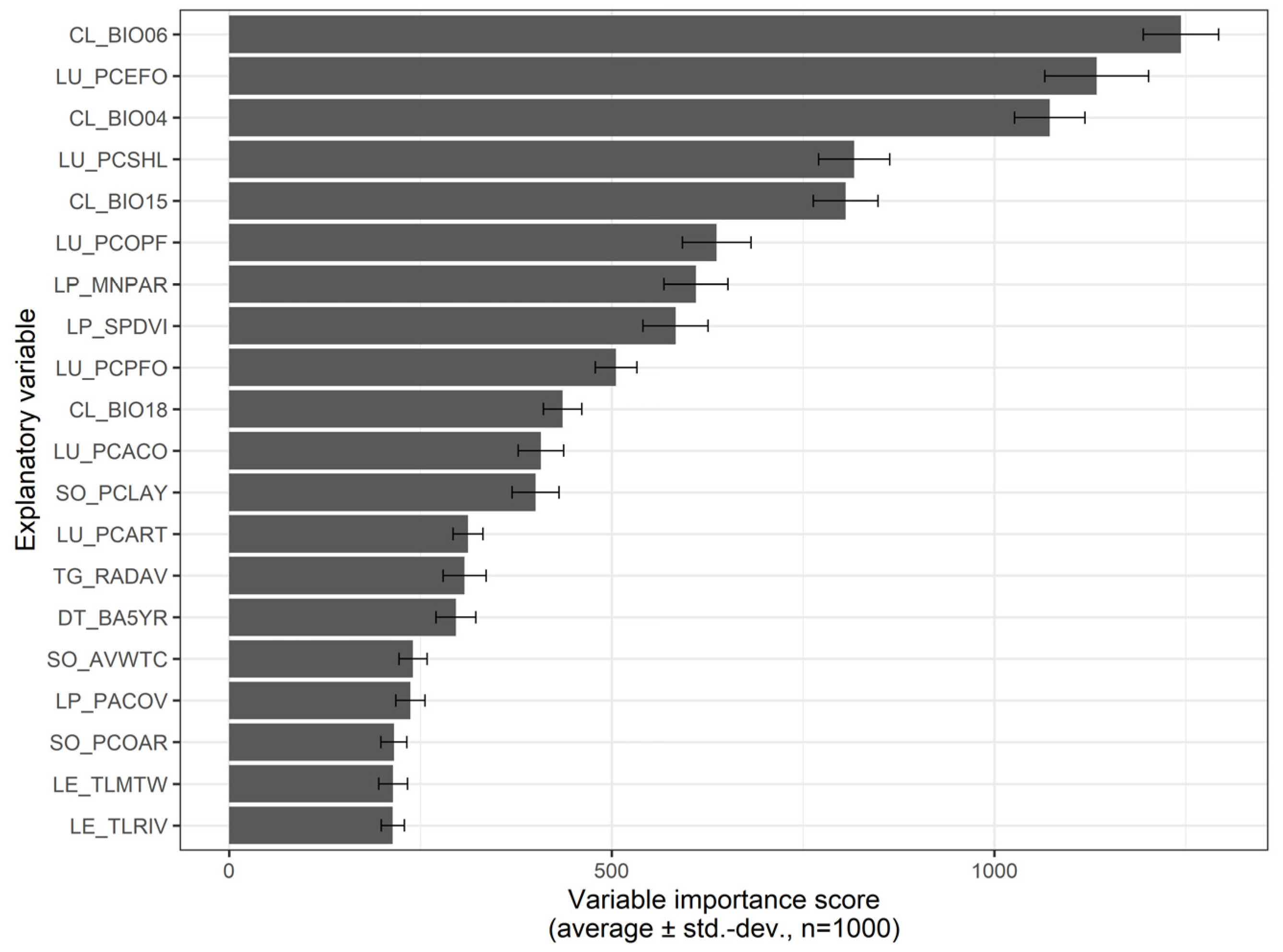
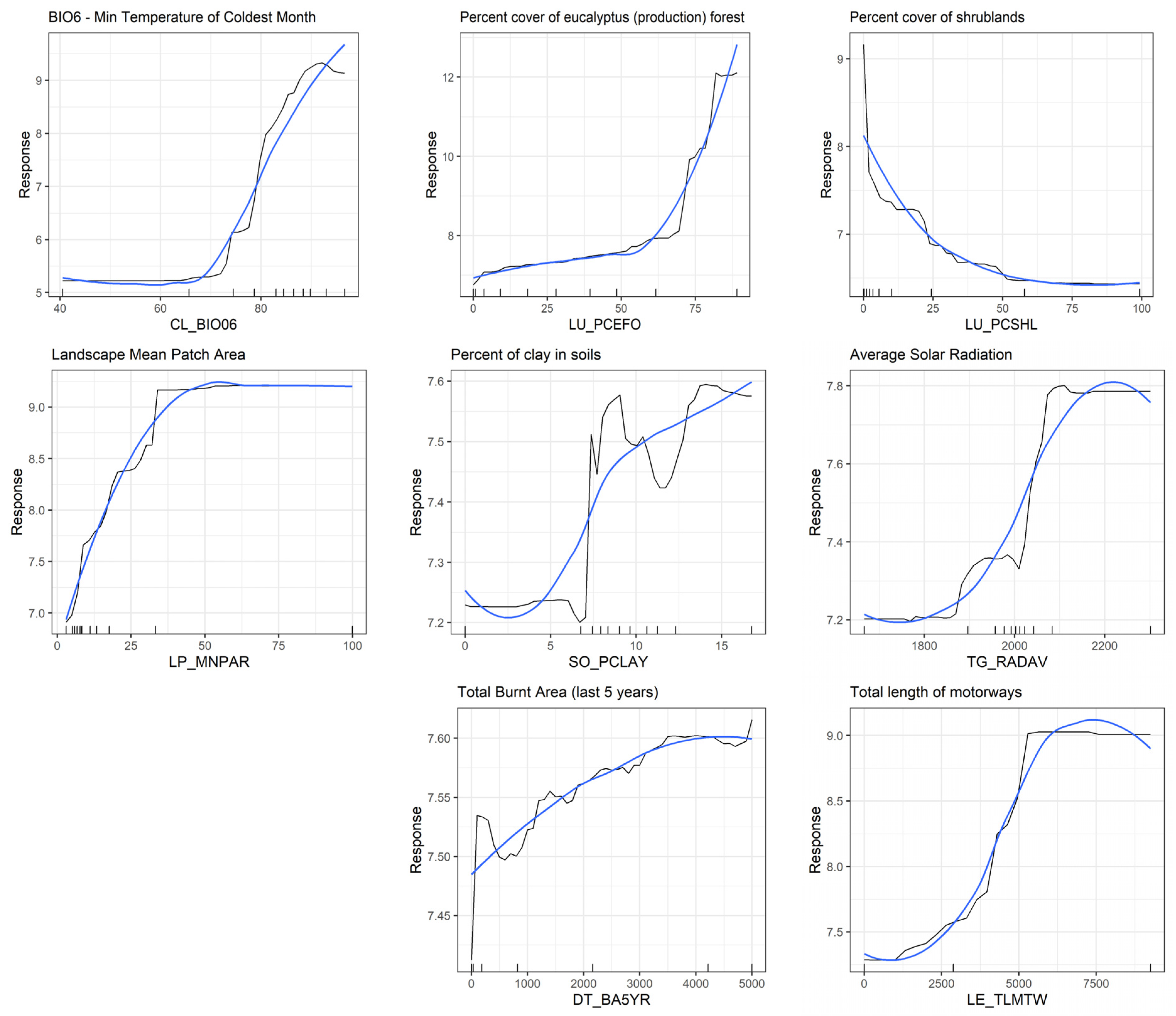
The random forest model importance (Figure 6) allowed ranking the selected drivers, which highlighted first the role of climate followed closely by land use and landscape spatial configuration (see Supplementary Information—Table S4 for driver importance ranking for the 20-best selected). We found that drivers related to soil properties, topography, disturbance, and linear elements in the landscape had comparatively less importance. Besides importance scores, partial dependence plots (Figure 7) allowed us to deepen the interpretation of each predictive driver of A. longifolia invasion extent at the landscape level.

More specifically, invaded areas were positively related to higher annual minimum temperature values and higher precipitation seasonality and negatively associated with temperature seasonality and the precipitation of the warmest/summer quarter (see Figure 7 and Supplementary Information—Figure S1 for all plots).

For land use/landscape composition, production forests of all types (i.e., eucalyptus, pine, and other less common types), which dominate the tree strata in invaded areas, were all positively related to invaded areas. In contrast, shrublands and annual crops were negatively related. Artificial areas showed a complex response, with invaded areas peaking at small values (i.e., probably related to forest-like landscapes) and again increasing at high values (i.e., urbanized landscape as the dominant matrix with semi-natural habitats dispersed).

As for landscape pattern/configuration, highly invaded areas tend to have larger patches (potentially dominated by continuous forest areas of a single type, e.g., monocultures of eucalyptus, maritime pine, or other dominant tree species). This effect can also be observed in the Simpson Landscape Diversity index, which is negatively related to the percentage cover of invaded areas, showing that less heterogeneous areas create favorable conditions for the target species spread.

In terms of soil attributes, the species was positively related to soils with higher clay content and a lower percentage of coarse elements. Solar radiation (which is modulated by topography and exposure) was positively associated with the species. Disturbance dynamics related to wildfires (calculated as the total burnt area in the five past years) positively contributed to species abundance. Linear elements traversing the landscape, including both natural features (i.e., rivers) and artificial ones (i.e., motorways), also showed positive effects contributing to the landscape-level abundance of A. longifolia.

4. Discussion

4.1. Multispectral Remote Sensing Imagery and Data Fusion Techniques through biomod2 for A. longifolia Detection

Although distribution maps of invasive alien plants are common in scientific literature, due to the requirements and the fine-scale of species-level mapping, most resort to very-high-resolution satellites (≤5 m), airborne or unoccupied aerial vehicles to collect remote sensing data [60,61]. These data and techniques are often associated with considerable economic investments, low temporal resolutions, and time-demanding procedures (both in personal and computational terms). Spatially explicit maps of invasive alien plants are critical to understanding their spatiotemporal distribution patterns and their driving factors at several scales to support and improve management and control strategies.

For tackling this challenge, satellite remote sensing coupled with classifier fusion methodologies (such as the one employed here through the biomod2 R package) offers tremendous advantages [62]. First, this methodology is implemented on the R computing platform, firmly established in the academic community. Second, multispectral and multitemporal high-resolution imagery is free of charge (e.g., Sentinel-2, Landsat), allowing continuous updates of invasive alien plant species’ distribution maps. Moreover, contrary to species distribution models, which target invasive alien plant potential distribution, satellite image classification does not require environmental variables at low spatial resolution (e.g., precipitation; temperature).

Our study showed the ability of Sentinel-2 to support invasive alien plant mapping through a multitemporal approach supported by multispectral data together with vegetation and biophysical indices stacks, capable of feeding the biomod2 fusion classifier. Overall, results show that the spatial, spectral, and temporal resolutions of Sentinel-2 were adequate for mapping A. longfiolia invaded areas, and it may be the case for similar plant species sharing similar compositional and structural traits [52].

However, contrary to what one would expect, the primary source of spectral information was not in the red, red-edge, or near-infrared regions (often valuable for depicting spectral information about concentrations of chlorophyll-a and other pigments typically used for vegetation analyses [52]). The Sentinel-2′s blue (458–523 nm), green (543–578 nm), and SWIR2 (2100–2280 nm) spectral bands were those that showed, for our study region and the period analyzed, better ability to discriminate between A. longifolia and other woody species.

A possible explanation for this fact is that A. longifolia fluorescence, like other yellow flowers, is better distinguished at the spectrum comprehend between 480–550 nm [63]. The carotenoids (yellow pigments) are known to cause high reflectance on the spectral region covered by the green light (due to decreased chlorophyll absorption of red light during senescence) and strong absorption in the blue light [64,65].

The SWIR2 spectral region is especially sensitive to vegetation water content and leaf liquid water and is often used for plant detection [66]. In our study, SWIR2 (band 12) obtained the best results in December and February, corresponding climatically to the rainy season and phenologically to the end of the growing period and the beginning of blooming.

Despite having contributed to improving image classification performance, the indices used were less relevant. This result may be because spectral information used for its calculation is also incorporated into the classification pipeline. Biophysical indices like LAI showed a good ability to distinguish areas invaded from the rest. A possible explanation is that LAI relates to the canopy structure, thus conveying useful vegetation structural features that allow disentangling the target species from other plant species. In addition, A. longifolia has been linked to broad biophysical changes in invaded areas, often with significant increases in leaf area index and reduced light intensity in the understory [35]. The same authors also describe profound changes in the water budget in invaded patches. Altogether, these effects may potentially explain the importance of LAI and the SWIR bands in image classification.

4.2. Landscape Patterns and Drivers of Acacia longifolia Distribution

The study area has a high level of occupation of A. longifolia, with stable populations capable of multiplying and spreading throughout the landscape. In particular, the spread of A. longifolia, according to our mapping results, poses a risk to various habitat types occurring in the territory, from coastal sand dunes, riparian corridors along streams and rivers, estuarine and wetland ecosystems (e.g., Natura 2000), and forest areas often along low-lying hillsides (e.g., Local Natural Monuments) [10].

In the study area, climatic drivers have the most decisive influence on explaining the target species distribution, with the coldest month’s temperature being the most influential variable. Minimum temperatures can physiologically constrain plant function and are a well-known driver of landscape invasibility by frost-sensitive alien invaders [67,68]. However, in the face of global warming, with temperatures becoming warmer at higher altitudes, this abiotic barrier is in danger of decreasing and may increase the risk of invasion (i.e., upward elevation shift).

Drivers related to land cover/use also influence the abundance and spread of A. longifolia at the landscape level, as production forests such as eucalyptus (Eucalyptus globulus) or maritime pine (Pinus pinaster), widespread in the study area, are positively related to the species. Forest stands of (non-native) eucalyptus, often in monoculture, tend to present low species diversity [69] (due to inhibitory effects in plants [70]) and foster management practices with higher soil moving, which triggers conditions for the establishment of fast-growing species such as A. longifolia [71,72]. Eucalyptus plantations often have a tree spacing and a canopy density that allows comparatively higher amounts of light to reach the understory stratum, thus facilitating A. longifolia development [73,74].

In contrast, shrubland areas were negatively related to the species coverage at the landscape level. This may happen due to the region’s topography, where this land cover is linked to higher altitudes, translating into lower environmental suitability for the species because of lower minimum temperatures and higher difficulty for the seeds to reach these points. Nonetheless, these results deserve further study given A. longifolia ability to invade dune shrub ecosystems [33,35].

Landscape configuration and heterogeneity features are known to influence the spread and the extent of invaded areas [68,75]. We found that those landscapes with lower Shannon diversity, less patchy, and dominated by larger patches (i.e., higher mean patch area and a lower coefficient of variation) tend to be related to more invaded landscapes.

Lower levels of landscape heterogeneity promote the A. longifolia spread in the study area and may also increase the connectivity between and across A. longifolia populations, and was already identified as a driver positively influencing other Acacia species [71]. This effect may be linked to higher propagule availability from nearby populations, which increases the odds of establishment, persistence, naturalization, and invasion [76]. Besides, such results may be coherent with the non-long distance dispersal adaptation more often found in Acacia species, typically dispersed by animal vectors (e.g., birds and ants) [72].

Besides heterogeneity, other landscape features related to linear elements, such as rivers or motorways, were also positively linked to the species presence and spread. Despite obvious differences between dispersal agents and drivers acting in these two very distinct types of linear elements, both seem to promote pathways for the species spread at the landscape level [8,9], with implications for management and control actions [9].

As previously recorded for other Acacia species in Europe, fire disturbance was positively related to A. longifolia abundance [72]. In fact, this may connect to the species capacity to profit from disturbance (particularly in post-fire environments) with high-fire tolerance of the species, fast rate of vegetative reproduction, and allelopathic behavior [71,72].

4.3. Applications in Invasion Management and Control

Since A. longifolia is already widespread throughout the territory, in the short term, high-cost management is expected to implement control actions, particularly in production forest areas (economic impacts) and habitat types of high-conservation interest (ecological impacts). In the long term, costs will increase to further avoid the loss of relevant ecological values and their related services [77], reduce the effect of changes in fire frequency/risk [28,78], and decreasing soil formation in invaded areas [78]. If these losses are ignored or poorly tackled, tipping points may be unleashed, promoting regime shifts changing beyond return points ecosystem structure, function, or dynamics [79].

Managing alien plant invasions is a challenging process due to the multiscale processes acting across space and time. The early detection of invaded areas is the most cost-effective action but challenging to achieve due to a lack of monitoring programs dedicated to invasive alien species [68].

Monitoring actions in drivers related to land use and management (e.g., annual crops, production forest, discontinuous urban areas) may translate into time and efficiency gains. Overall, these spaces are of great importance for the containment of A. longifolia, due to their influence in invasibility patterns and for being drivers where political legislators and stakeholders can implement planning and action measures to control invasive alien plant species [80,81].

The mapping and quantification of invaded spaces may also allow the planning and adoption of large-scale actions to transform A. longifolia, using temporary economies, into an economic resource to self-finance recovery and restoration processes. The natural degradation process of A. longifolia in green waste compost leads to better soil quality and higher organic matter content, thus being a product of economic interest [82]. The high calorific potential of this species for the production of pellets is also known [83]. Nonetheless, using invasive alien species as an economic resource and market creation is always controversial and must be considered very carefully [84,85].

Besides abiotic and geographic variables that are impossible to control (e.g., climate, geomorphology, soil formation processes) and land use, other drivers related to landscape configuration like motorways and burnt areas play an essential role in the spread of A. longifolia. As such, these landscape elements and land use types should receive special attention from political decision-makers to effectively halt their spread.

4.4. Future Improvements to the Methodology

Improvements in the results obtained can be achieved by including free multi-sensor fusion (e.g., Sentinel-1 or Landsat) to have more features related to texture or a longer time span or resort to very-high spatial resolution images such as RapidEye or WorldView-2/3.

Future studies using the present methodology can explore the spatio-temporal transferability (for different regions and years) and the obtained distribution maps to identify more areas to collect ground-truth data aiming to complement the initial database and improve the image classification pipeline [86]. Assessing Sentinel-2 images’ ability and limitations to map invaded areas with different plant sizes and densities is also a critical issue to target in future research. In addition, quantifying error propagation when using satellite-derived maps depicting invasion extent as inputs for modeling invasibility drivers is also highly relevant.

Predictive modeling can also be improved by incorporating variables with a higher spatial resolution (e.g., climate, land use/cover) and incorporating variables capable of describing human dynamics or pressures in the landscape (e.g., fire severity, land abandonment).

5. Conclusions

This study implemented a dual framework for improving the detection of invaded areas by A. longifolia, combining supervised image classification and a predictive modeling approach, respectively, to map the target species and to identify and rank the main drivers of abundance at the landscape level. By using Sentinel-2 multispectral data, we were able to discriminate invaded from non-invaded areas with very high sensitivity through biomod2’s package classifier fusion techniques and non-parametric ensemble classifiers. Overall, Sentinel-2′s blue, green, and SWIR2 spectral bands for winter months (corresponding phenologically to the beginning of the growing period and blooming onset) presented the highest ability to discriminate between A. longifolia and the background vegetation.

Based on invaded areas maps and the Random Forest modeling algorithm, we were able to identify the most relevant drivers shaping the patterns of abundance of the target species in the study area. Models highlighted the primary role of climate (mainly of minimum temperatures), followed by landscape composition (fraction cover of production forest, shrublands, and artificialized areas) and landscape configuration (heterogeneity, patch size distribution, and density of linear elements) as the most important factors to explain the species’ abundance at the landscape level.

The proposed dual framework combines image classification and predictive modeling into a single analytical pipeline, thus covering many of the requirements needed to support regional to global policy initiatives focused on prevention, early detection, and monitoring of invasions. Moreover, it strongly contributes to guiding local decision-making on early intervention for invasive species control by targeting and prioritizing the invaded areas while also tackling the primary environmental and anthropogenic drivers of the species’ abundance and spread.