Article

Sentinel-1&2 Multitemporal Water Surface Detection Accuracies, Evaluated at Regional and Reservoirs Level

by
Santiago Peña-Luque
1,*,
Sylvain Ferrant
2,
Mauricio C. R. Cordeiro
3,4,
Thomas Ledauphin
5,
Jerome Maxant
5 and
Jean-Michel Martinez
4
1
Centre National d’Etudes Spatiales (CNES), 18 Avenue Edouard Belin, 31400 Toulouse, France
2
Centre d’Etude Spatiale de la BIOsphère (CESBIO), UPS-Université de Toulouse, CNRS, CNES, IRD, INRAE, 18 Av. Edouard Belin, bpi 2801, 31401 Toulouse, France
3
Agência Nacional de Águas (ANA), Setor Policial Sul, Área 5, Quadra 3, Brasília 70610-200, Brazil
4
Géosciences Environnement Toulouse (GET), Unité Mixte de Recherche 5563, IRD/CNRS/Université, 31400 Toulouse, France
5
ICUBE-SERTIT, Université de Strasbourg, 67412 Illkirch Graffenstaden, France
*
Author to whom correspondence should be addressed.
Remote Sens. 2021, 13(16), 3279; https://doi.org/10.3390/rs13163279
Submission received: 10 June 2021 / Revised: 19 July 2021 / Accepted: 29 July 2021 / Published: 19 August 2021
(This article belongs to the Section Remote Sensing in Geology, Geomorphology and Hydrology)

Abstract

:
Water stock monitoring is a major issue for society on a local and global scale. Sentinel-1&2 satellites provide frequent acquisitions to track water surface dynamics, proxy variables to enable water surface volume monitoring. How do we combine such observations along time for each sensor? What advantages and disadvantages of single-date, monthly or time-windowed estimations? In this context, we analysed the impact of merging information through different types and lengths of time-windows. Satellite observations were processed separately on optical (Sentinel-2) and radar (Sentinel-1) water detectors at 10 m resolution. The analysis has been applied at two scales. First, validating with 26 large scenes (110 × 110 km) in different climatic zones in France, time-windows yielded an improvement on radar detection (F1-score improved from 0.72 to 0.8 for 30 days on average logic) while optical performances remained stable (F1-score 0.89). Second, validating reservoir area estimations with 29 instrumented reservoirs (20–1250 ha), time-windows presented in all cases an improvement on both optical and radar error for any window length (5–30 days). The mean relative absolute error in optical area detection improved from 16.9% on single measurements to 12.9% using 15 days time-windows, and from 22.15% to 15.1% in radar detection). Regarding reservoir filling rates, we identified an increased negative bias for both sensors when the reservoir is nearly full. This work helped to compare accuracies of separate optical and radar capabilities, where optical statistically outperforms radar at both local and large scale to the detriment of less frequent measurements. Furthermore, we propose a geomorphological indicator of reservoirs to predict the quality of radar area monitoring (R2 = 0.58). In conclusion, we suggest the use of time-windows on operational water mapping or reservoir monitoring systems, using 10–20 days time-windows with average logic, providing more frequent and faster information to water managers in periods of crisis (e.g., water shortage) compared to monthly estimations.

1. Introduction

Surface water dynamics are key variables to monitor the continental water stocks, themselves crucial to human societies at a regional and global scale. Large reservoirs are known to have a strong impact on hydrology, decreasing by around 2% the river discharge to oceans [1]. They also have considerable importance for agriculture, domestic, and industrial water uses, considering that their annual storage capacity is equivalent to 10% of the annual soil water storage at the global scale [2]. In much larger numbers, smaller surface reservoirs (<0.1 km2) range from 0 to 10 reservoirs per km2 depending on the region. Their densities increase with average precipitations, from 10 to 105 m3/km2. Their importance has been analysed in terms of stream discharge reduction, especially important during driest conditions, and seepage rates that appear to be higher than the evaporation rate in existing studies [3]. Their positive socio economic impacts are reported worldwide for the local populations [4,5]. In that context, there is a need to improve knowledge of large and small reservoir characteristics.
High-resolution remote sensing data are identified to be highly appropriate to map and quantify the properties of large and smaller reservoirs over vast areas. Recent releases of surface water changes derived from high-resolution satellites have opened new insights into global surface water dynamics. For instance, the global surface water database [6], based on Landsat program observations since the 80s, allows investigating into the long term and seasonal evolution of surface water area extents around the world, providing quantitative evidence of human or natural induced changes over the 3 last decades. It was used at the global scale, together with altimeter global datasets, to analyse the water volume variations of 137 large reservoirs and lakes around the world, validated with in situ data from 18 lakes, with the limitation that some regions like Africa and southwestern Europe suffer from a lack of Landsat observations [7]. In that context, the global coverage of Sentinel-1&2 observations highly improves systematic radar and optical satellite observation capacities, with a higher spatial resolution (10 to 20 m) and revisit frequency (5 to 12 days). These operational missions are crucial to base new near real time surface water dynamics monitoring systems at a global scale. Numerous studies have already proposed and compared methods to extract water area extents from their optical and radar data.
Multispectral Sentinel-2 data are used mainly through the application of a threshold on Spectral Indices (SI) that have been proposed worldwide: the Normalized Difference Water Index (NDWI [8]), Modified NDWI (MNDWI), Automated Water Extraction Index (AWEI), Water Index 2015 (WI2015) to classify water pixels [9,10,11,12,13,14] among others. A calibration of those Spectral Indices (SI) thresholds is often crucial for each acquisition date and area covered. Automated thresholding procedures have been proposed, such as Otsu’s thresholding, to split SI bimodal histogram values into water and non-water classes [15]. False detections of water bodies in urban areas, bare soil, clouds, snow/ice, and shadow areas can be mitigated with filters and combined methods. Nevertheless, it is impossible to correct all false detections on all scenes, especially shadows in low illumination in mountainous areas. Water bodies with low (high depth, black seaweed, dark bottom, shadow area) or high (high turbidity, shallow waters with bright bottom) reflectance might not be detected using those methods. A second method has been proposed to convert the RGB color space (SWIR2, NIR, RED bands from Sentinel-2 respectively) into the HSV (Hue, Saturation, and Value) space where the chromaticity (H and S) and the brightness (V) components are decoupled [16,17,18]. To cope with the false detection obtained with traditional water mapping methods using water indices in Mediterranean lakes and wetlands, Genetic Programming algorithms have been used to demonstrate their better accuracy especially for temporary lakes and wetlands [19]. Other methods based on classification or object segmentation or even deep learning have been used successfully [20,21,22,23]. Their comparison shows that SI based methods are less robust than classifiers especially in complex waterbodies (turbidity and aquatic vegetation for instance), but the requirement of external data (training samples) makes classifiers complex to set up [24]. A promising approach has been tested, to combine multiple SIs and raw reflectance in unsupervised multidimensional hierarchical clustering [25]. This last method aims at optimizing at a large scale the use of all the information contained in a Sentinel-2 scene without the use of any auxiliary data or time-series mosaicking. This software outperformed the existing programs and SIs most frequently used methods, such as Sen2Cor [26], Multi-sensor Atmospheric Correction and Cloud Screening-Atmospheric Correction Joint Algorithm (MAJA) [27], FMask [28], or MNDWI thresholding techniques, especially for small surface water (<0.5 ha).
Water detection in synthetic aperture radar (SAR) data has been performed at a global scale (SWBD from SRTM mission), continental level [29,30], and local scale with coarse to high-resolution data, for both annual/seasonal water monitoring and flood events mapping [31,32,33,34,35,36,37,38]. Various methods have been used within the literature to delineate water from SAR data, either as a singular process or in combination. These include histogram thresholding [31,39,40,41,42], fuzzy classification [43,44], region growing [32,43] and texture analysis [45]. Thresholding techniques aim at separating low back-scatters from surface water using a threshold, which becomes especially difficult for mixed pixels or when the water back-scatter is affected by wind-induced roughness, floating vegetation, or when the swath of the image is large enough to have important incidence angle amplitude. In those cases, the threshold needs to be modified on a scene per scene basis [31,41]. To be successful, the histogram of the image values shall be bi-modal [46]. Thresholding technics have been combined with texture information [45] or region-growing segmentation algorithms used to increase the accuracy of water mapping [29,36,39,42,43,47]. Change detection and threshold techniques are also used in flood mapping [34,48,49]. Those mixed techniques give good detection accuracy (>95%) even if false detection corresponding to smooth dry terrains and radar shadows needs to be corrected with ancillary data. Few scientific references present a fully automatic water detection processor for surface water mapping from Sentinel-1 imagery [34,44,50]. Those methods rely on an initial classification using automatic thresholding, coupled with a fuzzy-logic-based classification refinement, and a final classification including auxiliary data. Other automatic methods rely on ancillary data (optical water maps, optical images) to train machine learning classifiers [24,35]. And among all classifiers, Random Forest (RF) method is known to be the fastest and most robust, i.e., small effect of RF parameters and wrong labelled samples on classification accuracy, with a small training time [51].
Besides the sensor physics (optical, radar) and its water detection algorithm, there is an interesting dimension to study the water dynamics: the observation time window. Thanks to frequent optical and radar observations of Sentinels 1&2, water detection algorithms may combine different observations (inside a time window) to produce the most accurate map for a given date. The size of the observation window might have a different impact on the quality of the resulting water maps depending on the validation criteria (i.e., quantification of global water surface changes, estimation of single lake surfaces, or river widths). The longer the window, the higher accuracies of water maps are expected, in detriment of missing rapid changes, such as flood events or changes in reservoirs related to infilling or draw off managements actions. For example, current water maps services are generated from monthly observations (GSW [17], Water bodies product from Copernicus Land Cover [52]). New products based on shorter observation windows (from 5 to 20 days) would provide faster and more frequent information on reservoir storage to water managers during water crises such as for water shortage events. An analysis of the overall quality effect is then needed to understand the use of time windows for water detection applications.
The aim of this article is to characterize the effect of the time observation window on water detection simultaneously at two levels: regional scale (water maps) and water bodies scale (reservoirs area time series). First, several state-of-the-art water detection methods on single images for optical and radar sensors are characterized and compared at large scale evaluation. Then one single-date detection method of each sensor is selected in the following. Different multi-temporal time-window logics are evaluated and compared to the selected single-date observation method for each sensor at a large scale and reservoir area monitoring. This evaluation allows also the comparison of water detection capabilities of Sentinels 1&2 (radar and optical). Finally, an analysis of the impact of reservoirs water level status and their geomorphological characteristics is presented to have a better understanding of the factors that affect water detection/water body area extent-accuracy at the reservoir level, especially between radar and optical data.

2. Materials and Methods

2.1. Data

Optical and radar images are the main sources for water detection, which contain information of surface water extents at different acquisition dates. Optical images are obtained from the Copernicus Sentinel-2 constellation, with a revisit time of five days [53] and an operational life-time planned for the next decade [54]. Due to observation swath overlaps between adjacent orbits in high latitudes, some zones in Europe have a higher frequency of observations [55]. Ground resolution of optical images from Sentinel-2 is 10 m for visible bands and 20 m for SWIR bands. To better characterize the top of canopy level of images and correct atmospheric effects, Sentinel-2 images have been processed by MAJA algorithm [56], which corrects reflectance levels and detects clouds and shadows (produced by relief or clouds) [57]. S2-L2A images processed by MAJA are publicly available in THEIA datacenter [58].
For radar images, Copernicus Sentinel-1 observations have been chosen for the same reasons of continuity as Sentinel-2: similar revisit time (six days in Europe, 12 days in global) and similar resolution. On the main acquisition mode overland (Interferometric Wide Swath), Ground Range Detected (GRD) product at high-resolution level-1 has a resolution of 20 × 22 m and pixel spacing of 10 × 10 m on range and azimuth axes [59]. Two polarizations are available: VV and VH.
Auxiliary data are used to automatically select learning samples or apply corrections over water masks derived from radar and optical images. First, HAND (Height above nearest drainage) [60] derived from MERIT DEM [61]. This product, since highly correlated to the depth of the water table in case of theoretical inundations, is used to identify flood free areas and we use it to exclude zones from the classification process. These zones will always be detected as “non-water”. Second, the Global Surface Water [17] occurrence dataset has been chosen to identify globally permanent waters, used as training data for radar water detections by pixel level sampling. The resolution of the GSW product (30 m) seems appropriate for input data (S1 raw resolution = 20 × 22 m) in order to have a wide variety of permanent water samples.

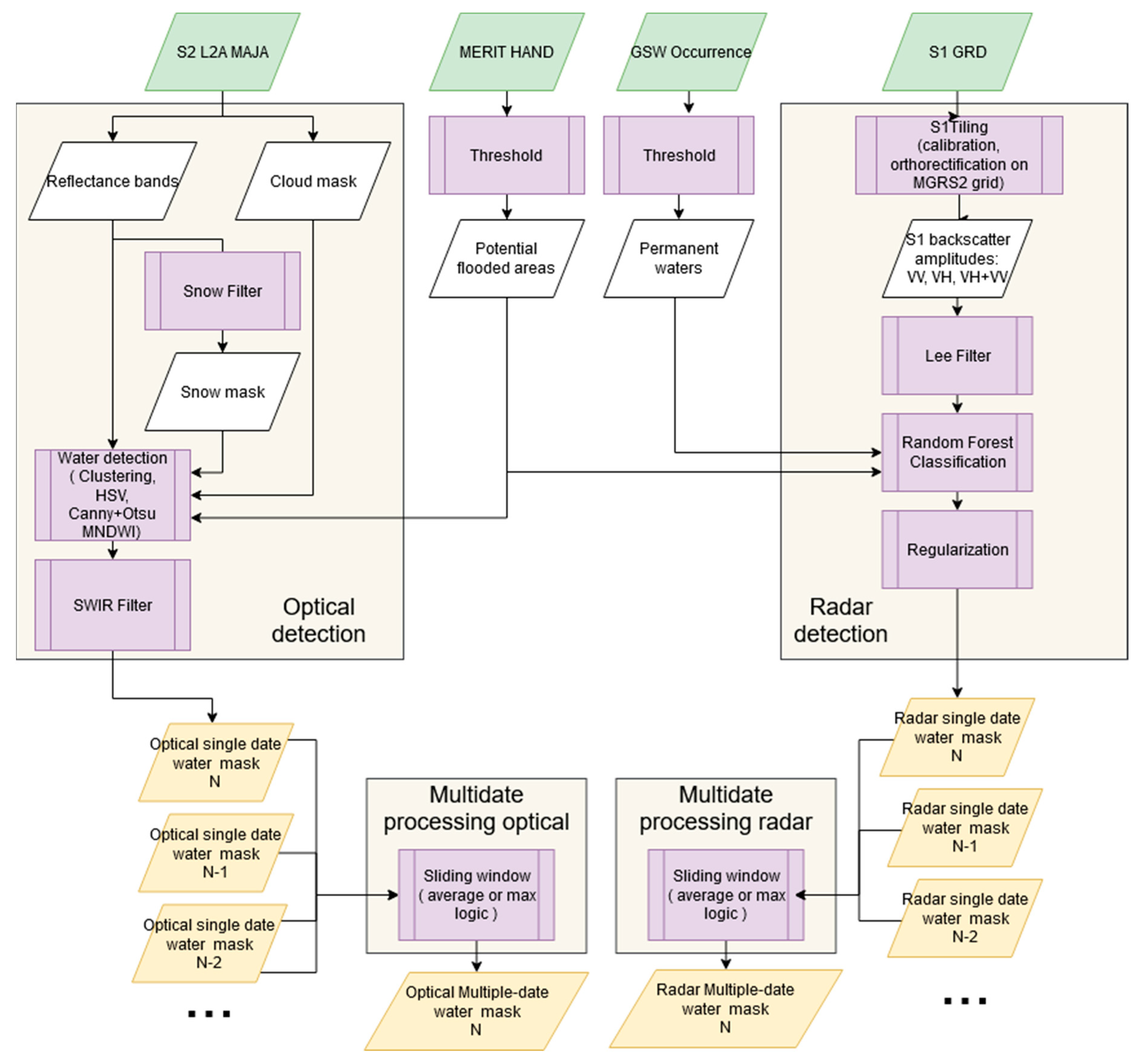
2.2. Water Detection Methods

The process to generate water masks is divided into two different fluxes for radar and optical images. Since Sentinel-1 and Sentinel-2 have similar resolutions, intermediary and output data are generated on the same grid (Military Grid Reference System-MGRS) and resolution, which facilitates comparing the results. For this work, all data are resampled at 10 m resolution. The following Figure 1 depicts the workflow for the water masks generation, which includes the multiple-date processing of single-date water masks.
On the optical part, optical reflectances and cloud/shadow masks are retrieved from the S2L2A MAJA product. Cloud/cloud-shadow/relief-shadow masks are interpreted as a “No Data” layer. Second, a snow filter is used. Some of the water detectors that are evaluated in this work use the Modified Normalized Difference Water Index (MNDWI), which has the same spectral definition as the Normalized Difference Snow Index (NDSI) [62], quite sensible for snow detection. Therefore, it is important to separate snowy regions first, before classifying water regions. Since MAJA snow masks have 240 m resolution, a finer snow detector has been developed for this study. To avoid commission errors with turbid waters, a new snow filter is proposed based on reflectance values: Red > 1200, Blue > 1500, Red/Blue < 1.5. This filter is based on the fact that many turbid waters are prone to red values and shadowed snow regions prone to bluish tones.
To limit commission errors on mountain ridges or shadowed zones in steep valley regions, the MERIT HAND product is used to identify only floodable zones. In our case, regions placed higher than 25 m above their direct drainage zone are not likely to be flooded and they are excluded from the water detection process. This level has been calculated by comparing GSW maximum extent with the resulting floodable area from HAND.
Concerning the optical water detection algorithms, three state of the art classifiers have been integrated for the evaluation: (1) Edge filter Canny and Otsu thresholding on MNDWI [9]; (2) Binary clustering on Hue/Saturation/Value dimensions issued from “PyIntertidalDEM” algorithm [63]; (3) Agglomerative Clustering issued from “WaterDetect” algorithm [25] in three variants: using two channels (SWIR band, NDWI), using three channels (SWIR band, NDWI, MNDWI) and using four channels (SWIR band, NDWI, MNDWI, MBWI [64]). Lastly, a SWIR filter is placed after the water detection classifiers based on values lower than 800.
The radar detection module first projects the input Sentinel-1 data to the Sentinel-2 grid, in order to work in equivalent layers. This process is handled by the S1Tiling chain [65], which does the calibration, projection, and concatenation of images in the MGRS2 grid. Multitemporal speckle filtering has not been applied, but a Lee filter applied on single date images is more appropriate as it accounts for edges. Multiple window sizes have been evaluated. On radar detection, a supervised method has been implemented based on Random Forest (100 estimators, max depth = 3, test size = 20%). Global Surface Water occurrence map is used as training data, where 2000 water samples (pixels) are obtained from permanent waters (occurrence > 90%) and 10,000 land samples from areas where water has been never detected (occurrence = 0%). Finally, a regularization process is done, to remove isolated “as water detected” pixels, through the “ClassificationMapRegularization’’ application from OrpheoToolBox [66], evaluated at different window sizes, and a single-date water mask is obtained.
Every optical and radar observation runs a water detection process to obtain a single-date water mask. Then, single-date water masks are combined together with a multiple-date process for a time-window/sampling period. Five time-windows were tested in this study: 5, 10, 15, 20, and 30 days. Two multiple-date merging methods have been developed. The “Average” method classifies a pixel of the mask as water if at least 50% of the observations were classified as water by the single date classifiers. The “Max” method classifies a pixel of the mask as water if it has been classified as water at least once by the single date classifiers. This last method is equivalent to the maximum surface water extent as observed during the time-window period by Sentinel-1&2.

2.3. Region of Interest Extraction Process and Surface Water Area Estimation

A geographical layer of water bodies area extent found within the studied MGRS2 tiles is created from an Optical Water Occurrence mask (OWO). The OWO is computed for each Sentinel-2 pixel as the ratio between the number of water detection over the number of valid observations for optical data. The water bodies area extent is built from the dilation by 50 m of the OWO exceeding 15%. Every targeted water body, localized by its coordinates, is associated with the closest water body area extent. The water area extent of a water body for a single date or a time-window water mask is computed as the sum of water pixels’ area extent (10 × 10 m) contained in this area.

2.4. Reference Data-Large Scenes Water Masks

In order to validate water masks for large scenes in different seasons, a reference dataset has been developed using Active Learning for Cloud Detection (ALCD) software exploiting Sentinel-2 images. The motivation behind the use of ALCD for validating results rather than a hydrological database comes from the fact that water bodies are highly subject to change in time, depending on the season, meteorological conditions, management policies, etc.
The ALCD software was developed initially to generate reference cloud masks which may be used to validate Sentinel-2 cloud masks, such as those generated operationally by MAJA. This approach has been applied to generate reference water masks based on Sentinel-2 L1C [67] imagery.
The reference water masks are generated using an iterative active learning procedure which enables the creation of an accurate reference mask in less than 3–5 h for a 110 × 110 km scene. For this, it is necessary to manually create reference points on the image, train the model (based on Random Forest of OTB [66]) and predict with ALCD, then add new reference points for the most problematic areas, repeat training/predictions cycles as many times as necessary (usually 5–7 iterations). The final step consists of a manual correction of persisting errors. For the training process, the following Sentinel-2 bands were used, B2: Blue, B3: Green, B4: Red, B8: NIR, B11: SWIR1, B12: SWIR2. In addition, derived indices such as MNDWI and slope information derived from SRTM [68] were also exploited.
The generated validation dataset has been shared in the ZENODO platform in open access [69]. A total of 14 sites have been covered on different eco-climatic zones (oceanic, Mediterranean, mountainous, continental) that are presented in Figure 2. Then, 26 scenes have been completely labelled on these sites on different seasons and conditions (snow, flood event, turbid waters, wetlands, urban areas, dry scenes), as described in Table 1.
Since the aim is to evaluate inland waters, coastal waters have been excluded using the GSHHG world shorelines database [70], applying a dilation of 400 m towards the land. The total surface of labelled data is 238,126 km2.
Concerning ALCD scenes accuracy, ALCD scenes have been evaluated over three parts of France covering heterogeneous water bodies. In the Ardeche region (Tile 31TFL), these results have been compared to a detailed static water database issued from watershed managers (3-Rivières watershed). In the Normandy (Tile 30UYV) and the Sologne regions (Tile 31TDV), the results have been compared to the TOPAGE static water database [71]. In each case, the size of un-detected water bodies was checked with their size distribution being around 85%, 10%, and 1% respectively for 0–0.1 ha, 0.1–0.2 ha, and 0.2–0.5 ha classes. Another result is that more than 90% of the water bodies larger than 0.5 ha were correctly detected. Accordingly, it is estimated that the water bodies above 0.5 ha are also similarly well detected over the other ALCD tiles.

2.5. Reference Data-Reservoirs Area

Time Series of in situ daily observations of 29 reservoirs in the Occitanie region, in the south of France, has been gathered to qualify area monitoring from 2017 to 2019. Given the water surface elevation Z(t) and volume V(t) series provided by reservoir managers, which contains bathymetric information on their relationship, the area S(t) time series has been calculated as follows. First, the derivative values of V(Z) function of each reservoir are calculated, resulting in S(Z). Hence, S(Z) is used to transform Z(t) time series to S(t) time series. Assuming Z(t) uncertainty of ±2 cm on in-situ measurements as a worst-case scenario during high filling rate periods, mean S(t) uncertainty has been computed as ±0.14 hectares or ±0.12% of the area in our reservoirs dataset. Such worst-case uncertainty is small compared to S(t) errors obtained from satellite estimations (see Section 3.2.3). As shown in Figure 3, the reference reservoir maximum sizes were distributed from 1200 ha to 38 ha. The geographical distribution of the reference reservoirs in the south of France may be also noticed in Figure 3.
To have a better understanding of the impact of the reservoirs’ state on the area estimations, all the measurements have been associated with a reservoir state: high filling rate (area of reservoir >80% quantile of the in-situ area time series), low filling rate (area of reservoir <20% quantile of the in-situ area time series), increasing filling rate (if the area is greater than the previous day and outside high/low range), decreasing filling rate (if the area is lower than the previous day and outside high/low range).

2.6. Large Scene Water Masks Assessment

The assessment of large scene water masks has been developed in two stages.
First, optical and radar classifiers have been evaluated on a single-date basis. This assessment included the estimation of the following indicators: accuracy, F1-score, precision, and recall. As well, we give the number of comparisons with F1-score lower than 0.5 shown as “failures’’, to provide an insight into the instability of the water detection method.
Second, the best optical and radar classifiers from the first stage have been selected based on their median F1-Score. Then, different multiple-date methods have been assessed based on the same indicators of the first stage.

2.7. Reservoirs Area Assessment

Since reference reservoirs have a wide range of maximum water surface areas (from 20 ha to 1200 ha), error metrics chosen for this study should consider reservoirs’ size disparity. Thus, error metrics based on relative and absolute relative error have been used for this assessment, using the following definitions:
r e l a t i v e   e r r o r = X X r e f X r e f
a b s o l u t e   o f   r e l a t i v e   e r r o r = a b s ( X X r e f X r e f )
where X is the reservoir area measured by satellite at a given date and Xref refers to the reservoir area obtained by in-situ measurements.

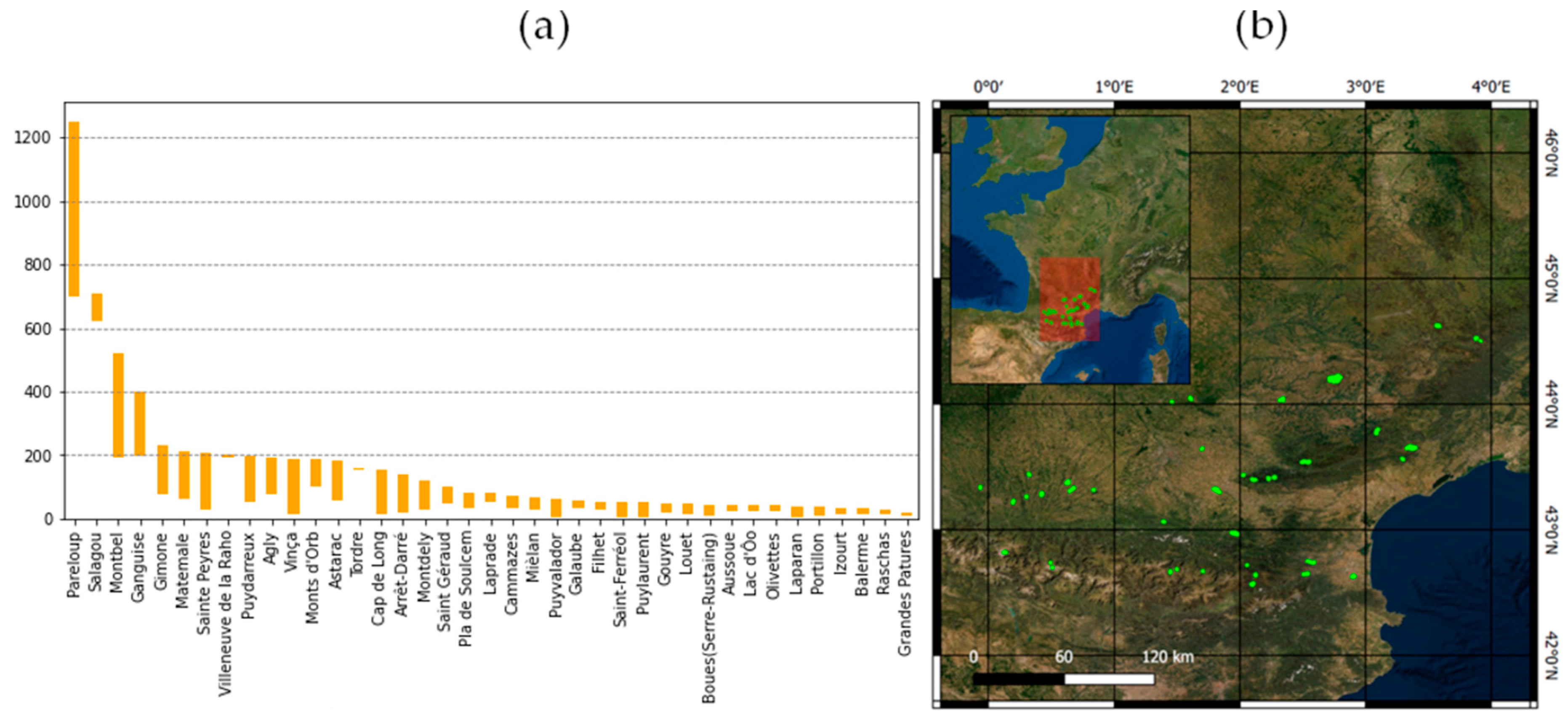
2.8. Reservoir Characteristics and Geomorphological Indicators

Reservoir characteristics might be also related to the quality of area monitoring. In this study, we propose to compare maximum area extent, altitude, and four geomorphological indexes to their results on Absolute Relative Error on area estimation.
The two first geomorphological indexes are the “Eroded Area” index, defined as the eroded surface area (maximum extent surface buffered by 50 m) divided by the maximum surface area, and the “Eroded Perimeter” index, which uses perimeter instead of area. Both indexes penalize reservoirs with narrow arms (widths <100 m will disappear), and yield higher values for large surfaces, where the loss of eroded surface is relatively lower compared to the maximum surface.
The second two morphological operations are the “Convex-Hull Area” index and the “Convex-Hull Perimeter” which use the Convex-Hull shape instead of the Eroded one. Low Convex-Hull Area or Perimeter index denotes a complex shape with sinuous boundaries.
Figure 4 shows examples of Maximum surface, Convex-Hull surface, and Eroded surface and their geomorphological values on four different reservoirs. Table 2 present the values of the proposed geomorphological indexes, where maximum values are represented with bold style.

3. Results

The proposed water detection methods and the multi-temporal approaches have been evaluated by two different assessment procedures. The first part addresses the quality of large scene water masks by comparing the resulting water maps to reference masks for specific dates. The second part addresses the quality assessment of area estimations for individual water bodies using in-situ data from 29 dams (two years’ time series). For both sections, single-date and multiple-date water detection results are compared separately for the optical and radar observations.

3.1. Large Scene Water Masks Evaluation

Every ground truth mask generated with ALCD has been compared with all the optical and radar water maps available in the range [D − 5, D + 5 days], where “D” is the acquisition date of the ALCD input mask. Radar and optical water detection methods have been evaluated independently. Optical input images with partial (cloudy) observations have been included in the evaluation; nevertheless, the areas marked as “cloud” or “shadow” on the S2-L2A input products are excluded from the evaluation. Thus, the intersection of all valid pixels from ground truth and classifier outputs are included in the evaluation (no sampling).

3.1.1. Optical Water Masks Evaluation at Single-Date Observation

Three different algorithms have been evaluated for water detection on Sentinel-2-L2A images: (1) Edge filter Canny and Otsu thresholding on MNDWI; (2) Binary clustering on Hue/Saturation/Value dimensions extracted from PyIntertidalDEM algorithm; (3) Agglomerative clustering based on the “WaterDetect” algorithm in three variants: two features (SWIR band, NDWI), three features (two first features + MNDWI) and using four features (three first features + MBWI). Furthermore, an additional filter has been evaluated on top of the basic algorithms: a threshold filter at 0.8 on the SWIR band. A total of 74 images have been evaluated and compared to the 26 ALCD ground truth masks using indicators described in Section 2.6. Results are presented in Table 3:
Agglomerative clustering methods (“Clustering”) achieved the best F1 median results over the 74 comparisons, providing the best scores on recall. Also, the “Clustering 3 channels” method with SWIR filter provided the best median F1 Score and the lowest number of failed detections (three images of F1 < 0.5 over 74 comparisons). The rest of the optical methods (Canny-Otsu MNDWI and HSV) have better Precision than Recall scores. SWIR filter has shown an improvement of median precision scores or number of failures at this evaluation.

3.1.2. Radar Water Masks Evaluation at Single-Date Observation

The radar water detection method, based on Random Forest trained on historic optical water detections, has been assessed through combinations of different window sizes of Lee speckle filters (unit: 10 m pixels) and output regularization filters based on ball structure (radius unit: 10 m pixels). A total of 123 images have been evaluated and compared to the 26 ALCD ground truth masks providing the following results, presented in Table 4:
The effect of larger preprocessing Lee filtering windows slightly improves the median recall score in detriment of a higher number of failures. The effect of a larger Regularisation window improves the median precision and the number of failed scenes. Regularisation has a cleaning effect on small, isolated detections or water omissions, produced by speckle and surface roughness irregularities present in crop bare soils or windy water surfaces.

3.1.3. Multiple-Date Water Masks Evaluation

The multiple-date water masks assessment considers different time window lengths and different methods to process single-date water masks.
The selected optical water detection algorithm, based on the best F1-score, is the “Clustering 3 channels” with a SWIR filter; the selected radar water detection algorithm is based on Random Forest with a regularisation size equal to two. Like in previous assessments, 74 optical evaluations and 104 radar evaluations have been performed. Results are shown on Table 5 their median values and number of failures:
Regarding radar results, “average” methods improve precision, and hence, F1-Score with longer time-windows. Recall remains constant even with increasing time-window length, whereas failures drop considerably if a time window is set. “Max” methods, on the contrary, worsen the performance when increasing the length of the time-window in precision and number of failures.
About optical results, “average” multiple-date methods do not improve scores for the general scene evaluation, and failures are increased. On the other hand, “Max” multiple-date methods decrease performance for longer windows.

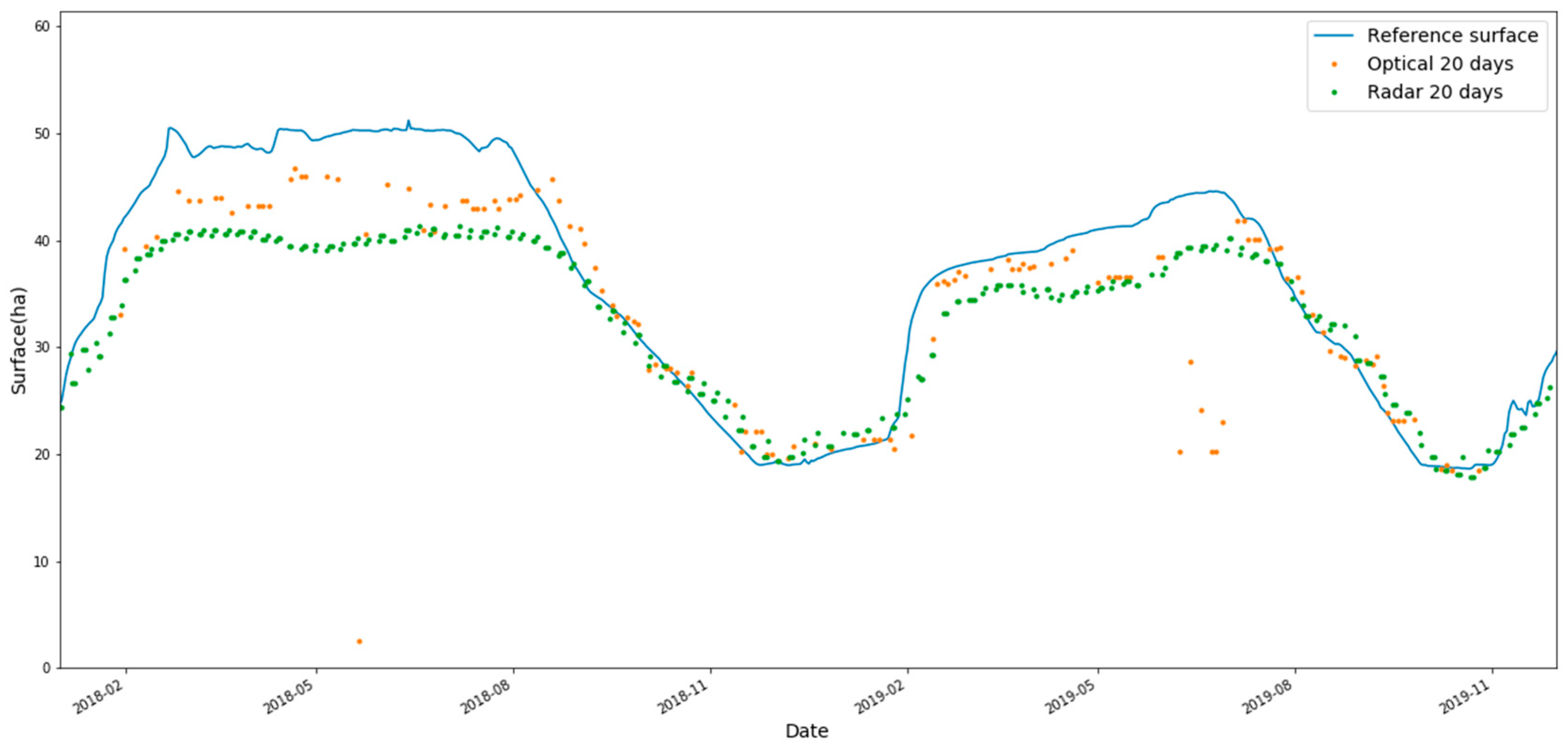
3.2. Area Monitoring Evaluation on Reservoirs

This evaluation is based on the comparison of reservoirs’ areas issued from satellite observations with daily in-situ measurements from 29 reservoirs in the South of France. Time series of two years (2018, 2019) have been used for this analysis. Figure 5 shows an example of reference area time-series and satellite area estimations for one reservoir.

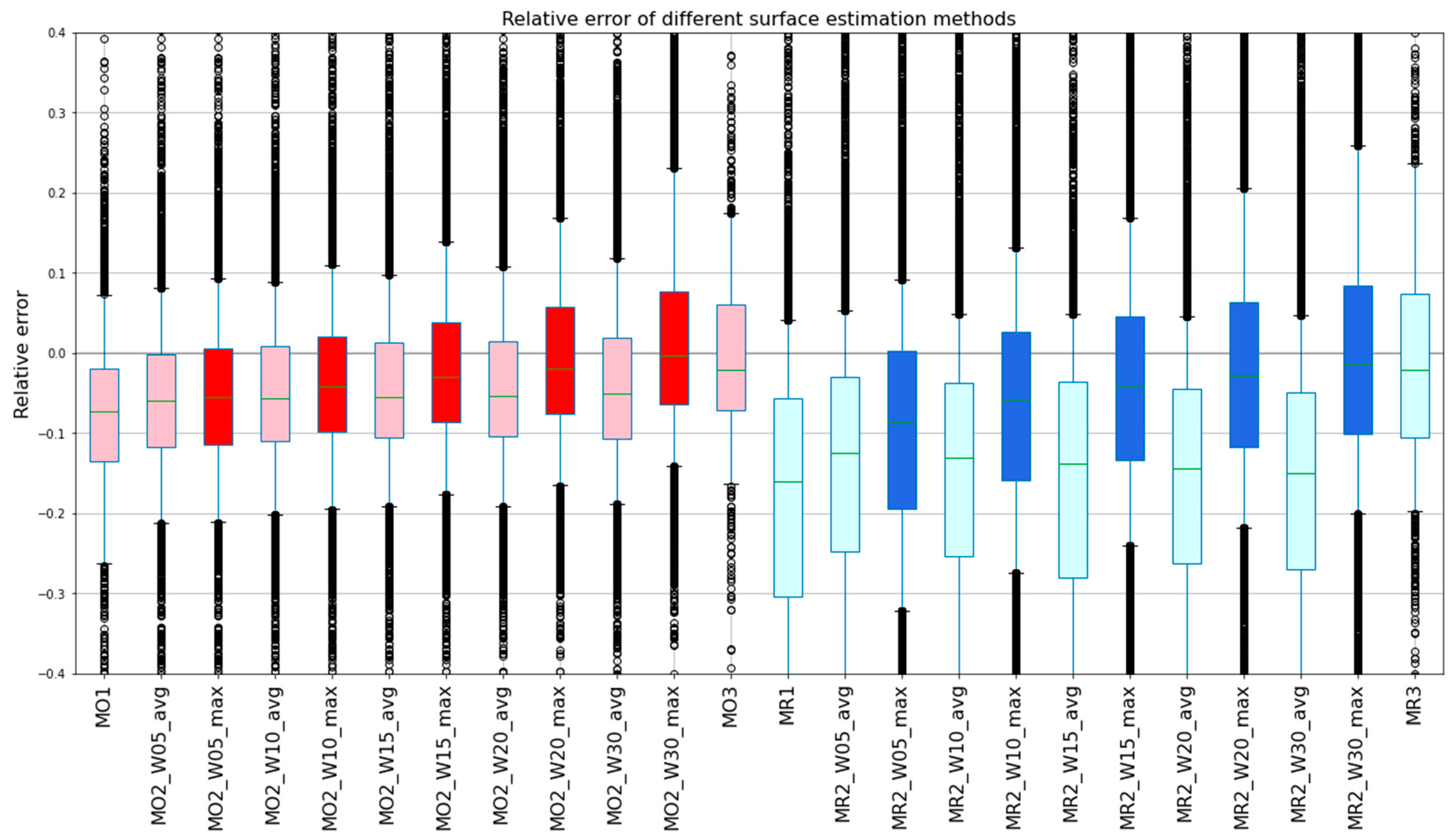
3.2.1. Error Assessment of Reservoirs Area Monitoring

The surface area of each water body is computed from a large-scene water mask, as described in Section 2.3, and error metrics are then processed, described in Section 2.7. The proposed reservoir monitoring methods are classified according to how large-scene water masks are generated using the following criteria:
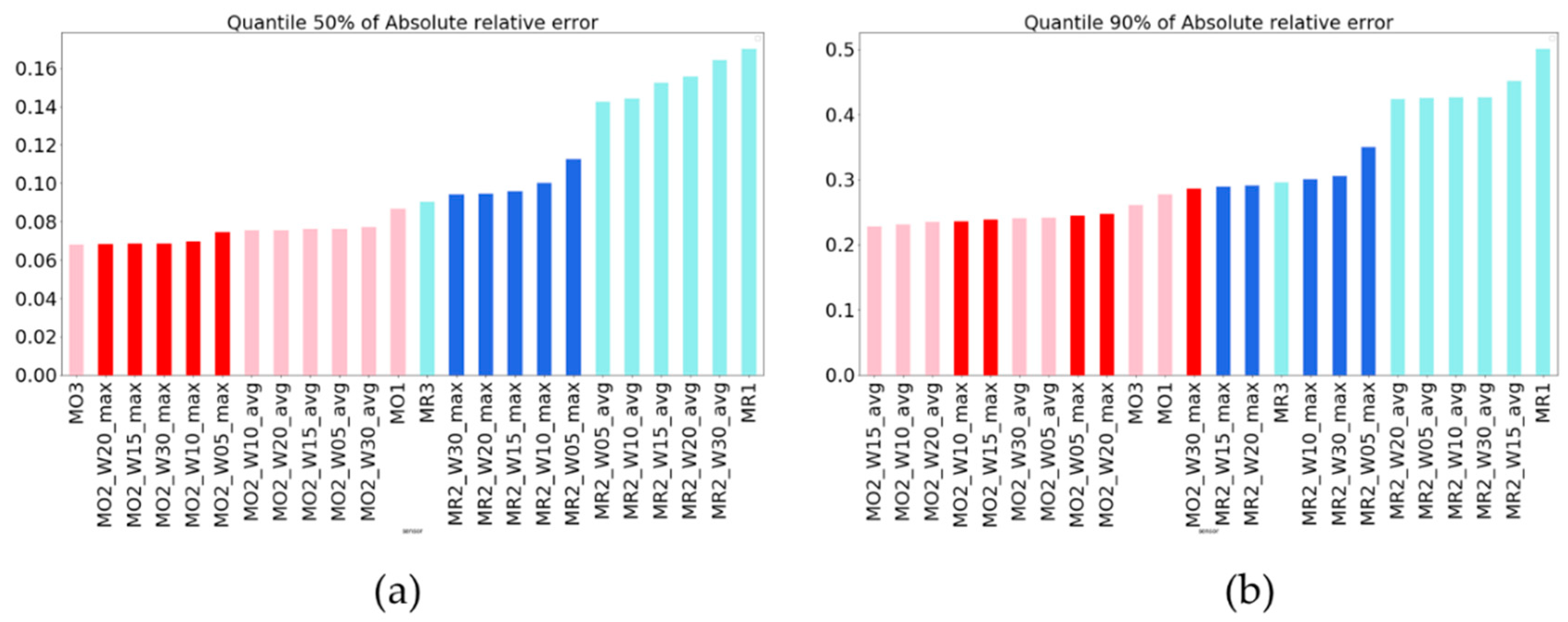
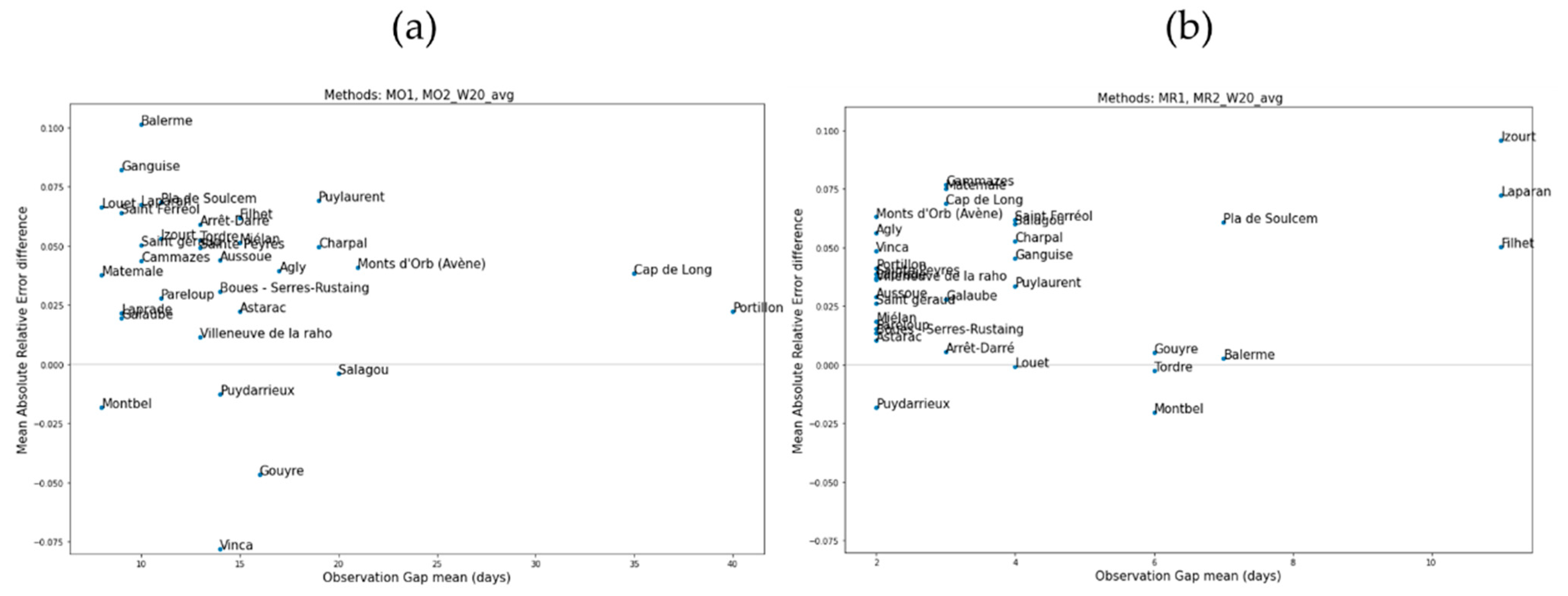
  • Sensor: optical measurements (“MO”) and radar measurements (“MR”), based on the same water classification methods evaluated in Section 3.1.3.
  • Single/Multi-date method: They are categorized in three classes: Single-date methods are based on just one satellite observation (“MO1”, “MR1”), multiple-date methods apply a backwards time-window (“MO2”, “MR2”) and the last methods calculate the sum of all the surfaces detected as water at least once during a natural month (“MO3”, “MR3”). Multiple-date methods (“MO2”, “MR2”) present two possible logics: average (“_avg”) and maximum pixel wise surface (“_max”), as described in Section 2.2. Also, multiple-date methods with time-windows have a suffix (“_WN”), where N is the time-window size in days.
In order to understand the general behavior of each method, all measurements for 29 reservoirs for two years are shown in Figure 6 by boxplots. Optical methods have been represented in red tone boxes and radar methods in blue tone boxes. Multiple-date methods based on “maximum” logic are represented with more intense colors. Green horizontal lines inside the boxes show median values. The box is bounded at 25% and 75% quantiles and whiskers are set on 10% and 90% quantiles.
Regarding median values for this global visualization, it may be noticed that all the methods have a generalized negative bias on reservoir area estimation. The optical method’s underestimations are less accused than the corresponding radar methods. For example, MO2_W15_avg has a median value of −5.49%, while the radar version MR2_W15_avg has a median value of −13.8%. Regarding the effect of time-windows, it may be observed that longer windows are associated with a reduced underestimation. For instance, median values on the optical values improve from −7.23% in MO1 to −5.28% in MO2_W20_avg. Radar median values improve from −16.04% in MR1 to −4.1% in MR2_W20_max. Among the time-window methods, those applying the “maximum” multi-date logic have smaller bias values than the equivalent “average” methods for the same window length. MO3 and MR3 methods may be considered equivalent to MO2_W30_max or MR2_W30_max methods where estimations are produced only once per month (only natural month data are considered). Their error boxplots are quite similar as expected. Respecting median values, MO2_W30_max and MR2_W30_max achieve better accuracies, with 0.3% and 1.3% respectively.

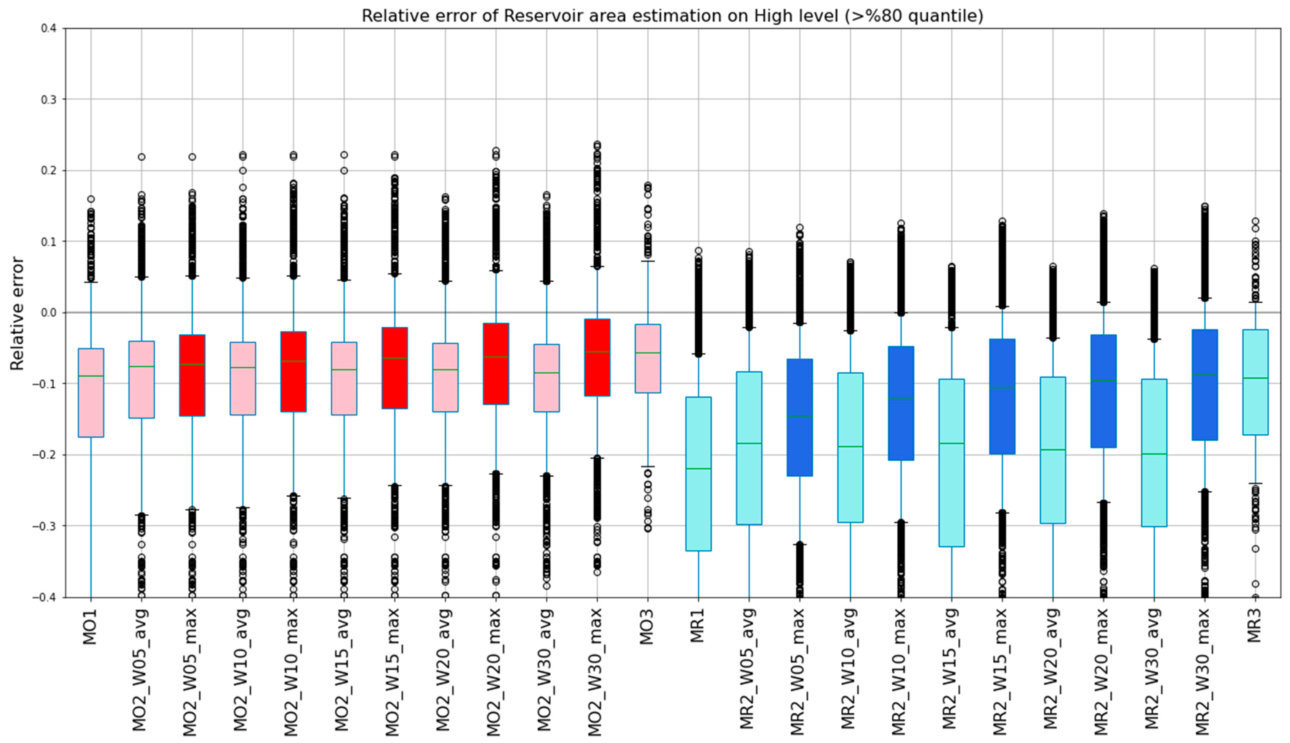
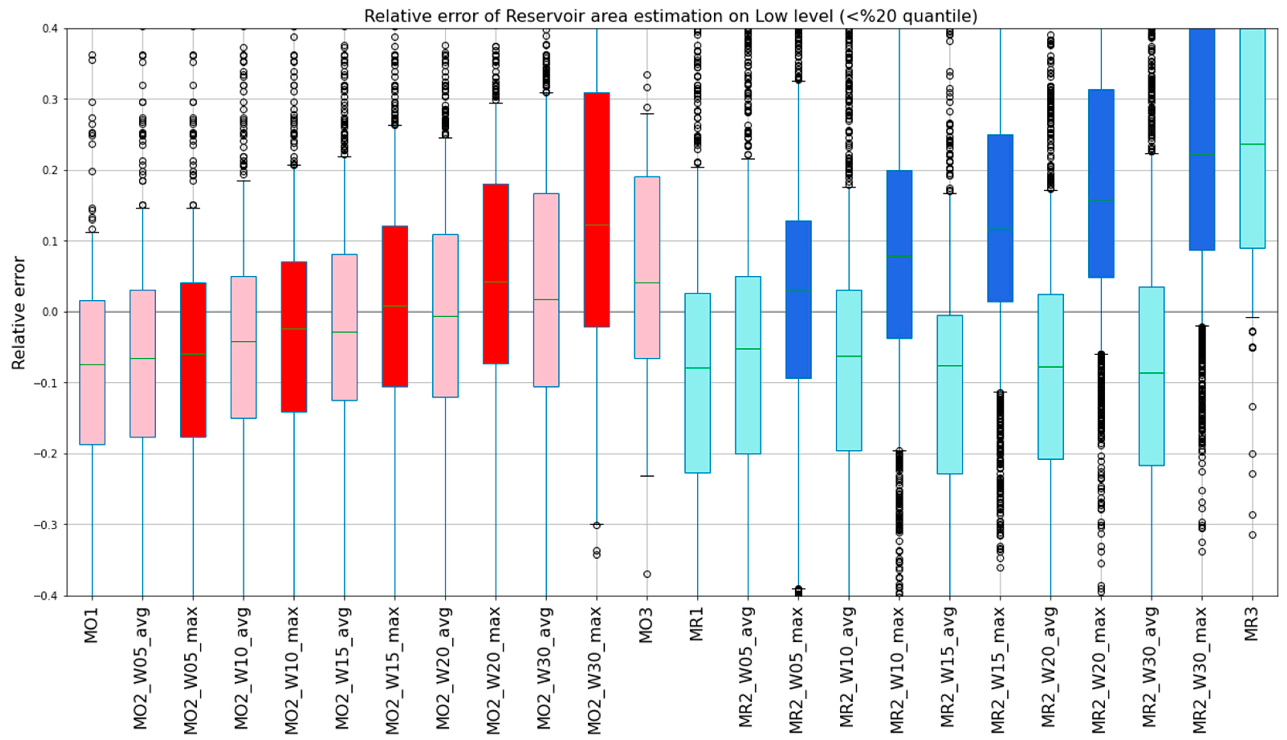
3.2.2. Influence of Reservoir Filling Rate

The dynamics of water stored in reservoirs have an impact on the water surface characteristics (area, nature of boundary water/land areas) and thus may affect the water mask quality for each reservoir. We define two contrasted hydrological conditions by subset the water area extent: high filling rate and low filling rate (see Section 2.5)
Figure 7 shows the same relative error of each method presented in Figure 6 but restricted to dates with high filling rate status. Two main differences appear. First, the general negative bias of area estimations is higher than in the global case. For example, median relative errors of “MO_W20_avg” change from −5.33% in all reservoirs status to −7.96% in the high filling rate. Second, this negative bias decreases less while increasing the time-window compared to the global case.
This generalised underestimation of the area extent detected for high filling rate periods might be explained by the dense vegetation often covering the rarely flooded shores and upstream parts of the reservoirs. Water detection algorithms are very affected in areas with dense vegetation in optical images [17] and SAR [72], as shown in Figure 8. Shrubs and small trees also affect radar detection, to a larger extent than optical data detection, as shown in water occurrence maps in Section 4.1. Confusions between sand and water are also a source of detection failures with radar data, as shown in the inner part of the lake in Figure 8.
The same analysis made for low filling rate periods shows different behaviors, as shown in Figure 9. In hydrologically drier conditions, bias increases with increasing time window. Time-window methods using “maximum” logic turn negative bias into high positive bias. The “average” method over 20 days leads to removing the negative bias observed with the optical data detection methods whereas radar detection biases are not improved with time window. This overestimation is mainly due to the integration of higher water level observations within the time window.

3.2.3. Analysis of Absolute of Relative Error on Reservoir Area Estimation

To provide a more comprehensive study on reservoir area estimation error and its dispersion, we propose to analyze absolute values of relative area errors from all the reservoir area estimations altogether. Working with absolute values, median or quantile error values better reflect all kinds of error, positive and negative. In Figure 10, we have sorted the quantile values (50%, 90%) of absolute of relative error of area estimation of each method for all reservoirs as a whole, and the following results may be observed:
  • On the optical methods, MO3 (maximum on natural month) provides the best results on quantile 50% (median value), but it performs worse on quantile 90% compared with other optical methods. Time-window methods based on “maximum” logic perform well on 50% quantiles, but they are not the best on 90%. Time-window methods based on “average” logic with 10-15-20 days perform well on quantile 90%. For example, the mean absolute relative error in MO1 is 16.9%, whereas MO2_W15_avg is 12.9%. In conclusion, “average” and “max” time-windows have similar positive results compared to single-date methods.
  • On the radar methods, MR3 (maximum on natural month) provides the best performance on both quantiles 50% and 90%; on the time-window methods, methods based on “maximum” outperform the “average” methods for both quantiles. For example, the mean absolute relative error in MR1 is 22.7%, whereas MR2_W10_avg is 19.5% and MR2_W10_max is 15.1%. For “maximum” methods, relatively long windows (20, 30 days) perform better than short windows (5, 10 days). For “average” methods, quantiles 50% are better with short windows (5, 10 days) but quantiles 90% are better with middle (10, 20 days) windows.
  • Any multi-temporal method (“MO2”, “MO3”, “MR2”, “MR3”) outperforms the other methods based on single observations (“MO1”, “MR1”) on quantile 50% and 90% of absolute of relative error on the area estimation.
  • Any optical method (“MO”) outperforms the other methods based on radar observations (“MR”) on quantile 50% and 90% of absolute of relative error on the area estimation.

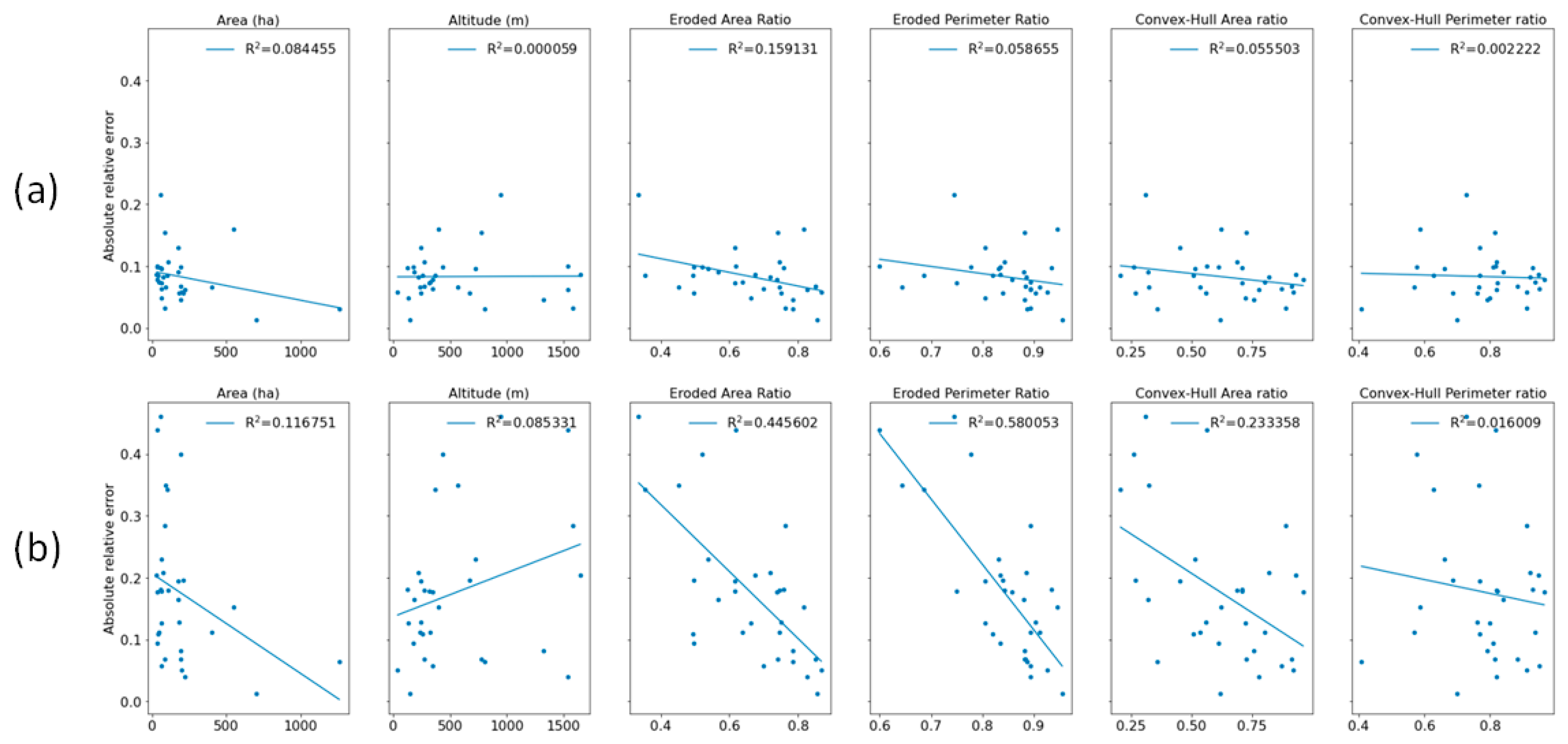
3.2.4. Geomorphological Influence on Area Estimation Quality

To have a better understanding, an analysis of optical and radar area monitoring error (median error) has been plotted against the maximum area, altitude, and four geomorphological indicators of all reservoirs in Figure 11. Separately for optical and radar methods, a linear regression function has been fitted for each ensemble of Area Monitoring Error and geomorphological information of each reservoir. For the optical method (MO2_W20_avg), individual geomorphological indicators show a poor correlation with area monitoring quality, with R2 values < 0.2. Using all morphological indices in one single linear model for optical, it yields a 0.42 R2 score, which is low. For Radar Methods (MR2_W20_avg), Eroded Perimeter and Area indexes have the most relevant information to predict the area monitoring quality, with R2 scores of 0.44 and 0.58. Results corroborate the idea that radar water detection is limited for narrow water areas (width <100 m) by the lower spatial resolution and the effect of bright adjacent land zones comparatively to Sentinel-2. This impacts significantly the total area extent detection accuracy. Using all morphological indices in one single linear model for radar yields a 0.67 R2 value. Hence, the presented geomorphological indices would better predict the quality of area estimation of each reservoir on radar methods than in optical ones. With respect to a maximum surface dataset of 104 reservoirs in the Occitanie region, we appreciate that 37.5% of reservoirs have Eroded Perimeter index values under 0.8, which suggests that they will have bad area estimation quality using radar methods (median absolute of relative error higher than 20%).

4. Discussion

4.1. Multitemporal Impact on Optical and Radar Detections

We presented a methodology to generate large-scale water maps and process them to monitor reservoir areas. In comparison with other works on reservoir monitoring based on optical surface observations [73,74] or radar observations [75], the presented surface and area estimation method proposes a multi-temporal approach. This strategy of merging multiple date information corrects occasional noisy events, acting as a temporal (not to confuse with spatial filter) low-pass filter on the time series. On the other hand, detection of rapid changes will be penalized, which affects reservoir area estimation (e.g., coastal reservoirs that change with the tide). Regarding end-to-end performance on reservoir area monitoring presented in Section 3.2.3, results show a general positive effect of multi-temporal approach on reservoir area estimation, for both radar and optical methods and for any kind of merging logic (average, max). Nevertheless, there are differences between radar and optical performances.
First, there are constant factors affecting water mask quality which are different for optical and radar observations. On SAR images from Sentinel-1, water detection is based on spotting zones with low backscattering. When a water body is contiguous to high radar reflectance elements (trees, artificial structures as bridges, or walls), the SAR impulse response of these bright elements affects the adjacent low signal zones on water surfaces. Being Sentinel-1 resolution equal to 20 × 22 m and affecting at least one adjacent pixel, it may represent a loss of 40 m when measuring river widths, or erosion of 20 m inside the perimeter of a lake or reservoir. Detection problems by trees are aggravated by Sentinel-1 high incidence angle range (29.1°–46°) compared to Sentinel-2 (0°–10.1°). There are other constant factors that challenge the radar water detection at boundaries, such as sand, which may have very low backscatter for certain angles and certain moisture levels [44], or the effect of vegetation at the surface water. Other relatively constant factors (which duration is longer than several weeks) also affect optical detection, like a tree or urban shadows [76] or sunglint [77]. As a result, water boundaries zones with sand and vegetation are often better detected with optical measurements. Figure 8 and Figure 12 show the systematic drastic drop of radar occurrence near water bodies shores, especially for forested surroundings. On the contrary, optical occurrence remains stable and drops closer to the shore.
Second, the quality of the masks is affected by variable observation conditions depending on the method (optical, radar). The multi-temporal approach allows to correct and erase false detections inside the time-window: clouds or cloud shadows perturbations for optical detection; speckle, certain bare soil conditions (roughness, soil moisture), and water roughness variations due to wind for radar detection [78]. In this study, clouds or cloud shadows are generally flagged and removed by the MAJA preprocessing chain. Some remaining artifacts (cloud or shadow not detected) may sporadically affect detection quality. On the contrary, scene variable conditions that perturb the radar detection quality, such as speckle, water/soil roughness, or soil moisture, are always present in radar images and cannot be flagged. Hence, radar water masks quality might be more frequently affected by undetected changes of these variables.
Multiple-date methods statistically improve more unflagged radar detections than flagged optical detections. This should come to a reduction of omission errors in rough waters or commission errors in bare soils, and compensates for speckle effects in omission and commission, as illustrated in Figure 13. Also, multiple-date methods like maximum extent logic combine ascending and descending radar views of reservoirs surrounded by trees, reducing the shadowed area and improving area estimation. This is an important result for regions that have a permanent cloud coverage in tropical or polar areas, for which the Sentinel-1 data time-series could be more complete/accurate than cloud-free composite Sentinel-2.
Given the cited differences between optical and radar methods, which are affected by different constant and variable factors, we have kept a separate analysis for reservoir monitoring evaluation. In this context, it should be taken into account that water boundaries detection will be different on optical and radar sensors for thin water bodies (<50 m), sandy shores, artificial structures, and some vegetation types above water. Nevertheless, merging both outputs together is possible and complementary (better accuracies on optical methods and assured systematic radar observations). On complex zones like wetlands, the benefits of merging both sensor measurements have been already shown [79] or in flood duration analysis [74].

4.2. Observation Frequency

The presented work has been evaluated in metropolitan France, where Sentinel-1 and Sentinel-2 observation conditions might not be completely generalizable. Sentinel-1 observations are more frequent (2–6 days) than other zones in the world (12 days) [55,80]. Also, Sentinel-2 observations in tropical and arctic zones are very limited due to frequent clouds. With regard to our reference reservoirs, there is a notorious difference in frequency of reservoir observations due to swaths overlap or local climatological conditions for optical measurements. Figure 14 shows how time-window with average logic using 20 days changes the quality of the area estimations depending on the mean duration between clear observations. This effect is expressed as the difference of the mean absolute of relative error multiple date estimations (MO2_W20_avg, MR2_W20_avg) compared to single date observations (MO1, MR1). In view of the results, where the estimations are improved in general, it cannot be stated that more frequent clear observations increase accuracy for either optical or radar methods. In other words, even if the time-window captures a small number of observations, quality improvement on area estimation has been observed. This fact could justify longer time-windows in zones with less frequent Sentinel-1 observations, with durations like 12 or 24 days in order to include at least one or two observations.

5. Conclusions

We argued at the beginning of the article that multiple-date approaches had to be considered and evaluated for the improvement of water maps (large scenes) and the accuracy of reservoir area estimation. Through the evaluation of 26 reference water maps (110 km × 110 km at 10 m resolution), and the analysis of 29 reservoirs in France for 2 years, we have shown the improvement of accuracy for optical (Sentinel-2) and radar (Sentinel-1) measurements in two ways. First, large scene water maps scores have improved significantly on radar multi-date approaches (an increase of 0.08 in F-Score with average logic at 30 days), while optical maps just yield similar results to multiple-date. On the reservoir area assessment, both multiple dates approaches (average and maximum logics) improved results for both radar and optical approaches for any time-window length. For example, the mean absolute relative error on area estimation from single date radar measurements improved from 22% to 14% using the Maximum logic on 15 days. For optical data, even if large scene quality did not apparently improve (similar F1-score), the mean absolute of relative error on reservoir area estimation decreases from 16.9% to 12.9% using the Average logic on 15 days. Table 6 summarizes the impacts of multiple-date approach compared to single-date results.
Additionally, the present work yields a quality evaluation and comparison of radar and optical water maps, using state of the art methods. While similar in the precision score (0.9), optical water maps had better median recall scores (0.9) than radar (0.75), which may be explained by difficulties of radar on smaller water bodies like thin rivers or small ponds. Concerning reservoir area monitoring, optical estimations outperform radar. Optical approaches yield a median absolute of relative error of 6.8% (30 days with “maximum” logic) while radars yield 9.5% (30 days with maximum logic). It is important to remark that both methods have a tendency to underestimate area (negative bias), being more significant on the radar. Considering the water level status of reservoirs, our methods have shown better estimations at low filling rate conditions than at high filling rates. This observation is important for application purposes, as low filling rates occur during dry conditions when water restrictions and water shortage happens. Lastly, in order to predict the radar performance on reservoir area monitoring, we propose the analysis of the “Eroded Area Ratio”, showing a considerable correlation with area estimation quality (mean of absolute of relative error).
As a result of conducting this research, we propose two improvements to future water maps and reservoir monitoring systems based on satellite measurements. First, future water maps products should take advantage of multiple-date approaches to improve mapping accuracy, especially in radar observations. We propose to use time windows between 10–20 days applying “average” logic which yields significant improvements on large-scale water maps and reservoirs area estimation. In zones with less frequency of Sentinel-1 observations (mainly outside Europe), time-windows of 12–24 days would be recommended. Second, reservoir filling rate may influence the quality of area estimations, being critical on full reservoirs surrounded by dense vegetation or artificial structures affecting radar. Some solutions are proposed for future investigations: flag high-filled reservoir measurements surrounded by such conditions by means of land cover maps; reconstruct area dynamics just focusing in zones not surrounded by vegetation of artificial structures [75] or correct area dynamics using auxiliary measurements, such as altimetry, digital elevation models or in situ measurements. New altimetry systems providing a larger number of tracked water bodies in a global approach, like IceSat2 based on Lidar [81], altimeters Sentinel-3 [82], Sentinel-6 [83], and the future SWOT mission [84], will provide essential information to be combined with the proposed area estimations. Such a combination will help to better determine the volume dynamics of reservoirs and lakes globally. As a final idea and with regard to the results of this work, we suggest that operational reservoir monitoring systems should combine both sensors: optical measurements, with better accuracies, and radar measurements, with more observations independent from cloud conditions, to provide a complete as possible insight on water dynamics.

Author Contributions

Conceptualization: S.P.-L.; methodology, S.P.-L. and S.F.; software, S.P.-L., M.C.R.C.; validation, S.P.-L.; formal analysis, S.P.-L.; investigation, S.P.-L., S.F. and J.-M.M.; resources, S.P.-L.; data curation, S.P.-L., T.L. and J.M.; writing—original draft preparation, S.P.-L., S.F.; writing—review and editing, S.P.-L., S.F., M.C.R.C., J.-M.M., T.L. and J.M.; visualization, S.P.-L.; supervision, S.P.-L.; project administration, S.P.-L. All authors have read and agreed to the published version of the manuscript.

Funding

This research was funded by Supported by the French Future Investment Programme (Programme d’Investissment d’Avenir, PIA) through the SWOT Downstream program for hydrological applications and CNES agency.

Institutional Review Board Statement

Not applicable.

Informed Consent Statement

Not applicable.

Data Availability Statement

The data presented in this study are available on request from the corresponding author. The data are not publicly available due to privacy of the reservoirs reference data.

Acknowledgments

Reference data from French reservoirs have been collected by M.Blanc (Regional direction DREAL Occitanie, France) and processed by P.Kosuth (Ministry of Ecological Transition, France). Large-scene reference data has been enriched and curated by UNISTRA-Icube (J.Briant, M.Studer, H.Yesou) and C-S (G.Nicolas). Data processing and validation processes have been optimized by C-S (A.Bricier). The project relies heavily on open-source software. All programming was done in OTB 7.2, Python 3.7, and associated libraries, including Numpy, Pandas and Matplotlib.

Conflicts of Interest

The authors declare no conflict of interest. The funders had no role in the design of the study; in the collection, analyses, or interpretation of data; in the writing of the manuscript, or in the decision to publish the results.

References

  1. Biemans, H.; Haddeland, I.; Kabat, P.; Ludwig, F.; Hutjes, R.W.A.; Heinke, J.; Von Bloh, W.; Gerten, D. Impact of reservoirs on river discharge and irrigation water supply during the 20th century. Water Resour. Res. 2011, 47. [Google Scholar] [CrossRef] [Green Version]
  2. Zhou, T.; Nijssen, B.; Gao, H.; Lettenmaier, D.P. The Contribution of Reservoirs to Global Land Surface Water Storage Variations. J. Hydrometeorol. 2016, 17, 309–325. [Google Scholar] [CrossRef]
  3. Habets, F.; Molénat, J.; Carluer, N.; Douez, O.; Leenhardt, D. The cumulative impacts of small reservoirs on hydrology: A review. Sci. Total Environ. 2018, 643, 850–867. [Google Scholar] [CrossRef] [Green Version]
  4. Blanc, E.; Strobl, E. Is Small Better? A Comparison of the Effect of Large and Small Dams on Cropland Productivity in South Africa. World Bank Econ. Rev. 2013, 28, 545. Available online: https://ssrn.com/abstract=2309848 (accessed on 9 August 2021). [CrossRef] [Green Version]
  5. Acheampong, E.N.; Ozor, N.; Sekyi-Annan, E. Development of small dams and their impact on livelihoods: Cases from northern Ghana. Afr. J. Agric. Res. 2014, 9, 1867–1877. [Google Scholar] [CrossRef]
  6. Pekel, J.-F.; Cottam, A.; Gorelick, N.; Belward, A.S. High-resolution mapping of global surface water and its long-term changes. Nature 2016, 540, 418–422. [Google Scholar] [CrossRef]
  7. Busker, T.; De Roo, A.; Gelati, E.; Schwatke, C.; Adamovic, M.; Bisselink, B.; Pekel, J.-F.; Cottam, A. A global lake and reservoir volume analysis using a surface water dataset and satellite altimetry. Hydrol. Earth Syst. Sci. 2019, 23, 669–690. [Google Scholar] [CrossRef] [Green Version]
  8. McFeeters, S.K. The use of the Normalized Difference Water Index (NDWI) in the delineation of open water features. Int. J. Remote Sens. 1996, 17, 1425–1432. [Google Scholar] [CrossRef]
  9. Xu, H. Modification of normalised difference water index (NDWI) to enhance open water features in remotely sensed imagery. Int. J. Remote Sens. 2006, 27, 3025–3033. [Google Scholar] [CrossRef]
  10. Du, Y.; Zhang, Y.; Ling, F.; Wang, Q.; Li, W.; Li, X. Water Bodies’ Mapping from Sentinel-2 Imagery with Modified Normalized Difference Water Index at 10-m Spatial Resolution Produced by Sharpening the SWIR Band. Remote Sens. 2016, 8, 354. [Google Scholar] [CrossRef] [Green Version]
  11. Feyisa, G.L.; Meilby, H.; Fensholt, R.; Proud, S. Automated Water Extraction Index: A new technique for surface water mapping using Landsat imagery. Remote Sens. Environ. 2014, 140, 23–35. [Google Scholar] [CrossRef]
  12. Acharya, T.D.; Subedi, A.; Lee, D.H. Evaluation of Water Indices for Surface Water Extraction in a Landsat 8 Scene of Nepal. Sensors 2018, 18, 2580. [Google Scholar] [CrossRef] [PubMed] [Green Version]
  13. Fisher, A.; Flood, N.; Danaher, T. Comparing Landsat water index methods for automated water classification in eastern Australia. Remote Sens. Environ. 2016, 175, 167–182. [Google Scholar] [CrossRef]
  14. Yang, X.; Qin, Q.; Yésou, H.; Ledauphin, T.; Koehl, M.; Grussenmeyer, P.; Zhu, Z. Monthly estimation of the surface water extent in France at a 10-m resolution using Sentinel-2 data. Remote Sens. Environ. 2020, 244, 111803. [Google Scholar] [CrossRef]
  15. Otsu, N. A Threshold Selection Method from Gray-Level Histograms. IEEE Trans. Syst. Man Cybern. 1979, 9, 62–66. [Google Scholar] [CrossRef] [Green Version]
  16. Pekel, J.-F.; Vancutsem, C.; Bastin, L.; Clerici, M.; Vanbogaert, E.; Bartholomé, E.; Defourny, P. A near real-time water surface detection method based on HSV transformation of MODIS multi-spectral time series data. Remote Sens. Environ. 2014, 140, 704–716. [Google Scholar] [CrossRef] [Green Version]
  17. Pekel, J.F.; Belward, A.; Gorelick, N. Global Water Surface Dynamics: Toward a Near Real Time Monitoring Using Landsat and Sentinel Data. AGU Fall Meet. Abstr. 2017, 2017, GC11C-0742. [Google Scholar]
  18. Ngoc, D.D.; Loisel, H.; Jamet, C.; Vantrepotte, V.; Duforêt-Gaurier, L.; Minh, C.D.; Mangin, A. Coastal and inland water pixels extraction algorithm (WiPE) from spectral shape analysis and HSV transformation applied to Landsat 8 OLI and Sentinel-2 MSI. Remote Sens. Environ. 2019, 223, 208–228. [Google Scholar] [CrossRef]
  19. Doña, C.; Morant, D.; Picazo, A.; Rochera, C.; Sánchez, J.; Camacho, A. Estimation of Water Coverage in Permanent and Temporary Shallow Lakes and Wetlands by Combining Remote Sensing Techniques and Genetic Programming. Application to the Mediterranean Basin of the Iberian Peninsula. Remote Sens. 2021, 13, 652. [Google Scholar] [CrossRef]
  20. Hollstein, A.; Segl, K.; Guanter, L.; Brell, M.; Enesco, M. Ready-to-Use Methods for the Detection of Clouds, Cirrus, Snow, Shadow, Water and Clear Sky Pixels in Sentinel-2 MSI Images. Remote Sens. 2016, 8, 666. [Google Scholar] [CrossRef] [Green Version]
  21. Yousefi, P.; Jalab, H.A.; Ibrahim, R.W.; Noor, N.F.M.; Ayub, M.N.; Gani, A. Water-Body Segmentation in Satellite Imagery Applying Modified Kernel Kmeans. Malays. J. Comput. Sci. 2018, 31, 143–154. [Google Scholar] [CrossRef]
  22. Kaplan, G.; Avdan, U. Object-based water body extraction model using Sentinel-2 satellite imagery. Eur. J. Remote Sens. 2017, 50, 137–143. [Google Scholar] [CrossRef] [Green Version]
  23. Wieland, M.; Martinis, S. A Modular Processing Chain for Automated Flood Monitoring from Multi-Spectral Satellite Data. Remote Sens. 2019, 11, 2330. [Google Scholar] [CrossRef] [Green Version]
  24. Bangira, T.; Alfieri, S.M.; Menenti, M.; Van Niekerk, A. Comparing Thresholding with Machine Learning Classifiers for Mapping Complex Water. Remote Sens. 2019, 11, 1351. [Google Scholar] [CrossRef] [Green Version]
  25. Cordeiro, M.C.; Martinez, J.-M.; Peña-Luque, S. Automatic water detection from multidimensional hierarchical clustering for Sentinel-2 images and a comparison with Level 2A processors. Remote Sens. Environ. 2021, 253, 112209. [Google Scholar] [CrossRef]
  26. Main-Knorn, M.; Pflug, B.; Louis, J.; Debaecker, V.; Müller-Wilm, U.; Gascon, F. Sen2Cor for Sentinel. In Proceedings of the Image and Signal Processing for Remote Sensing XXIII, Warsaw, Poland, 11–13 September 2017; Volume 10427. [Google Scholar]
  27. Hagolle, O.; Huc, M.; Pascual, D.V.; Dedieu, G. A multi-temporal method for cloud detection, applied to FORMOSAT-2, VENµS, LANDSAT and SENTINEL-2 images. Remote Sens. Environ. 2010, 114, 1747–1755. [Google Scholar] [CrossRef] [Green Version]
  28. Liu, K.; Song, C.; Wang, J.; Ke, L.; Zhu, Y.; Zhu, J.; Ma, R.; Luo, Z. Remote Sensing-Based Modelling of the Bathymetry and Water Storage for Channel-Type Reservoirs Worldwide. Water Resour. Res. 2020, 56, 027147. [Google Scholar] [CrossRef]
  29. Evans, T.L.; Costa, M.; Telmer, K.; Silva, T. Using ALOS/PALSAR and RADARSAT-2 to Map Land Cover and Seasonal Inundation in the Brazilian Pantanal. IEEE J. Sel. Top. Appl. Earth Obs. Remote Sens. 2010, 3, 560–575. [Google Scholar] [CrossRef]
  30. Chapman, B.; McDonald, K.; Shimada, M.; Rosenqvist, A.; Schroeder, R.; Hess, L. Mapping Regional Inundation with Spaceborne L-Band SAR. Remote Sens. 2015, 7, 5440. [Google Scholar] [CrossRef] [Green Version]
  31. Brisco, B.; Short, N.; van der Sanden, J.J.; Landry, R.; Raymond, D. A semi-automated tool for surface water mapping with RADARSAT. Can. J. Remote Sens. 2009, 35, 336–344. [Google Scholar] [CrossRef]
  32. Matgen, P.; Hostache, R.; Schumann, G.; Pfister, L.; Hoffmann, L.; Savenije, H. Towards an automated SAR-based flood monitoring system: Lessons learned from two case studies. Phys. Chem. Earth Parts A/B/C 2011, 36, 241–252. [Google Scholar] [CrossRef]
  33. Pham-Duc, B.; Prigent, C.; Aires, F. Surface Water Monitoring within Cambodia and the Vietnamese Mekong Delta over a Year, with Sentinel-1 SAR Observations. Water 2017, 9, 366. [Google Scholar] [CrossRef] [Green Version]
  34. Clement, M.; Kilsby, C.; Moore, P. Multi-temporal synthetic aperture radar flood mapping using change detection. J. Flood Risk Manag. 2018, 11, 152–168. [Google Scholar] [CrossRef]
  35. Huang, W.; De Vries, B.; Huang, C.; Lang, M.W.; Jones, J.W.; Creed, I.F.; Carroll, M.L. Automated Extraction of Surface Water Extent from Sentinel-1 Data. Remote Sens. 2018, 10, 797. [Google Scholar] [CrossRef] [Green Version]
  36. Bolanos, S.; Stiff, D.; Brisco, B.; Pietroniro, A. Operational Surface Water Detection and Monitoring Using Radarsat. Remote Sens. 2016, 8, 285. [Google Scholar] [CrossRef] [Green Version]
  37. Hardy, A.; Ettritch, G.; Cross, D.E.; Bunting, P.; Liywalii, F.; Sakala, J.; Silumesii, A.; Singini, D.; Smith, M.; Willis, T.; et al. Automatic Detection of Open and Vegetated Water Bodies Using Sentinel 1 to Map African Malaria Vector Mosquito Breeding Habitats. Remote Sens. 2019, 11, 593. [Google Scholar] [CrossRef] [Green Version]
  38. Huth, J.; Gessner, U.; Klein, I.; Yesou, H.; Lai, X.; Oppelt, N.; Kuenzer, C. Analyzing Water Dynamics Based on Sentinel-1 Time Series—a Study for Dongting Lake Wetlands in China. Remote Sens. 2020, 12, 1761. [Google Scholar] [CrossRef]
  39. O’Grady, D.; Leblanc, M.; Gillieson, D. Use of ENVISAT ASAR Global Monitoring Mode to complement optical data in the mapping of rapid broad-scale flooding in Pakistan. Hydrol. Earth Syst. Sci. 2011, 15, 3475–3494. [Google Scholar] [CrossRef] [Green Version]
  40. Manjusree, P.; Kumar, L.; Bhatt, C.M.; Rao, G.S.; Bhanumurthy, V. Optimization of threshold ranges for rapid flood inundation mapping by evaluating backscatter profiles of high incidence angle SAR images. Int. J. Disaster Risk Sci. 2012, 3, 113–122. [Google Scholar] [CrossRef] [Green Version]
  41. White, L.; Brisco, B.; Pregitzer, M.; Tedford, B.; Boychuk, L. RADARSAT-2 Beam Mode Selection for Surface Water and Flooded Vegetation Mapping. Can. J. Remote Sens. 2014, 40, 135–151. [Google Scholar] [CrossRef]
  42. Li, J.; Wang, S. An automatic method for mapping inland surface waterbodies with Radarsat-2 imagery. Int. J. Remote Sens. 2015, 36, 1367–1384. [Google Scholar] [CrossRef]
  43. Martinis, S.; Twele, A.; Voigt, S. Unsupervised Extraction of Flood-Induced Backscatter Changes in SAR Data Using Markov Image Modeling on Irregular Graphs. IEEE Trans. Geosci. Remote Sens. 2011, 49, 251–263. [Google Scholar] [CrossRef]
  44. Martinis, S.; Plank, S.; Ćwik, K. The Use of Sentinel-1 Time-Series Data to Improve Flood Monitoring in Arid Areas. Remote Sens. 2018, 10, 583. [Google Scholar] [CrossRef] [Green Version]
  45. Bioresita, F.; Puissant, A.; Stumpf, A.; Malet, J.-P. A Method for Automatic and Rapid Mapping of Water Surfaces from Sentinel-1 Imagery. Remote Sens. 2018, 10, 217. [Google Scholar] [CrossRef] [Green Version]
  46. Chini, M.; Hostache, R.; Giustarini, L.; Matgen, P. A Hierarchical Split-Based Approach for Parametric Thresholding of SAR Images: Flood Inundation as a Test Case. IEEE Trans. Geosci. Remote Sens. 2017, 55, 6975–6988. [Google Scholar] [CrossRef]
  47. Senthilnath, J.; Shenoy, H.V.; Rajendra, R.; Omkar, S.N.; Mani, V.; Diwakar, P.G. Integration of speckle de-noising and image segmentation using Synthetic Aperture Radar image for flood extent extraction. J. Earth Syst. Sci. 2013, 122, 559–572. [Google Scholar] [CrossRef] [Green Version]
  48. Hornacek, M.; Wagner, W.; Sabel, D.; Truong, H.-L.; Snoeij, P.; Hahmann, T.; Diedrich, E.; Doubkova, M. Potential for High Resolution Systematic Global Surface Soil Moisture Retrieval via Change Detection Using Sentinel. IEEE J. Sel. Top. Appl. Earth Obs. Remote Sens. 2012, 5, 1303–1311. [Google Scholar] [CrossRef]
  49. Martinez, J.-M.; Le Toan, T. Mapping of flood dynamics and spatial distribution of vegetation in the Amazon floodplain using multitemporal SAR data. Remote Sens. Environ. 2007, 108, 209–223. [Google Scholar] [CrossRef]
  50. Twele, A.; Cao, W.; Plank, S.; Martinis, S. Sentinel-1-based flood mapping: A fully automated processing chain. Int. J. Remote Sens. 2016, 37, 2990–3004. [Google Scholar] [CrossRef]
  51. Pelletier, C.; Valero, S.; Inglada, J.; Champion, N.; Dedieu, G. Assessing the robustness of Random Forests to map land cover with high resolution satellite image time series over large areas. Remote Sens. Environ. 2016, 187, 156–168. [Google Scholar] [CrossRef]
  52. Masse, A. Product User Manual: Water Bodies Sentinel-2 100M v1, Copernicus Global Land Operations—Cryosphere and Water, CGLOPS-2. Available online: https://land.copernicus.eu/global/sites/cgls.vito.be/files/products/CGLOPS2_PUM_WB100m_V1_I1.10.pdf (accessed on 9 August 2021).
  53. Sentinel-2 User Handbook. Available online: https://sentinels.copernicus.eu/documents/247904/685211/Sentinel-2_User_Handbook (accessed on 9 August 2021).
  54. Sentinel-2 ESA Special Publication. Available online: https://sentinel.esa.int/documents/247904/349490/S2_SP-1322_2.pdf (accessed on 9 August 2021).
  55. Sentinel-2 ESA—Revisit and Coverage. Available online: https://sentinels.copernicus.eu/web/sentinel/user-guides/sentinel-2-msi/revisit-coverage (accessed on 9 August 2021).
  56. Rouquié, B.; Hagolle, O.; Bréon, F.-M.; Boucher, O.; Desjardins, C.; Rémy, S. Using Copernicus Atmosphere Monitoring Service Products to Constrain the Aerosol Type in the Atmospheric Correction Processor MAJA. Remote Sens. 2017, 9, 1230. [Google Scholar] [CrossRef] [Green Version]
  57. Baetens, L.; Desjardins, C.; Hagolle, O. Validation of Copernicus Sentinel-2 Cloud Masks Obtained from MAJA, Sen2Cor, and FMask Processors Using Reference Cloud Masks Generated with a Supervised Active Learning Procedure. Remote Sens. 2019, 11, 433. [Google Scholar] [CrossRef] [Green Version]
  58. The Theia Data Center. Available online: https://theia.cnes.fr/atdistrib/rocket/#/search?collection=VENUS (accessed on 21 September 2020).
  59. Sentinel-1 ESA Special Publication. Available online: https://sentinel.esa.int/documents/247904/349449/S1_SP-1322_1.pdf (accessed on 9 August 2021).
  60. Nobre, A.; Cuartas, L.; Hodnett, M.; Rennó, C.; Rodrigues, G.; Silveira, A.; Waterloo, M.; Saleska, S. Height Above the Nearest Drainage—A hydrologically relevant new terrain model. J. Hydrol. 2011, 404, 13–29. [Google Scholar] [CrossRef] [Green Version]
  61. Yamazaki, D.; Ikeshima, D.; Sosa, J.; Bates, P.D.; Allen, G.H.; Pavelsky, T.M. MERIT Hydro: A High-Resolution Global Hydrography Map Based on Latest Topography Dataset. Water Resour. Res. 2019, 55, 5053–5073. [Google Scholar] [CrossRef] [Green Version]
  62. Dozier, J. Spectral signature of alpine snow cover from the Landsat thematic mapper. Remote Sens. Environ. 1989, 28, 9–22. [Google Scholar] [CrossRef]
  63. Khan, J.U.; Ansary, N.; Durand, F.; Testut, L.; Ishaque, M.; Calmant, S.; Krien, Y.; Islam, A.S.; Papa, F. High-Resolution Intertidal Topography from Sentinel-2 Multi-Spectral Imagery: Synergy between Remote Sensing and Numerical Modeling. Remote Sens. 2019, 11, 2888. [Google Scholar] [CrossRef] [Green Version]
  64. Wang, X.; Xie, S.; Zhang, X.; Chen, C.; Guo, H.; Du, J.; Duan, Z. A robust Multi-Band Water Index (MBWI) for automated extraction of surface water from Landsat 8 OLI imagery. Int. J. Appl. Earth Obs. Geoinf. 2018, 68, 73–91. [Google Scholar] [CrossRef]
  65. Koleck, T. S1Tiling Chain—Ortho-Rectification of Sentinel-1 Data on Sentinel-2 Grid. Available online: https://gitlab.orfeo-toolbox.org/s1-tiling/s1tiling (accessed on 9 August 2021).
  66. Grizonnet, M.; Michel, J.; Poughon, V.; Inglada, J.; Savinaud, M.; Cresson, R. Orfeo ToolBox: Open-source processing of remote sensing images. Open Geospat. Data Softw. Stand. 2017, 2, 15. [Google Scholar] [CrossRef] [Green Version]
  67. Gascon, F.; Bouzinac, C.; Thépaut, O.; Jung, M.; Francesconi, B.; Louis, J.; Lonjou, V.; Lafrance, B.; Massera, S.; Gaudel-Vacaresse, A.; et al. Copernicus Sentinel-2A Calibration and Products Validation Status. Remote Sens. 2017, 9, 584. [Google Scholar] [CrossRef] [Green Version]
  68. NASA Shuttle Radar Topography Mission. Available online: http://www2.jpl.nasa.gov/srtm/ (accessed on 9 August 2021).
  69. Pena Luque Santiago, 2019. CNES ALCD Open Water Masks (Version 1.1): Zenodo. Available online: https://zenodo.org/record/3675333#.YR4dmd8RWUk (accessed on 9 August 2021).
  70. Wessel, P.; Smith, W.H.F. A global, self-consistent, hierarchical, high-resolution shoreline database. J. Geophys. Res. Space Phys. 1996, 101, 8741–8743. [Google Scholar] [CrossRef] [Green Version]
  71. Sandre; OFB; IGN. BD Topage: French Hydrographic Database. Available online: https://geo.data.gouv.fr/en/datasets/237d2617f3377a6b74187a17adc83ee948619b9e (accessed on 9 August 2021).
  72. Catry, T.; Li, Z.; Roux, E.; Herbreteau, V.; Gurgel, H.; Mangeas, M.; Seyler, F.; Dessay, N. Wetlands and Malaria in the Amazon: Guidelines for the Use of Synthetic Aperture Radar Remote-Sensing. Int. J. Environ. Res. Public Health 2018, 15, 468. [Google Scholar] [CrossRef] [Green Version]
  73. Biswas, N.K.; Hossain, F.; Bonnema, M.; Lee, H.; Chishtie, F. Towards a global Reservoir Assessment Tool for predicting hydrologic impacts and operating patterns of existing and planned reservoirs. Environ. Model. Softw. 2021, 140, 105043. [Google Scholar] [CrossRef]
  74. Rättich, M.; Martinis, S.; Wieland, M. Automatic Flood Duration Estimation Based on Multi-Sensor Satellite Data. Remote Sens. 2020, 12, 643. [Google Scholar] [CrossRef] [Green Version]
  75. Eyler, B. Mekong Dam Monitor: Methods and Processes. Available online: https://www.stimson.org/2020/mekong-dam-monitor-methods-and-processes/ (accessed on 9 August 2021).
  76. Yang, X.; Qin, Q.; Grussenmeyer, P.; Koehl, M. Urban surface water body detection with suppressed built-up noise based on water indices from Sentinel-2 MSI imagery. Remote Sens. Environ. 2018, 219, 259–270. [Google Scholar] [CrossRef]
  77. Harmel, T.; Chami, M. Estimation of the sunglint radiance field from optical satellite imagery over open ocean: Multidirectional approach and polarization aspects. J. Geophys. Res. Ocean. 2013, 118, 76–90. [Google Scholar] [CrossRef] [Green Version]
  78. Alsdorf, D.E.; Rodríguez, E.; Lettenmaier, D.P. Measuring surface water from space. Rev. Geophys. 2007, 45. [Google Scholar] [CrossRef]
  79. Slagter, B.; Tsendbazar, N.-E.; Vollrath, A.; Reiche, J. Mapping wetland characteristics using temporally dense Sentinel-1 and Sentinel-2 data: A case study in the St. Lucia wetlands, South Africa. Int. J. Appl. Earth Obs. Geoinf. 2020, 86, 102009. [Google Scholar] [CrossRef]
  80. Alaska Satellite Facility. Sentinel-1 Data Coverage Heat Maps. Available online: https://asf.alaska.edu/data-sets/sar-data-sets/sentinel-1/sentinel-1-acquisition-maps/ (accessed on 9 August 2021).
  81. Cooley, S.W.; Ryan, J.C.; Smith, L.C. Human alteration of global surface water storage variability. Nat. Cell Biol. 2021, 591, 78–81. [Google Scholar] [CrossRef]
  82. Donlon, C.; Berruti, B.; Buongiorno, A.; Ferreira, M.H.; Féménias, P.; Frerick, J.; Goryl, P.; Klein, U.; Laur, H.; Mavrocordatos, C.; et al. The Global Monitoring for Environment and Security (GMES) Sentinel-3 mission. Remote Sens. Environ. 2012, 120, 37–57. [Google Scholar] [CrossRef]
  83. Donlon, C.J.; Cullen, R.; Giulicchi, L.; Vuilleumier, P.; Francis, C.R.; Kuschnerus, M.; Simpson, W.; Bouridah, A.; Caleno, M.; Bertoni, R.; et al. The Copernicus Sentinel-6 mission: Enhanced continuity of satellite sea level measurements from space. Remote Sens. Environ. 2021, 258, 112395. [Google Scholar] [CrossRef]
  84. Biancamaria, S.; Lettenmaier, D.P.; Pavelsky, T.M. The SWOT Mission and Its Capabilities for Land Hydrology. Surv. Geophys. 2016, 37, 307–337. [Google Scholar] [CrossRef] [Green Version]
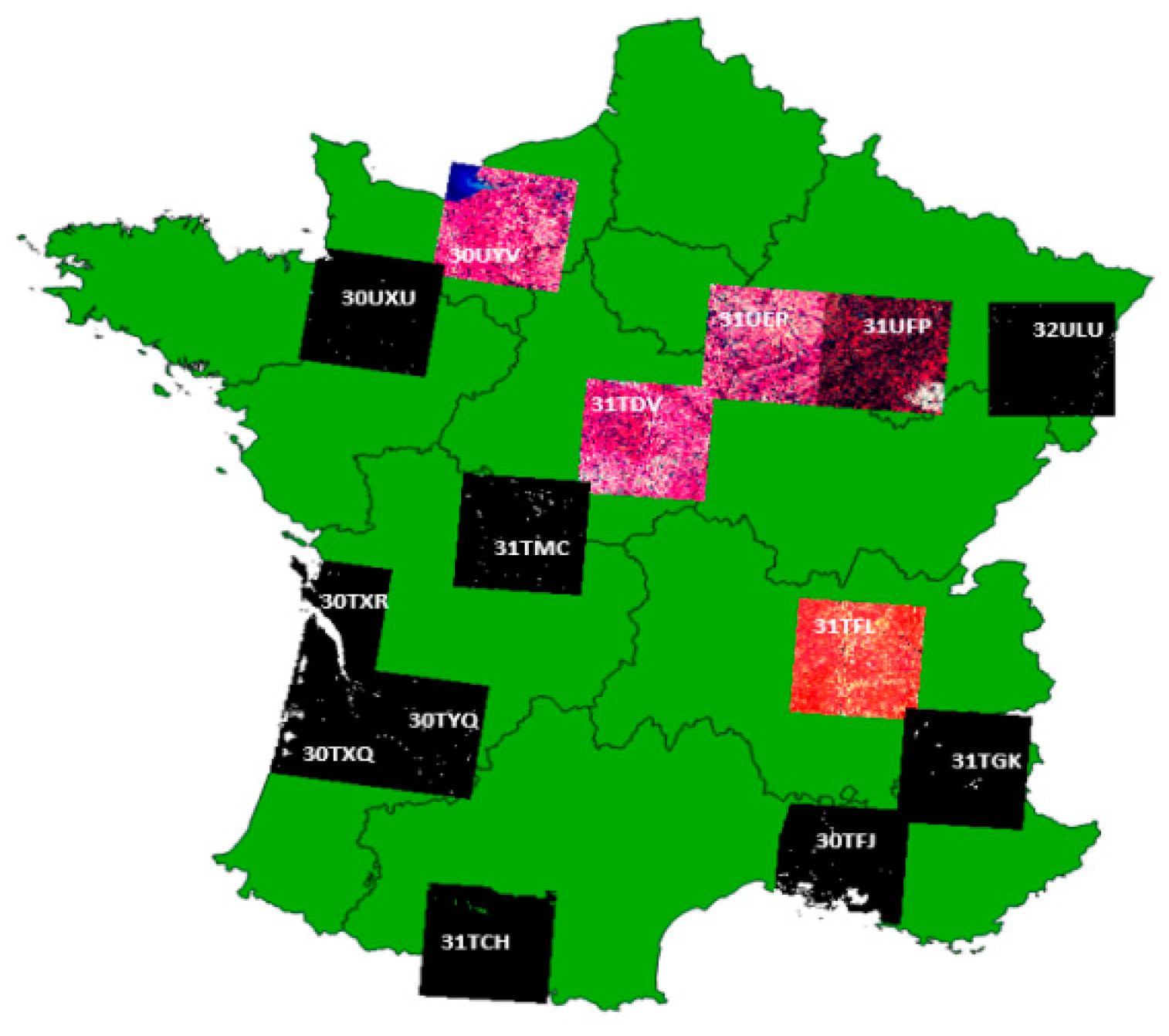
Figure 1. Water detection workflow on Sentinel1 and Sentinel2 observations, based on single and multiple date processes.
Remotesensing 13 03279 g001
Figure 2. 26 Large scene reference masks (110 × 110 km) have been generated over 14 sites in France.
Remotesensing 13 03279 g002
Figure 3. Reference reservoirs: (a) Surface dynamics over 3 years of in situ data (2017–2019), (b) Location of Reference Reservoirs in France (green).
Remotesensing 13 03279 g003
Figure 4. Representation of maximum extent (red), Convex hull (blue) and Eroded surface (green) for the following reservoirs: (a) Saint Géraud, (b) Tordre, (c) Pareloup, (d) Salagou.
Remotesensing 13 03279 g004
Figure 5. Satellite area estimations of Louet reservoir (Optical in orange, Radar in green) using 20 days time-window compared with the reference in-situ areas (blue line).
Remotesensing 13 03279 g005
Figure 6. Relative error of Reservoir area estimation using different combinations of optical and radar masks for 2 years of measurements at 29 instrumented reservoirs. Naming convention: MO = Optical, MR = Radar; MO1, MR1 = single date masks; MO2, MR2 = multiple dates masks; MO3, MR3 = maximum extent during the natural month; WN = N days of time-window length; avg = average logic; max = maximum logic. Optical methods have been represented in red tone boxes and radar methods in blue tone boxes. Multiple-date methods based on “maximum” logic are represented with more intense colors. Green horizontal lines inside the boxes show median values. The box is bounded at 25% and 75% quantiles and whiskers are set on 10% and 90% quantiles. Extreme values are represented as black circles.
Remotesensing 13 03279 g006
Figure 7. Relative error of Area estimation for High level reservoirs (>80% area quantile) measurements. See description at Figure 6 caption.
Remotesensing 13 03279 g007
Figure 8. Effect of dense vegetation and sandy surfaces on occurrence maps on the southern area of Miélan reservoir, where radar water detections are quite limited due to vegetation. (a) and background: ESRI aerial image; (b): water occurrence map from 2 year of optical observations; (c): water occurrence map from 2 year of radar observations. Zero occurrence has been displayed as transparent.
Remotesensing 13 03279 g008
Figure 9. Relative error of Area estimation for Low level reservoir measurements. See description at Figure 6 caption.
Remotesensing 13 03279 g009
Figure 10. Quantiles of absolute of relative error on area estimation on each method. (a) Quantile 50%; (b): Quantile 90%.
Remotesensing 13 03279 g010
Figure 11. Median Absolute of relative error of area estimations of reservoirs depending on their geomorphological indexes: maximum area, altitude, Eroded Area ratio, Convex-Hull Area ratio, Convex-Hull perimeter ratio and Eroded Perimeter ratio. (a) Results based in optical method “MO2_W20_avg” (b) Results based in radar method “MR_W20_avg”.
Remotesensing 13 03279 g011
Figure 12. Representation of the reference water mask on a specific date (red polygons) with ESRI Satellite background (a), compared with water occurrence map based on Optical measurements for 1 year of observations (b) and the water occurrence map based on Radar measurements for 1 year of observations (c).
Remotesensing 13 03279 g012
Figure 13. Impact of multi-temporal water detection on radar images. Top images show the improvement on water detection on rough waters on a large reservoir. Bottom images show the improvement on bare soils commission error. (a,e): GoogleMaps Satellite Image with reference water mask contour (red); (b,f): Reference water mask; (c,g): single-date radar water mask; (d,h): Multiple-date radar water masks (15 days) with average logic.
Remotesensing 13 03279 g013
Figure 14. Improvement of mean absolute of relative error between single date measurements (MO1, MR1) and multiple date (MO2_W20_avg, MR2_W20_avg) compared with the Number of observations on each reservoir for optical (a) and radar (b) measurements.
Remotesensing 13 03279 g014
Table 1. Description of the scenes used as reference with corresponding continental water surface in km2 and percentage.
RegionTileDatesWater Area
Km2 (%)
Scene Content
Alpes 131TGK24 February 201937.85 (0.31%)Snow, Mountain
Alpes 231TGL28 August 2018125.04 (1.03%)Mountain
Alsace32ULU12 September 201883.78 (0.69%)Lowlands, Slopes
21 Mars 2019100.14 (0.83%)Snow, Lowlands, Slopes
Ardèche31TFL17 February 2019122.75 (1.01%)Snow, Lowland, Slopes
24 Mars 2019119.75 (0.98%)Lowlands, Slopes
20 September 2019109.15 (0.90%)- 1
Ariège30TCH23 October 201839.94 (0.34%)Mountains
22 Mars 201931.42 (0.26%)Snow, Mountains
Bordeaux30TXQ11 September 2018187.36 (2.51%)Coast, turbid/clear water
23 February 2019184.40 (2.47%)-
Bretagne30UXU23 February 201954.93 (0.46%)Wetlands, small bodies
08 July 201839.94 (0.34%)-
Camargue31TFJ27 September 2018415.6 (4.14%)Coast, large water bodies
31 Mars 2019489.11 (4.71%)-
Chateauroux31TCM19 August 2018133.5 (1.1%)Lowlands
25 February 2019121.24 (1.0%)-
Gironde30TXR23 February 201992.63 (1.37%)Delta, turbid/clear water
Havre30UYV24 Mars 202085.91 (8.17%)Delta, lowlands
Marmande30TYQ22 February 201995.33 (0.79%)Wetlands, small bodies
Der Lake region31UFP10 July 2019173.5 (0.85%)Lowlands/gentle slopes
04 December 201945.38 (0.37%)-
29 December 2019121.86 (1.01%)Flood
Orient Lake region31UEP17 July 2019106.47 (0.88%) Lowlands/gentle slopes
04 December 201941.27 (0.37%)-
29 December 201981.65 (0.67%)Flood
Total 3239.90 (1.36%)—238,126 total surface
1 “-”: same as previous line.
Table 2. Geomorphological indexes derived from maximum extent surfaces for 4 different reservoirs. Maximum values are presented in bold style for each index (row).
Geomorphological IndexSaint GéraudTordrePareloupSalagou
Eroded Area Index 0.350.660.780.85
Eroded Perimeter Index 0.680.810.880.95
Convex Area Index 0.210.720.350.619
Convex Perimeter Index 0.620.790.400.69
Table 3. Median Scores for the Optical methods assessment and total number of failures (scenes with F1 < 0.5) for 74 scene evaluations. Best values are presented in bold style for each score (column).
Optical MethodSWIR FilterF1_ScorePrecisionRecallAccuracyFailures
Canny-Otsu MNDWI-0.8144960.9164220.8268360.996977
Canny-Otsu MNDWIYes0.8326460.928360.8260210.9972065
HSV-0.78840.916940.8757770.99611112
HSVYes0.8100960.9412630.8566480.9964877
Clustering 2 channelsYes0.8888890.9442920.8885260.9979966
Clustering 3 channels-0.8684140.8640120.9336130.9974167
Clustering 3 channelsYes0.8902390.8936920.9178150.9978144
Clustering 4 channelsYes0.8868540.9253460.8861620.9979396
Table 4. Median Scores for the Radar methods assessment and total number of failed comparisons (F1 < 0.5) for 123 scene evaluations. Best values are presented in bold style for each score (column).
Radar MethodLee Filter
-Size
Regularization
-Ball Radius
F1_ScorePrecisionRecallAccuracyFailures
Random ForestNo10.6810.6670.7160.99514
Random Forest3 × 310.6890.6740.7230.99520
Random ForestNo20.7270.7870.7100.9968
Table 5. Median Scores for Optical and Radar assessments on different multi-temporal window methods and lengths and number of failed scenes (F1 < 50%) over 74 optical scenes and 104 radar scenes. Best values are presented in bold style for each score (column).
Average Max
MethodF1_ScorePrecisionRecallAccuracyFailuresF1_ScorePrecisionRecallAccuracyFailures
Radar 1 day0.7270.7870.7100.996280.7270.7870.7100.9968
Radar 5 days0.7440.7890.7560.99610.7050.6690.7840.9953
Radar 10 days0.7950.8870.7540.997030.6720.5840.8100.9949
Radar 15 days0.7930.8900.7550.997030.5880.4920.8440.99323
Radar 20 days0.7970.8940.7520.997220.5650.4240.8620.99233
Radar 30 days0.8020.9070.7460.997320.5080.3860.8690.99046
Optical 1 day0.8900.8930.9170.997840.8900.8930.9170.99784
Optical 5 days0.8960.9060.8950.997990.8940.8700.9300.99787
Optical 10 days0.8990.8890.9030.9980100.8830.8340.9360.99759
Optical 15 days0.9010.9030.9040.9978100.8570.7860.9420.996610
Optical 20 days0.8860.8850.9150.997770.8460.7670.9600.996318
Optical 30 days0.8890.8990.8940.998170.8240.7400.9530.996414
Table 6. Effect of multiple-dates method compared to its corresponding single-date method on different evaluations.
Large Scene EvaluationReservoir Area Evaluation
OpticalRadarOpticalRadar
Multiple-dates Method Effect“Average” logicNeutralVery PositivePositivePositive
“Maximum” logicNegativeNegativePositiveVery Positive
Publisher’s Note: MDPI stays neutral with regard to jurisdictional claims in published maps and institutional affiliations.

