Article

A Practical Remote Sensing Monitoring Framework for Late Frost Damage in Wine Grapes Using Multi-Source Satellite Data

1
Key Laboratory of Environmental Remediation and Ecological Health, Ministry of Education, Zhejiang University, Hangzhou 310058, China
2
Institute of Applied Remote Sensing and Information Technology, Zhejiang University, Hangzhou 310058, China
3
Key Laboratory of Agricultural Remote Sensing and Information Systems, Hangzhou 310058, China
4
Spaider Information Technology Co., Ltd., Beijing 100086, China
5
Aerospace Newsky Technology Co., Ltd., Wuxi 214000, China
6
Xintianyuan Institute of Disaster Prevention and Reduction, Inner Mongolia, Hohhot 010051, China
7
School of Automation, Hangzhou Dianzi University, Xiasha Higher Education Zone, Hangzhou 310018, China
*
Author to whom correspondence should be addressed.
Remote Sens. 2021, 13(16), 3231; https://doi.org/10.3390/rs13163231
Submission received: 19 June 2021 / Revised: 6 August 2021 / Accepted: 10 August 2021 / Published: 14 August 2021
(This article belongs to the Special Issue Remote Sensing for Crop Stress Monitoring and Yield Prediction)

Abstract

:
Late frost damage is one of the main meteorological disasters that affect the growth of wine grapes in spring, causing a decline in wine grapes quality and a reduction in yield in Northwest China. At present, remote sensing technology has been widely used in the field of crop meteorological disasters monitoring and loss assessments, but little research has been carried out on late frost damage in wine grapes. To monitor the impact of late frost in wine grapes accurately and quickly, in this research, we selected the Ningxia planting area as the study area. A practical framework of late frost damage on wine grapes by integrating visible, near-infrared, and thermal infrared satellite data is proposed. This framework includes: (1) Wine grape planting area extraction using Gaofen-1 (GF-1), Landsat-8, and Sentinel-2 based on optimal feature selection and Random Forest (RF) algorithm; (2) retrieval of the land surface temperature (LST) using Landsat-8 thermal infrared data; (3) data fusion using Landsat-8 LST and MODIS LST for a high spatiotemporal resolution of LST with the Enhanced Spatial and Temporal Adaptive Reflectance Fusion Model (ESTARFM); (4) the estimation of daily minimum air temperature (Tmin) using downscaled LST and meteorological station data; (5) monitoring and evaluation of the degree of late frost damage in wine grapes in April 2020 by combining satellite-derived data and late frost indicators. The results show that the total area of wine grapes extracted in Ningxia was about 39,837 ha. The overall accuracy was 90.47%, the producer’s accuracy was 91.09%, and the user’s accuracy was 90.22%. The root mean square (RMSE) and the coefficient of determination (R2) of the Tmin estimation model were 1.67 ℃ and 0.91, respectively. About 41.12% of the vineyards suffered severe late frost damage, and the total affected area was about 16,381 ha during April 20–25, 2020. This suggests the satellite data can accurately monitor late frost damage in wine grapes by mapping the wine grape area and estimating Tmin. The results can help farmers to take remedial measures to reduce late frost damage in wine grapes, and provide an objective evaluation of late frost damage insurance claims for wine grapes. With the increasing weather extremes, this study has an important reference value for standardized global wine grape management and food security planning.

1. Introduction

Grape is one of the most productive fruits with a wide range of cultivation around the world, 80% of which are wine grapes. In evaluations of high-quality wine grape ecological regions, the Ningxia planting area has been classified as one of the best wine grape ecology districts in the world [1]. However, due to its location in the inland northwest, which has frequent cold air activity and temperature fluctuations in spring [2], this district is extremely vulnerable to low temperatures and late frost damages. Late frost damage seriously restricts the development of the local wine grape industry, yield, and quality stability [3]. Traditionally, monitoring and assessment of late frost damage in wine grapes have been based on meteorological stations and field investigations [4,5], but this progress is time-consuming, labor-intensive, and very expensive. Large-area and full-coverage remote sensing technology provide the promising potential for the monitoring and assessment of late frost damage as the remote sensing data can be used to extract the crop planting area [6,7,8,9,10], estimate the air and soil temperature [11,12], monitor the crop growth [13,14], assess the agro-meteorological disasters [15,16,17], and predict crop yields [18,19,20].
The wine grape planting area is the essential information for accurately monitoring and assessing late frost damage in wine grapes. Satellite data have been widely used to extract the planting area of crops, such as paddy rice [6,10,21,22], corn [7], wheat [23], and soybean [24] with high to medium spatial resolution [25,26]. However, little research has been carried out on extracting the wine grape planting area using high and medium spatial resolution satellite data, and the few studies mainly focused on small-scale research, such as vineyards [27] or at county scales [28]. From using single images [29,30] to multi-source satellite images [22,31,32], the combination of multiple types of data and features, such as sensitive bands, texture features, and vegetation index, can further provide comprehensive information and accurate extraction [23,33]. Several machine learning methods have been used in planting area extraction, such as maximum likelihood [24], support vector machine [34], and Random Forest (RF) [35,36]. The RF model [37,38] has also been widely used to optimize features and remove redundant information. Ningxia was selected as the study area in this paper as it is one of the most important cultivation areas of wine grapes.
Land surface temperature (LST) is an important parameter for late frost monitoring and evaluation [39]. The representative algorithms for LST derived from satellite data mainly include the Jiménez-Muñoz single-channel algorithm [40], the Qin mono-window algorithm [41], the Rozenstein split-window algorithm [42], and the Sobrino radiation transfer equation method [43], etc. These algorithms have widespread applicability [44], and are relatively mature. The spatial resolution of Landsat-8 thermal infrared data is 100 m, but its revisit period is 16 d. MODIS products can provide daytime and nighttime LST from the Terra and Aqua satellite, but their spatial resolution is 1 km. As the area of most wine grape plantations in the study area is less than 1 km2, the higher the spatial and temporal resolution, the better for late frost damage monitoring and assessment. Data fusion was used to produce data with high spatial and temporal resolution. Scholars have proposed a variety of downscaling methods for LST, including the Disaggregation Procedure for Radiometric Surface Temperature (DisTrad) [45], the Algorithm for Sharpening Thermal Imagery (TsHARP) [46], the High resolution Urban Thermal Sharpener (HUTS) [47], etc. The spatio-temporal fusion method has been a research hotspot in recent years, and scholars have carried out extensive research on this issue. The Spatial and Temporal Adaptive Reflectance Fusion Model (STARFM) [48], the Spatial Temporal Adaptive Algorithm for Mapping Reflectance Change (STAARCH) [49], the Enhanced Spatial and Temporal Adaptive Reflectance Fusion Model (ESTARFM) [50], and other fusion methods [51,52,53] were proposed accordingly. In comparison, the ESTARFM takes the heterogeneity of the pixels into account by introducing the conversion coefficients between pure and mixed pixels, which has high fusion accuracy in areas of high heterogeneity [54].
Air temperature is a physical parameter that is often used as the distinguishing factor for low-temperature freezing damage in crops. Since the daily minimum air temperature (Tmin) is one of the important indicators of agro-meteorological disasters, LST needs to be converted to Tmin. Obtaining continuous temporal and spatial daily Tmin images is the research focus of damage monitoring. Although the observational air temperature of traditional ground meteorological stations usually has high accuracy, due to the limited quantity and uneven distribution of meteorological stations, they cannot meet the demand for spatial continuity. Common remote sensing estimation methods for air temperature include statistical methods, the Temperature-Vegetation Index (TVX) [55], the atmospheric temperature profile method, and the energy balance method, etc. In recent years, based on the correlations [11,56] between air temperature and LST, the method of estimating air temperature by using full coverage LST has been recognized widely.
As current wine grape late frost damage monitoring is relatively sparse distributed, we proposed a practical remote sensing monitoring framework to monitor late frost damage in wine grapes and estimate the damaged area at a large scale. Specifically, this framework includes extraction of the wine grape planting area using Gaofen-1 (GF-1), Landsat-8, and Sentinel-2 satellite data; retrieval of LST using the Landsat-8 satellite data; fusion of Landsat LST and MODIS LST data; and estimation of daily Tmin. Ultimately, the spatial distribution and the degree of late frost damage in wine grapes were realized according to the disaster indicators, the results of extracting grape planting area, and the daily Tmin estimation.

2. Materials and Methods
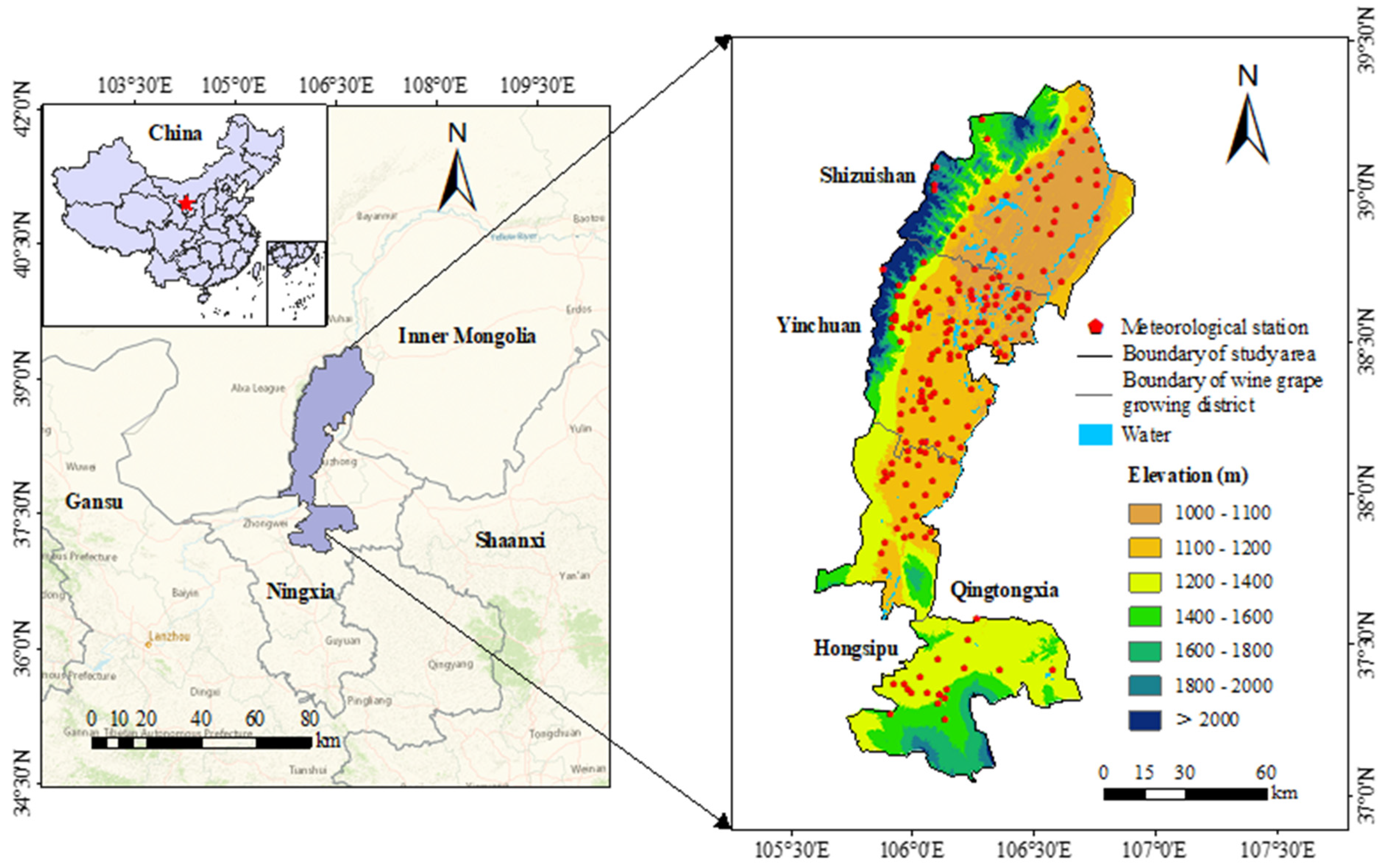
2.1. Study Area

Located in the Ningxia Hui Autonomous Region of Northwest China, the study area along the Helan Mountain extends from 37.47°N to 39.42°N and 105.62°E to 106.72°E (Figure 1). The Ningxia wine grape planting area includes four growing districts: Shizuishan, Yinchuan, Qingtongxia, and Hongsipu. It lies the temperate continental climate zone, with an average annual temperature range of 8–10 °C and an average annual precipitation range of approximately 130–250 mm. The annual sunshine hours are up to 3000 h, and the frost-free period is about 150 days.
With moderate heat and abundant sunshine, the study area has a typical continental climate, which is very conducive to the accumulation of sugar and the transformation of pigment, making it one of the major wine grape planting areas of China and world-recognized “golden area” and “Chinese Bordeaux” for wine grape cultivation. Through field surveys, it was found that the main phenology of wine grape (Figure 2) growth is from April to August, with the harvest period from September to October and the overwintering period from November to March of the next year.

2.2. Satellite Data and Preprocessing

The satellite data used in this paper can be divided into two parts: (1) GF-1, Landsat-8, and Sentinel-2 data for extracting wine grape planting area; and (2) Landsat-8 thermal infrared data and the MODIS product set (LST and EVI) for LST retrieval and data fusion.
Sentinel-2 images are provided freely by the European Space Agency (ESA) scientific data hub portal (https://scihub.copernicus.eu/, accessed on 31 May 2020). Landsat-8 images are freely available for users to download from the United States Geological Survey (USGS) website (https://earthexplorer.usgs.gov/, accessed on 1 June 2020). GF-1 satellite images are provided freely by the China Centre for Resources Satellite Data and Application (CRESDA) (http://www.cresda.com, accessed on 12 April 2020). GF-1 is the first satellite of a series of high-resolution earth observation systems from China, launched in April 2013. GF-1 Wide Field of View (WFV) images have an overlapping swath of 830 km and contain four bands (blue, green, red, and near-infrared) with a spatial resolution of 16 m. MODIS products are freely available to users via the National Aeronautics and Space Administration (NASA) satellite data website and can be downloaded from https://ladsweb.modaps.eosdis.nasa.gov/search/ (accessed on 3 July 2020).
To obtain enough images to cover the main phenological stages of wine grape in the study area, 10 cloud-free multi-source satellite images from April 2019 to April 2020 were used to extract the planting area, and they included two GF-1 WFV images with a spatial resolution of 16 m, four Landsat-8 Operational Land Imager (OLI) images with a spatial resolution of 30 m and four Sentinel-2 Multispectral Instrument (MSI) images with a spatial resolution of 10 m (Table 1).
Three cloud-free Landsat-8 Thermal Infrared Sensor (TIRS) images were acquired on 22 March, 23 April, and 9 May 2020 at a spatial resolution of 100 m. Thirty Aqua MODIS images of nighttime LST (MYD11A1) from 1 April to 30 April 2020; three images of daytime LST (MOD11A1) on 22 March, 23 April, and 9 May 2020; and seven MODIS images of EVI products (MOD13A2.A2020081/A2020097/A2020113/A2020129, MYD13A2.A2020089/A2020105/A2020121) were acquired with a spatial resolution of 1 km.
The FLAASH module [57] of ENVI was used for atmospheric correction of the GF-1 and Landsat-8 images, and the sentinel-2 images were preprocessed by Sen2Cor (http://step.esa.int/main/third-party-plugins-2/sen2cor/, accessed on 5 June 2020). and used as reference images to geometrically correct the GF-1 images from the same day. The GF-1 and Sentinel-2 images were all resampled to 30 m spatial resolution. The digital elevation model (DEM) used in preprocessing was Shuttle Radar Topography Mission (SRTM) DEM. All MODIS products downloaded used the MODIS Reprojection Tool (MRT) provided by NASA for reprojection, data layer extraction, and format conversion (HDF to TIF).

2.3. Meteorological Data

In this study, daily Tmin data from 1 April to 30 April 2020 were collected from 180 meteorological stations (Figure 1) in the study area. The LST values used as validation data on April 2020 were acquired from the Real-Time Product Dataset of the China Meteorological Administration Land Data Assimilation System (CLDAS-V2.0), which were downloaded from China meteorological data service center (CMDC) (http://data.cma.cn/, accessed on 15 October 2020).

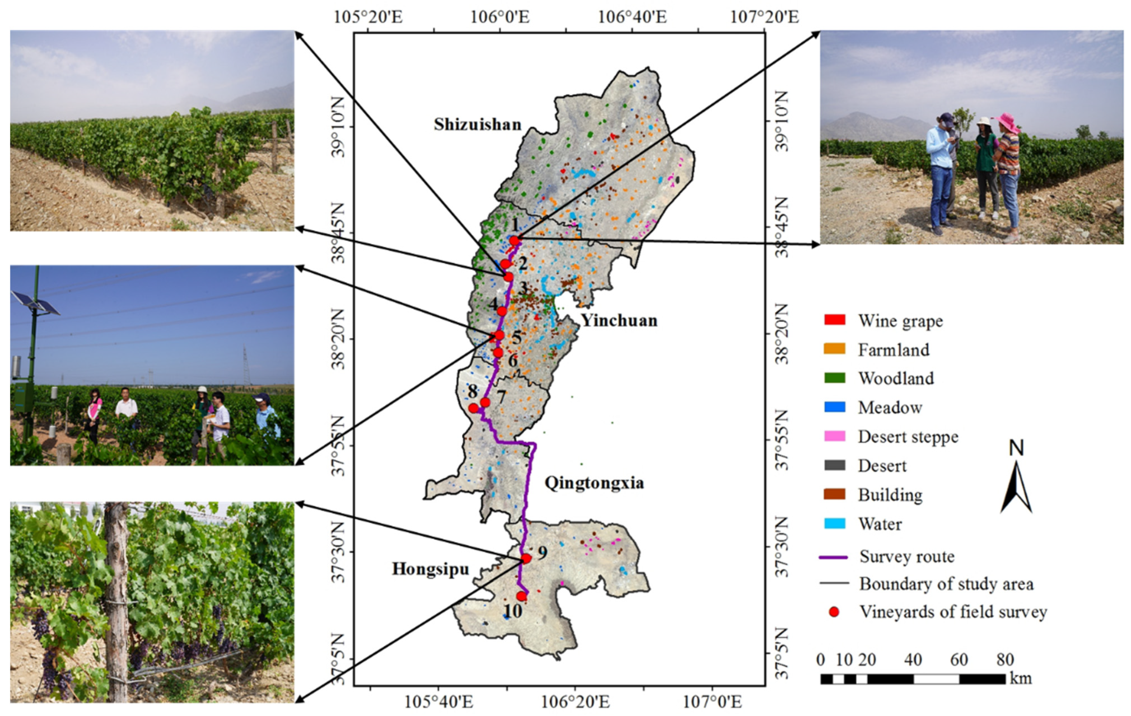
2.4. Field Survey and Sample Set

The field survey was carried out from July 30 to August 3 in 2019. We visited 10 vineyards in Yinchuan, Qingtongxia, and Hongsipu to collect information about the wine grape distribution, grape species, and cultivation measures in the study area. Based on the field survey and visual interpretations of Google Earth, more than 2000 samples (consisting of over 150,000 pixels) of wine grapes, farmland, woodland, meadow, desert steppe, desert, building, and water were selected as training and validating samples (Figure 3). In this study, 60% were used as training samples; the remaining 40% were used to validate and evaluate the extraction results.

2.5. Methods

The framework proposed in this study is presented in Figure 4. Firstly, the wine grape planting area was extracted by optimal feature selection and the RF method. Secondly, Landsat-8 LST (using two retrieval algorithms) and MODIS LST (after cloudy gap-filling) were fused to obtain a seamless daily high spatial resolution of LST (100 m). Thirdly, fully covered Tmin was estimated based on the correlations between downscaled LST and meteorological station Tmin data. Finally, by using daily Tmin images of the study area, wine grape planting area image, and the evaluation indicator of wine grape late frost damage, we obtained a map of the late frost damaged area of wine grapes in the study area in April 2020.

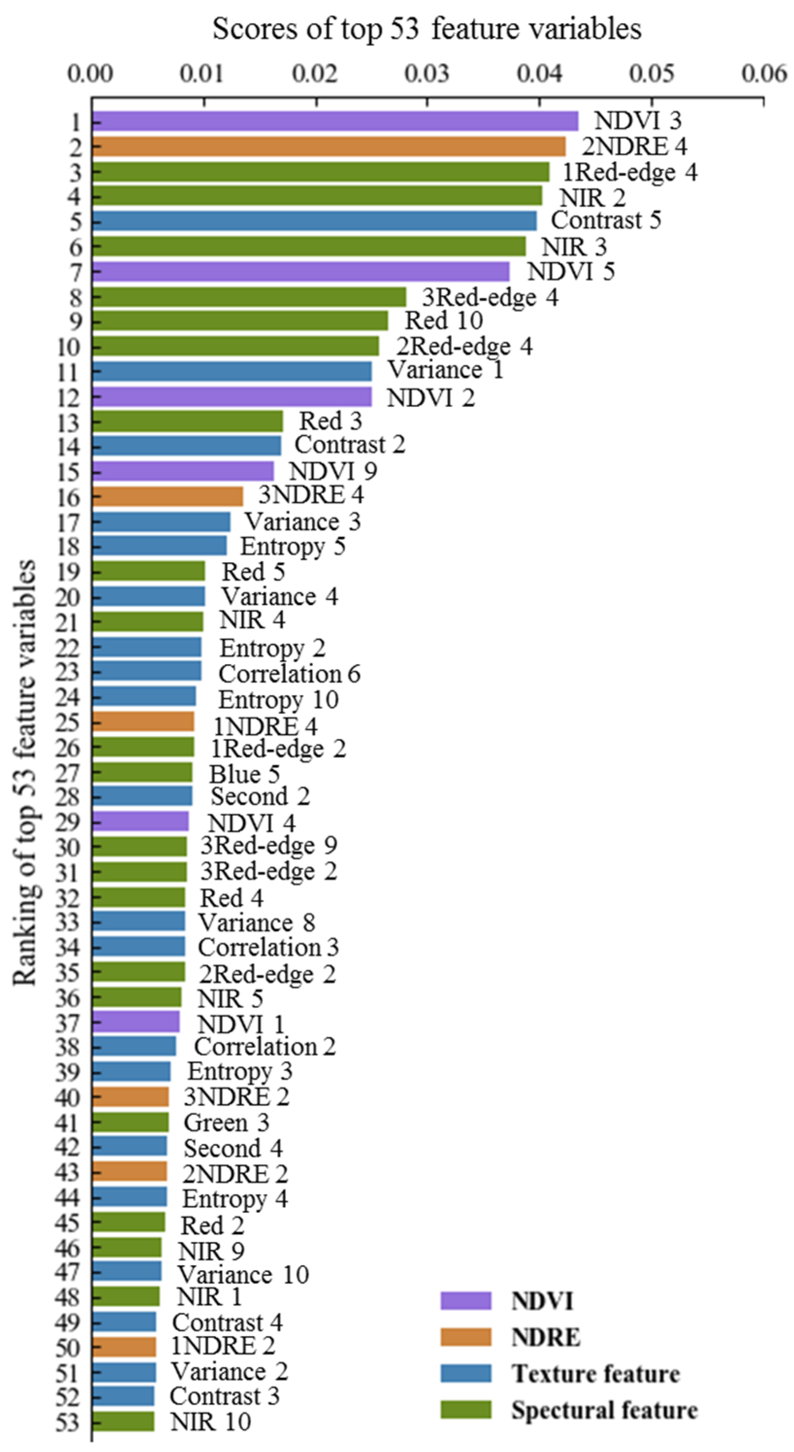
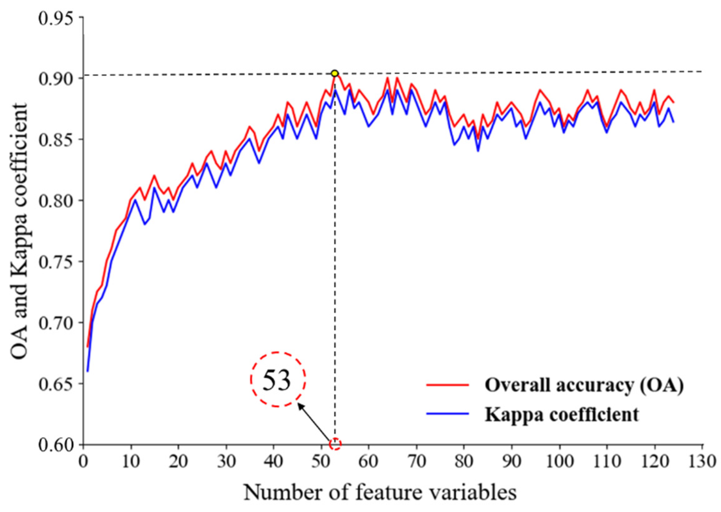
2.5.1. Extraction of the Wine Grape Planting Area Using RF

RF is a machine learning algorithm that uses multiple decision trees to train and predict samples. It was first proposed by Breiman [58]. This method can effectively solve the over-fitting phenomenon by double random sampling of the training samples and selected feature variables and constructing multiple decision trees through the idea of integrated learning. Each decision tree grows to the maximum without any pruning. Through internal evaluation, the unbiased error is estimated in the process of RF generation, and the final prediction and classification results depend on the mean prediction value and the voting results of multiple decision trees.
In this study, the RF algorithm and Gini index were used to evaluate the importance of features and determine the optimal feature subset according to the voting mechanism [59]. Gini index evaluates the classification contributions of the feature variables in each tree of RF, normalizes all the feature importance scores, and compares the feature importance weights. The Python language and the Scikit-learn library were used to implement the feature optimization progress [60].
Different crops show different spectral characteristics, due to their different pigment and moisture content and different canopy structures [61]. Therefore, spectral features can be used for crop recognition. In total, 52 spectral features were obtained from 10 multi-source satellite images, including eight bands (Blue, Green, Red, Near-infrared) of two GF-1 images, 16 bands (blue, green, red, and near-infrared) of four Landsat-8 images, and 28 bands (blue, green, red, near-infrared, and three red-edge bands) of four Sentinel-2 images.
The vegetation indices were calculated from different spectral reflectance for vegetation discrimination and quantitative retrieval of parameters. NDVI is one of the most important indices for deriving crop phenological parameters and distinguishes different types of ground objects, which can reflect the difference between the vegetation and soil and is suitable for dynamic monitoring during early growth stages. As a common indicator parameter of green plants, the Normalized Difference Red Edge Index (NDRE) has a high sensitivity for vegetation recognition and classification, as it can take advantage of the red-edge bands in the field of agricultural remote sensing monitoring [62]; it is widely used in agriculture and forest monitoring. In this study, NDVI values were calculated from the 10 multi-source satellite images. Sentinel-2 contains three red-edge bands, so 12 NDRE features were calculated from the four Sentinel-2 images. NDRE features were not calculated from the GF-1 and Landsat-8 images, due to their lack of red-edge bands.
Texture features measures the surface roughness and uniformity of image pixel by the similarity of spatial structure, reflecting the close relationship between texture information and gray-scale [63], which has become one of the major factors in image classification [64]. The Principal Component Analysis (PCA) transformation was implemented on the spectral bands of 10 images, and only the first PCA, which had the highest amount of information, was selected to calculate five texture features based on the Gray Level Co-occurrence Matrix (GLCM). The five texture features were variance, contrast, correlation, angular second moment, and entropy.
In total, 124 features were obtained from the NDVI, NDRE, spectra, and texture data, from which the feature set was selected, as listed in Table 2.

2.5.2. Data Fusion of LST

The mono-window algorithm (LST_MW) [65], and the nonlinear split-window algorithm [66] were utilized to calculate LST using Landsat-8 TIRS on 22 March, 23 April, and 9 May 2020, respectively. The LST_MW constructs the calculation model of LST, atmospheric transmittance, brightness temperature, and average atmospheric temperature based on the thermal radiation transfer equation and Landsat-8 TIRS 10. The split-window algorithm (LST_SW) used the atmospheric absorption difference between the two thermal infrared channels to correct the atmospheric impact, establishing the relationship between the LST and the brightness temperature.
The MODIS LST products with a temporal resolution of 1 day provided an excellent source for the temporal continuity analysis of LST. Since wine grape late frost damage usually occurs during 03:00–04:00, which is close to the observation time of the Aqua MODIS nighttime LST (MYD11A1), MYD11A1 products were selected as the data source for LST with a high temporal resolution of 1 day and a low spatial resolution of 1 km. However, the quality of pixels largely depends on the cloud coverage, so cloudy weather may lead to poor pixel quality. Since the Helan Mountain lies to the west of the study area, which is affected by snow accumulation in early spring, the mountainous area often has many low-quality pixels. In this study, the spatiotemporal linear interpolation method was used to find similar properties between the effective pixels and invalid pixels (the pixels with poor quality were removed) in the adjacent time and space; then, the missing pixels were interpolated by calculating the conversion relationship [67].
Assuming that the LST of similar pixels can be known at time t 0 and t 1 , then the linear relationship between two LST images can be defined by statistical linear regression.
LST t 0 = f ( LST t 1 )
where LST t 0 is the LST at t 0 , and LST t 1 is the LST at t 1 . If the LST of the pixel at t 0 is unknown, but that at t 1 is known, then the LST of the pixel at t 0 can be obtained through the linear relationship above.
Given the cloud cover in the study area, LST images with cloud-free pixel coverage of more than 70% were selected as the reference image, and the image with cloud-free pixel coverage less than 70% as interpolated images. We then established the linear model linking the cloud-free pixels of the interpolated images, cloud-free pixels of the reference images, DEM and EVI. Due to the different measurements of LST, DEM, and EVI, the three values were normalized before establishing the linear relationship.
LST i n t = a LST r e f + b DEM + c EVI + d
where LST i n t is the array of interpolated images, LST r e f is the cloud-free pixel array of reference image, and a, b, c, and d are regression coefficients. With this equation, the LST pixels of cloud cover can be calculated using the reference images, DEM and EVI. For the missing pixels after filling, the CLDAS-V2.0 0 cm LST data set was used for further filling. The downloaded CLDAS-V2.0 0 cm LST can be used as supplementary data after format conversion, coordinate system conversion, resampling, clipping, and other processing.
To obtain LST with a high spatiotemporal resolution, ESTARFM was used to fuse the Landsat-8 LST and MODIS LST. ESTARFM is a data fusion algorithm based on a moving window [54,68]. It is based on the premise that the image registration of fine-resolution and coarse-resolution images is accurate, and it is assumed that the reflectivity difference between the images is only caused by system deviation, and there is no significant difference between the images from two periods [50,69]. The satellite images used for downscaling model are listed in Table 3.
Assuming that the land cover types and the sensor calibration of the two images are consistent, the relationship between fine-resolution (Landsat-8 LST) and coarse-resolution (MODIS LST) images can be described by a linear model.
L ( x , y , t l , B ) = a M ( x , y , t l , B ) + b
L ( x , y , t p , B ) = a M ( x , y , t p , B ) + b
where L ( x , y , t l , B ) and M ( x , y , t l , B ) are the pixel values of Landsat-8 LST and MODIS LST at t l , L ( x , y , t p , B ) and M ( x , y , t p , B ) are the pixel values of Landsat-8 LST and MODIS LST at t p , and a and b are conversion coefficients of the linear regression model and depend on the system deviation of the sensor.
Equation (5) can be derived from Equations (3) and (4):
L ( x , y , t p , B ) = L ( x , y , t l , B ) + a [ M ( x , y , t p , B ) M ( x , y , t l , B ) ]
Because of the complexity of the land surface, most of the pixels in the images are mixed pixels, that is, one pixel contains different land cover types. It is difficult to ensure the accuracy of the prediction results by using only a single pixel. Therefore, assuming that the reflectivity of the mixed pixels is a linear combination of that in different land cover types, and that the proportion of land cover types in the two images remains basically unchanged, the reflectivity of the mixed pixel can be expressed as:
L ( x , y , t p , B ) = L ( x , y , t l , B ) + v ( x , y ) [ M ( x , y , t p , B ) M ( x , y , t l , B ) ]
where v ( x , y ) is the conversion coefficient of mixed pixels.
According to the principle that the similar neighboring pixels have similar reflectivity, a moving window is used to obtain the information of the neighboring pixels, and the information of the similar pixels is then integrated into the calculation of fine-resolution reflectivity. From the similarity between neighboring pixels, the central pixel values of the predicted images are calculated as follows:
L ( x w / 2 , y w / 2 , t p , B ) = L ( x w / 2 , y w / 2 , t l , B ) + i = 1 N W i V i [ M ( x i , y i , t p , B ) M ( x i , y i , t l , B ) ]
where ( x w / 2 , y w / 2 ) is the location of the central pixel, w is the size of the moving window, N is the number of similar pixels, including the central predicted pixel, W i is the weight of the ith similar pixel, V i is the conversion coefficient of the ith similar pixel, and ( x i , y i ) is the location of ith similar pixel.
Two images from different dates were used to calculate the value of the center pixel. Landsat-8 LST and MODIS LST images at t m and t n were used to predict the fine-resolution reflectance of date t p , and the weighted combination of the two prediction results was calculated to obtain a more accurate value. The temporal weight was calculated by the magnitude of change in the MODIS values between t l (l = m, n) and t p , and Equation (8) is as follows:
T k = 1 / j = 1 W i = 1 W M ( x i , y i , t l , B ) j = 1 W i = 1 W M ( x i , y i , t p , B ) k = m , n ( 1 / | j = 1 W i = 1 W M ( x i , y i , t l , B ) j = 1 W i = 1 W M ( x i , y i , t p , B ) | ) ,   l = m , n
Then the final predicted fine-resolution reflectance of the center pixel at t p is as follows:
L ( x w / 2 , y w / 2 , t p , B ) = T m L m ( x w / 2 , y w / 2 , t m , B ) + T n L n ( x w / 2 , y w / 2 , t n , B )
where L m ( x w / 2 , y w / 2 , t m , B ) and L n ( x w / 2 , y w / 2 , t n , B ) are fine-resolution pixel value, respectively, at t m and t n , and T m and T n are the temporal weight of t m and t n .

2.5.3. Estimation Model of Daily Minimum Air Temperature

The daily Tmin was estimated by the 30 images of downscaled LST (LSTE) in April 2020 with the spatial resolution of 100 m. The observation time for MODIS LST was 1:30 a.m. every day, and the late frost of wine grapes often occurs during 03:00–04:00, and the daily Tmin in the study area occurs during approximately 05:00–07:00 [4]. The research showed that temperature at these key times had a strong linear correlation, so we can monitor the late frost damage by building a linear estimation model. Because LSTE was calculated from MODIS LST, LSTE is considered to have a similar property with MODIS LST and also has a good linear relationship with the daily Tmin. Therefore, the study constructed a linear model of the daily Tmin and LSTE to estimate the daily Tmin using Equation (10). The daily Tmin in April 2020, as input variable in the model, was derived from meteorological stations.
T min = a LST E + b
where a and b are the regression coefficients of ordinary least squares regression.

2.5.4. Mapping the Late Frost Damaged Area

The evaluation indicators of wine grape late frost damage from the Yinchuan Meteorological Bureau (Figure 4), were proved to be reliable through experiments and verification. The occurrence of wine grape late frost damage is related to air temperature, precipitation, and soil conditions, but the low air temperature is the most important factor. In this study, we classified the degree of late frost damage according to the evaluation indicator and the daily Tmin of each wine grape pixel.
As described in Section 2.5.1 and Section 2.5.3, daily minimum air temperature images (DMTI), wine grape planting area image (WGPAI), and the evaluation index of wine grape late frost damage (LFDEI) were obtained and integrated to derive the late frost damage images (LFDI) [17]. Equation (11) is as follows:
LFDI = ( DMTI ) ( WGPAI ) ( LFDEI )
The spatial distribution information of late frost damage was then further combined with the estimated area of wine grapes to estimate the late frost damaged area in the Ningxia planting area in April 2020.

3. Results

3.1. Extraction of the Wine Grape Planting Area

In total, 124 features, including spectral reflectance, vegetation indices, and texture features, were calculated. Rankings of the feature importance and performance are shown in Figure 5, and the changes in the overall accuracy (OA) and kappa coefficient with the number of feature variables are shown in Figure 6.
The OA and the kappa coefficient first increased rapidly with the number of feature variables (Figure 5), then, increased slowly and fluctuated up to 13 features. When the number of features reached 53, the total accuracy and kappa coefficient value reached the maximum. Therefore, the top 53 features were used as the optimal feature subset to extract wine grape planting area. Among the top 53 features (Figure 6), which included 21 spectral features, 20 texture features, and 12 vegetation index features (6 NDVI features and 6 NDRE features), NDVI 3 had the highest feature importance score, and NIR 10 had the lowest.
Based on the testing samples, the extraction results were assessed using the confusion matrix with OA, producer accuracy (PA), user accuracy (UA), and the kappa coefficient of the optimal feature subset in Table 4.
The OA and kappa coefficient were 90.47% and 0.89, respectively. The wine grape PA and UA were 91.09% and 90.22%, respectively. The omission and commission error may have been caused by mixed pixels around the vineyard border, due to the limitation of the spatial resolution of the satellite images. On the other hand, wine grapes in new plantations can be classified as desert, due to their low vegetation coverage and similarity to bare soil. The extracted area of wine grape planting regions (Figure 7) was calculated to be about 39,837 ha.

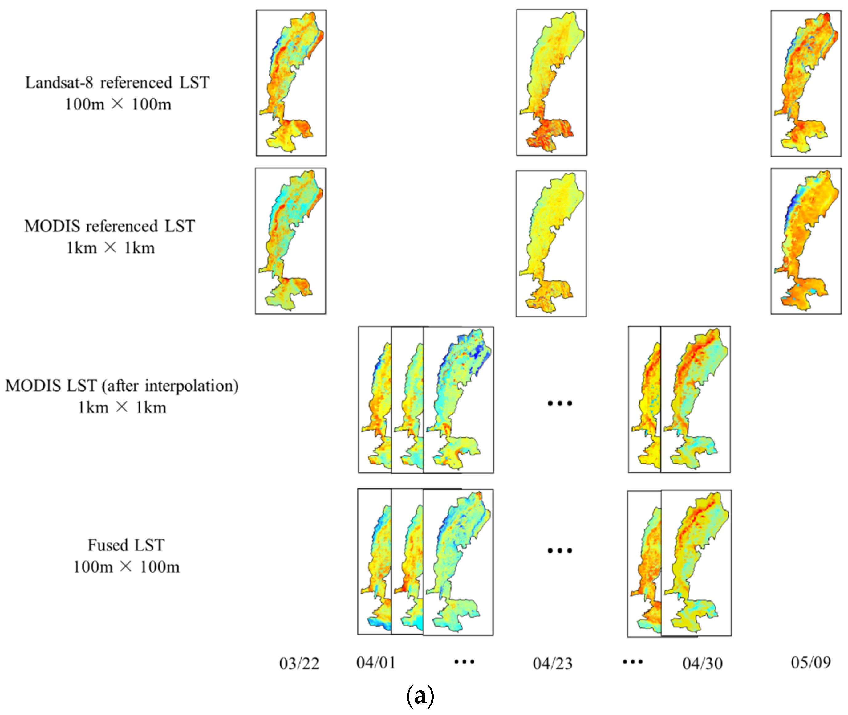
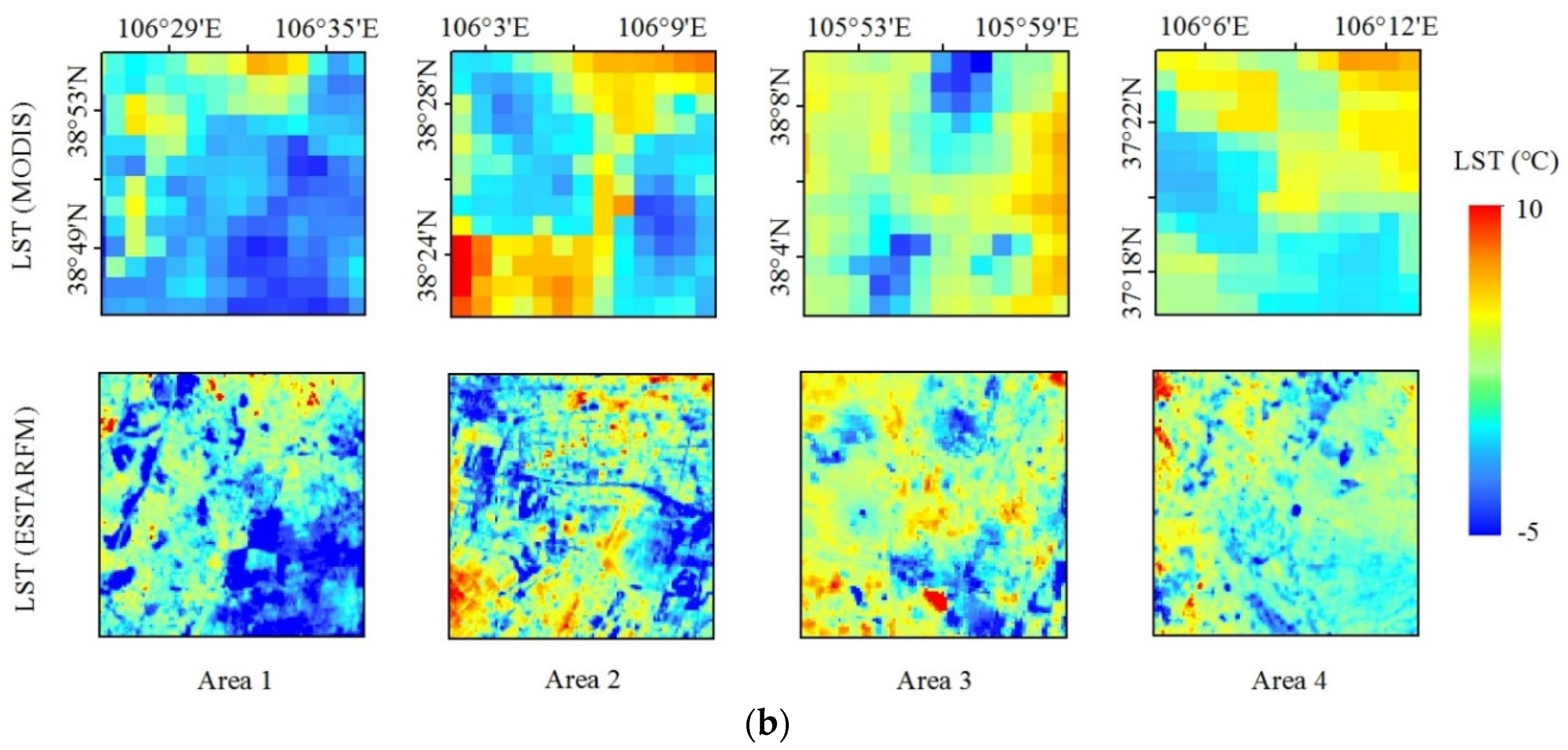
3.2. Data Fusion of Landsat-8 LST and MODIS LST Using the ESTARFM Method

3.2.1. LST Retrieval Using Landsat-8 Thermal Infrared Data

The LST_MW and the LST_SW were used to retrieve the LST from Landsat-8 TIRS (TIRS 10: 10.60~11.19 μm; TIRS 11: 11.50~12.51 μm) at a resolution of 100 m. One hundred pixels were randomly selected from every LST_MW and LST_SW image. The verification pixels of three dates obtained by the same algorithm were combined into a group, with a total of 300 pixels in each group. Through a comparison with the corresponding pixel values of CLDAS-V2.0 at 11:00 (the observation time of Landsat-8 is about 11:30 a.m. Beijing time), the accuracy of the two LST retrieval algorithms was analyzed. Figure 8 shows the scatter plot of the LST calculated by the two algorithms versus CLDAS-V2.0 LST.
We revealed that in the scatter plot of the two groups of 300 verification pixels; the root mean square (RMSE) of LST_MW and LST_SW were 2.15 °C and 2.51 °C, respectively. In addition, the coefficient of determination (R2) of LST_ MW was 0.78, and the R2 of LST_ SW was 0.76. Based on the above analysis, although there were some differences between the two algorithms in the process of LST retrieval, the two algorithms both produced ideal retrieval results, and the accuracy of the LST_MW algorithm was relatively higher than that of the LST_SW algorithm in this study. Therefore, the LST calculated by the LST_MW algorithm was used for subsequent research.

3.2.2. Cloud Gap-Filling of MODIS LST Data

During April, the valid pixel rates of the original daily MODIS LST images in the study area were 8.77% to 82.95%. The cloud-free pixel coverage on 4, 11, 16, 26, 27, 28, and 30 April were 71.57, 79.46, 79.80, 82.95, 79.04, 71.65, and 80.85, respectively. Therefore, these LST images were selected as the reference image, and the others were interpolated images. The multivariate regression model was built by using the cloud-free pixels of the interpolated images as the dependent variables and the cloud-free pixels of the reference image, DEM and EVI, as the independent variables. The model increased the valid pixel rates of all interpolated images. The effect of pixel interpolation in daily MODIS LST images is shown in Figure 9. After interpolation, the valid pixel rates of all interpolated images were 71.57% to 86.40%.
The MODIS LST images in April were compared with the pixels of CLDAS-V2.0 LST as follows: All 30 images were taken as a group, randomly choose 50 interpolated pixels in each image; that is, 1500 random pixels were selected for the validation. We validated the cloud gap-filling methods (Figure 10); overall, the R2 between the interpolated MODIS LST and CLDAS-V2.0 LST was 0.87 with RMSE of 1.79 °C, which indicates a strong correlation between MODIS LST and CLDAS-V2.0 LST. Furthermore, for the pixels still vacant after interpolation, CLDAS-V2.0 0 cm LST real-time products were used to fill them indirectly, then the valid pixel rates of all images were 100%. The final nighttime LST images with full spatial coverage at 1 km resolution in the study area were obtained and used as the data source for the data fusion stage of the research.

3.2.3. Data Fusion of Landsat-8 LST and MODIS LST Using the ESTARFM Method

Temporal resolution changes before and after data fusion are shown in Figure 11a. Taking four 13 km × 13 km local areas in Figure 11b as an example, the spatial resolution results of data fusion can be visualized by comparing the differences in the LST image pixels before and after data fusion for 24 April.
Figure 11 shows the data fusion result of LST both in temporal and spatial resolution. In Figure 11a, only three images of Landsat-8 LST were used before data fusion. After fusion by ESTARFM, a complete data set containing 30 images of LST in April was obtained. In Figure 11b, compared with the LST images with a spatial resolution of 1 km, the downscaled images have more detailed information and a clear description of the LST pixels. With regard to the phenomenon of local blurring and mutation at the boundary of different types of ground objects, this study analyzed the reasons, which may be the degradation of the downscaling quality caused by the high degree of fragmentation of mixed pixels. Overall, downscaled LST had a high correlation with MODIS LST and could be used to construct the model of the following Tmin estimation.

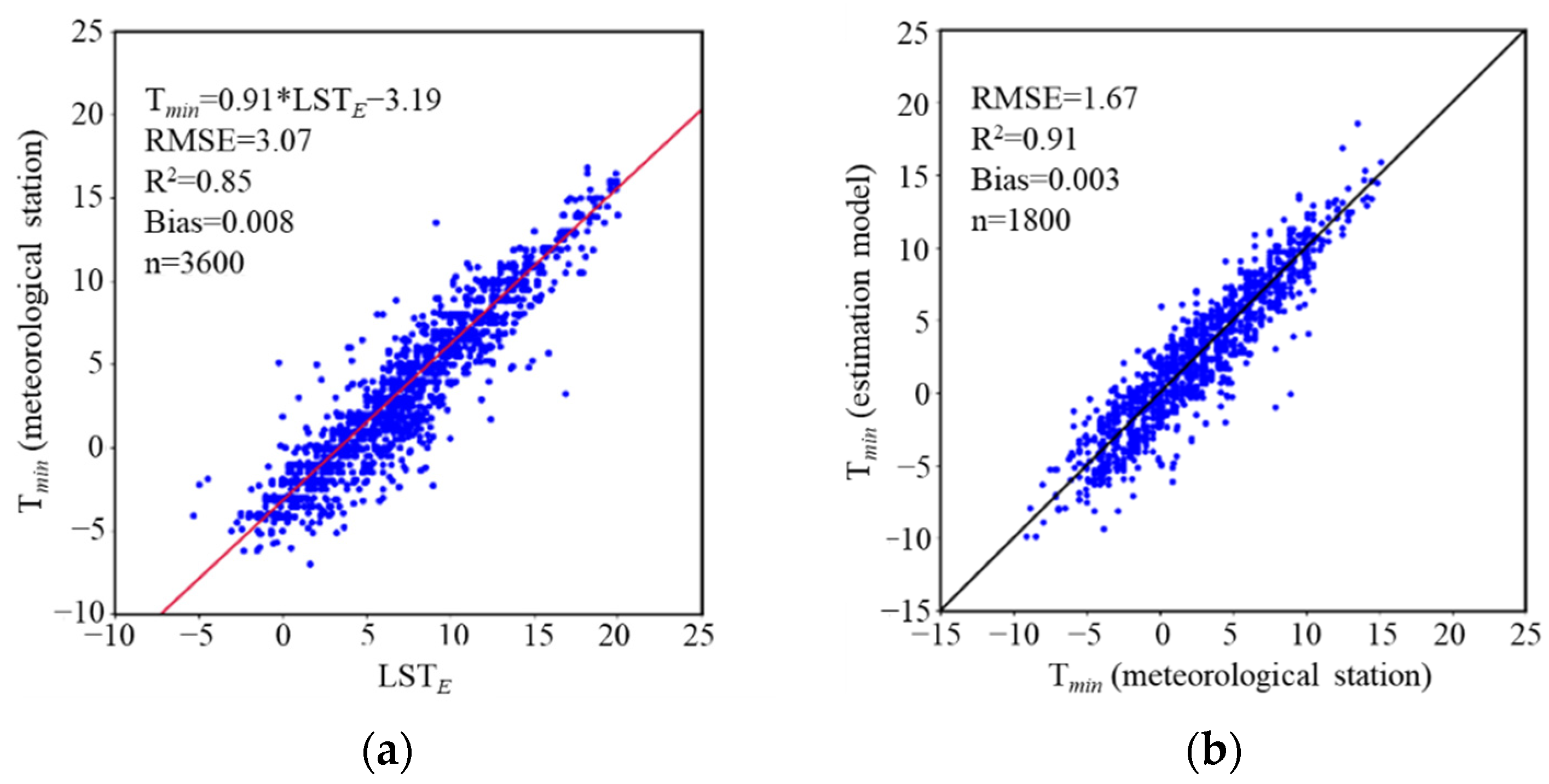
3.3. Calibration and Validation of Daily Minimum Air Temperature Estimation Using the Downscaled LST Data

A linear regression model was constructed between Tmin measured from 180 meteorological stations and the fused LSTE derived from the Aqua nighttime MODIS LST and Landsat LST. Two-thirds of the meteorological data were used for modeling and one-third for validation.
The regression model between Tmin and LSTE is formatted in Equation (12).
T min = 0.91 LST E 3 . 19
RMSE was 3.07 °C; the R2 and Bias for the estimation model of daily minimum air temperature were 0.85 and 0.008, respectively.
Fully covered Tmin of the study area can be calculated by Equation (12). In Figure 12b, the scattered points are distributed near the 1:1 line. The RMSE and R2 of the estimated Tmin and measured Tmin were 1.67 °C and 0.91, respectively. The low error value and good correlation indicated that the estimation model had high applicability for the estimation of Tmin in the study area, and the estimated results can be used for remote sensing monitoring and grade evaluation of wine grape late frost damage.

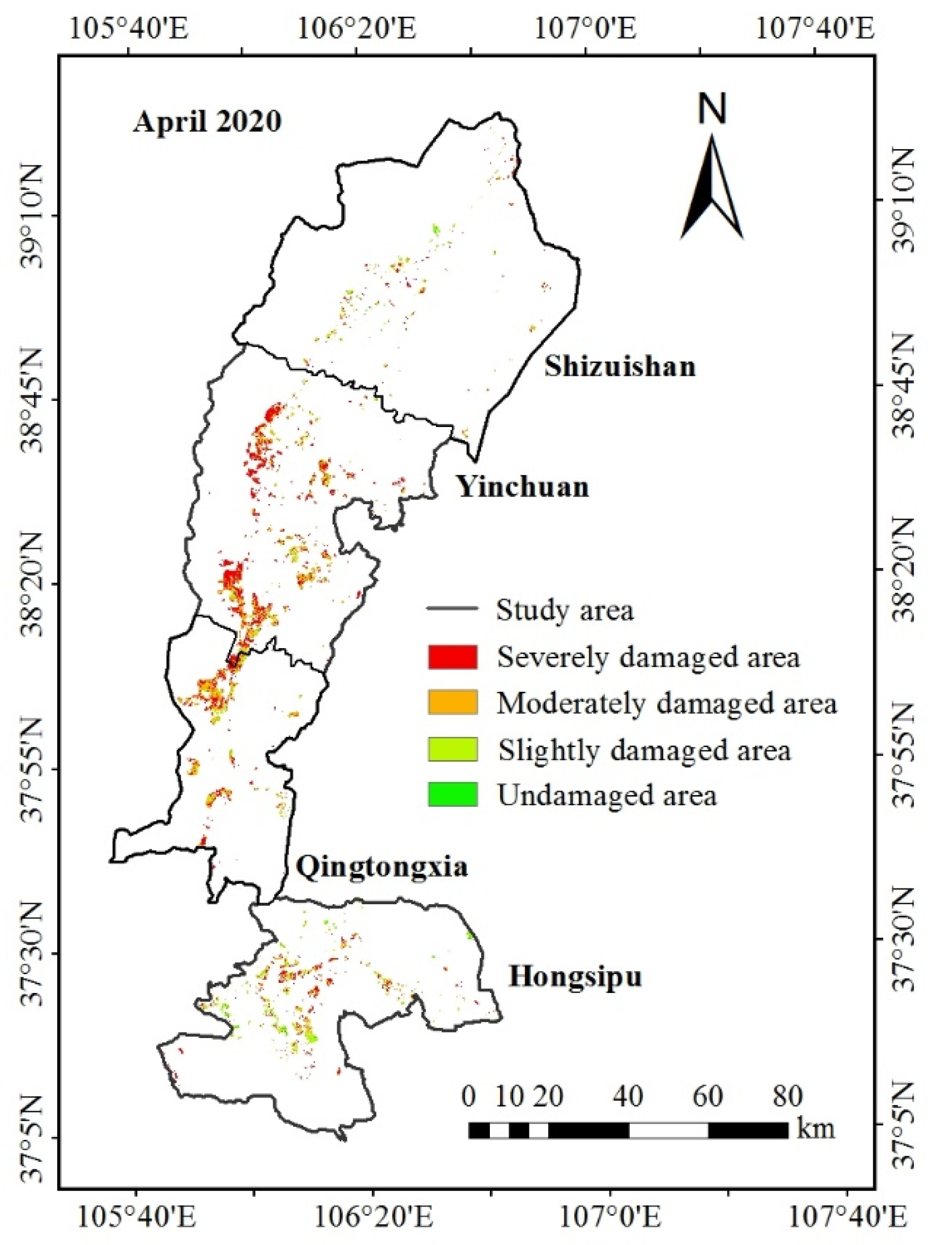
3.4. Mapping of the Late Frost Damaged Area

The distribution map of the wine grape planting area with a spatial resolution of 30m was resampled to 100 m, which was consistent with the spatial resolution of Tmin. The spatial distribution of wine grapes and full spatial coverage of Tmin at 100 m resolution in each planting region in April 2020 were combined to obtain the daily late frost damaged area. The results showed that in April 2020, affected by the very cold air, days with low air temperature appeared frequently and intensively. There were about 14 days when the daily Tmin was lower than 0 °C in the planting area; that is, there were 14 late frost days, which were 2–4 April, 11–13 April, 16–17 April, and 20–25 April. Among these days, extremely low air temperature appeared on the morning of 24 April, when the Tmin suddenly dropped to about −6 °C; the Tmin on the other days of the fourth late frost period were all below 0 °C. Although the Tmin was lower than 0 °C, most of the wine grapes were not frozen before 20 April because they had just been unearthed from the soil, but had not yet sprouted. This period had strong resistance to low air temperature, which had little effect on the growth of wine grape buds and leaves. Therefore, we monitored the late frost situation during 20–25 April.
Figure 13 shows the remote sensing monitoring of late frost in the wine grape planting area in April 2020. The severe damage area is mainly concentrated in the central part of the study area, with less frost damaged in the northern part. Combined with the local field survey, we found that the degree of late frost damage was relatively severe in areas with low or flat terrain. Table 5 shows the affected area during the late frost damage in April 2020. We found that a total of 77.48% of the vineyards suffered from late frost damage, and the area of wine grapes affected by severe late frost damage reached 16,381 ha, accounting for 41.12% of the total planting area. Among the areas, Yinchuan was the most severely damaged area, with about 8501 ha, and the total damaged area of Qingtongxia, and Hongsipu was about 7393 ha. The planting scale of wine grapes in the Shizuishan growing district was relatively small, so the damaged area was significantly smaller than other growing districts. According to the local planting area statistics, the mortality rate of wine grape buds in some wine chateaus with severe freezing damage was 70%; only about 30% of them survived, and vineyards were faced with great loss of production [70]. The results of late frost damage obtained by estimating the Tmin was in good agreement with the statistics from the agricultural meteorological disaster department.

4. Discussion

In this paper, a practical remote sensing monitoring framework of wine grape late frost damage was proposed using multi-source satellite data and auxiliary ground meteorological data. This framework includes extraction of the wine grape planting area and estimating the daily minimum air temperature using satellite data.
In April 2020, wine grapes in the study area suffered severe late frost damage. According to the estimation results of Tmin in this paper, 14 frost days occurred in April, which may have caused the leaves and buds of wine grapes to be frozen. During 20–25 April, several extreme low air temperature events occurred, particularly the sudden drop in air temperature in the early morning of 24 April, which turned the wine chateaus with slight or moderate late frost damage in the early stage into moderate or severe late frost damage finally. In addition, because most of the wine grapes had begun to sprout, this growth stage was greatly affected by low air temperature; the whole region suffered severe late frost damage with long duration, low air temperature, and wide affected area, especially in low-lying areas. Because cold air is heavier than warm air, and there are more water molecules in cold air. When the cold air sinks and collects in valleys or low-lying areas, frost forms. Through field investigations and meteorological monitoring, it is found that this late frost was the mixed frost of radiation and advection [70], causing different degrees of freezing damage to the buds, leaves, and tender shoots of wine grapes in the germination and leaf-expansion stages. At the same time, because the occurrence of late frost was mostly around the germination and leaf-expansion stages of wine grapes, the sensitivity and tolerance of different wine grape varieties to low air temperature are different.
This late frost had a great impact on the mid-late maturing red wine grape varieties, such as Mathelan, Merlot, and Shiraz, and white wine grape varieties, such as Riesling and Chardonnay. The effect on Cabernet Sauvignon, a late maturing variety, was relatively slight. The influence of cold air can be reduced by smoking, fan, drip irrigation, and shallow tillage to prevent late frost damage. In view of the late frost damages that happened, we can help promote bud germination and inflorescence growth to reduce the yield loss and increase the fruit setting rate by providing a small amount of irrigation, increasing the nitrogen fertilizer, deep plowing the soil, and covering grapevines with plastic film.
In previous studies, the agricultural research on wine grapes mostly focused on agronomic mechanisms and cultivation, while research on late frost damage is mainly based on field experiments and meteorological stations [71,72,73], which have certain spatiotemporal limitations. It is rare to use remote sensing to monitor late frost damage in wine grapes and to estimate the damaged area at a large scale. In view of the above problems, this paper proposed a monitoring model of wine grape late frost damage based on remote sensing, which made full use of multi-source data, such as long-term series of remote sensing satellite data, ground meteorological station data, terrain data, and phenological data of wine grape, to monitor late frost damage in wine grapes and estimate the damaged area at a large scale. Previous researches on wine grapes focused on late frost duration patterns [4], the impact of climate change [74,75,76], risk assessment [77,78], and regional planning [2]. Compared with the daily minimum temperature estimation and frost monitoring models used in these studies, the multi-source data used in our model ensured the integrity of the model framework and the high accuracy of the results. In addition, the advantage of our model was that we used fewer modeling indices, but obtained higher accuracy. Although the complete research framework could apply to wine grape remote sensing monitoring, more work is needed to explore the optimal scale for wine grape monitoring. If the LST is downscaled to a higher spatial resolution, more potentially available information may be added. In addition, we should further implement a corresponding evaluation index of late frost damage for different kinds of wine grapes to comprehensively evaluate the late frost damage under cumulative effects, such as temperature, precipitation, and soil condition. Meanwhile, the application of the remote sensing monitoring framework for other crops in other regions will be explored from the perspective of practical use.

5. Conclusions

This study presented a practical remote sensing monitoring framework for late frost damage in wine grapes based on in-situ measurements and multi-source satellite data. The in situ data included meteorological data and field survey data. These data obtained the accurate wine grape planting area, daily Tmin data, and late frost damage in wine grapes, but were limited by their uneven and sparse distribution. In this study, we extracted the wine grape planting area by selecting the optimal feature subset, estimating the daily minimum air temperature (Tmin) with the spatial resolution of 100 m, and mapped the wine grape late frost damage in April 2020. Spatially, about 41.12% of the vineyards suffered severe frost damage, and the total affected area was about 16,381 ha.
The results of late frost damage obtained by estimating the Tmin were in good agreement with the statistics of the agricultural meteorological disaster department. The proposed framework innovatively solved the problems of a lack of meteorological data or coarse spatial resolution, and realized accurate monitoring of full coverage in the study area. It can also provide a reference and technical support for estimations of the wine grape area, large scale dynamic monitoring of late frost damage, and agro-meteorological services in the whole planting area in the future.

Author Contributions

Conceptualization, J.H., W.L. and R.H.; methodology, W.L., Y.C., L.Y. and R.H.; software, W.L., Y.C. and L.Y.; validation, J.H., W.L. and R.H.; formal analysis, W.L., J.H. and R.H.; investigation, W.L., L.Y., J.H., Y.F., H.J. and H.S.; resources, J.H. and R.H.; data curation, W.L.; writing—original draft preparation, W.L., R.H. and J.H.; writing—review and editing, J.H. and R.H.; visualization, W.L.; supervision, J.H.; project administration, J.H.; funding acquisition, R.H. All authors have read and agreed to the published version of the manuscript.

Funding

This research was funded by The Project Supported by the Zhejiang Provincial Natural Science Foundation (LQ21D010006), EU Erasmus+ Program (598838-EPP-1-2018-EL-EPPKA2-CBHE-JP), and the Major Project for High-Resolution Earth Observation in China (09-Y20A05-9001-17/18).

Institutional Review Board Statement

Not applicable.

Informed Consent Statement

Not applicable.

Acknowledgments

We thank the Yinchuan Meteorological Bureau and vineyards of Ningxia for their help and support.

Conflicts of Interest

The authors declare no conflict of interest.

References

  1. Zhang, X.; Liu, J.; Zhang, Y.; Zhang, L.; Gong, J. Climatic regionalization of wine grape in north China. Arid Land Geogr. 2008, 31, 707–712. [Google Scholar]
  2. Zhang, L.; Cao, N.; Duan, X.; Li, H.; Ma, G.; Guo, X. Study on climate risk of wine-grape late frost in ningxia. J. Shanxi Agric. Sci. 2018, 46, 260–264. [Google Scholar] [CrossRef]
  3. Wang, L.; Qin, W.; Han, Y.; Cheng, W.; Li, Q. Winter freezing damage index and its effect on wine grapes in eastern part of helan mountain of ningxia. J. Agric. Sci. Technol. 2019, 21, 28–35. [Google Scholar]
  4. Yang, Y.; Zhang, L.; Chen, Y.; Guo, X.; Li, H. Low temperature duration pattern in late frost period in wine grape growing area in eastern helan mountain. J. Gansu Agric. Univ. 2019, 54, 149–154. [Google Scholar]
  5. Duan, X.F.; Zhang, L.; Li, H.; Yuan, H.Y.; Zhao, T. Research Progress of Wine Grape Frost Injuries. J. Shanxi Agric. Sci. 2014, 42, 1148–1151. [Google Scholar]
  6. Wang, J.; Huang, J.; Zhang, K.; Li, X.; She, B.; Wei, C.; Gao, J.; Song, X. Rice fields mapping in fragmented area using multi-temporal HJ-1A/B CCD images. Remote Sens. 2015, 7, 3467–3488. [Google Scholar] [CrossRef] [Green Version]
  7. Xu, J.; Zhu, Y.; Zhong, R.; Lin, Z.; Xu, J.; Jiang, H.; Huang, J.; Li, H.; Lin, T. DeepCropMapping: A multi-temporal deep learning approach with improved spatial generalizability for dynamic corn and soybean mapping. Remote Sens. Environ. 2020, 247, 111946. [Google Scholar] [CrossRef]
  8. Wei, P.; Jiang, T.; Peng, H.; Jin, H.; Sun, H.; Chai, D.; Huang, J. Coffee flower identification using binarization algorithm based on convolutional neural network for digital images. Plant Phenom. 2020, 2020, 1–15. [Google Scholar] [CrossRef]
  9. Liu, L.; Huang, J.; Xiong, Q.; Zhang, H.; Song, P.; Huang, Y.; Dou, Y.; Wang, X. Optimal MODIS data processing for accurate multi-year paddy rice area mapping in China. GISci. Remote Sens. 2020, 57, 687–703. [Google Scholar] [CrossRef]
  10. Wei, P.; Chai, D.; Lin, T.; Tang, C.; Du, M.; Huang, J. Large-scale rice mapping under different years based on time-series Sentinel-1 images using deep semantic segmentation model. ISPRS J. Photogramm. Remote Sens. 2021, 174, 198–214. [Google Scholar] [CrossRef]
  11. Huang, R.; Zhang, C.; Huang, J.; Zhu, D.; Wang, L.; Liu, J. Mapping of daily mean air temperature in agricultural regions using daytime and nighttime land surface temperatures derived from TERRA and AQUA MODIS data. Remote Sens. 2015, 7, 8728–8756. [Google Scholar] [CrossRef] [Green Version]
  12. Ran, H.; Huang, J.; Zhang, C.; Ma, H.; Mansaray, L. Soil temperature estimation at different depths, using remotely-sensed data. J. Integr. Agr. 2020, 19, 277–290. [Google Scholar]
  13. Wang, J.; Huang, J.; Wang, X.-Z.; Jin, M.-T.; Zhou, Z.; Guo, Q.-Y.; Zhao, Z.-W.; Huang, W.-J.; Zhang, Y.; Song, X.-D. Estimation of rice phenology date using integrated HJ-1 CCD and landsat-8 OLI vegetation indices time-series images. J. Zhejiang Univ. Sci. B 2015, 16, 832–844. [Google Scholar] [CrossRef]
  14. Wang, J.; Huang, J.; Ping, G.; Wei, C.; Mansaray, L. Dynamic mapping of rice growth parameters using HJ-1 CCD time series data. Remote Sens. 2016, 8, 931. [Google Scholar] [CrossRef] [Green Version]
  15. Cheng, Y.X.; Wang, X.Z.; Guo, J.P.; Zhao, Y.X.; Huang, J. Dynamic monitoring of spring cold damage of double cropping rice in southern China. Sci. Agric. Sin. 2014, 47, 4790–4804. [Google Scholar]
  16. Zhang, L.; Wang, X.; Jiang, L.; Huang, J. Dynamic monitoring of rice delayed-type chilling damage using MODIS-based heat index in northeast China. J. Remote Sens. 2015, 19, 690–701. [Google Scholar]
  17. Dou, Y.J.; Huang, R.; Mansaray, L.R.; Huang, J.F. Mapping high temperature damaged area of paddy rice along the yangtze river using moderate resolution imaging spectroradiometer data. Int. J. Remote Sens. 2020, 41, 471–486. [Google Scholar] [CrossRef] [Green Version]
  18. Huang, J.; Wang, X.; Li, X.; Tian, H.; Pan, Z. Remotely sensed rice yield prediction using multi-temporal NDVI data derived from NOAA’s-AVHRR. PLoS ONE 2013, 8, e70816. [Google Scholar] [CrossRef]
  19. Peng, D.; Huang, J.; Li, C.; Liu, L.; Huang, W.; Wang, F.; Yang, X. Modelling paddy rice yield using MODIS data. Agric. For. Meteorol. 2014, 184, 107–116. [Google Scholar] [CrossRef]
  20. Jiang, H.; Hu, H.; Zhong, R.; Xu, J.; Xu, J.; Huang, J.; Wang, S.; Ying, Y.; Lin, T. A deep learning approach to conflating heterogeneous geospatial data for corn yield estimation: A case study of the US corn belt at the county level. Glob. Chang. Biol. 2020, 26, 1754–1766. [Google Scholar] [CrossRef]
  21. Ishiguro, E.; Kumar, M.K.; Hidaka, Y.; Yoshida, S.; Sato, M.; Miyazato, M.; Chen, J.Y. Use of rice response characteristics in area estimation by landsat TM and Mos-1 satellites data. ISPRS J. Photogramm. Remote Sens. 1993, 48, 26–32. [Google Scholar] [CrossRef]
  22. Mansaray, L.R.; Huang, W.; Zhang, D.; Huang, J.; Li, J. Mapping rice fields in urban shanghai, southeast China, using sentinel-1A and landsat 8 datasets. Remote Sens. 2017, 9, 257. [Google Scholar] [CrossRef] [Green Version]
  23. Yang, L.; Mansaray, L.; Huang, J.; Wang, L. Optimal segmentation scale parameter, feature subset and classification algorithm for geographic object-based crop recognition using multisource satellite imagery. Remote Sens. 2019, 11, 514. [Google Scholar] [CrossRef] [Green Version]
  24. Zhong, L.H.; Hu, L.N.; Yu, L.; Gong, P.; Biging, G.S. Automated mapping of soybean and corn using phenology. ISPRS J. Photogramm. Remote Sens. 2016, 119, 151–164. [Google Scholar] [CrossRef] [Green Version]
  25. Dong, J.W.; Xiao, X.M. Evolution of regional to global paddy rice mapping methods: A review. ISPRS J. Photogramm. Remote Sens. 2016, 119, 214–227. [Google Scholar] [CrossRef] [Green Version]
  26. Kuenzer, C.; Knauer, K. Remote sensing of rice crop areas. Int. J. Remote Sens. 2013, 34, 2101–2139. [Google Scholar] [CrossRef]
  27. Sertel, E.; Yay, I. Vineyard parcel identification from worldview-2 images using object-based classification model. J. Appl. Remote Sens. 2014, 8, 83535. [Google Scholar] [CrossRef]
  28. Li, W.; Guo, X.; Yang, L.; Yan, M.; Zou, C.; Fang, Y.; Sun, H.; Huang, J. Accurate recognition of wine grapes using multi-feature optimization based on GF-6 satellite images. Trans. Chin. Soc. Agric. Eng. 2020, 36, 165–173. [Google Scholar] [CrossRef]
  29. Mansaray, L.R.; Zhang, D.D.; Zhou, Z.; Huang, J.F. Evaluating the potential of temporal sentinel-1A data for paddy rice discrimination at local scales. Remote Sens. Lett. 2017, 8, 967–976. [Google Scholar] [CrossRef]
  30. Zhong, L.; Gong, P.; Biging, G.S. Efficient corn and soybean mapping with temporal extendability: A multi-year experiment using landsat imagery. Remote Sens. Environ. 2014, 140, 1–13. [Google Scholar] [CrossRef]
  31. Kussul, N.; Lemoine, G.; Gallego, F.J.; Skakun, S.; Lavreniuk, M.; Shelestov, A.Y. Parcel-based crop classification in Ukraine using landsat-8 data and sentinel-1A data. IEEE J. Sel. Top. Appl. Earth Obs. Remote Sens. 2016, 9, 2500–2508. [Google Scholar] [CrossRef]
  32. Novelli, A.; Aguilar, M.A.; Nemmaoui, A.; Aguilar, F.J.; Tarantino, E. Performance evaluation of object based greenhouse detection from sentinel-2 MSI and landsat 8 OLI data: A case study from Almería (Spain). Int. J. Appl. Earth Observ. Geoinf. 2016, 52, 403–411. [Google Scholar] [CrossRef] [Green Version]
  33. Atkinson, J.T.; Ismail, R.; Robertson, M.P. Mapping Bugweed (Solanum mauritianum) Infestations in Pinus patula Plantations Using Hyperspectral Imagery and Support Vector Machines. IEEE J. Sel. Top. Appl. Earth Obs. Remote Sens. 2013, 7, 17–28. [Google Scholar] [CrossRef]
  34. Zheng, B.; Myint, S.W.; Thenkabail, P.S.; Aggarwal, R.M. A support vector machine to identify irrigated crop types using time-series Landsat NDVI data. Int. J. Appl. Earth Obs. Geoinf. 2015, 34, 103–112. [Google Scholar] [CrossRef]
  35. Rodriguez-Galiano, V.F.; Ghimire, B.; Rogan, J.; Chica-Olmo, M.; Rigol-Sanchez, J.P. An assessment of the effectiveness of a random forest classifier for land-cover classification. ISPRS J. Photogramm. Remote Sens. 2012, 67, 93–104. [Google Scholar] [CrossRef]
  36. Mursalin, M.; Zhang, Y.; Chen, Y.; Chawla, N.V. Automated epileptic seizure detection using improved correlation-based feature selection with random forest classifier. Neurocomputing 2017, 241, 204–214. [Google Scholar] [CrossRef]
  37. Zhang, L.; Gong, Z.; Wang, Q.; Jin, D.; Wang, X. Wetland mapping of yellow river delta wetlands based on multi-feature optimization of Sentinel-2 images. J. Remote Sens. 2019, 23, 313–326. [Google Scholar]
  38. Meng, L.; Ding, J.; Wang, J.; Ge, X. Spatial distribution of soil salinity in ugan-kuqa river delta oasis based on environmental variables. Trans. Chin. Soc. Agric. Eng. 2020, 36, 175–181. [Google Scholar]
  39. Li, Z.; Duan, S.; Tang, B.; Wu, H.; Ren, H.; Yan, G.; Tang, R.; Leng, P. Review of methods for land surface temperature derived from thermal infrared remotely sensed data. J. Remote. Sens. 2016, 20, 899–920. [Google Scholar] [CrossRef]
  40. Jiménez-Muñoz, J.C.; Cristóbal, J.; Sobrino, J.A.; Soria, G.; Ninyerola, M.; Pons, X. Revision of the single-channel algorithm for land surface temperature retrieval from landsat thermal-infrared data. IEEE Trans. Geosci. Remote. Sens. 2008, 47, 339–349. [Google Scholar] [CrossRef]
  41. Qin, Z.; Karnieli, A.; Berliner, P. A mono-window algorithm for retrieving land surface temperature from landsat TM data and its application to the Israel-Egypt border region. Int. J. Remote Sens. 2001, 22, 3719–3746. [Google Scholar] [CrossRef]
  42. Rozenstein, O.; Qin, Z.H.; Derimian, Y.; Karnieli, A. Derivation of Land Surface Temperature for Landsat-8 TIRS Using a Split Window Algorithm. Sensors 2014, 14, 5768–5780. [Google Scholar] [CrossRef] [PubMed]
  43. Sobrino, J.A.; Jimenez-Munoz, J.C.; Paolini, L. Land surface temperature retrieval from LANDSAT TM 5. Remote Sens. Environ. 2004, 90, 434–440. [Google Scholar] [CrossRef]
  44. Xia, A.; Qi, J.; Jiang, Z.; Ma, J. Single channel algorithm for retrieving land surface temperature based on landsat-8 data: A case study of jinan city. Jiangsu Agric. Sci. 2017, 45, 254–258. [Google Scholar] [CrossRef]
  45. Kustas, W.P.; Norman, J.M.; Anderson, M.C.; French, A.N. Estimating subpixel surface temperatures and energy fluxes from the vegetation index-radiometric temperature relationship. Remote Sens. Environ. 2003, 85, 429–440. [Google Scholar] [CrossRef]
  46. Agam, N.; Kustas, W.P.; Anderson, M.C.; Li, F.Q.; Neale, C.M. A vegetation index based technique for spatial sharpening of thermal imagery. Remote Sens. Environ. 2007, 107, 545–558. [Google Scholar] [CrossRef]
  47. Dominguez, A.; Kleissl, J.; Luvall, J.C.; Rickman, D.L. High-resolution urban thermal sharpener (HUTS). Remote Sens. Environ. 2011, 115, 1772–1780. [Google Scholar] [CrossRef] [Green Version]
  48. Gao, F.; Masek, J.; Schwaller, M.; Hall, F. On the blending of the Landsat and MODIS surface reflectance: Predicting daily Landsat surface reflectance. IEEE Trans. Geosci. Remote Sens. 2006, 44, 2207–2218. [Google Scholar] [CrossRef]
  49. Hilker, T.; Wulder, M.A.; Coops, N.C.; Linke, J.; McDermid, G.; Masek, J.G.; Gao, F.; White, J.C. A new data fusion model for high spatial- and temporal-resolution mapping of forest disturbance based on Landsat and MODIS. Remote Sens. Environ. 2009, 113, 1613–1627. [Google Scholar] [CrossRef]
  50. Zhu, X.L.; Chen, J.; Gao, F.; Chen, X.H.; Masek, J.G. An enhanced spatial and temporal adaptive reflectance fusion model for complex heterogeneous regions. Remote Sens. Environ. 2010, 114, 2610–2623. [Google Scholar] [CrossRef]
  51. Weng, Q.H.; Fu, P.; Gao, F. Generating daily land surface temperature at Landsat resolution by fusing landsat and MODIS data. Remote Sens. Environ. 2014, 145, 55–67. [Google Scholar] [CrossRef]
  52. Wu, M.Q.; Niu, Z.; Wang, C.Y.; Wu, C.Y.; Wang, L. Use of MODIS and Landsat time series data to generate high-resolution temporal synthetic Landsat data using a spatial and temporal reflectance fusion model. J. Appl. Remote Sens. 2012, 6, 06357. [Google Scholar] [CrossRef]
  53. Wu, M.Q.; Wu, C.Y.; Huang, W.J.; Niu, Z.; Wang, C.Y.; Li, W.; Hao, P.Y. An improved high spatial and temporal data fusion approach for combining landsat and MODIS data to generate daily synthetic landsat imagery. Inf. Fusion 2016, 31, 14–25. [Google Scholar] [CrossRef]
  54. Huang, Y.; Li, X.; Wu, B.; Dong, T. Study of data fusion model based on improved ESTARFM. Remote Sens. Tech. Appl. 2013, 28, 753–760. [Google Scholar]
  55. Prihodko, L.; Goward, S.N. Estimation of air temperature from remotely sensed surface observations. Remote Sens. Environ. 1997, 60, 335–346. [Google Scholar] [CrossRef]
  56. Guo, J.M.; Wang, J.J.; Yue, W.U.; Xie, X.Y.; Shen, S.H. Research on monitoring and modeling of rice heat injury based on satellite and meteorological station data: Case study of jiangsu and anhui. Res. Agric. Modern. 2017, 2, 298–306. [Google Scholar]
  57. Cooley, T.; Anderson, G.; Felde, G.; Hoke, M.; Ratkowski, A.; Chetwynd, J.; Gardner, J.; Adler-Golden, S.; Matthew, M.; Berk, A.; et al. FLAASH, a MODTRAN4-based atmospheric correction algorithm, its application and validation. In Proceedings of the IEEE International Geoscience and Remote Sensing Symposium 2003, Toronto, ON, Canada, 24–28 June 2002; Volume 3, pp. 1414–1418. [Google Scholar] [CrossRef]
  58. Breiman, L. Random forests. Mach. Learn. 2001, 45, 5–32. [Google Scholar] [CrossRef] [Green Version]
  59. Liu, M.; Li, Z.; Zhang, H.; Yu, C.; Tang, X.; Yu, X. Feature selection algorithm application in near-infrared spectroscopy classification based on binary search combined with random forest pruning. Laser Opto. Prog. 2017, 54, 455–462. [Google Scholar]
  60. Pedregosa, F.; Gramfort, A.; Michel, V.; Thirion, B.; Grisel, O.; Blondel, M.; Prettenhofer, P.; Weiss, R.; Dubourg, V.; Vanderplas, J. Scikit-learn: Machine learning in python. J. Mach. Learn. Res. 2012, 12, 2825–2830. [Google Scholar]
  61. Jia, K.; Li, Q. Review of features selection in crop classification using remote sensing data. Resour. Sci. 2013, 35, 2507–2516. [Google Scholar]
  62. Liu, J.; Wang, L.; Teng, F.; Yang, L.; Gao, J.; Yao, B.; Yang, F. Impact of red·edge waveband of rapideye satellite on estimation accuracy of crop planting area. Trans. Chin. Soc. Agric. Eng. 2016, 32, 140–148. [Google Scholar]
  63. Wu, W.; Tao, H.; Xiao, S.; Tang, P. Optimization and implementation of texture feature extraction algorithm based on gray-level co-occurrence matrix. Digital Tech. Appl. 2015, 6, 124–126. [Google Scholar]
  64. Kim, H.O.; Yeom, J.M. Effect of red-edge and texture features for object-based paddy rice crop classification using rapideye multi-spectral satellite image data. Int. J. Remote Sens. 2014, 35, 7046–7068. [Google Scholar] [CrossRef]
  65. Hu, D.; Qiao, K.; Wang, X.; Zhao, L.; Ji, D. Land surface temperature retrieval from landsat 8 thermal infrared data using mono-window algorithm. J. Remote Sens. 2015, 19, 964–976. [Google Scholar]
  66. Ren, H.Z.; Du, C.; Liu, R.Y.; Qin, Q.M.; Yan, G.J.; Li, Z.L.; Meng, J.J. Atmospheric water vapor retrieval from landsat 8 thermal infrared images. J. Geophys. Res. Atmos. 2015, 120, 1723–1738. [Google Scholar] [CrossRef]
  67. Yu, W.; Nan, Z.; Wang, Z.; Chen, H.; Wu, T.; Zhao, L. An effective interpolation method for MODIS land surface temperature on the qinghai–tibet plateau. IEEE J. Sel. Top. Appl. Earth Obs. Remote. Sens. 2015, 8, 4539–4550. [Google Scholar] [CrossRef]
  68. Bai, L.L.; Long, D.; Yan, L. Estimation of surface soil moisture with downscaled land surface temperatures using a data fusion approach for heterogeneous agricultural land. Water Resour. Res. 2019, 55, 1105–1128. [Google Scholar] [CrossRef]
  69. Chen, M.; Li, C.; Guan, Y.; Zhou, J.; Wang, D.; Luo, Z. Generation and application of high temporal and spatial resolution images of regional farmland based on ESTARFM model. Acta Agron. Sin. 2019, 45, 1099–1110. [Google Scholar] [CrossRef]
  70. Chen, W.; Zhang, X.; Cui, P.; Feng, Y.; Su, L.; Li, R.; Lou, S.; Xu, Z. Investigation on late frost of wine grapes in east foot area of helan mountain in April 2020. Ningxia J. Agri. Fores. Sci. Tech. 2020, 61, 51–53. [Google Scholar] [CrossRef]
  71. Ning, C.; Lei, Z.; Zhang, X.; Jing, W.; Ning, M. Analysis on basic characteristics and variation trend of wine grape late frost in ningxia during recent 55 years. J. Ningxia Univ. 2017, 38, 186–192. [Google Scholar]
  72. Hong-Ying, L.I.; Zhang, X.Y.; Cao, N.; Zhang, L.; Zhang, Y. Analysis on frost index and hazard risk in ningxia. Chin J. Agrom. 2013, 34, 474–479. [Google Scholar]
  73. Molitor, D.; Caffarra, A.; Sinigoj, P.; Pertot, I.; Hoffmann, L.; Junk, J. Late frost damage risk for viticulture under future climate conditions: A case study for the Luxembourgish winegrowing region. Aust. J. Grape Wine Res. 2014, 20, 160–168. [Google Scholar] [CrossRef]
  74. Keller, M. Managing grapevines to optimise fruit development in a challenging environment: A climate change primer for viticulturists. Aust. J. Grape Wine Res. 2010, 16, 56–69. [Google Scholar] [CrossRef]
  75. Lereboullet, A.-L.; Beltrando, G.; Bardsley, D.K. Socio-ecological adaptation to climate change: A comparative case study from the Mediterranean wine industry in France and Australia. Agric. Ecosyst. Environ. 2013, 164, 273–285. [Google Scholar] [CrossRef]
  76. Santillán, D.; Iglesias, A.; La Jeunesse, I.; Garrote, L.; Sotes, V. Vineyards in transition: A global assessment of the adaptation needs of grape producing regions under climate change. Sci. Total Environ. 2019, 657, 839–852. [Google Scholar] [CrossRef]
  77. Sgubin, G.; Swingedouw, D.; Dayon, G.; García de Cortázar-Atauri, I.; Ollat, N.; Pagé, C.; van Leeuwen, C. The risk of tardive frost damage in French vineyards in a changing climate. Agric. For. Meteorol. 2018, 250, 226–242. [Google Scholar] [CrossRef]
  78. Gobbett, D.L.; Nidumolu, U.; Crimp, S. Modelling frost generates insights for managing risk of minimum temperature extremes. Weather Clim. Extremes 2020, 27, 100176. [Google Scholar] [CrossRef]
Figure 1. Location and meteorological stations of the study area.
Remotesensing 13 03231 g001
Figure 2. The seasonal pattern of the Normalized Difference Vegetation Index (NDVI) corresponding to different wine grape phenology.
Remotesensing 13 03231 g002
Figure 3. Survey route and sample set of the study area based on field survey and visual interpretation of Google Earth.
Remotesensing 13 03231 g003
Figure 4. The framework of wine grape late frost damage monitoring.
Remotesensing 13 03231 g004
Figure 5. The ranking of top 53 features of importance.
Remotesensing 13 03231 g005
Figure 6. The performance of OA and kappa coefficient changes with the number of feature variables.
Remotesensing 13 03231 g006
Figure 7. Wine grape map of the study area.
Remotesensing 13 03231 g007
Figure 8. Scatter plot of the LST calculated by the two algorithms versus CLDAS-V2.0 LST: (a) LST_MW; (b) LST_SW.
Remotesensing 13 03231 g008
Figure 9. Statistics of valid pixel ratio before and after interpolation.
Remotesensing 13 03231 g009
Figure 10. Scatter plot of fused MODIS LST and CLDAS-V2.0 LST.
Remotesensing 13 03231 g010
Figure 11. Results of data fusion: (a) Results of data fusion in temporal resolution; (b) results of data fusion in spatial resolution (comparisons of 1 km × 1 km MODIS LST and 100 m × 100 m LST fused by ESTARFM).
Remotesensing 13 03231 g011aRemotesensing 13 03231 g011b
Figure 12. Calibration and validation of daily minimum air temperature: (a) Calibration of Tmin estimation model; (b) scatter plot of estimated Tmin using fused daily high resolution LST and measured Tmin from meteorological stations.
Remotesensing 13 03231 g012
Figure 13. Late frost damaged area of wine grapes in the study area in April 2020.
Remotesensing 13 03231 g013
Table 1. Satellite data set for wine grape planting area extraction.
Order NumberDateSatellite
15 April 2019Landsat-8
26 July 2019Sentinel-2
326 July 2019Landsat-8
415 August 2019Sentinel-2
530 September 2019GF-1
622 November 2019GF-1
76 February 2020Sentinel-2
822 March 2020 Landsat-8
916 April 2020Sentinel-2
1023 April 2020Landsat-8
Table 2. Description of the multi-source feature set.
Feature TypeOrder Number
of Satellite Data
Abbreviation of FeatureNumber of Features
Spectral feature1–10 1Blue 1~Blue 10, Green 1~Green 10
Red 1~Red 10, Nir 1~Nir 10
1Red-edge 2, 1Red-edge 4, 1Red-edge 7, 1Red-edge 9
2Red-edge 2, 2Red-edge 4, 2Red-edge 7, 2Red-edge 9
3Red-edge 2, 3Red-edge 4, 3Red-edge 7, 3Red-edge 9 2
52
Vegetation index feature1–10 1NDVI 1~NDVI 10
1NDRE 2, 1NDRE 4, 1NDRE 7, 1NDRE 9
2NDRE 2, 2NDRE 4, 2NDRE 7, 2NDRE 9
3NDRE 2, 3NDRE 4, 3NDRE 7, 3NDRE 9
22
Texture feature1–10 1Second 1~Second 10, Correlation 1~Correlation 10,50
Entropy 1~Entropy 10, Variance 1~Variance 10,
Contrast 1~Contrast 10
1 Order numbers “1–10” are 10 satellite images of Table 1 from 2019/04/05 to 2020/04/23. 2 Three red-edge bands of Sentinel-2 were described 1Red-edge, 2Red-edge, and 3Red-edge, respectively.
Table 3. List of satellite images used for the data fusion model.
Date of Predicted
MODIS Images
Date of Landsat-8
Reference Image
Date of MODIS
Reference Images
1 April 2020~22 April 202022 March 2020, 23 April 202022 March 2020, 23 April 2020
23 April 2020~30 April 202023 April 2020, 9 May 202023 April 2020, 9 May 2020
Table 4. Confusion matrix and accuracies.
ClassWine GrapeFarmland WoodlandMeadowDesert SteppeDesertBuildingWaterUA (%)
Wine grape52741121101045380113090.22
Farmland56411112117001297.68
Woodland1301795801324968464091.76
Meadow13574701113175149616385.05
Desert steppe63104638059355402791.10
Desert2413557121544100088.00
Building10810494847390908018080.53
Water031034260321470799.17
PA (%)91.0993.9187.1188.1990.9983.9182.7699.31
OA (%)90.47
Kappa0.89
Table 5. Estimated damage area of wine grapes late frost.
Planting AreaSlight DamageModerate DamageSevere DamageTotal
DA 1 (ha)DR 2 (%)DA 1 (ha)DR 2 (%)DA 1 (ha)DR 2 (%)DA 1 (ha)DR 2 (%)
Yinchuan315914.81505123.68850139.851671178.33
Shizuishan17815.6619517.1548742.8386075.64
Qingtongxia125613.41212322.66398342.52736278.59
Hongsipu105113.14147118.38341042.63593274.15
Total564414.17884022.191638141.1230,86577.48
1 DA = damaged area; 2 DR = damaged rate.
Publisher’s Note: MDPI stays neutral with regard to jurisdictional claims in published maps and institutional affiliations.

