1. Introduction
The risk associated with landslides and slope instability has increased over the past several decades due to expanded development of mountainous areas to accommodate population and tourism growth [
1] as well as increased frequency of extreme weather events resulting from ongoing climate change [
2,
3]. This increased risk has called attention to the importance of comprehensive geological investigations to forecast the evolution of unstable slopes, identify potential failure mechanisms, and quantify the hazard and risk associated with the instability.
Characterization and management of unstable slopes are based on geological and historical data derived from fieldwork, geotechnical boreholes, remote sensing surveys, and monitoring (e.g., [
4,
5,
6]). Among the most studied examples of landslides that use these integrated datasets are Downie Slide and Frank Slide in Canada [
7,
8,
9,
10], Aknes rockslide in Norway [
11,
12], Ruinon landslide in Italy [
4,
13], and the Randa rockslides in Switzerland [
14,
15]. These examples are readily accessible for such integrated studies, but many other unstable slopes are located in remote areas with limited accessibility and a lack of detailed historical and surface and subsurface geological data. In such cases, aerial- and satellite-based remote sensing techniques can be used to determine the extent of instability, infer its state of activity, and, in some cases, provide structural geology data [
16,
17,
18].
A wealth of satellite sensors can be used to study landslides. Optical sensors provide low- to medium-resolution (m/pixel) and high- to very high-resolution (up to 30 cm/pixel) multispectral and panchromatic imagery (e.g., Landsat, SPOT, RapidEye, WorldView, and Sentinel missions [
19,
20,
21,
22,
23]), as well as hyperspectral datasets (e.g., Hyperion, PRISMA, and HISUI missions [
24,
25,
26]). Datasets collected by satellites have also been used to construct 3D models of the ground surface with resolutions ranging from 10 to 30 m (e.g., ASTER and TanDEM-X missions), and locally up to 2 to 5 m (e.g., ALOS PRISM and Arctic DEM missions) [
27].
Satellite-mounted sensors can also provide ground-surface deformation data in remote areas. Synthetic aperture radar (SAR) processing algorithms create images from microwave signals emitted and received, after scattering from the Earth’s surface, by sensors mounted on satellite-, aerial-, or ground-based platforms. Both the amplitude and phase of the radar waves backscattered along the line of sight (LoS) are recorded by these sensors. Millimeter-scale displacements of the surface can be measured by computing the interferometric phase difference of multiple such SAR images with the same LoS-geometry acquired at different times (DInSAR) [
28]. When data from different viewing geometries are analyzed, the 3D decomposition of the DInSAR measurements can provide the magnitude of the displacements in the vertical (up–down) and horizontal (both N–S and E–W) directions [
28,
29,
30]. In all cases, these approaches involve analysis of datasets acquired along at least two distinct LoS geometries by a satellite moving along ascending paths (satellite traveling approximately from south to north, looking east) and descending paths (satellite traveling approximately north to south, looking west) [
28,
31]. An important limitation of the DInSAR technique is its relative insensitivity to the N–S component of slope deformation, due to the E–W LoS of spaceborne SAR sensors, which are constrained to near-polar orbits. Therefore, the true 3D displacement vector can only be determined using sophisticated analyses of several LoS geometries [
32,
33], or estimated based on constraints imposed by slope orientation [
34]. The error statistics of these multi-DInSAR inversions of 3D displacement are affected by many factors (e.g., [
35] for the related case of measuring glacier ice displacement). The most important of these factors include temporal coherence losses of the individual interferograms, imperfect mutual overlap of the temporal intervals of the individual interferograms (if displacement changes over time), as well as the robustness of the multiple LoS geometries spanning 3D space. For the case of solely using multiple LoS without additional constraints (such as surface parallel displacement) being reasonable assumptions, the third factor, geometric robustness (expressed by the determinant of the least square inversion matrix), often leads to poor error statistics. This as the available diversity of LoS for spaceborne sensors is limited leading to multi-LoS geometries with small inversion determinants far from the ideal case of three orthogonal LoS. Nevertheless, DInSAR is a powerful tool for studying landslides and is routinely employed to monitor slope displacements associated with slow and very slow landslides [
36,
37,
38,
39].
A further limitation of conventional DInSAR monitoring (using a single pair of images) is that, to maintain signal quality and avoid temporal decorrelation in non-arid areas (depending on the wavelength and resolution of the sensor, see [
40]) the technique can only be used to monitor over relatively short periods of days or weeks. To overcome this limitation, various approaches have been proposed. Digital image correlation (DIC) allows tracking of pixel blocks in co-registered 2D images to map and quantify changes between the images, allowing more rapid movements (e.g., active landslides, fault slip, and glaciers) to be monitored. The DIC technique has been applied to track changes in optical satellite imagery (e.g., [
41,
42]), and in SAR scenes, using the offset-tracking technique (e.g., [
43,
44]). The SAR speckle tracking (ST) technique is a particular application of DIC methods. SAR ST algorithms exploit the amplitude of the SAR scenes and extend the ability of conventional DInSAR to provide deformation measurements of up to tens of meters, depending on the resolution of the data [
40]. For a given pixel size of a SAR image pair, the spatial resolution of the resulting ST map is considerably less (by a factor of fifty or more) than that of a DInSAR map. This requires higher resolution of the primary SAR data to capture reasonable spatial detail of slide motion with the ST method. In this paper, we present a procedure that exploits the deformation fields extracted by ST algorithms from multi-geometry datasets to characterize the progressive (substantial) deformation that occurs in slopes affected by slow, very slow, and extremely slow landslides over a 10-year period. We derive a spatial dataset comprising of full 3D displacement vectors (i.e., E–W, N–S, and vertical components) using very high (sub-meter) resolution RADARSAT-2 Spotlight mode scenes acquired from both ascending and descending orbits. Our analysis is focused on progressive slope deformation over two subsequent 5-year periods (2010–2015 and 2015–2020) of the Fels landslide, a large unstable slope in the Alaska Range (US). The results of this case study demonstrate the advantages of ST over conventional InSAR techniques to characterize 3D surface displacement for the geometry and characteristics of Fels landslide (which we believe to be an example of a slow-moving, rock compound slide).
2. Geological Overview of the Fels Landslide
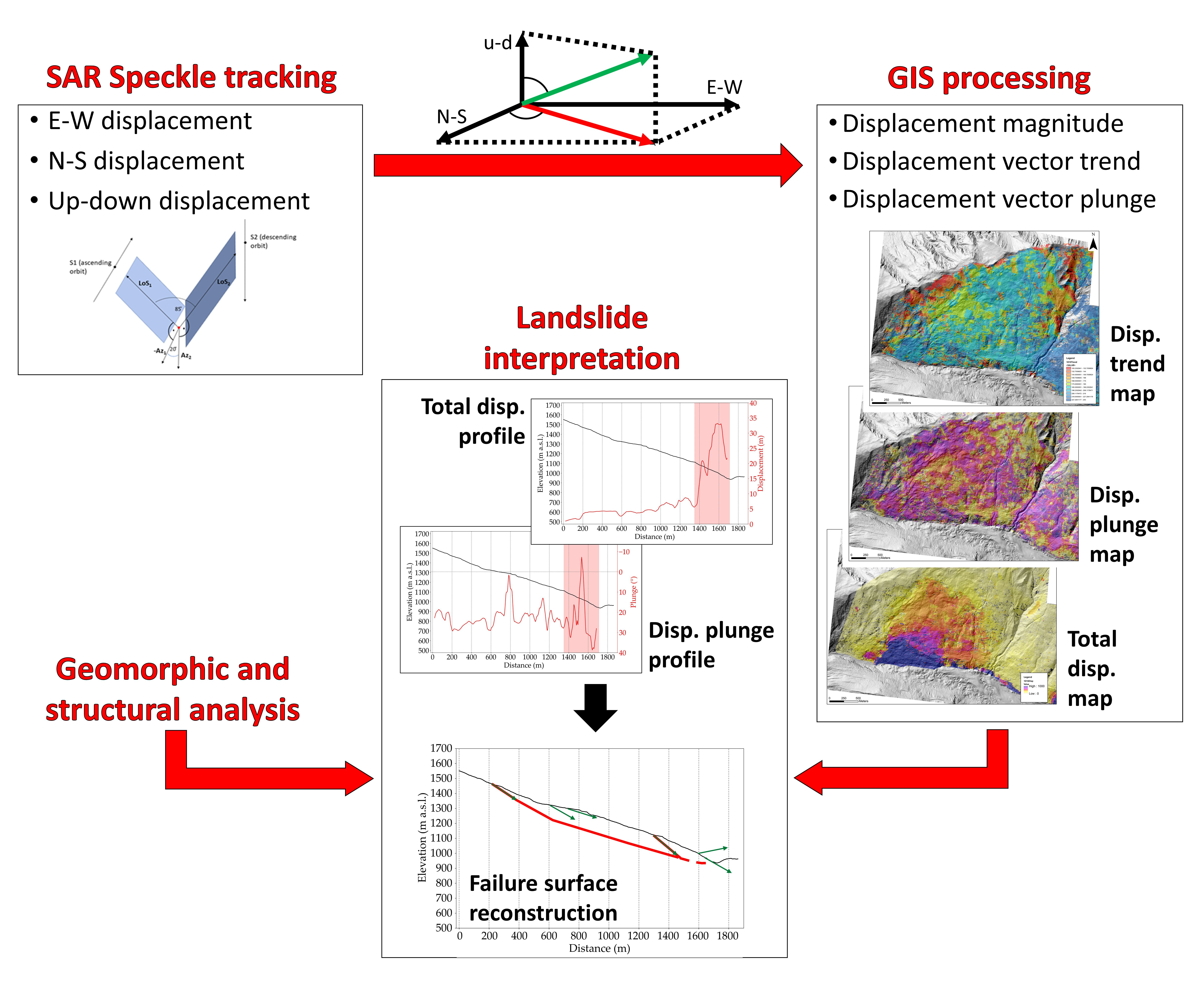
Fels landslide is located in the Alaska Range about 150 km southeast of Fairbanks, on the north slope of Fels Glacier valley, which is a tributary of the Delta River valley (
Figure 1). The Delta River valley contains two important infrastructure elements, the Trans-Alaska Pipeline and the Richardson Highway. Fels Glacier terminates at an elevation of 820 m a.s.l., about 3 km from the pipeline and highway (
Figure 1a). The glacier has been retreating for more than a century, since the end of the Little Ice Age. A comparison of aerial photographs taken in 1949 and 2017 shows that the glacier retreated more than 900 m over this period. Within Fels Glacier valley, slope deformation involves two areas, referred to as “lobe a” and “lobe b”, that are divided by a deeply incised gully, perpendicular to the valley [
45]. Lobe a displays significantly higher deformation rates and prominent slope damage features, compared to lobe b (
Figure 1a). In this paper, we consider lobe a as the Fels landslide, and we primarily focus our analysis on this part of the slope.
Fels landslide has a surface area of about 2.3 km2 and extends 1400 m in the E–W direction and 1600 m in the N–S direction between elevations of 920 and 1490 m a.s.l. The ground surface within the landslide area has an overall slope of 20–30° to the S, steepening up to a slope angle of 40–50° at its glacially eroded toe.
Bedrock in the landslide area comprises fine-grained Devonian metasedimentary rocks of the Jarvis Creek Glacier subterrane, mainly quartz-mica schist and quartzite, with lesser chlorite-muscovite schist, quartz-biotite schist, calc-schist, and marble [
46,
47]. The rock mass has a prominent slope-parallel foliation (D1 in
Figure 1b), and two other orthogonal discontinuity sets (D2 and D3 in
Figure 1b). Much of the slope surface is covered by colluvium that hosts localized surficial slumps (
Figure 1c). Glacial deposits, including till and outwash are associated with lateral and frontal moraines in the lower part of Fels valley and in the Delta River valley [
46].
The active, dextral Denali Fault is located 3 km south of the Fels landslide (
Figure 1a). It strikes NW–SE and follows and controls the orientation of the Canwell valley, which neighbors Fels valley on the south. The dip of the regional foliation increases toward the fault, from 20–25° in the area of the Fels landslide to 50–60° in Canwell valley [
46]. An M
w 7.9 earthquake occurred on the Denali Fault on 3 November 2002. Many co-seismic rock avalanches, rockslides, slumps, and debris avalanches were triggered by the earthquake in the epicentral area [
45]. Although no major landslides occurred within Fels valley, the intense ground shaking, exacerbated by material and topographic amplification [
48], is likely to have enhanced internal damage (e.g., rock mass dilation, fracture propagation) within the slope [
45].
Historical, geological, and geomechanical analyses that we performed and will be presented in detail in another paper indicate that the current instability phase in the Fels Glacier valley was initiated by glacier retreat, which provided kinematic freedom for movement of the toe of the landslide. Slumping at the toe, in turn, caused the instability to propagate upslope, where displacements are occurring by planar sliding along a slope-parallel rupture surface that is likely controlled by foliation.
3. Description of the New Method and Application to the Fels Landslide
3.1. Overview of the Proposed Methodology
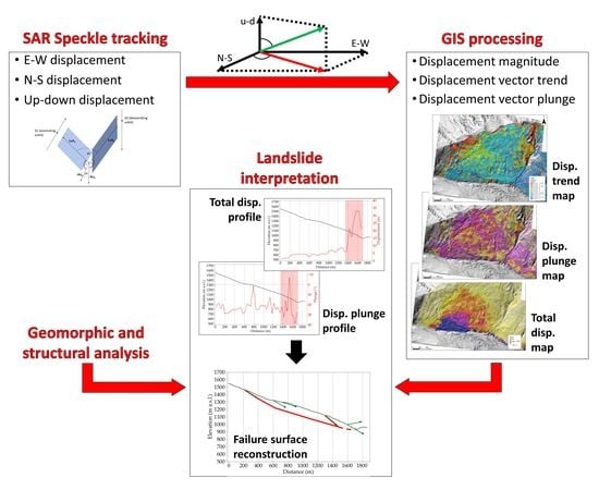
Figure 2 schematically summarizes the proposed methodology; subsequent subsections describe in detail each step for the Fels landslide example. The workflow to determine 3D vectors of surface displacement comprises three steps. Step 1 is SAR speckle tracking data processing. Input SAR image data for this step were acquired from both ascending and descending orbit look directions at the boundaries of the two subsequent 5-year intervals of the period 2010 and 2020 using RADARSAT-2′s high-resolution spotlight mode. From tracking temporal shifts between images, we were able to determine the 3D composition of the displacement field. The ST and subsequent vector decomposition algorithms produce the total displacement components in the horizontal (E–W, N–S) and vertical (up–down) directions. Step 2 involves GIS raster processing and produces the local magnitude, plunge, and trend of the 3D displacement vectors from the components calculated in the first step. Step 3 is the creation, within a GIS environment, of thematic maps (hillshade, vector orientation and magnitude, and lineaments and lineament distribution). Cumulative displacement and displacement plunge profiles were extracted from the step 3 datasets and compared to elevation profiles, allowing us to examine the effects of slope deformation on the ground surface. Analysis of the datasets over time (i.e., comparing the two 5-year periods) provides a preliminary assessment of the style of deformation, setting the stage for targeted field and subsurface analyses.
3.2. Speckle Tracking (ST) Processing
For each orbit (ascending and descending) geometry separately, we first carry out a precise global registration of the primary high spatial resolution SAR data pairs acquired at the start and end of the observation period. The chosen registration algorithm resamples the geometry of the later image to match that of the earlier image using a low-order, two-dimensional polynomial. Further the process masks out the landslide area where we expect movement, so that the two-dimensional polynomial registration accurately maps the stationary areas around the landslide to better than one tenth of the full resolution pixel dimensions.
Next, we find local fine-registration offsets for the already globally registered image pairs using spatial correlation measurements on a dense regular raster grid of small rectangular image chip pairs. We are sinc-oversampling both images by factor four before extracting the chips and then using normalized cross-correlation of the detected chip amplitudes for the actual offset measurements. Our approach tracks the displacement of both coherent speckle patterns and macroscopic features at the same time, in contrast to complex coherence optimization, which only tracks coherent speckle patterns. The result is a corresponding raster grid of local offsets in the radar geometry, in range line of sight (LoS), and in satellite orbit direction, called azimuth (Az). To maximize spatial resolution of the local offset map, we chose rectangular image chips as small as possible to allow accurate offset determination using normalized cross-correlation measurements. By doing so we maximize resolution in the presence of both random macroscopic changes unrelated to the large-scale landslide displacement (e.g., displaced individual blocks or newly formed cracks) and incoherent parts of the image speckle pattern caused by sub-resolution changes of the surface between the earlier and later date (e.g., due to vegetation or snow patches).
In our case study, the primary SAR images are RADARSAT-2 Spotlight mode with a resolution of about 1.3 m in LoS and 0.4 m in the satellite flight direction (Az). Consequently, we chose a rectangular chip size of 51 by 255 pixels in, respectively, range and azimuth, corresponding to an approximate ground distance of ~95 by ~102 m (mean incidence angle 44°) for the resulting local offset map. We chose the grid density to be half the chip size (47 by 51 m). Choosing the raster grid of the resulting offset maps finer than the chip size creates spatial redundancy that allows us to filter out and smooth errors from erroneous local correlation matches. Increasing the raster grid size, however, lengthens the runtime of the numerically expensive correlation measurements. The chosen raster grid spacing is a reasonable compromise between redundancy/robustness and runtime.
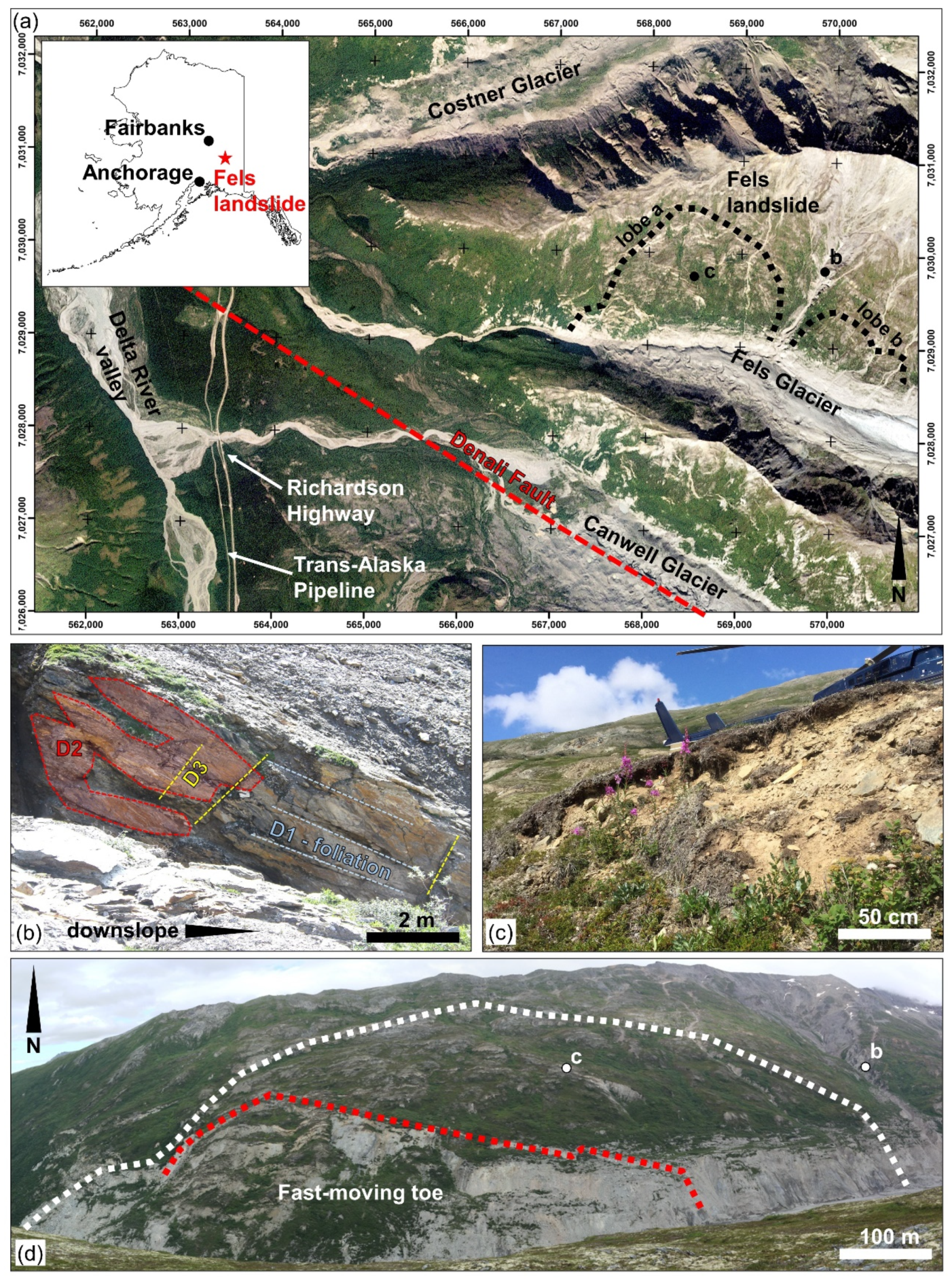
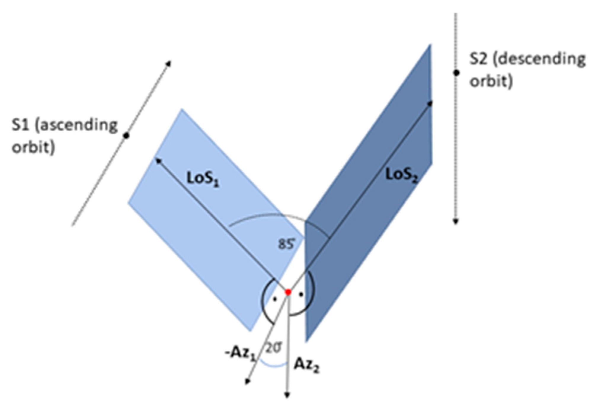
The resulting offset maps from multiple radar geometries, each consisting of a pair of LoS and Az measurements in the respective geometry, we then geocode from radar to map geometry using an external high-resolution DSM (digital surface model). Next, we carry out a vector inversion of these now spatially matching offset maps to determine the 3D surface displacement vector components. Multiple geometries for InSAR consisting exclusively of LoS measurements require more than two acquisitions to invert 3D movement from the measurements without additional assumptions. Due to unfavorable LoS geometries the inversion quality is generally quite poor for InSAR, leading to large errors in the 3D vector components. However, the opposite is true for inverting multiple ST geometries consisting of both LoS and Az offset measurements. As
Figure 3 shows, just two ST geometries, one from an ascending orbit and another from a descending orbit, which provide measurements LoS1, Az1, LoS2, and Az2, are sufficient to invert 3D geometry without additional assumptions. The resulting inversion quality is high, and thus projection errors of the 3D-vector components are reasonable.
We use a standard least square inversion technique [
49] to solve for the 3D vector components. We build a 3 × 3 design matrix from multiplying with its transpose the 3 × 4 input matrix formed by the four offset measurement LoS1, Az1, LoS2, and Az2 corresponding to the known satellite orbit geometries. The design matrix is then inverted to arrive at the easting, northing, and up components of the displacement. Az is measured parallel to the orbit, and LoS for most SAR sensors can be assumed to be measured perpendicular to the orbit. As will be described in the following step, the “global” 3D vector components, easting, northing, and up, can be easily converted a posteriori to another global system: plunge, trend, and magnitude. Alternatively, one could also convert to an adaptive “local” system of fall line, contour, and emergence (local surface normal) components by using an external, high-resolution DSM.
For the analysis of the Fels landslide example, we used a total of six RADARSAT-2 scenes captured in Spotlight mode (
Table 1 and
Figure 4). The periods of the scene pairs for the ascending and descending orbit geometries differ by just one day, which provides near-ideal conditions of temporal coincidence of the offset measurements for the vector component inversion. Scenes were captured roughly five years apart, spanning the period between 14 July 2010 and 3 August 2020.
3.3. GIS Post-Processing
The raster displaying the E–W, N–S, and vertical components of the deformation vectors are imported in a GIS environment to derive the trend, plunge, and magnitude of displacement. The datasets described in this section were derived using the “calculate raster” tool available in the software ArcGIS 10.6 [
50].
The total horizontal (D
H) and 3D (D
3D) magnitude of the displacement vector are first computed as
respectively, where D
EW, D
NS, and D
V are the three components of the deformation vector obtained from the ST analysis in the previous step.
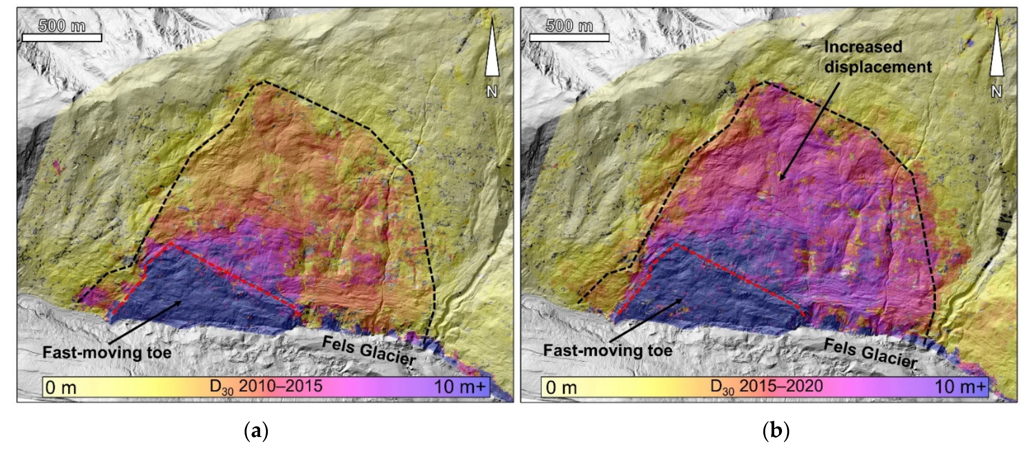
Figure 5 shows the resulting raster datasets for the investigated time windows, 2010–2015 and 2015–2020, from which the high deformation magnitude in the fast-moving slope toe (up to 30 m) can be observed. In the 2010–2015 time window, displacement magnitudes decrease spatially to about 10 m in the area immediately upslope of the fast-moving toe, and then progressively to about 2 to 3 m in the upper slope. In the 2015–2020 window, a similar decreasing trend is observed, but the computed displacement magnitudes are higher across the entire landslide area.
The trend of displacement, θ, is then computed using the N–S component of the displacement vector and the previously computed D
H. First, the angle
is calculated. This α-angle is then used to compute the displacement trend, based on the quadrant (I-IV) where the displacement vector plots (i.e., depending on the sign of the N–S and E–W components).
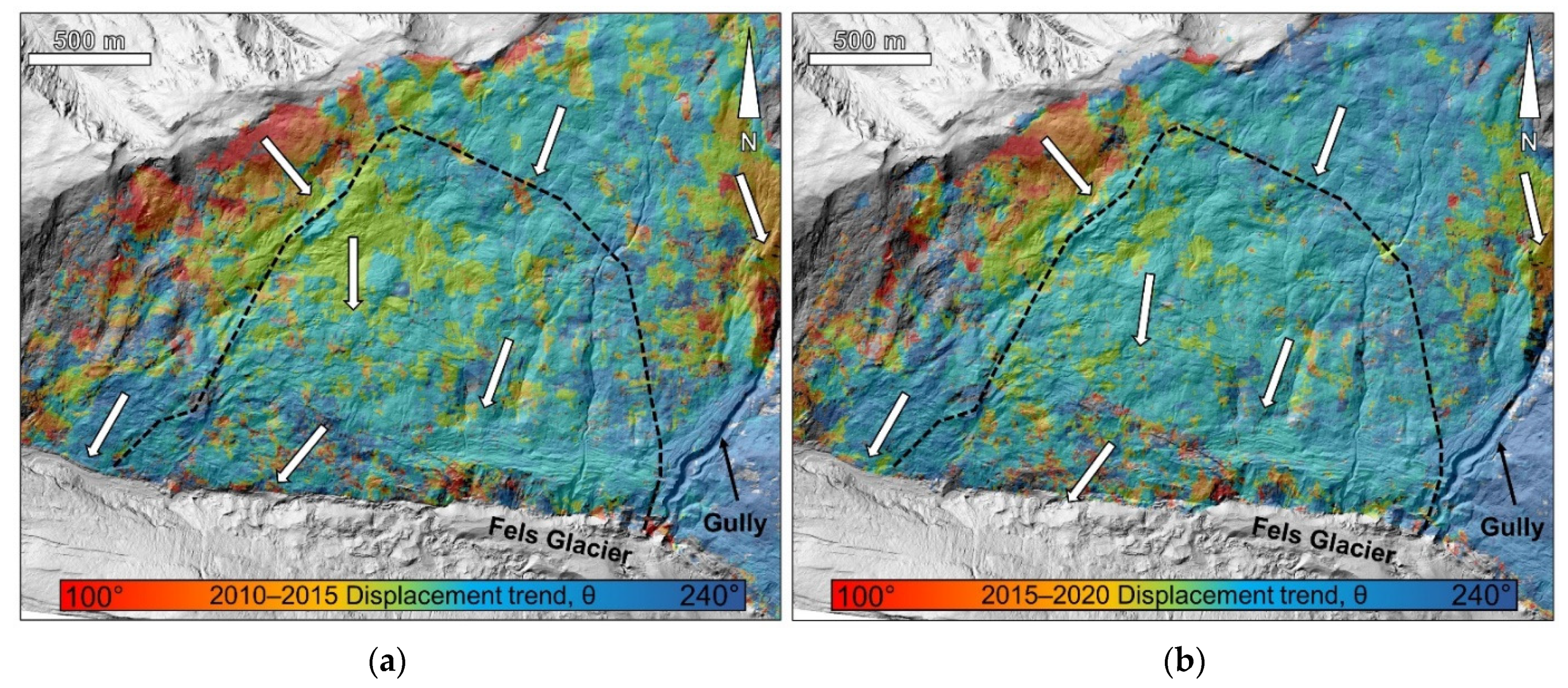
The raster dataset of the trend of displacement is shown in
Figure 6. As the slope is predominantly deforming in a southern direction, the color scale is adjusted to highlight corresponding trend values between 100° and 240°.
The angular deviation of the displacement vector from the horizontal is referred to as the plunge of displacement. Its characterization and analysis allow the style of deformation and, potentially, the failure mechanism to be inferred. Characterizing the plunge of displacement is important for the interpretation of active landslides using ST datasets. The plunge of deformation, ψ, is computed using the vertical displacement value, D
V, obtained from the ST analysis, and the total displacement D
3D:
The sign of ψ is defined by D
V. Positive and negative values of D
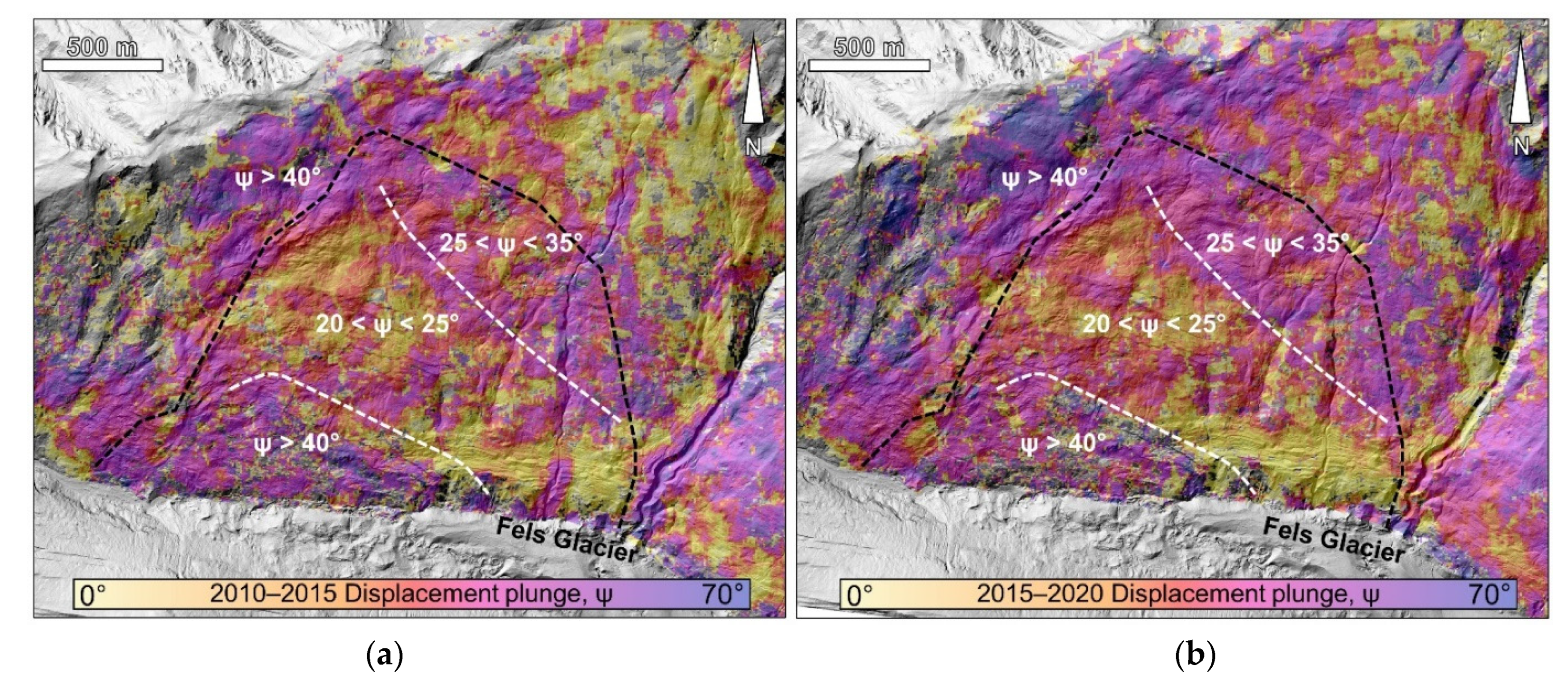
V result in, respectively, negative and positive values of ψ, indicating, in turn, upward and downward displacements. The resulting raster dataset, displayed in
Figure 7, shows that high positive plunge values occur in the lower part of the slope, corresponding to the fast-moving toe of the landslide. Lower downward plunge angles, between 20 and 25°, are found in the central part of the slide area. The upper part of the slope displays plunge angles between 25 and 35°, indicating steeper downward deformation compared to the central part. Minor changes in displacement plunge distribution can be noted between the 2010–2015 (
Figure 7a) and 2015–2020 periods (
Figure 7b), but a similar pattern is evident in both datasets.
3.4. Integrated Analysis of Remote Sensing Data
The value of high-resolution remote sensing datasets, such as ALS, for structural and geomorphic characterization of rock slopes has been demonstrated by several authors [
51,
52,
53]. In this section, we document the implementation of ST analyses in a comprehensive workflow for the characterization of rock slope instabilities, providing insights on their style of deformation and failure mechanism.
3.4.1. Profile Extraction and Analysis
The 2.5D nature (i.e., a 2D grid in which each cell is assigned a scalar value, producing a pseudo-3D geometry) of the ST datasets allows profiles to be extracted and compared with elevation data obtained from the ALS model. The combined analysis of plunge, displacement, and elevation profiles facilitates identification of geomorphic features produced by slope deformation (e.g., uphill- and downhill-facing scarps, grabens, slope breaks).
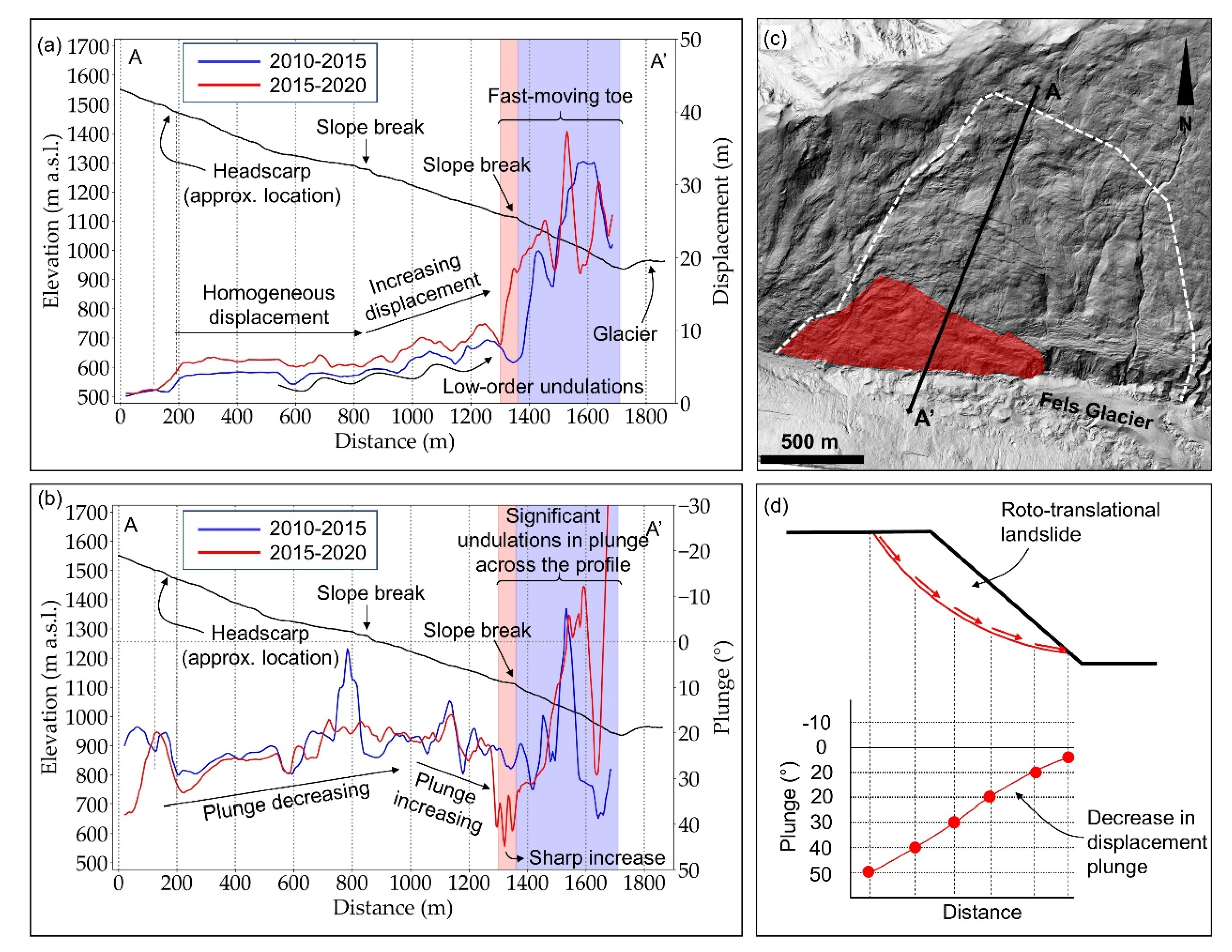
Figure 8a,b shows displacement magnitude and plunge values for the 2010–2015 and 2015–2020 time windows along a profile parallel to the displacement direction (
Figure 8c). The displacement profiles display a constant magnitude in the upper slope, suggesting that the landslide body is deforming as a single block. A progressive downslope increase in displacement magnitude begins at about 1300 m a.s.l. in the central part of the slope and continues downward to the boundary with the fast-moving slope toe at 1100 m a.s.l. Low-order undulations are evident within this zone, which locally cause the cumulative displacement to decrease downslope (
Figure 8a). These undulations may be caused by shallow secondary instability (e.g., soil slumps) within the colluvial deposit blanketing the slope (
Figure 8c). The transition between the uniformly displacing part of the slope and the part with an increase in displacement roughly coincides with a break in the elevation profile where the slope steepens. A slope break also marks the upper boundary of the fast-moving toe.
This complex pattern in displacement magnitude is in accord with the deformation plunge profile (
Figure 8b). Undulations in amplitude (up to 15–20°) are observed along the profile, and particularly between elevations of 1300 and 1100 m a.s.l. These undulations are superimposed on the larger scale trend of the profile, which shows an overall decrease in plunge in the upper slope, between the headscarp and the slope break at 1300 m a.s.l., followed by an increase in plunge in the central and lower slope. The area of increased plunge roughly corresponds to the increase in displacement magnitude in the central part of the slope. The decrease in plunge in part of the profile lower on the slope corresponds to the fast-moving toe, where significant undulations in plunge occur.
The displacement magnitude and plunge profiles extracted from the 2010–2015 and 2015–2020 ST datasets have similar patterns. However, the displacement magnitude profile for the 2015–2020 time window is consistently higher than for the 2010–2015 dataset, indicating that the displacement that occurred between 2015 and 2020 exceeded the displacement between 2010 and 2015. Additionally, the sharp increase in displacement magnitude in the lower slope, marking the boundary of the fast-moving toe, occurs roughly 50 m farther upslope in the 2015–2020 dataset compared to the 2010–2015 dataset (blue and red bars in
Figure 8a,b). Similarly, a sharp increase in displacement plunge is evident in the 2015–2020 profile, indicating a stronger downward component of the deformation vector along the upper boundary of the fast-moving toe compared to the 2010–2015 profile.
3.4.2. Correlations between Structural Lineaments and ST Datasets
We compare the magnitude and distribution of the surface displacements computed from the ST analysis with the location, distribution, and orientation of lineaments identified and mapped from the ALS dataset. A summary of the lineament mapping is provided here, to demonstrate the advantages of an integrated ST-ALS analytical approach.
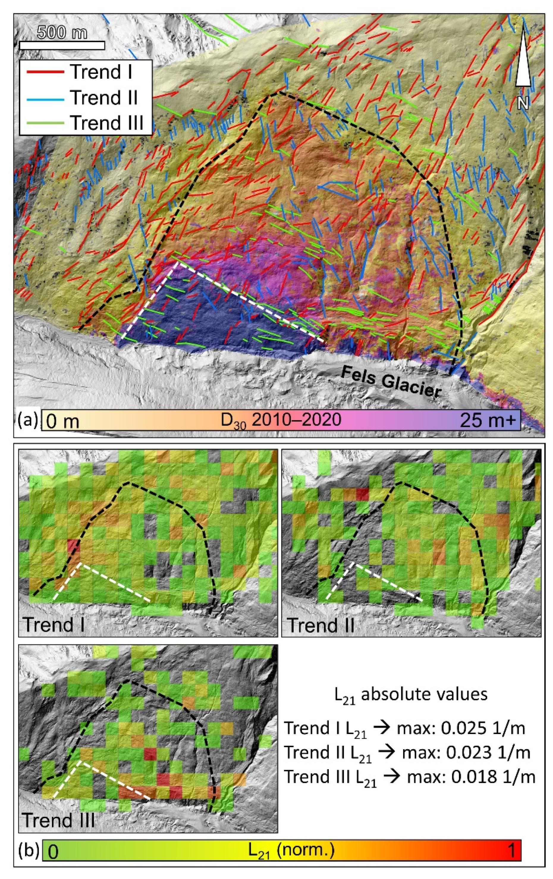
We identified three different lineament trends, I, II, and III, at Fels landslide using the ASL dataset. They are oriented NE–SW, NNW–SSE, and NW–SE, respectively (
Figure 9a). The spatial distribution of the lineaments was also investigated in terms of lineament intensity (L
21), defined as the ratio of the total length of lineaments to the sampling area and measured in 1/m. We note higher L
21 values for trend I in the western part of the slope. Trend II displays high L
21 values in the central and lower parts of the slope within and upslope of the fast-moving toe and, locally, in the upper slope. We note high L
21 values for trend III outside the western boundary of the slide and in the central-eastern part of the slide area (
Figure 9b).
Comparison of the lineament and displacement magnitude maps shows significant correlation between the datasets. The boundaries of the landslide area can be roughly approximated by straight lines, with orientations similar to the identified lineament trends. The western boundary of Fels landslide is parallel to lineament trend I, and its location corresponds to the part of slope where the same trend has a high L21. The orientation of the eastern and upper boundaries of the landslide area are sub-parallel with trend II and trend III lineaments, respectively. The fast-moving toe appears to be outlined by scarps parallel to trend I on the west side and trend III along the rear boundary. We conclude that the landslide is structurally controlled and that the surface deformation obtained from the ST analysis is mainly related to displacements originating at depth within the bedrock, rather than within the colluvial blanket draping the slope.
3.4.3. Reconstruction of the Sliding Surface and Estimation of Landslide Thickness
The plunge and trend of displacement of a landslide that moves as a rigid or stiff block, or a combination of blocks, are related to the morphology of the sliding surface [
8]. The spatial analysis of displacement plunge, ψ, across the landslide area therefore provides insight into the deformation style and failure mechanism of a landslide.
The location and morphology of a sliding surface can be inferred from the distribution and magnitude of surface displacement both vertically and horizontally. The simplest method, referred to as the vector inclination method (VIM), assumes that the trend and plunge of displacements reflect the local orientation of the sliding surface [
54,
55], which with this method can then be graphically reconstructed along user-defined sections. The development of remote sensing techniques, such as InSAR and ALS, capable of monitoring wide ground surface areas allows researchers to use the VIM method to quickly estimate the thickness of active rock slides [
56]. A more advanced approach exploits the mass conservation equation to estimate differences in depth of the sliding surface over large areas. This approach, originally developed to infer the thickness of glacier ice [
57], was later adapted to the investigation of rock slope instabilities [
58,
59].
We estimate the thickness of Fels landslide using the VIM method because it is relatively simple and easy to apply, and in order to enhance comparison with the ST profiles shown in
Figure 8. Use of the VIM method involves two significant assumptions about the characteristics of the slope instability. The first is that the landslide displacement can be approximated with that of a rigid body; therefore the method is not suited for the investigation of flow-like landslides. Based on the distribution of computed displacements (
Figure 5), and the structurally controlled nature of the instability inferred from the lineament mapping, Fels landslide can be preliminarily approximated as a rigid body, as the measured displacements have similar magnitude and orientation across the surface area of the landslide, except at the fast-moving toe. The second assumption is that the landslide displaces along a single discrete sliding surface. Soil slumps occur at Fels landslide in the blanketing colluvial material, entailing the local presence of multiple sliding surfaces (i.e., the sliding surface at depth, and the shallow sliding surfaces of the soil slumps). However, small-scale undulations can be filtered from the plunge profile (
Figure 8b) by selecting for the VIM reconstruction only those plunge values that correlate with negative peaks in the cumulative displacement profile (
Figure 8a). The rationale for this approach is that areas with surface slumping will display higher displacement magnitudes than areas with no slumping, where cumulative displacement is only, or predominantly, due to sliding at depth. Therefore, negative peaks in the displacement profile are more likely to represent locations within the slide area that are less affected by surface slumping. In turn, the associated plunge values will be primarily controlled by the sliding surface at depth.
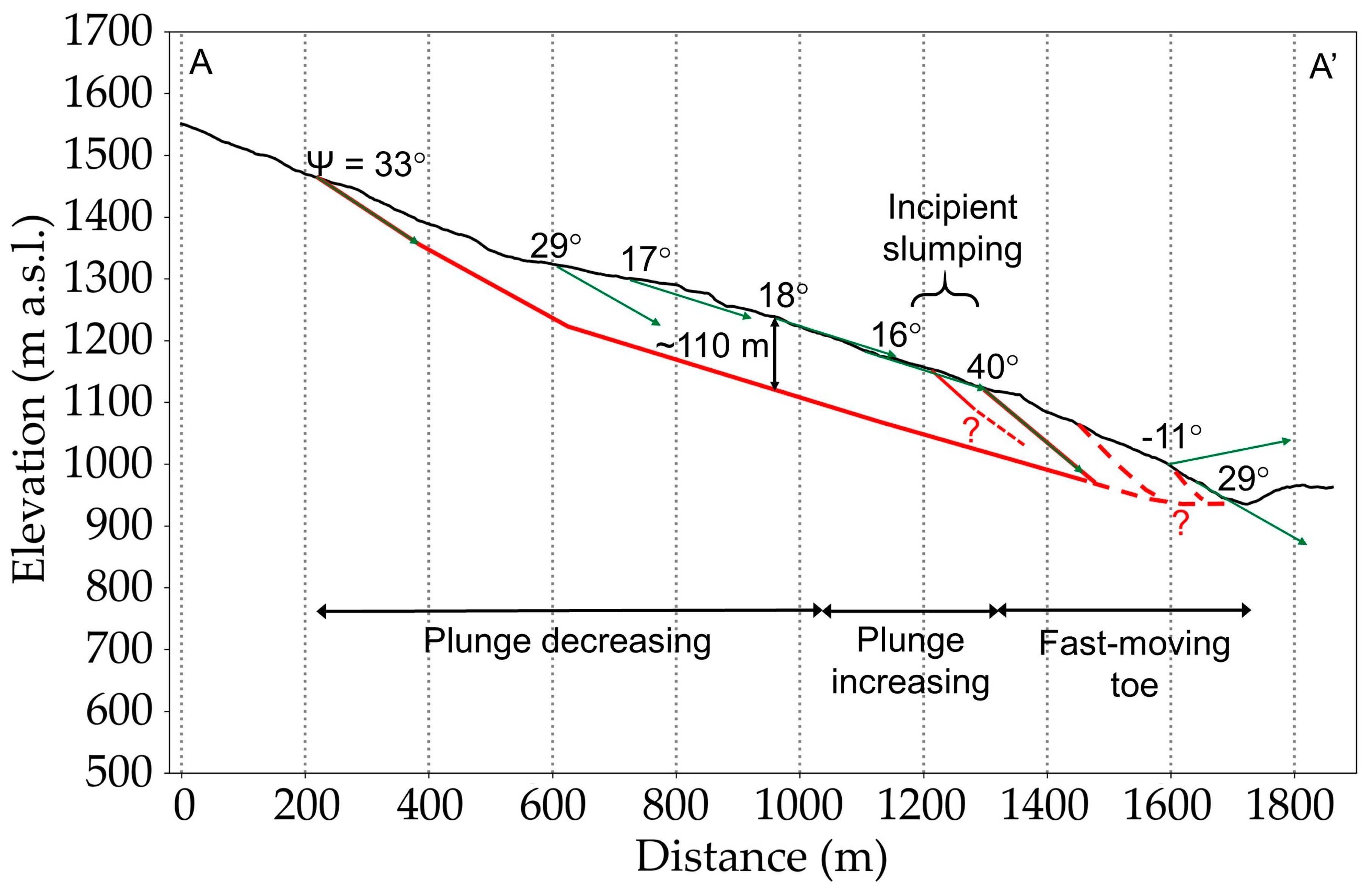
We reconstructed a section of the sliding surface along the A-A’ profile (
Figure 10) and estimated a maximum thickness of about 110 m for the landslide along this profile. The reconstructed rupture surface displays a relatively high angle at the headscarp (33°), progressively decreasing to about 17° in the mid-slope position. The fast-moving toe is marked by a sharp increase in plunge (40°), which identifies the upper boundary of the slumping instability observed in the field (
Figure 1d).
4. Discussion
The combined ST-ALS approach proposed in this paper allows for a preliminary interpretation of the failure mechanism of a large, slow-moving landslide (Fels landslide) using remotely sensed data. Based on the spatial distribution of the displacement magnitude and plunge, as well as the evolution of these two components with time, we found that the Fels landslide accelerated between 2010 and 2020. Due to the limited temporal resolution of the ST datasets, however, the factors that drove this increase in displacement remain unclear.
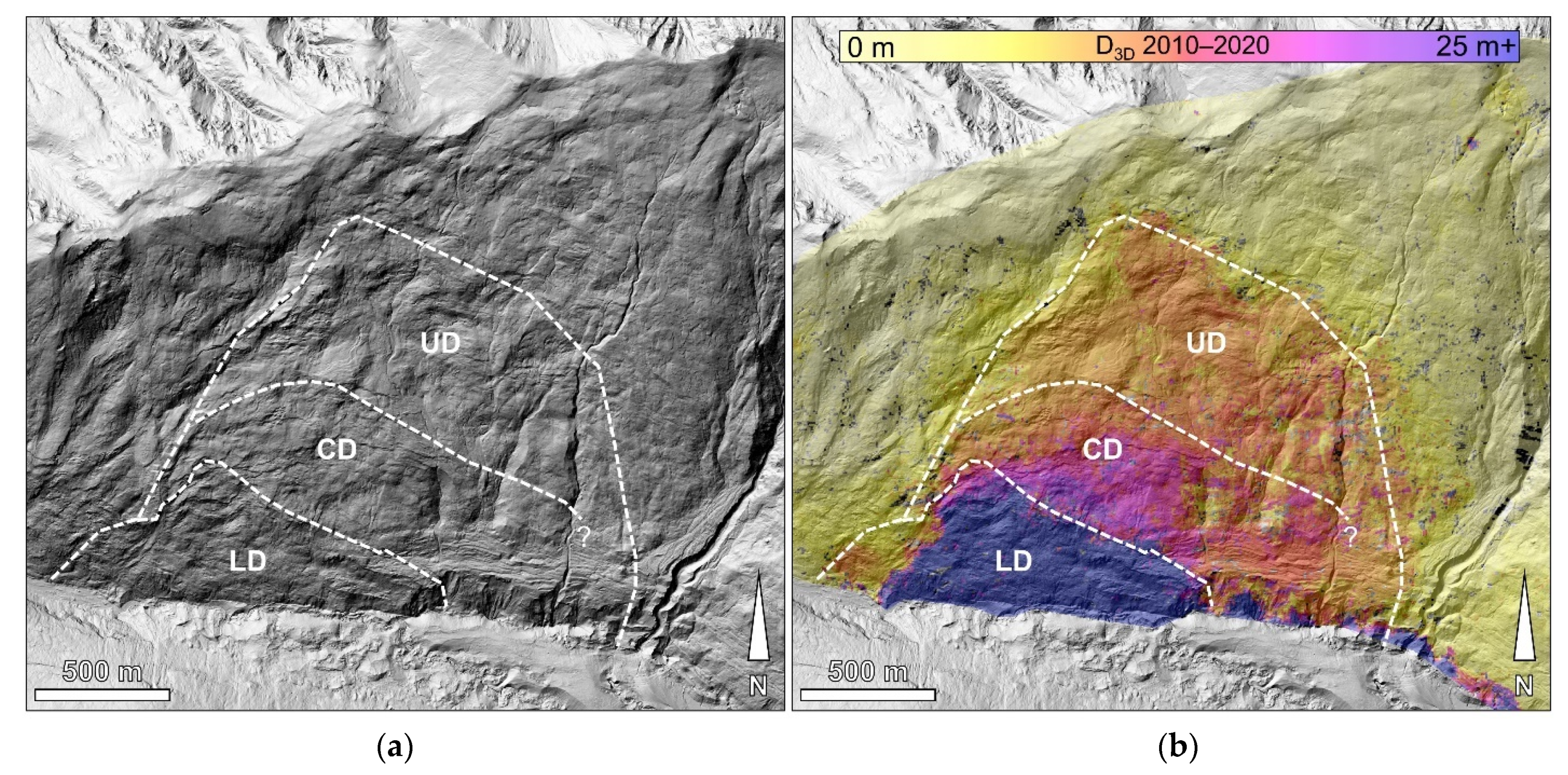
Based on our ST results, the reconstructed sliding surface, and the visual observation of the slope and ALS dataset, we propose a subdivision of the Fels landslide into three different domains: upper, central, and lower (
Figure 11).
The upper domain is a slowly moving block with displacement rates of up to 1 m/year. Here, slope-parallel deformation vectors suggest that the displacement is occurring along a sub-planar sliding surface, likely controlled by foliation, that connects with the ground surface in the upper part of the domain (i.e., daylights). The headscarp does not correlate with any prominent geomorphic feature, suggesting that displacements noted in the upper slope are relatively recent, and colluvial material may be smoothing the ground surface. The style of deformation of the upper domain remained unchanged between 2010 and 2020.
The central domain is characterized by displacement rates ranging from 1 to 2 m/year, with a progressive increase in the downslope direction. A progressive increase in plunge is also noted across the domain, with the highest values (nearing 35°) observed toward the fast-moving toe (
Figure 8b), indicating steepening and lengthening of the displacement vectors. We note a significant increase in displacement magnitude during the 2015–2020 time window (
Figure 8a).
The lower domain is the fast-moving toe that appears to be displacing by a rotational (slumping) or pseudo-rotational mechanism (i.e., characterized by a spoon-shaped sliding surface), with displacement rates up to 5–8 m/year over the 2010–2020 period.
The central domain appears to be transitional in nature between the lower, fast-moving domain and the upper, slow-moving domain. The observed increase in plunge is likely not related to a steepening of the sliding surface, but rather to a local progressive change in failure mechanism from planar sliding to a pseudo-rotational mechanism (
Figure 10). The transition between planar sliding and slumping is also evident from the changes in the displacement plunge profile at the boundary between the central domain and the fast-moving toe, between the 2010–2015 and 2015–2020 periods. The increase in displacement plunge shows that the volume upslope of the fast-moving toe was displacing through a planar sliding mechanism between 2010 and 2015, before transitioning to pseudo-rotational mechanism between 2015 and 2020.
We suggest that Fels landslide is characterized by a bi-planar or multi-planar configuration. The landslide section reconstructed in
Figure 10 shows that the sliding surface is sub-parallel with the slope surface in the central part of the landslide. There must be a decrease in the dip angle of the sliding surface, therefore, in order for the basal surface to daylight below the fast-moving toe. Such a change in dip angle may result from (a) a local change in the orientation of the foliation within the lower slope, or (b) the accumulation of internal rock slope damage (i.e., a combination of rock mass yielding, dilation, and intact rock fracturing) due to gravitational displacement and stress concentration. The colluvial material blanketing the toe of the slope precludes any observation of the orientation of the foliation orientation. However, regional data presented in [
46] shows that the dip angle of foliation generally increases toward the south (i.e., approaching the Denali Fault), suggesting that a structural geology origin at the toe can be ruled out. Therefore, we suggest that such a bi-planar configuration is likely related to a combination of gravitational and glacial processes.
5. Conclusions
The workflow presented in this paper combines ST and ALS techniques to enhance the interpretation of deformation and failure mechanisms of unstable rock slopes. The application of this combined method in the investigation of Fels landslide allowed us to recognize the structural geologic control on the slope deformation and to infer the failure mechanism and its evolution based on surface deformation and geomorphic data.
The proposed approach can be further expanded through the inclusion of datasets derived from other aerial and ground-based sensors (e.g., thermal and hyperspectral imagery, high-resolution photography), to provide information on locations of groundwater seepage, slope constitutive material and rock type, and the possible presence of localized material alteration.
From a monitoring perspective, the benefits of our proposed approach are significant. Advantages of ST analysis over traditional SAR-based monitoring techniques include: (a) its capability of providing (robustly with small error brackets and from just two geometries, one ascending and one descending) the true 3D displacement vector; not only in the E–W and vertical directions, but also in the N–S direction that traditional InSAR is notoriously insensitive to, and further (b) the ability to monitor slopes that deform at higher rates of several meters per year. On the flip side, ST analyses with sufficient spatial resolution rely on primary SAR data with very high resolution and interrogate slope deformation over relatively long periods compared to more sensitive techniques such as InSAR. This potentially will obscure or mask effects of high-frequency or seasonal events and single processes such as snowmelt, rainfall, and earthquakes. Additionally, the application of the ST technique may be limited in areas with low coherence, such as heavily vegetated areas, or where changes in land cover occur during the investigated time window. The proposed approach including ST can potentially provide an effective long-term monitoring strategy for large, slow-moving landslides. A preliminary analysis that takes advantage of the proposed approach can also be beneficial for planning field activity, geophysical surveys, borehole drilling, as well as in the development of an in situ monitoring system (e.g., location and depth of borehole inclinometers).
In this paper, we have demonstrated that the use of multiple remote sensing data, combined with advanced processing and post-processing techniques, can contribute to composite datasets that are instrumental for the investigation of slow-moving landslides. Integrating slope-scale interpretations with outcrop scale, rock mass characterization, however, is important for identifying the possible role of smaller discontinuity sets, rock mass quality, and intact rock strength on the deformation of the rock slope. The collection of such data cannot rely solely on remote sensing techniques, which are non-contact in nature and do not allow the mechanical properties of the materials to be inferred. Therefore, traditional, field-based assessments are critical to validate the interpretation made from remote sensing analyses and remain a fundamental step for comprehensive rock slope characterization.


 ,
, 


