
A Method for Quantifying Understory Leaf Area Index in a Temperate Forest through Combining Small Footprint Full-Waveform and Point Cloud LiDAR Data


Abstract
:1. Introduction
2. Materials
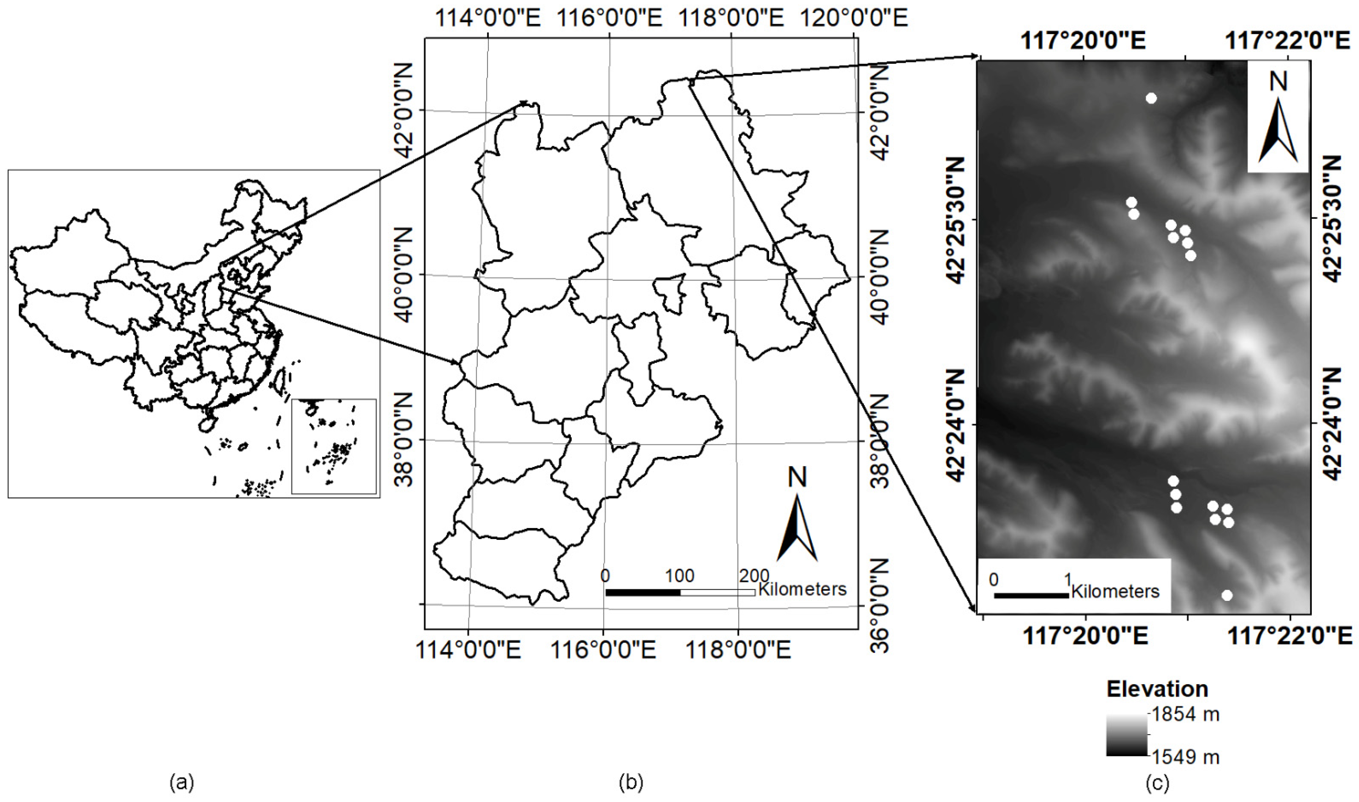
2.1. Study Area and Field Data
2.2. LiDAR Data
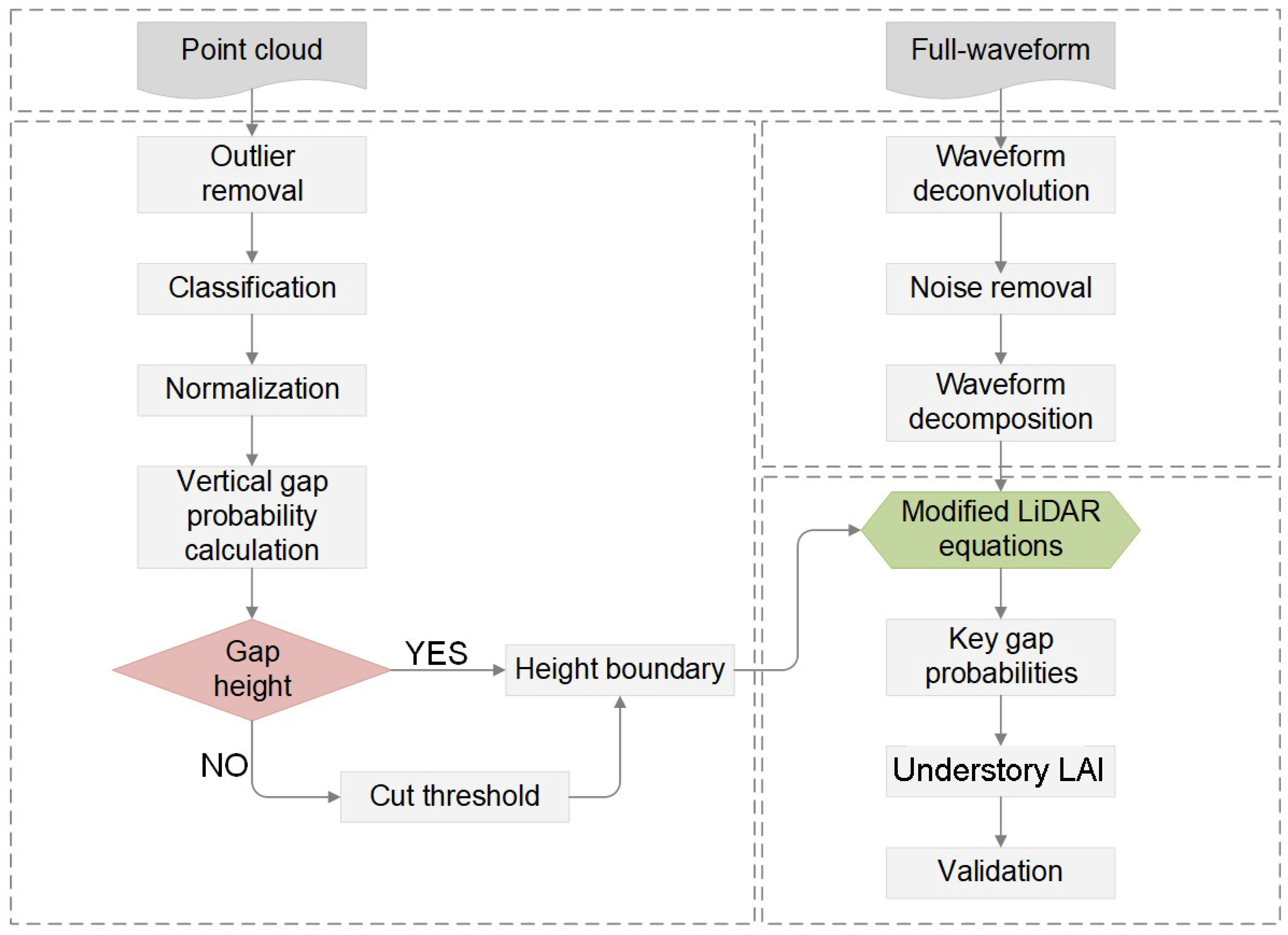
3. Methods
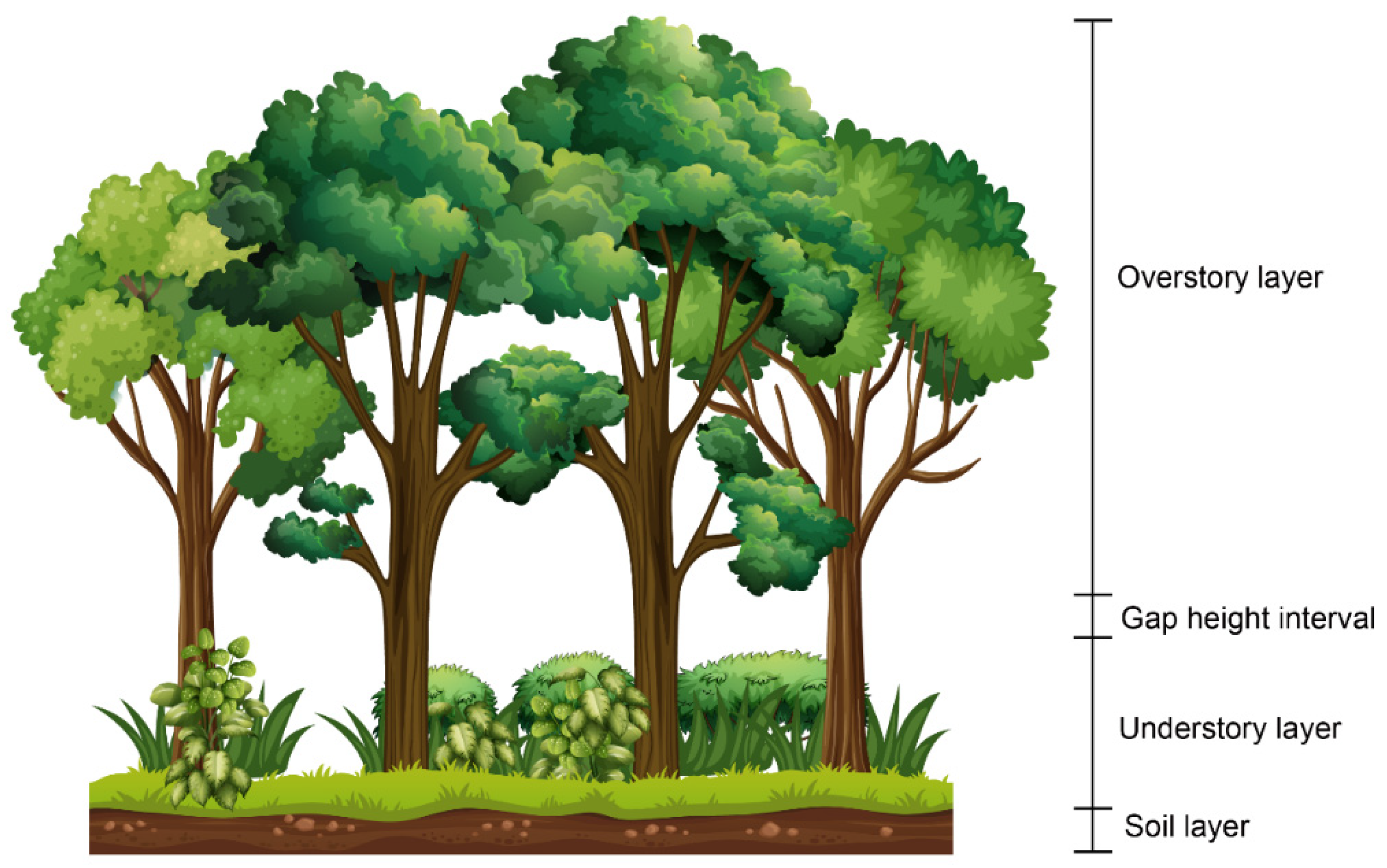
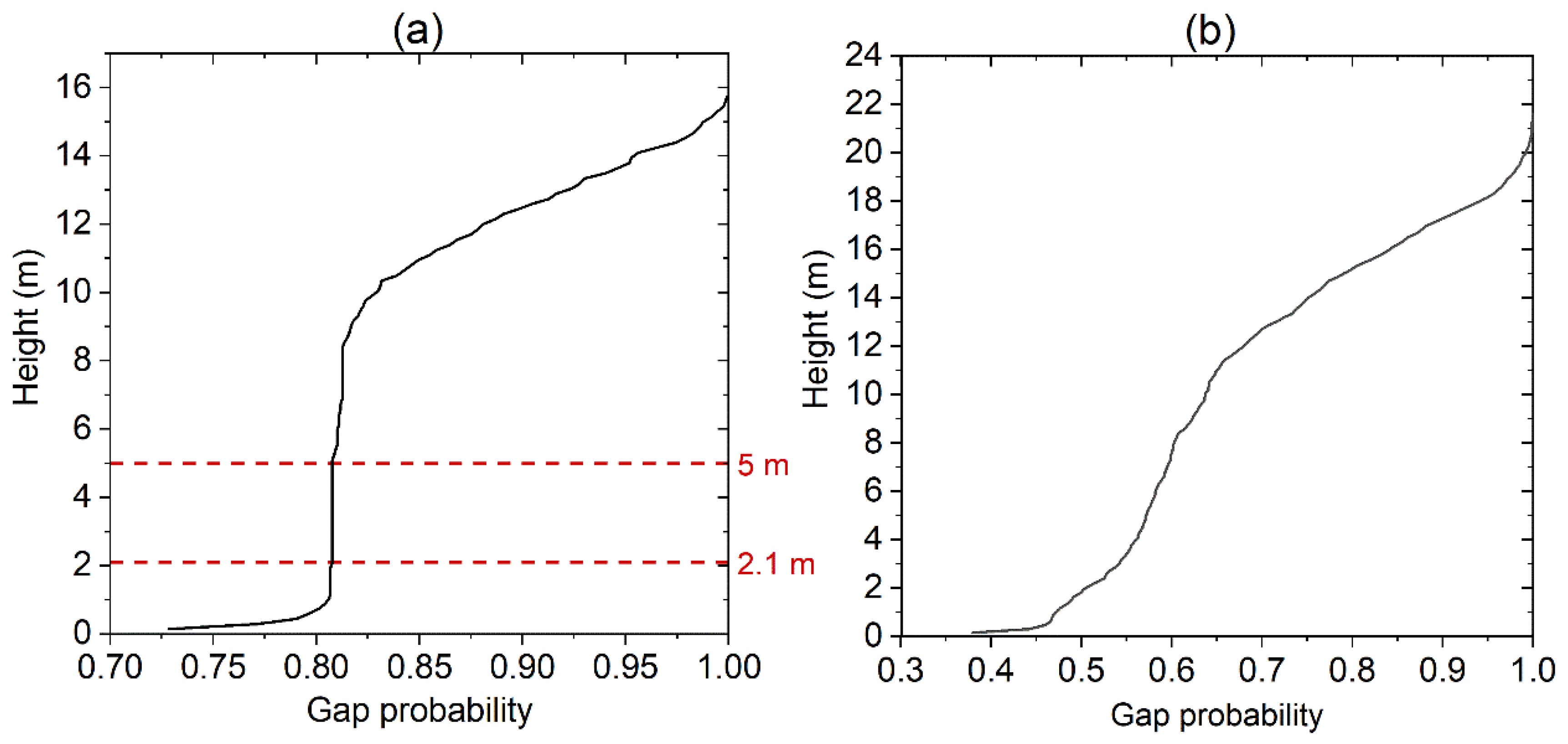
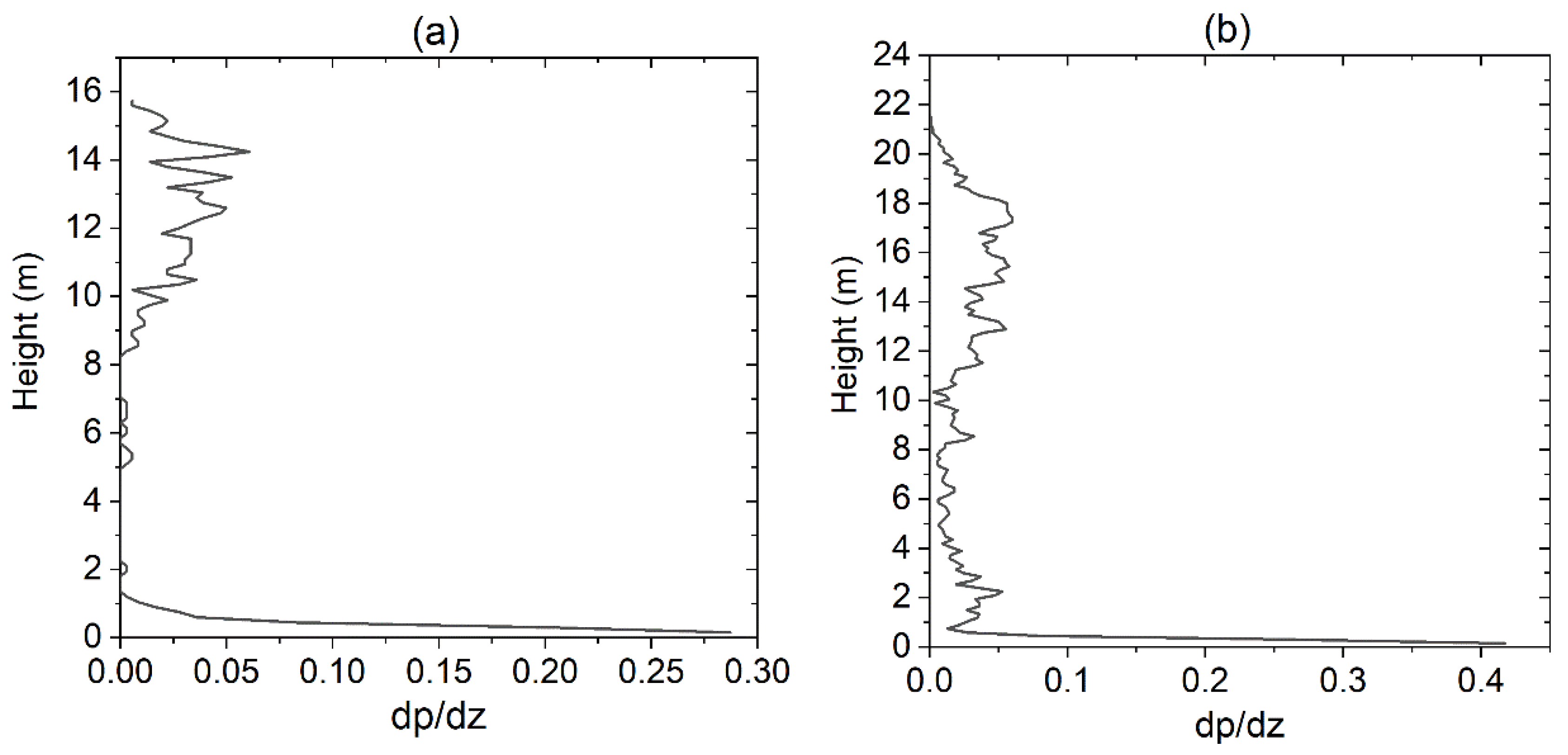
3.1. Determination of the Overstory–Understory Height Boundary at the Plot Level
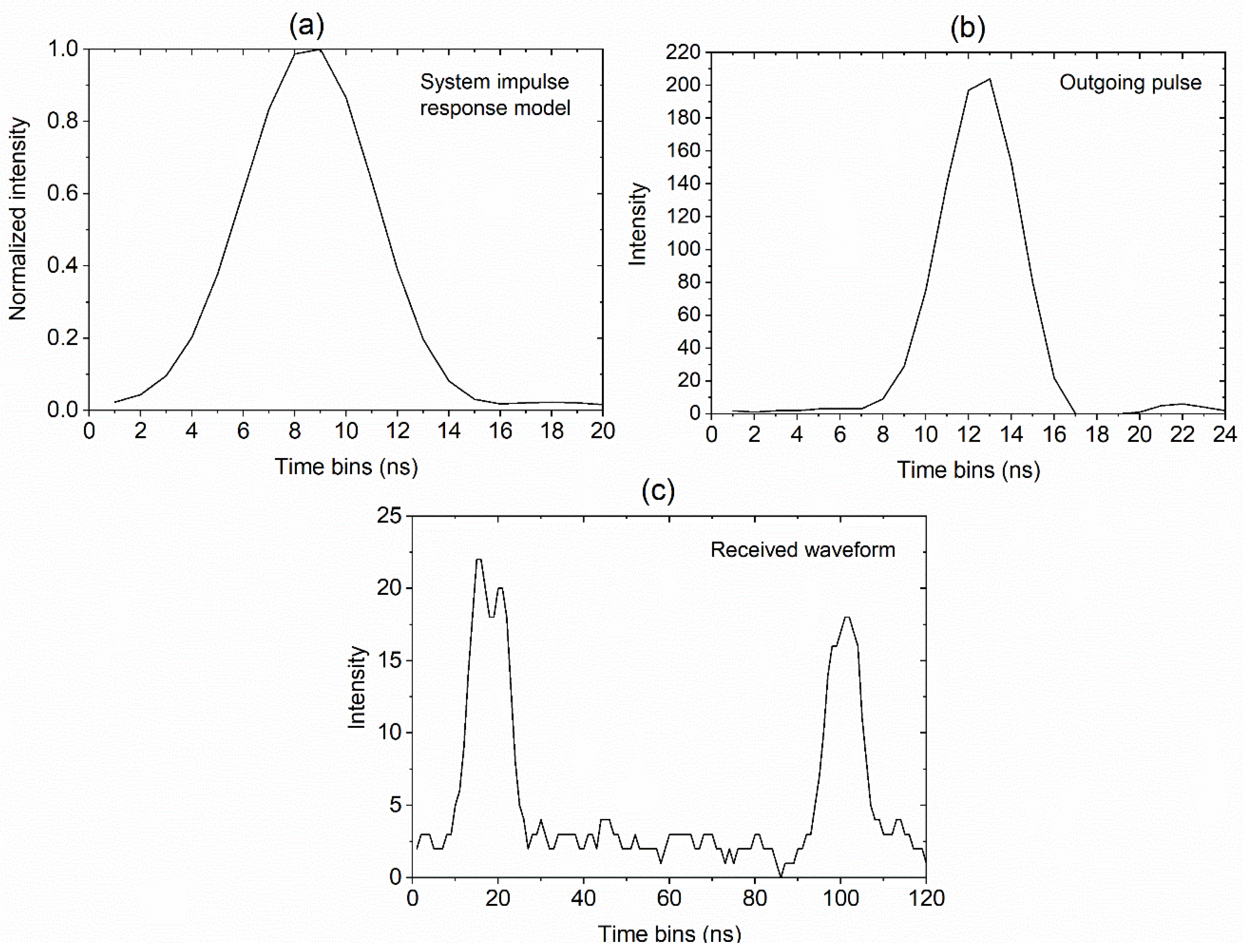
3.2. Preprocessing of Full-Waveform Data
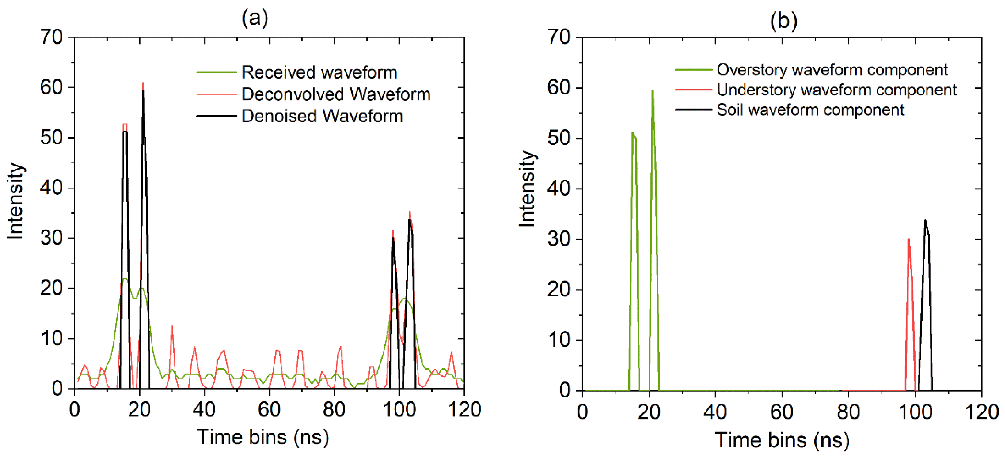
3.2.1. Waveform Deconvolution
3.2.2. Waveform Decomposition
3.3. Retrieval of the Understory LAI
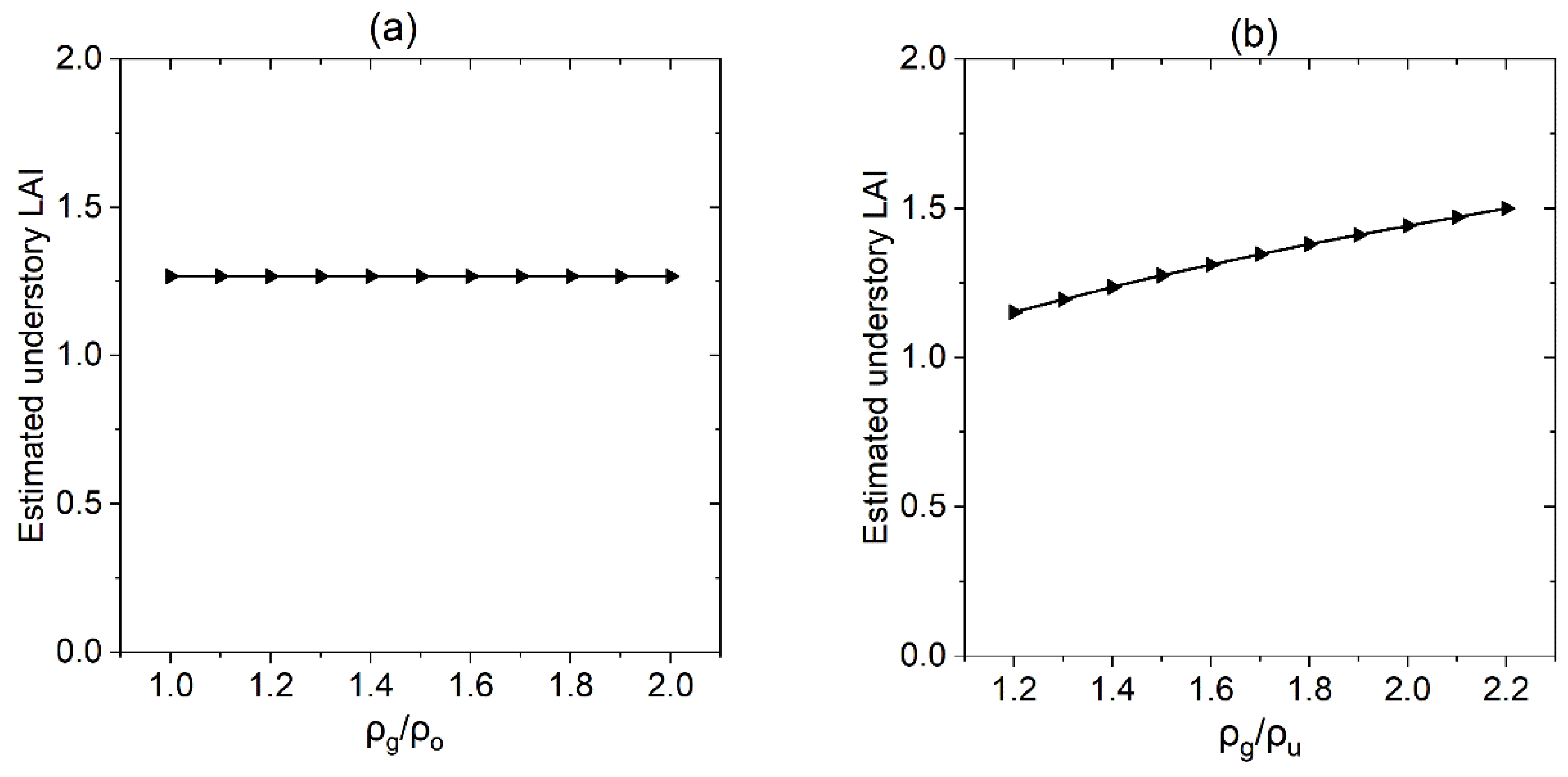
3.4. Sensitivity Analysis of the Spectral Parameters
4. Results
4.1. Overstory–Understory Height Boundary
4.2. Waveforms after Deconvolution and Decomposition
4.3. Sensitivity of the Method to Spectral Parameters
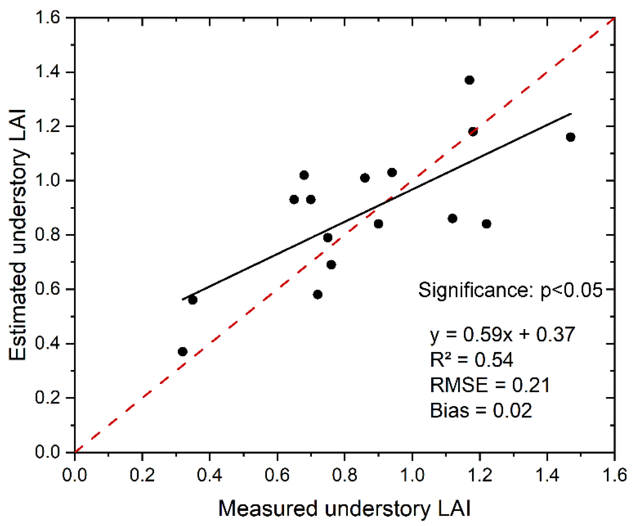
4.4. Retrieved Understory LAI
5. Discussion
6. Conclusions
Author Contributions
Funding
Data Availability Statement
Acknowledgments
Conflicts of Interest
References
- Shugart, H.H.; Saatchi, S.; Hall, F.G. Importance of structure and its measurement in quantifying function of forest ecosystems. J. Geophys. Res. Biogeosciences 2010, 115. [Google Scholar] [CrossRef]
- Sumnall, M.; Fox, T.R.; Wynne, R.H.; Thomas, V.A. Mapping the height and spatial cover of features beneath the forest canopy at small-scales using airborne scanning discrete return Lidar. ISPRS J. Photogramm. Remote Sens. 2017, 133, 186–200. [Google Scholar] [CrossRef]
- Allouis, T.; Durrieu, S.; Couteron, P. A New Method for Incorporating Hillslope Effects to Improve Canopy-Height Estimates From Large-Footprint LIDAR Waveforms. IEEE Geosci. Remote Sens. Lett. 2012, 9, 730–734. [Google Scholar] [CrossRef]
- Armston, J.; Disney, M.; Lewis, P.; Scarth, P.; Phinn, S.; Lucas, R.; Bunting, P.; Goodwin, N. Direct retrieval of canopy gap probability using airborne waveform lidar. Remote Sens. Environ. 2013, 134, 24–38. [Google Scholar] [CrossRef]
- Wang, Y.; Ni, W.J.; Sun, G.Q.; Chi, H.; Zhang, Z.Y.; Guo, Z.F. Slope-adaptive waveform metrics of large footprint lidar for estimation of forest aboveground biomass. Remote Sens. Environ. 2019, 224, 386–400. [Google Scholar] [CrossRef]
- Eskelson, B.N.I.; Madsen, L.; Hagar, J.C.; Temesgen, H. Estimating riparian understory vegetation cover with beta regression and copula models. For. Sci. 2011, 57, 212–221. [Google Scholar]
- Royo, A.A.; Carson, W.P. On the formation of dense understory layers in forests worldwide: Consequences and implications for forest dynamics, biodiversity, and succession. Can. J. For. Res. 2006, 36, 1345–1362. [Google Scholar] [CrossRef]
- Gonzalez-Benecke, C.A.; Samuelson, L.J.; Stokes, T.A.; Cropper, W.P.; Martin, T.A.; Johnsen, K.H. Understory plant biomass dynamics of prescribed burned Pinus palustris stands. For. Ecol. Manag. 2015, 344, 84–94. [Google Scholar] [CrossRef]
- Molina, J.R.; Rodriguez y Silva, F.; Herrera, M.A. Potential crown fire behavior in Pinus pinea stands following different fuel treatments. For. Syst. 2011, 20, 266–267. [Google Scholar] [CrossRef] [Green Version]
- Watson, D.J.; Watson, M.A. Comparative physiological studies on the growth of field crops. Ann. Appl. Biol. 1953, 40, 1–37. [Google Scholar] [CrossRef]
- Chen, J.M.; Black, T.A. Defining leaf area index for non-flat leaves. Plant Cell Environ. 1992, 15, 421–429. [Google Scholar] [CrossRef]
- Chen, J.M.; Cihlar, J. Retrieving leaf area index of boreal conifer forests using landsat TM images. Remote Sens. Environ. 1996, 55, 153–162. [Google Scholar] [CrossRef]
- Ganguly, S.; Nemani, R.R.; Zhang, G.; Hashimoto, H.; Milesi, C.; Michaelis, A.; Wang, W.; Votava, P.; Samanta, A.; Melton, F.; et al. Generating global Leaf Area Index from Landsat: Algorithm formulation and demonstration. Remote Sens. Environ. 2012, 122, 185–202. [Google Scholar] [CrossRef] [Green Version]
- Tang, H.; Brolly, M.; Zhao, F.; Strahler, A.H.; Schaaf, C.L.; Ganguly, S.; Zhang, G.; Dubayah, R. Deriving and validating Leaf Area Index (LAI) at multiple spatial scales through lidar remote sensing: A case study in Sierra National Forest, CA. Remote Sens. Environ. 2014, 143, 131–141. [Google Scholar] [CrossRef]
- Zhu, X.; Skidmore, A.K.; Wang, T.; Liu, J.; Darvishzadeh, R.; Shi, Y.; Premier, J.; Heurich, M. Improving leaf area index (LAI) estimation by correcting for clumping and woody effects using terrestrial laser scanning. Agric. For. Meteorol. 2018, 263, 276–286. [Google Scholar] [CrossRef]
- Luo, T.; Pan, Y.; Ouyang, H.; Shi, P.; Luo, J.; Yu, Z.; Lu, Q. Leaf area index and net primary productivity along subtropical to alpine gradients in the Tibetan Plateau. Glob. Ecol. Biogeogr. 2004, 13, 345–358. [Google Scholar] [CrossRef]
- Sellers, P.J.; Dickinson, R.E.; Randall, D.A.; Betts, A.K.; Hall, F.G.; Berry, J.A.; Collatz, G.J.; Denning, A.S.; Mooney, H.A.; Nobre, C.A. Modeling the Exchanges of Energy, Water, and Carbon Between Continents and the Atmosphere. Science 1997, 275, 502–509. [Google Scholar] [CrossRef] [PubMed] [Green Version]
- Jacquemoud, S.; Verhoef, W.; Baret, F.; Bacour, C.; Zarco-Tejada, P.J.; Asner, G.P.; Francois, C.; Ustin, S.L. PROSPECT plus SAIL models: A review of use for vegetation characterization. Remote Sens. Environ. 2009, 113, S56–S66. [Google Scholar] [CrossRef]
- Zhu, Z.; Piao, S.; Myneni, R.B.; Huang, M.; Zeng, Z.; Canadell, J.G.; Ciais, P.; Sitch, S.; Friedlingstein, P.; Arneth, A.; et al. Greening of the Earth and its drivers. Nat. Clim. Chang. 2016, 6, 791–795. [Google Scholar] [CrossRef]
- Liang, X.; Lettenmaier, D.P.; Wood, E.F.; Burges, S.J. A simple hydrologically based model of land surface water and energy fluxes for general circulation models. J. Geophys. Res. Atmos. 1994, 99, 14415–14428. [Google Scholar] [CrossRef]
- Garrigues, S.; Lacaze, R.; Frederic, B.; Morisette, J.; Weiss, M.; Nickeson, J.; Fernandes, R.; Plummer, S.; Shabanov, N.V.; Myneni, R.B.; et al. Validation and intercomparison of global Leaf Area Index products derived from remote sensing data. J. Geophys. Res. 2008, 113, G02028. [Google Scholar] [CrossRef]
- Skidmore, A.K.; Pettorelli, N.; Coops, N.C.; Geller, G.N.; Hansen, M.; Lucas, R.; Mucher, C.A.; O’Connor, B.; Paganini, M.; Pereira, H.M.; et al. Agree on biodiversity metrics to track from space. Nature 2015, 523, 403–405. [Google Scholar] [CrossRef] [Green Version]
- Kerr, J.; Ostrovsky, M. From space to species: Ecological applications for remote sensing. Trends Ecol. Evol. 2003, 18, 299–305. [Google Scholar] [CrossRef]
- Hall, F.G.; Bergen, K.; Blair, J.B.; Dubayah, R.; Houghton, R.; Hurtt, G.; Kellndorfer, J.; Lefsky, M.; Ranson, J.; Saatchi, S.; et al. Characterizing 3D vegetation structure from space: Mission requirements. Remote Sens. Environ. 2011, 115, 2753–2775. [Google Scholar] [CrossRef] [Green Version]
- Evans, J.S.; Hudak, A.T.; Faux, R.; Smith, A.M.S. Discrete Return Lidar in Natural Resources: Recommendations for Project Planning, Data Processing, and Deliverables. Remote Sens. 2009, 1, 776–794. [Google Scholar] [CrossRef] [Green Version]
- Hill, R.A.; Broughton, R.K. Mapping the understorey of deciduous woodland from leaf-on and leaf-off airborne LiDAR data: A case study in lowland Britain. ISPRS J. Photogramm. Remote Sens. 2009, 64, 223–233. [Google Scholar] [CrossRef]
- Morsdorf, F.; Mårell, A.; Koetz, B.; Cassagne, N.; Pimont, F.; Rigolot, E.; Allgöwer, B. Discrimination of vegetation strata in a multi-layered Mediterranean forest ecosystem using height and intensity information derived from airborne laser scanning. Remote Sens. Environ. 2010, 114, 1403–1415. [Google Scholar] [CrossRef] [Green Version]
- Wing, B.M.; Ritchie, M.W.; Boston, K.; Cohen, W.B.; Gitelman, A.; Olsen, M.J. Prediction of understory vegetation cover with airborne lidar in an interior ponderosa pine forest. Remote Sens. Environ. 2012, 124, 730–741. [Google Scholar] [CrossRef]
- Campbell, M.J.; Dennison, P.E.; Hudak, A.T.; Parham, L.M.; Butler, B.W. Quantifying understory vegetation density using small-footprint airborne lidar. Remote Sens. Environ. 2018, 215, 330–342. [Google Scholar] [CrossRef]
- Gastellu-Etchegorry, J.-P.; Yin, T.; Lauret, N.; Grau, E.; Rubio, J.; Cook, B.D.; Morton, D.C.; Sun, G. Simulation of satellite, airborne and terrestrial LiDAR with DART (I): Waveform simulation with quasi-Monte Carlo ray tracing. Remote Sens. Environ. 2016, 184, 418–435. [Google Scholar] [CrossRef]
- Bechtold, S.; Höfle, B. Helios: A multi-purpose lidar simulation framework for research, planning and training of laser scanning operations with airborne, ground-based mobile and stationary platforms. ISPRS Ann. Photogramm. Remote Sens. Spat. Inf. Sci. 2016, 3, 161–168. [Google Scholar] [CrossRef] [Green Version]
- Sun, G.; Ranson, K.J.; Kimes, D.S.; Blair, J.B.; Kovacs, K. Forest vertical structure from GLAS: An evaluation using LVIS and SRTM data. Remote Sens. Environ. 2008, 112, 107–117. [Google Scholar] [CrossRef]
- Ma, H.; Song, J.; Wang, J. Forest Canopy LAI and Vertical FAVD Profile Inversion from Airborne Full-Waveform LiDAR Data Based on a Radiative Transfer Model. Remote Sens. 2015, 7, 1897–1914. [Google Scholar] [CrossRef] [Green Version]
- Ni-Meister, W.; Jupp, D.L.B.; Dubayah, R. Modeling lidar waveforms in heterogeneous and discrete canopies. IEEE Trans. Geosci. Remote Sens. 2001, 39, 1943–1958. [Google Scholar] [CrossRef] [Green Version]
- Tang, H.; Dubayah, R.; Swatantran, A.; Hofton, M.; Sheldon, S.; Clark, D.B.; Blair, B. Retrieval of vertical LAI profiles over tropical rain forests using waveform lidar at La Selva, Costa Rica. Remote Sens. Environ. 2012, 124, 242–250. [Google Scholar] [CrossRef]
- Tang, H.; Ganguly, S.; Zhang, G.; Hofton, M.A.; Nelson, R.F.; Dubayah, R. Characterizing leaf area index (LAI) and vertical foliage profile (VFP) over the United States. Biogeosciences 2016, 13, 239–252. [Google Scholar] [CrossRef] [Green Version]
- Li, W.; Niu, Z.; Li, J.; Chen, H.Y.; Gao, S.; Wu, M.Q.; Li, D. Generating pseudo large footprint waveforms from small footprint full-waveform airborne LiDAR data for the layered retrieval of LAI in orchards. Opt. Express 2016, 24, 10142–10156. [Google Scholar] [CrossRef]
- Tan, W.; Zhou, L.; Liu, K. Soil aggregate fraction-based C-14 analysis and its application in the study of soil organic carbon turnover under forests of different ages. Chin. Sci. Bull. 2013, 58, 1936–1947. [Google Scholar] [CrossRef] [Green Version]
- Du, Z.; Wang, W.; Zeng, W.; Zeng, H. Nitrogen Deposition Enhances Carbon Sequestration by Plantations in Northern China. PLoS ONE 2014, 9, e87975. [Google Scholar] [CrossRef] [Green Version]
- Pang, Y.; Li, Z.Y.; Ju, H.B.; Lu, H.; Jia, W.; Si, L.; Guo, Y.; Liu, Q.W.; Li, S.M.; Liu, L.X.; et al. LiCHy: The CAF’s LiDAR, CCD and Hyperspectral Integrated Airborne Observation System. Remote Sens. 2016, 8, 398. [Google Scholar] [CrossRef] [Green Version]
- Pablo, C.P.; Piotr, T.; Nicholas, C.; Angel, R.L. Characterizing understory vegetation in Mediterranean forests using full-waveform airborne laser scanning data. Remote Sens. Environ. 2018, 217, 400–413. [Google Scholar] [CrossRef]
- Zhao, X.Q.; Guo, Q.H.; Su, Y.J.; Xue, B.L. Improved progressive TIN densification filtering algorithm for airborne LiDAR data in forested areas. Isprs J. Photogramm. Remote Sens. 2016, 117, 79–91. [Google Scholar] [CrossRef] [Green Version]
- Riaño, D.; Meier, E.; Allgöwer, B.; Chuvieco, E.; Ustin, S.L. Modeling airborne laser scanning data for the spatial generation of critical forest parameters in fire behavior modeling. Remote Sens. Environ. 2003, 86, 177–186. [Google Scholar] [CrossRef]
- Mallet, C.; Bretar, F. Full-waveform topographic lidar: State-of-the-art. ISPRS J. Photogramm. Remote Sens. 2009, 64, 1–16. [Google Scholar] [CrossRef]
- Jalobeanu, A.; Gonçalves, G. The full-waveform LiDAR RIEGL LMS-Q680I: From reverse engineering to sensor modeling. In Proceedings of the American Society for Photogrammetry and Remote Sensing Annual Conference, Sacramento, CA, USA, 19–23 March 2012. [Google Scholar]
- Fish, D.A.; Brinicombe, A.M.; Pike, E.R.; Walker, J.G. Blind deconvolution by means of the Richardson–Lucy algorithm. J. Opt. Soc. Am. Opt. Image Sci. Vis. 1995, 12, 58–65. [Google Scholar] [CrossRef] [Green Version]
- Wu, J.; Van Aardt, J.A.N.; Asner, G.P. A comparison of signal deconvolution algorithms based on small-footprint LiDAR waveform simulatioin. IEEE Trans. Geosci. Remote Sens 2011, 40, 2402–2414. [Google Scholar] [CrossRef]
- Savitzky, A.; Golay, M.J.E. Smoothing and Differentiation of Data by Simplified Least Squares Procedures. Anal. Chem. 1964, 36, 1627–1639. [Google Scholar] [CrossRef]
- Wagner, W.; Ullrich, A.; Ducic, V.; Melzer, T.; Studnicka, N. Gaussian decomposition and calibration of a novel small-footprint full-waveform digitising airborne laser scanner. ISPRS J. Photogramm. Remote Sens. 2006, 60, 100–112. [Google Scholar] [CrossRef]
- Boggs, P.; Tolle, J. Sequential Quadratic Programming. Acta Numer. 1995, 4, 1–51. [Google Scholar] [CrossRef] [Green Version]
- Chen, J.M.; Cihlar, J. Plant canopy gap-size analysis theory for improving optical measurements of leaf-area index. Appl. Opt. 1995, 34, 6211–6222. [Google Scholar] [CrossRef] [PubMed] [Green Version]
- Chen, J.M.; Rich, P.M.; Gower, S.T.; Norman, J.M.; Plummer, S. Leaf area index of boreal forests: Theory, techniques, and measurements. J. Geophys. Res. Atmos. 1997, 102, 29429–29443. [Google Scholar] [CrossRef]
- Tang, H.; Dubayah, R.; Brolly, M.; Ganguly, S.; Zhang, G. Large-scale retrieval of leaf area index and vertical foliage profile from the spaceborne waveform lidar (GLAS/ICESat). Remote Sens. Environ. 2014, 154, 8–18. [Google Scholar] [CrossRef]
- Tian., J.; Philpot, W.D. Spectral reflectance of drying soil. In Proceedings of the IEEE Geoscience and Remote Sensing Symposium, Quebec, QC, Canada, 13–18 July 2014; pp. 3259–3262. [Google Scholar]
- Wu, Q.; Song, C.; Song, J.; Wang, J.; Bo, Y. Impacts of Leaf Age on Canopy Spectral Signature Variation in Evergreen Chinese Fir Forests. Remote Sens. 2018, 10, 262. [Google Scholar] [CrossRef] [Green Version]
- Chavana-Bryant, C.; Malhi, Y.; Anastasiou, A.; Enquist, B.J.; Cosio, E.G.; Keenan, T.F.; Gerard, F.F. Leaf age effects on the spectral predictability of leaf traits in Amazonian canopy trees. Sci. Total Environ. 2019, 666, 1301–1315. [Google Scholar] [CrossRef] [PubMed] [Green Version]
- Gara, T.W.; Darvishzadeh, R.; Skidmore, A.K.; Wang, T. Impact of Vertical Canopy Position on Leaf Spectral Properties and Traits across Multiple Species. Remote Sens. 2018, 10, 346. [Google Scholar] [CrossRef] [Green Version]


| Understory LAI | |
|---|---|
| Min | 0.32 |
| Max | 1.47 |
| Mean | 0.86 |
| SD | 0.31 |
| Range | 1.15 |
| Plot ID | Height Boundary | Plot ID | Height Boundary |
|---|---|---|---|
| 1 | 1.35 | 9 | 1.50 |
| 2 | 3.90 | 10 | 2.40 |
| 3 | 3.30 | 11 | 2.40 |
| 4 | 2.10 | 12 | 3.60 |
| 5 | 3.90 | 13 | 2.00 |
| 6 | 3.90 | 14 | 2.10 |
| 7 | 2.85 | 15 | 1.05 |
| 8 | 1.50 | 16 | 2.00 |
Publisher’s Note: MDPI stays neutral with regard to jurisdictional claims in published maps and institutional affiliations. |
© 2021 by the authors. Licensee MDPI, Basel, Switzerland. This article is an open access article distributed under the terms and conditions of the Creative Commons Attribution (CC BY) license (https://creativecommons.org/licenses/by/4.0/).
Share and Cite
Song, J.; Zhu, X.; Qi, J.; Pang, Y.; Yang, L.; Yu, L. A Method for Quantifying Understory Leaf Area Index in a Temperate Forest through Combining Small Footprint Full-Waveform and Point Cloud LiDAR Data. Remote Sens. 2021, 13, 3036. https://doi.org/10.3390/rs13153036
Song J, Zhu X, Qi J, Pang Y, Yang L, Yu L. A Method for Quantifying Understory Leaf Area Index in a Temperate Forest through Combining Small Footprint Full-Waveform and Point Cloud LiDAR Data. Remote Sensing. 2021; 13(15):3036. https://doi.org/10.3390/rs13153036
Chicago/Turabian StyleSong, Jinling, Xiao Zhu, Jianbo Qi, Yong Pang, Lei Yang, and Lihong Yu. 2021. "A Method for Quantifying Understory Leaf Area Index in a Temperate Forest through Combining Small Footprint Full-Waveform and Point Cloud LiDAR Data" Remote Sensing 13, no. 15: 3036. https://doi.org/10.3390/rs13153036