Article

Using Multi-Temporal Satellite Data to Analyse Phenological Responses of Rubber (Hevea brasiliensis) to Climatic Variations in South Sumatra, Indonesia

by
Fathin Ayuni Azizan
1,2,*,
Ike Sari Astuti
3,
Mohammad Irvan Aditya
3,
Tri Rapani Febbiyanti
4,
Alwyn Williams
1,
Anthony Young
1 and
Ammar Abdul Aziz
1
1
School of Agriculture and Food Sciences, The University of Queensland, Gatton, QLD 4343, Australia
2
Faculty of Chemical Engineering Technology, Universiti Malaysia Perlis, Arau 02600, Perlis, Malaysia
3
Department of Geography, Universitas Negeri Malang, Malang 65145, Jawa Timur, Indonesia
4
Indonesian Rubber Research Institute, Medan 30953, South Sumatra, Indonesia
*
Author to whom correspondence should be addressed.
Remote Sens. 2021, 13(15), 2932; https://doi.org/10.3390/rs13152932
Submission received: 18 June 2021 / Revised: 21 July 2021 / Accepted: 22 July 2021 / Published: 26 July 2021
(This article belongs to the Section Environmental Remote Sensing)

Abstract

:
Land surface phenology derived from satellite data provides insights into vegetation responses to climate change. This method has overcome laborious and time-consuming manual ground observation methods. In this study, we assessed the influence of climate on phenological metrics of rubber (Hevea brasiliensis) in South Sumatra, Indonesia, between 2010 and 2019. We modelled rubber growth through the normalised difference vegetation index (NDVI), using eight-day surface reflectance images at 250 m spatial resolution, sourced from NASA’s Moderate Resolution Imaging Spectroradiometer (MODIS) Terra and Aqua satellites. The asymmetric Gaussian (AG) smoothing function was applied on the model in TIMESAT to extract three phenological metrics for each growing season: start of season (SOS), end of season (EOS), and length of season (LOS). We then analysed the effect of rainfall and temperature, which revealed that fluctuations in SOS and EOS are highly related to disturbances such as extreme rainfall and elevated temperature. Additionally, we observed inter-annual variations of SOS and EOS associated with rubber tree age and clonal variability within plantations. The 10-year monthly climate data showed a significant downward and upward trend for rainfall and temperature data, respectively. Temperature was identified as a significant factor modulating rubber phenology, where an increase in temperature of 1 °C advanced SOS by ~25 days and EOS by ~14 days. These results demonstrate the capability of remote sensing observations to monitor the effects of climate change on rubber phenology. This information can be used to improve rubber management by helping to identify critical timing for implementation of agronomic interventions.

Graphical Abstract

1. Introduction

Phenology refers to the study of the recurring stages of plant and animal life [1]. Vegetation phenology studies specific plant life cycle events such as bud burst, canopy growth, flowering, and senescence, and their relation to environmental factors. Phenology is a robust ecological indicator of climate change [2,3] and environmental variation impacts, across individual species to entire landscapes [4]. Most phenological events are receptive to temperature, rainfall, and human activities that affect vegetation growth and functions. For example, previous studies have linked shifts in rainfall and temperature to delayed leaf senescence and abscission in rubber trees [5], earlier start of the growing season across species in Ethiopia [6], advances in leaf unfolding of several woody species [7], and reduced litter components in three Acacia species [8]. Thus, phenology facilitates an improved understanding of the interactions among biotic and abiotic factors that impact life on Earth.
Two commonly employed techniques to study vegetation phenology are ground observation [5,9] and remote sensing (e.g., [10,11]). Ground observation data are used for conducting species-specific phenological analyses at limited scales [9,12]. This technique is time and resource expensive. Alternately, general inter-annual vegetation changes can be interpreted via spatial and spectral resolutions of remote sensing imagery, although this does not include specific phenological events [13]. This is called land surface phenology. It captures larger landscapes [14] over longer timeframes [15] in order to define the land surface phenological metrics of growing seasons. The most commonly used metrics are start, end, and length of growing season (SOS, EOS, and LOS, respectively) [16,17]. The SOS and EOS are important phenological metrics as they are the termini wherein vegetation phenological events occur.
Various types of satellite data have been used to monitor land surface phenology. These include Deep Space Climate Observatory (DSCOVR) satellites data [18], geostationary satellites data (e.g., GEOS-16 and -17 [19]), polar orbit satellites data (e.g., MODIS [11,20,21] and Landsat [22,23,24]) and solar-induced fluorescence (SIF) data [25,26,27]. Geostationary satellites provide the highest temporal resolution of 30 to 2.5 min, followed by MODIS at 1-day, and SIF at 16-days. Although higher temporal resolutions are crucial in phenology monitoring, the selection of satellite data is subject to a trade-off between spatial and temporal resolution and is limited by its coverage.
Most land surface phenology models are derived from vegetation indices extracted from satellite data. The most widely used vegetation indices for this purpose are Normalised Difference Vegetation Index (NDVI) [28,29] and Enhanced Vegetation Index (EVI) [30,31]. For remote sensing, vegetation phenology is the integrative environmental indicator of climate change, which reveals the impacts of climate change on vegetation phenology over space and time. Broich et al. [10] studied the land surface phenology response to climate variability across Australia. They modelled the phenological cycle curves from EVI-measured greening and browning, and extracted the key phenological metrics from it. Their result indicates that phenological metrics of cycle peak and integrated greenness were significantly correlated to the standardised difference in air pressure as opposed to rainfall. On the other hand, Moses et al. [20] found that rainfall influences land surface phenology metrics during the green-up period but not in the senescence period in the semi-arid savanna of South Africa. In their study, the SOS and EOS phenological metrics were derived from analysis of a time series of leaf area index. Similarly, using NDVI data, Wang et al. [32] extracted the same phenological metrics to study climate and phenology interactions in catchment areas in the Northern Hemisphere, showing that an increase in temperature strongly influenced the advance of SOS and delay of EOS in the study area. Busetto et al. [33] compared field data with NDVI extracted SOS and EOS, concluding that NDVI enabled more accurate estimates for the two metrics. This study also reported that an increase in mean spring temperature leads to the advancement of budburst. This technique has also been applied to conifer forest [34] and alpine forest [35] to study the land surface phenology of the crop. However, the study of land surface phenology of plantation crops such as rubber (Hevea brasiliensis) is still relatively unexplored.
Rubber is a plantation crop that produces latex. The key phenological stages that occur in rubber involve annual defoliation and refoliation processes during what is called the wintering period. Wintering occurs in the dry season, which in Sumatra is between July and September. Leaf fall in the refoliation period naturally causes distinct changes in the tree canopy. This biophysical property is an excellent indicator for detecting, measuring, and tracking growth using remote sensing imagery. Previous studies have exploited this unique characteristic to differentiate rubber from other vegetation, such as forest and oil palm, for mapping purposes [36,37,38]. Several vegetation indices such as NDVI, Land Surface Water Index (LSWI), Normalized Burn Ratio (NBR), Atmospherically Resistant Vegetation Index (ARVI), and Normalised Difference Moisture Index (NDMI) have been effectively deployed for detection of wintering in rubber [39,40]. Rubber phenology is highly sensitive to climate change, particularly to rainfall and temperature [9,41,42]. These responses have a direct impact on yield [43]. The SOS and EOS are affected by temperature and rainfall, respectively, as changes in these climatic factors may delay or advance the season [9]. Our knowledge on how climatic factors influence land surface phenology metrics such as SOS and EOS is currently limited. To our knowledge, no previous study has investigated and analysed phenological trends using multi-temporal remote sensing data for rubber plantations. This is particularly important as rubber plantations have a relatively long economic lifespan of up to 35 years.
In this study, we aimed to investigate the influence of climate on rubber phenological changes over the past ten years using remote sensing datasets. The specific objectives of the paper are three-fold: (1) to demonstrate the applicability of remote sensing data to extract the rubber phenology of SOS and EOS; (2) to examine the trend and changes of two major climatic data; and (3) to assess SOS/EOS response to rainfall and temperature. This information is essential for differentiating natural leaf drop during wintering with abnormal leaf drop. Consequently, this could assist in developing an early warning system for disease and triggering interventions.

2. Materials and Methods
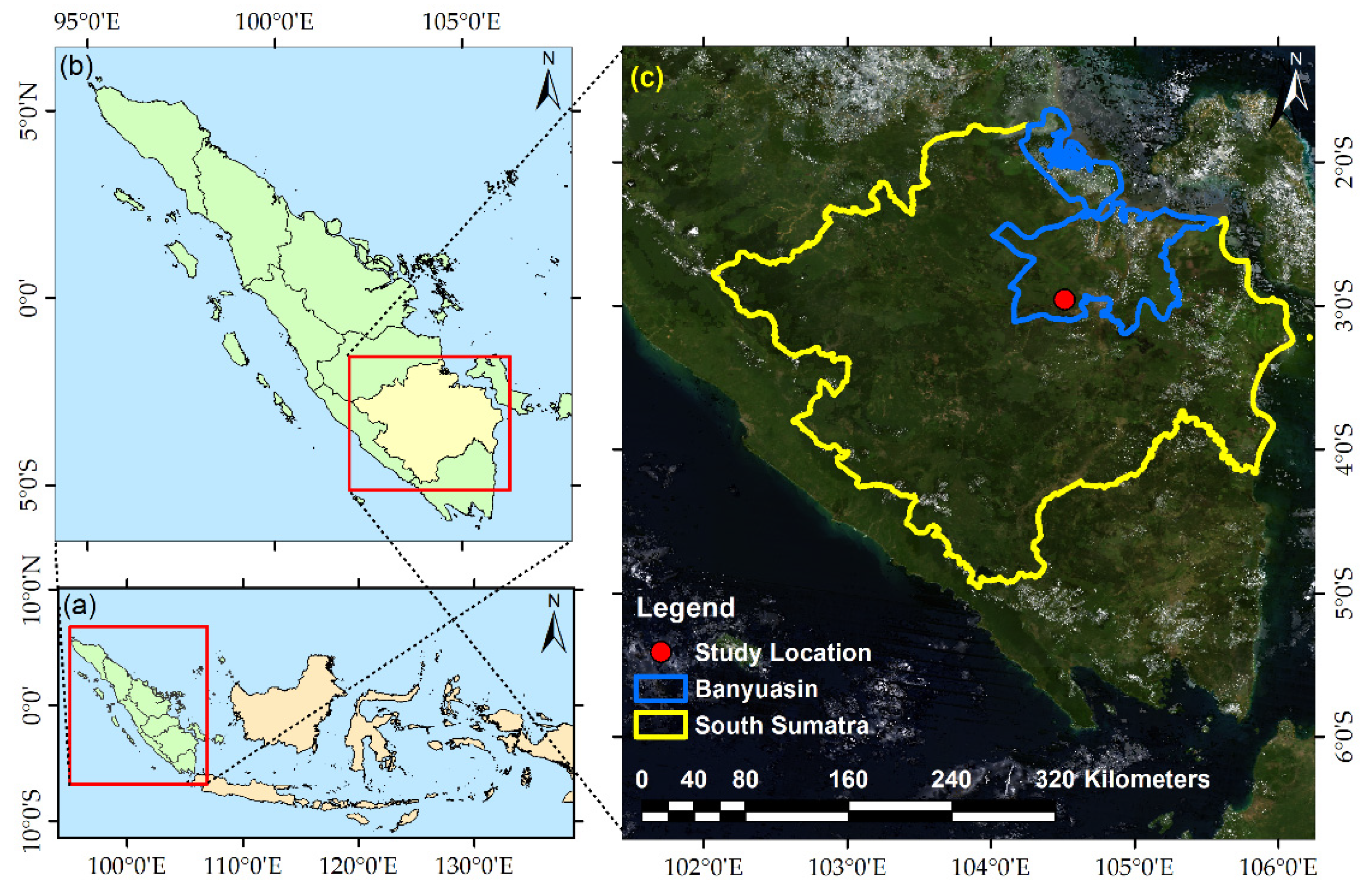
2.1. Study Area

Indonesia has the largest area planted to rubber in the world. Among all Indonesian provinces, South Sumatra (3.3194°S and 103.9144°E) possesses the largest area committed to rubber production. The province contributed 28.1% of total Indonesian dry rubber production in the year 2018 [44]. Within South Sumatra, agriculture is the pillar of the economy, with natural rubber being particularly important. Therefore, South Sumatra, specifically in the Banyuasin regency, was chosen as a study area, covering a total area of 1493 hectares (Figure 1).
The study area is characterised by a tropical monsoon climate that delivers annual dry and rainy seasons. The dry season typically spans from May to September, while the rainy season falls between October and April. The average annual precipitation is 2623 mm, with air temperature ranging from 24.7 °C to 32.9 °C and relatively high air humidity above 82%. The average altitude of the area is approximately 8 m.
Rubber plantations were the sole land cover type analysed in this study, and there was no change in land cover type throughout the study period of 2010 to 2019. This minimised uncertainties in the remote sensing data pixels as there was no influence of other crops/land cover when extracting rubber phenology.

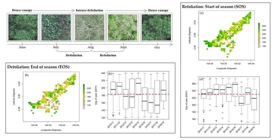
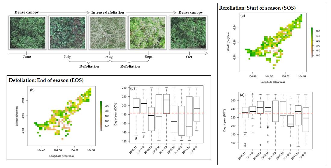
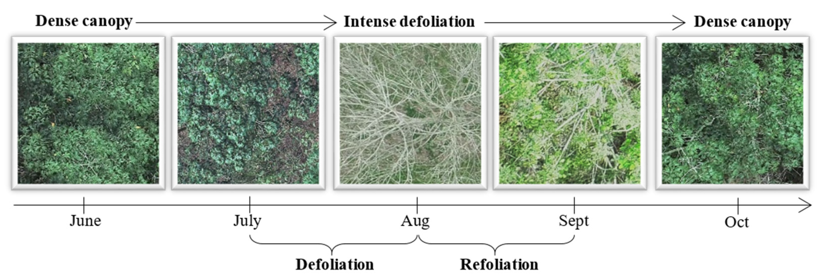
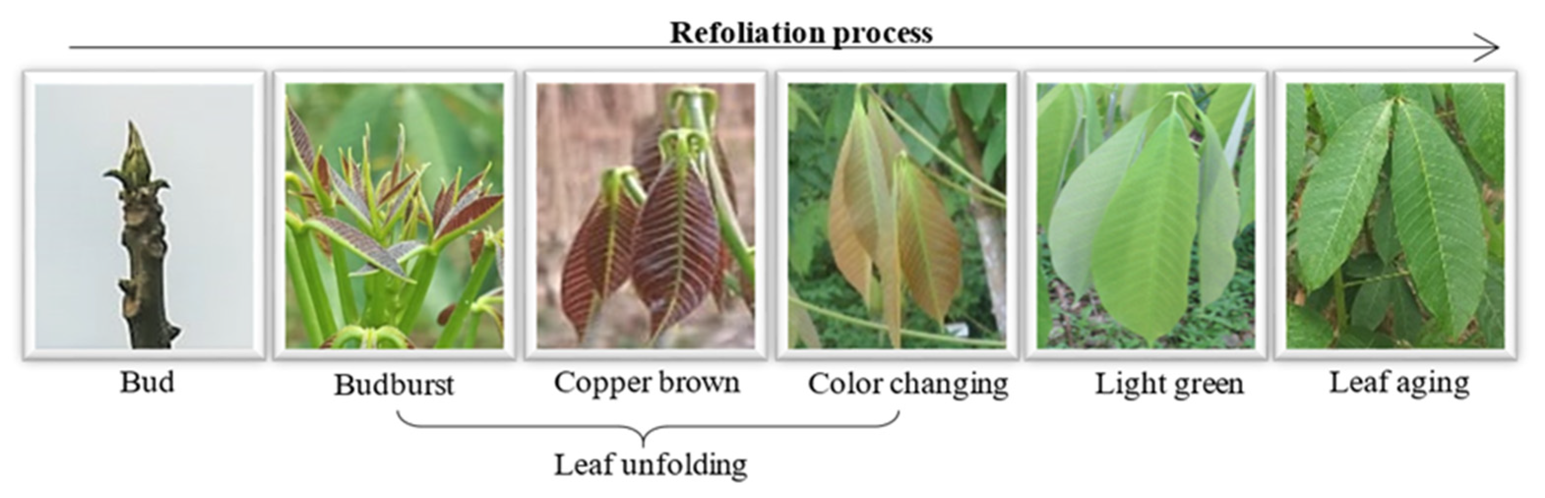
2.2. Rubber Phenological Events and Remote Sensing

Rubber trees are considered mature and ready for latex harvesting at 5–7 years. At full maturity, rubber trees commence annual wintering behaviour, where leaves are shed during the drier months before being replaced with fresh foliage.
Prior to defoliation, the normally dark green, mature leaves turn brown-yellow before they fall. This takes approximately three to four weeks [45] and indicates the end of the growing season. In the refoliation period, the new leaves emerge and expand. This is considered the start of the growing season. The changes in canopy density are dramatic and are illustrated in Figure 2. The images were taken one month apart using an unmanned aerial vehicle. At the canopy level, the leaf colour indicates the age or maturity of leaves, and intense defoliation marks the junction between the defoliation and refoliation process. During refoliation, emerging leaves change from a reddish colour to green (Figure 3). Similar phenological stages during rubber leaf development have been previously reported [9]. The whole process of defoliation and refoliation takes approximately six to eight weeks and occurs in the dry season, typically May to September for South Sumatra, Indonesia. Plant metabolism is substantially affected during this period, with latex production decreasing up to 60% from the peak. The phenological stages in the wintering period are strongly influenced by climatic factors [45]. Apart from this period, the tree maintains a full canopy of leaves throughout the year.

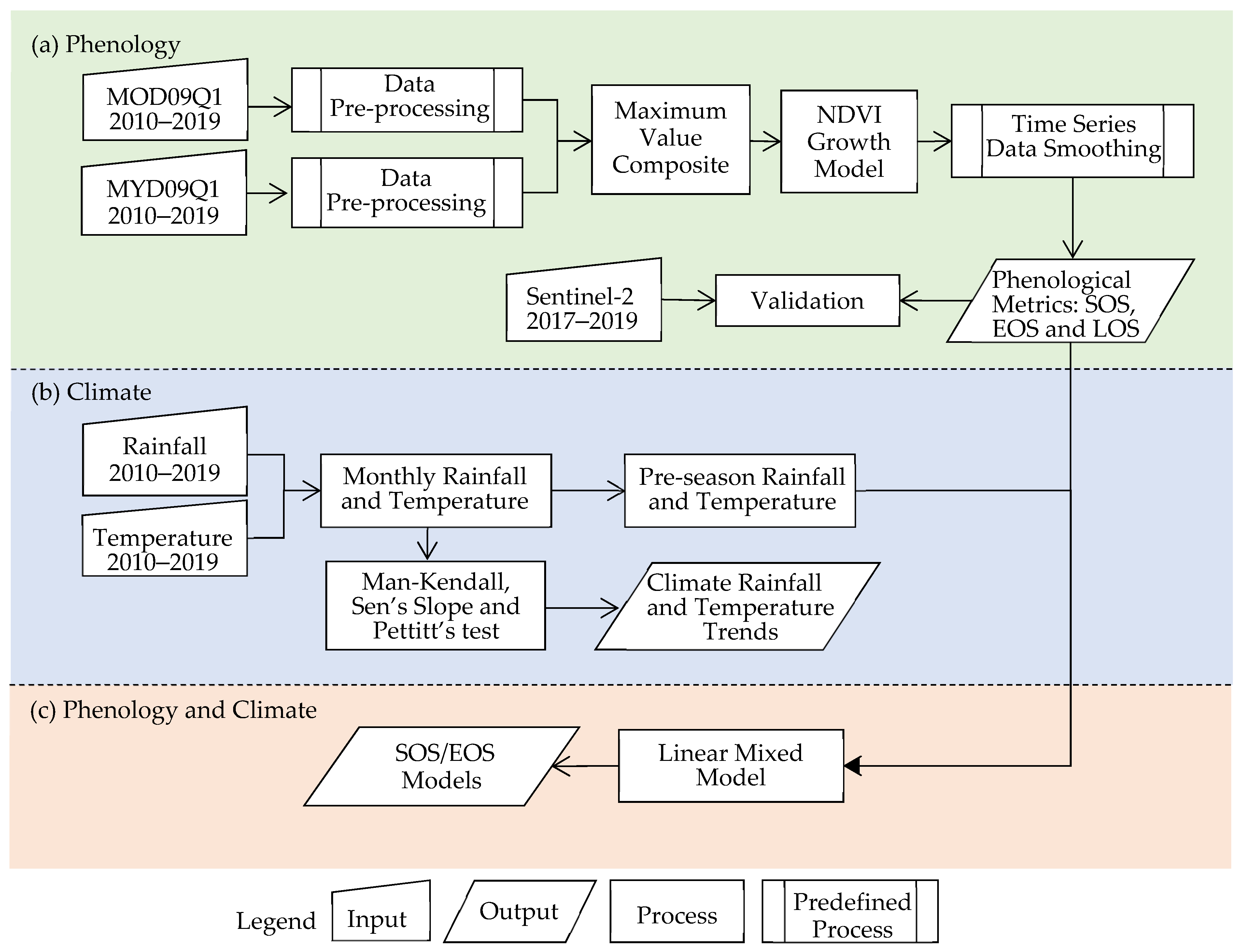
2.3. Method Overview

Figure 4 illustrates an overview of the methods used to investigate the influence of climate on rubber phenology. The flowchart is divided into three major sections: (1) phenology; (2) climate; and (3) phenology and climate. Each section describes the flowchart of obtaining the phenological metrics, climate rainfall, and temperature trends, and SOS/EOS models, respectively. The flowchart symbols are defined at the bottom of the chart. Based on the symbols, there are five input datasets used in this study: MODIS MOD09Q1, MODIS MYD09Q1, Sentinel-2, rainfall, and temperature data. The details of each process involved are further explained in the following subsection of this paper.

2.4. Remote Sensing Data

The remote sensing data used in this study are from MODIS and Sentinel-2. The MODIS datasets were the primary dataset, while the Sentinel-2 data were used for validation purposes. The subsection below describes the reasons for the selection of these datasets and the pre-processing and processing steps conducted on the image datasets.

2.4.1. Selection of Base Data and Generation of NDVI

In this study, 10 years (2010–2019) of satellite data from the Moderate Resolution Imaging Spectrometer (MODIS) instrument aboard the Terra and Aqua satellites were used. The MODIS data products used for this study are MOD09Q1 and MYD09Q1. These data were selected as they fulfil two study criteria: (1) they cover a 10-year study period; and (2) they offer high frequency temporal data. These data also deliver a better trade-off between spatial and temporal resolution at 250 m and 1-day revisit intervals compared to other remote sensing data and their availability. In this study, low spatial resolution pixels were appropriate given the size of the rubber plantation and absence of confounding land cover uses. High-frequency temporal data at 1-day intervals were required to capture the relatively small window of the rubber wintering period, as well as to mitigate against the impacts of frequent cloud cover associated with the study region.
Although MODIS offers several other products, they were not suitable for this study due to: (1) low data availability, as at least three clear observations within the composite period are needed to process the BRDF inverted observation [46]; (2) overestimation of clouds, particularly in Southeast Asia [47]; (3) the MOD13 products are at a coarse resolution; and (4) the product shortens the growing season compared to other commonly used vegetation indices (VIs) for deriving phenological metrics [48].
Hence, we utilised the surface reflectance composite products of MOD09Q1 and MYD09Q1. The value in each pixel of these products was selected from all data acquisition during an 8-day period by considering low view angle, high observation coverage, the absence of clouds or cloud shadow, and aerosol loading. The data were corrected for atmospheric conditions such as gasses, aerosols, and Rayleigh scattering. The data offer two bands: red (0.620–0.670 µm) and near infrared (0.841–0.876 µm). To further mitigate against persistent cloud cover, MOD09Q1 and MYD09Q1 data were combined to increase data availability for interpolation and smoothing processes while addressing issues associated with cloud cover. Both data sets showed high compatibility [49,50], and it has been previously shown that they can be used in combination [51].
In total, 920 images of MODIS tile h28v09 were downloaded from the USGS website (https://earthexplorer.usgs.gov/ (accessed on 1 February 2020)). The NDVI time-series data were used to represent the rubber growth cycle. Previously, NDVI values have shown utility in reflecting the greenness and consequently health status of vegetation, and have been recently employed in several phenological studies [34,52]. It is the most commonly applied VI in optical remote sensing observations to estimate key phenological events [6,11,30,53]. The NDVI is sufficiently stable to facilitate comparisons of inter-annual variations of vegetation while reducing noise [48]. In this study, the NDVI [54] values were calculated using Equation (1) where Band 1 is the red band and Band 2 is the near infrared band:
NDVI = (Band 2 − Band 1)/(Band 2 + Band 1).

2.4.2. Data Pre-Processing

The NDVI datasets underwent several pre-processing steps to prepare data for interpolation and data smoothing before seasonal parameters were identified and extracted. The pre-processing steps involved were pre-projection of the coordinate system, removal of bad data/outlier, cloud masking, rubber area masking, applying scale factor, combining both datasets using the maximum-value composite (MVC) [55] procedure on pixel-by-pixel basis and converting the data to readable file format. The outliers were removed based on pixel reliability information from MODIS. The cloud state information for each image was downloaded and used for cloud masking. The combination of datasets was conducted using the ArcGIS image analysis tool. All other steps were undertaken in RStudio software.

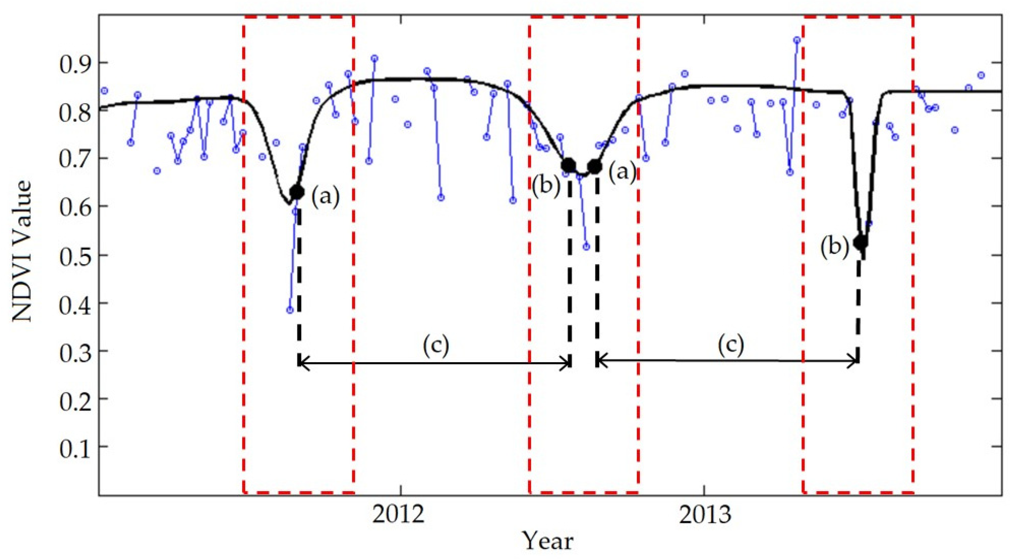
2.4.3. Time Series Data Smoothing

We applied a smoothing method to the NDVI time-series using TIMESAT software (v3.1.1) to model the rubber phenological metrics. This software is a free software package, developed by Lars Eklundh and Per Jonsson, and offers seasonality computation of satellite time-series data while relating the relationship to phenological properties of vegetation [56]. Hird and McDermid [57], after evaluating several freely available software packages offering similar functionality to TIMESAT, concluded that the models used in TIMESAT are highly competitive and able to preserve signal integrity.
Several recent studies employed this approach on various MODIS data products to study the phenology of croplands from several regions including the Yangtze River Delta [58], Sri Lanka [59], California [60], and North America [61]. They have applied one or more of the three smoothing methods in TIMESAT: asymmetric Gaussian (AG), Savitzky-Golay (SG), and Double Logistic (DL) [56]. Smoothing needs to be applied because raw time series data may contain residual noise or spikes caused by disturbance from atmospheric conditions [21], while retaining the seasonal curve [34].
In this study, the AG smoothing method was applied to the NDVI time series. This method was chosen because it is robust and tends to eliminate noise in peak and valley time series. Additionally, it helps reconstruct seasonal patterns when the data are noisy [62]. Tan et al. [63] found AG function to be less sensitive to noise and missing data. The formula for the AG smoothing method used is presented in Equation (2):
g(t;x1.x2.….x5) = {exp exp [−((t − x1)/x2) x3 ] if t > x1 exp exp [−((x1 − t)/x4) x5]
if t < x1,
where t is time, x1 determines the maximum or minimum position of the independent time variable, x2, x3 determine the width and flatness of the right function half, and x4 and x5 determine the width and flatness of left half.
The seasonal parameter and adaptation strength were set to 1 and 2, respectively. The spike method of median filter was used to reduce noise in satellite time series data. The seasonal parameters were set to 1 because the rubber sheds its leaves once a year.

2.4.4. Derivation of Phenological Metrics

Seasonal phenological metrics from 8-day NDVI MODIS time series were derived on a pixel basis for the study area whenever TIMESAT recognised full seasons. Figure 5 shows an example of two seasons detected from a three-year MODIS NDVI dataset from 2011 to 2013. These metrics define the phenological profiles and enable interpretation of results [23]. They also reveal the relationship between NDVI and the phenology of the rubber, where NDVI values in the study reflect the canopy cover and hence the tree health of the rubber plantation. In this process, model input variables of 460 NDVI values of each pixel were reduced to nine phenological metrics with a maximum of nine seasons identified.
Using these parameters, three important seasonal parameters were identified. These are the start of season (SOS), end of season (EOS), and length of season (LOS). The SOS indicates the beginning of the season, and normally refers to the transition date in which there is a significant increase in NDVI values. EOS indicates the end of the season where there is a significant decrease in NDVI values [29]. LOS is defined by the duration from start (SOS) to end of season (EOS) [64]. In TIMESAT, SOS and EOS dates are determined using thresholds of seasonal amplitude [61]. In this study, SOS and EOS refers to the day of year (DOY) when 20% of the seasonal amplitude was reached from the left (start of season) or right (end of season) of a particular seasonal profile.
We then used the values of SOS, EOS, and LOS to develop boxplots for the purpose of portraying the dynamics of these values during a 10-year time window. The fluctuations that occurred in these seasonal parameters were analysed and related to events that were documented during that particular year so as to understand and predict the causes.

2.4.5. Validation

Previous studies have used either gross primary production (GPP) flux data from FLUXNET [29,65] or Phenocam [66] or both [67] to validate their satellite-derived phenological metrics. Unfortunately, these datasets were not available in the study area as there is no flux tower station or Phenocam in Indonesia. The nearest flux tower station is in Malaysia, some 660 km away from our study area. Therefore, the validation of satellite-based phenological metrics in this study cannot be made with phenological metrics derived from ground data. While most remote sensing studies have used higher spatial resolution images for accuracy or validation purposes, fewer studies used them to validate phenological metrics. Two recent studies have compared phenological parameters derived from higher spatial resolution satellite data [68,69].
We validated the NDVI model using high spatial resolution data. Initially, data from three satellites (Sentinel, Landsat, and Planet), which offer better spatial resolution than MODIS, were selected for this purpose. After the pre-processing steps, only the Sentinel-2 had sufficient data for further processing in TIMESAT. Planet data shows the lowest percentage in terms of data availability and area coverage in the study area, while Landsat only offers a few images during the wintering period and is prone to the impacts of cloud cover.
Therefore, the Sentinel-2 data (Sentinel-2A and Sentinel-2B) were chosen to validate the MODIS NDVI phenology model in this study. These data provide 10 m spatial resolution with 5-day temporal resolutions. Three years of data between 2017 and 2019 were used for validation because Sentinel-2B was launched in early 2017. Data were downloaded from USGS Earth Explorer platform. It is a level 1C processing product and is geometrically refined. The pixels in this product provide Top-Of-Atmosphere (TOA) reflectance. We first applied atmospheric corrections before removing the clouds and resampled it to 250 m. During the analysis in TIMESAT, a similar process of time-series data smoothing and setting was applied. Although three full-year data were used, only two complete growing seasons were detected and used for comparison. This is because the rubber season in the study area started and ended around middle of the year, and TIMESAT is programmed to only extract the phenological metrics of a complete growing season.

2.5. Climate Data

Rainfall and temperature data from 2010 to 2019 were used in this study. Hourly temperature and rainfall were retrieved from the weather station located within the study area at 2°55′38.2″S and 104°32′20.0″E. We processed and calculated the average daily temperature and cumulative rainfall for all years. The average temperatures were computed for daily, monthly, and yearly periods from the maximum and minimum temperatures recorded. The same process was conducted on rainfall data, only that rainfall data were represented by an accumulation of the rainfall recorded. The monthly average temperature and rainfall accumulation was used for the climatic data test.
For the mixed model analysis, we used an average daily temperature and rainfall accumulation data based on 90-day preseason period, prior to SOS and EOS start date. This period represents the critical climatic window for phenology and was selected in reference to studies conducted by Ren et al. [11] and Cho et al. [20].

2.6. Data Analysis and Statistical Methods

We first computed the spatial distribution of mean SOS/EOS/LOS for the period 2010 to 2019. The variations in SOS/EOS dates at the pixel level were analysed to identify the underlying causes. Then, we presented the inter-annual SOS, EOS, and LOS dates extracted from TIMESAT software for nine growing seasons using the boxplot. Each boxplot displays the first quartile, median, and third quartile of the yearly phenological metrics. In addition, the overall mean of 10-year SOS, EOS, and LOS was also calculated and shown in the representative boxplots. The advance and delay in SOS/EOS dates were assessed and correlated to the events occurring during those particular times using climate data. Any extreme weather and climate events during the 10-year period were also noted. We computed the mean, median, standard deviations, and dispersion index for each phenological metric to evaluate the degree of fluctuation or dispersion in the dataset. The accuracy of the MODIS-based SOS/EOS/LOS were evaluated and validated against the Sentinel-based SOS/EOS/LOS for two growing seasons (2017/18 and 2018/19). Comparisons were made using one-way analysis of variance (ANOVA).
The Mann-Kendall test was applied to evaluate the significance of climatic trend data. It is the most widely used test in the field of meteorology because of its suitability for abnormal distribution data [70]. This test also offers better results for time-series data compared with straight linear functions. Ten years of monthly climatic data for total rainfall and average monthly temperatures were used for this purpose. This test reveals the presence or absence of upward or downward monotonic trends in the total rainfall/average temperature time series data. The results were evaluated based on the p-value and Tau values. The magnitude of the increase or decrease in the climate trend was evaluated using Sen’s slope test. Pettitt’s test for single change point detection was conducted when there was a monotonic trend in the data.
Finally, using selected pre-SOS/EOS climate data and the SOS/EOS of each growing season, we fitted linear mixed models with the SOS/EOS as the outcome, rainfall and/or temperature as predictor variables, and pixel as random effect. The random effects included in the models account for the correlation among multiple observations from each pixel as well as the heterogeneity in the SOS/EOS values across pixels. These models were developed to evaluate the SOS/EOS sensitivity to rainfall and/or temperature. We conducted Akaike information criterion (AIC) comparisons to discriminate between mixed model random effect structures, i.e., random intercept vs. random intercept and slope models. The models with the lowest AIC values and that met the assumptions of homogeneity of variance, normality of error, and linearity [71] were chosen for SOS and EOS. All statistical computations were performed in the statistical package R version 3.6.2. [72]. The R packages used for the analysis were raster [73], rgdal [74], sp [75], tidyverse [76], trend [77] and lme4 [78].

3. Results

In this section, we present and interpret the results of rubber phenological metrics, climate trend, and mixed model analysis.

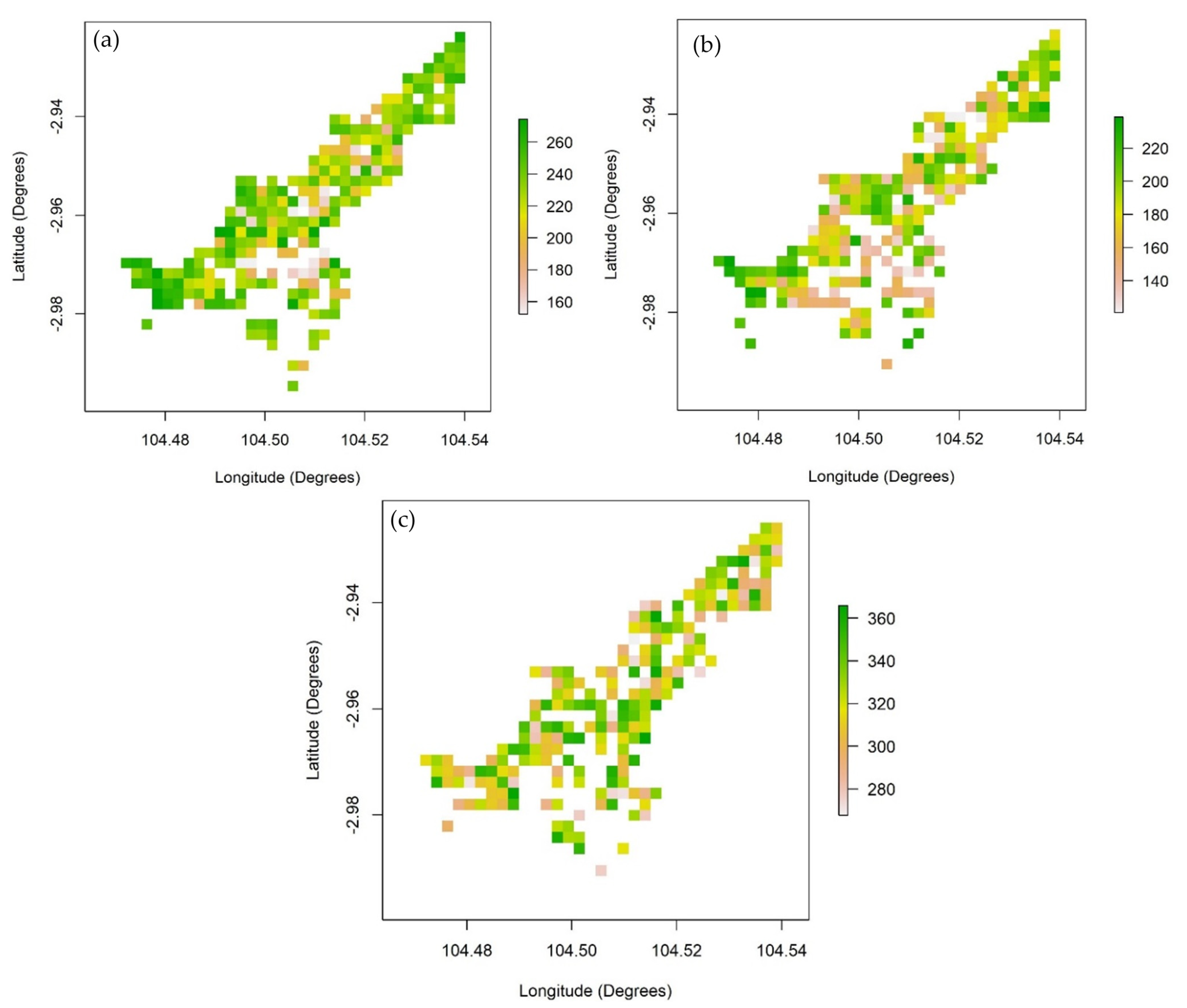
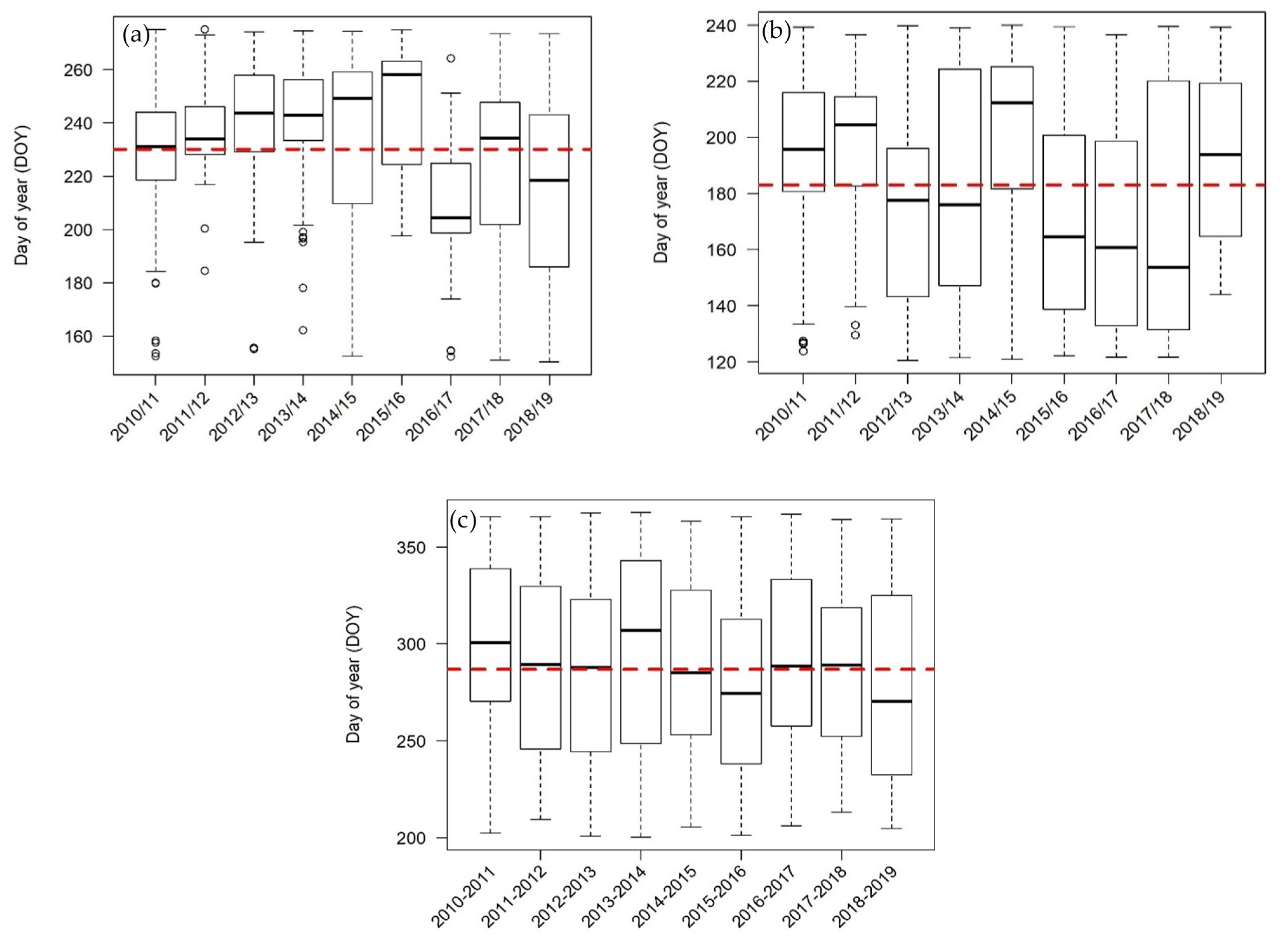
3.1. Phenological Characterisations

The spatial distributions of the phenological metrics SOS, EOS, and LOS over the study area were summarised from 2010 to 2019 based on the MODIS data used (Figure 6). The pixels represent the mean SOS/EOS/LOS for all nine seasons. The SOS date ranged widely from DOY 150 (end of May) to DOY 270 (end of September). The EOS date ranged from DOY 120 (end of April) to DOY 240 (end of August). The LOS value over the region ranged from 270 days to 365 days. Compared to LOS, SOS, and EOS dates had a more considerable variation. In general, there were quite similar spatial patterns between SOS and EOS throughout the study area. Earlier SOS date pixels have earlier EOS and vice versa for later dates pixels. This indicates that certain parts of the study area start to refoliate and defoliate earlier than others, a finding consistent with multiclonal planting.
The inter-annual variations of SOS and EOS for the study area during 2010 to 2019 are presented in Figure 7. In this figure, there were nine boxplots plotted for each phenological metric, indicating growing seasons from 2010/11 to 2018/19. There is no boxplot for growing season 2019/20 as the full cycle of this growing season was not complete. From the boxplots results, the overall mean of SOS and EOS was observed at DOY 230 and 185. Meanwhile the overall mean of LOS was found to be 318 days. Large differences in SOS (Figure 7a) and EOS (Figure 7b) boxplots are seen between years which may be expected to be driven by environmental factors. However, the LOS boxplot (Figure 7c) has all median lines overlapping with relatively small differences, indicating that LOS does not vary significantly between years and almost all parts of the study area experience a similar number of days per season.
Late SOS was observed in growing season 2014/15 and 2015/16, while early SOS was seen in 2016/17 and 2018/19. Noticeably late EOS was observed in 2011/12 and 2014/15, whereas early EOS was seen for three consecutive years from 2015/16 to 2017/18. Information from the literature and plantation information was gathered to identify the likely causes of these incidents.
We calculated the overall mean, standard deviation, variance, and dispersion index for the SOS/EOS/LOS data of each growing season (Table 1). The low standard deviation and variance values indicate minimal fluctuation in the LOS data. Unlike SOS and EOS, the LOS dispersion index was almost 0, making it a constant random variable. Due to this, further analyses were only conducted with the phenological metrics of SOS and EOS. On the other hand, SOS and EOS datasets have high standard deviation and variance values. However, both are still under-dispersed with dispersion index values less than 1.

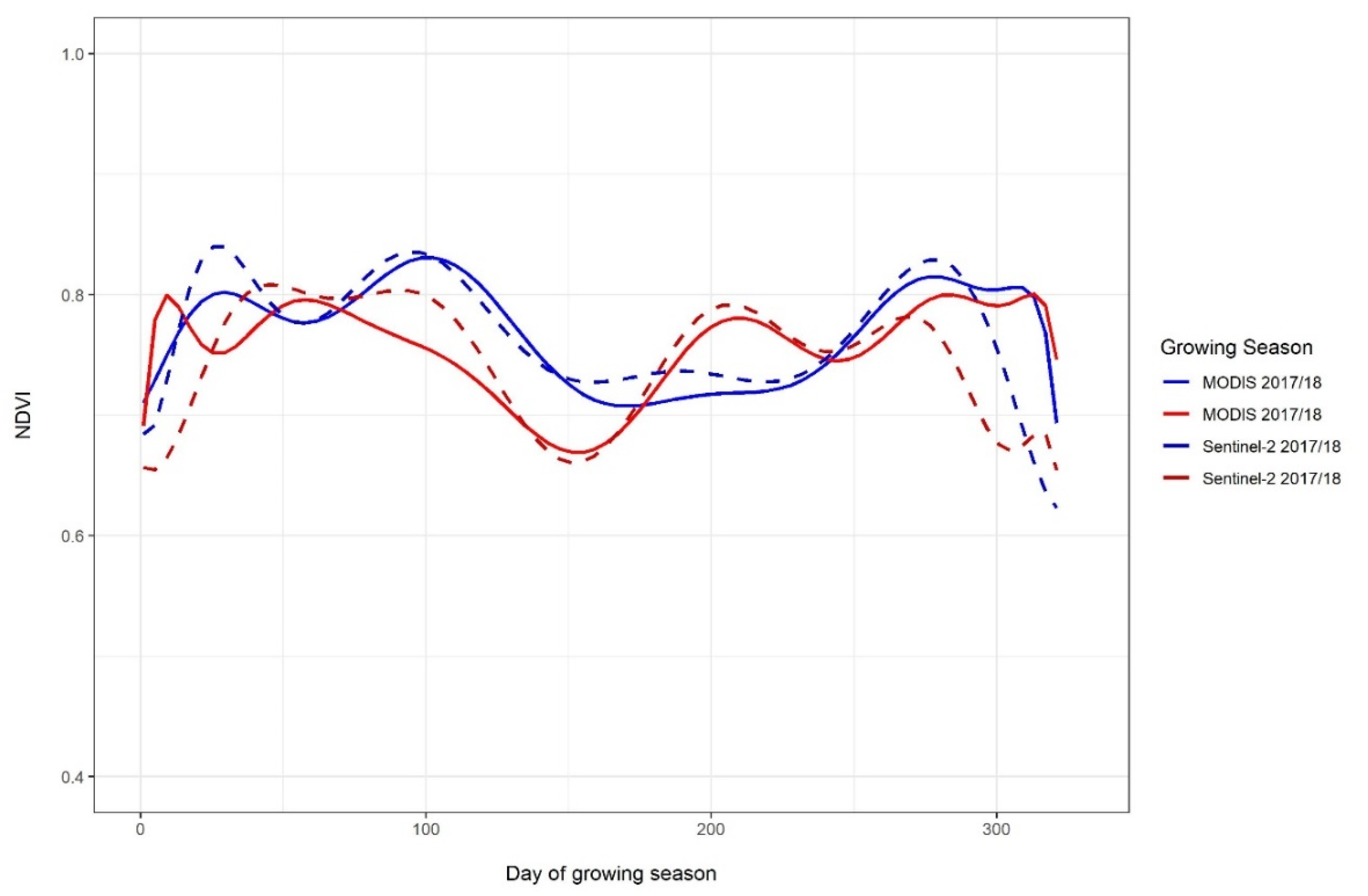
Validation of MODIS Phenological Data

The SOS and EOS determined using remote sensing were aligned with observed conditions on the ground. Rubber experts from the study area verified that the SOS and EOS dates detected from each season were within the expected range. In order to verify the accuracy of the SOS, EOS, and LOS data extracted from MODIS NDVI data, the same methodology was applied to Sentinel-2 NDVI data from 2017 to 2019. The SOS, EOS, and LOS average value of seasons 2017/18 and 2018/19, from both datasets, were then compared. The results based on the average value of all pixels are presented in Table 2.
The difference in SOS and EOS generated from both the satellites were less than ten days for both growing seasons and were not statistically significant following one-way ANOVA (p = 0.967). This indicates that the phenological metrics generated from MODIS data are comparable to the those extracted from Sentinel-2 data.

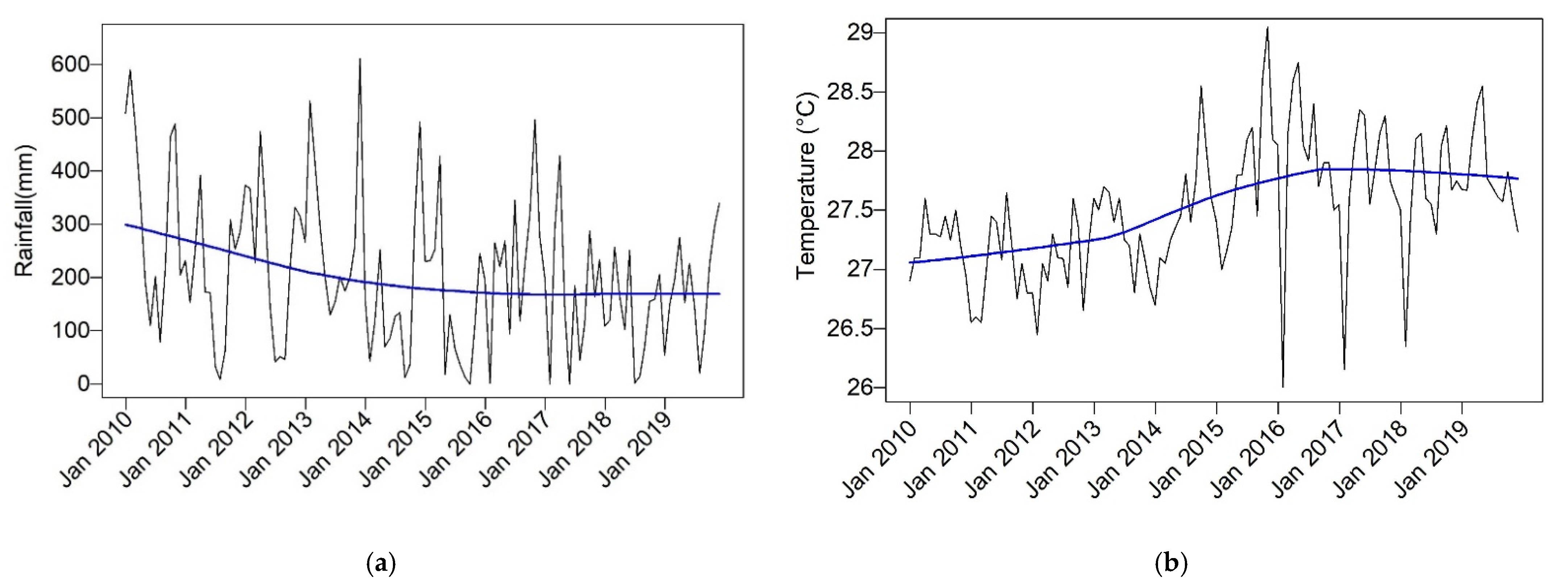
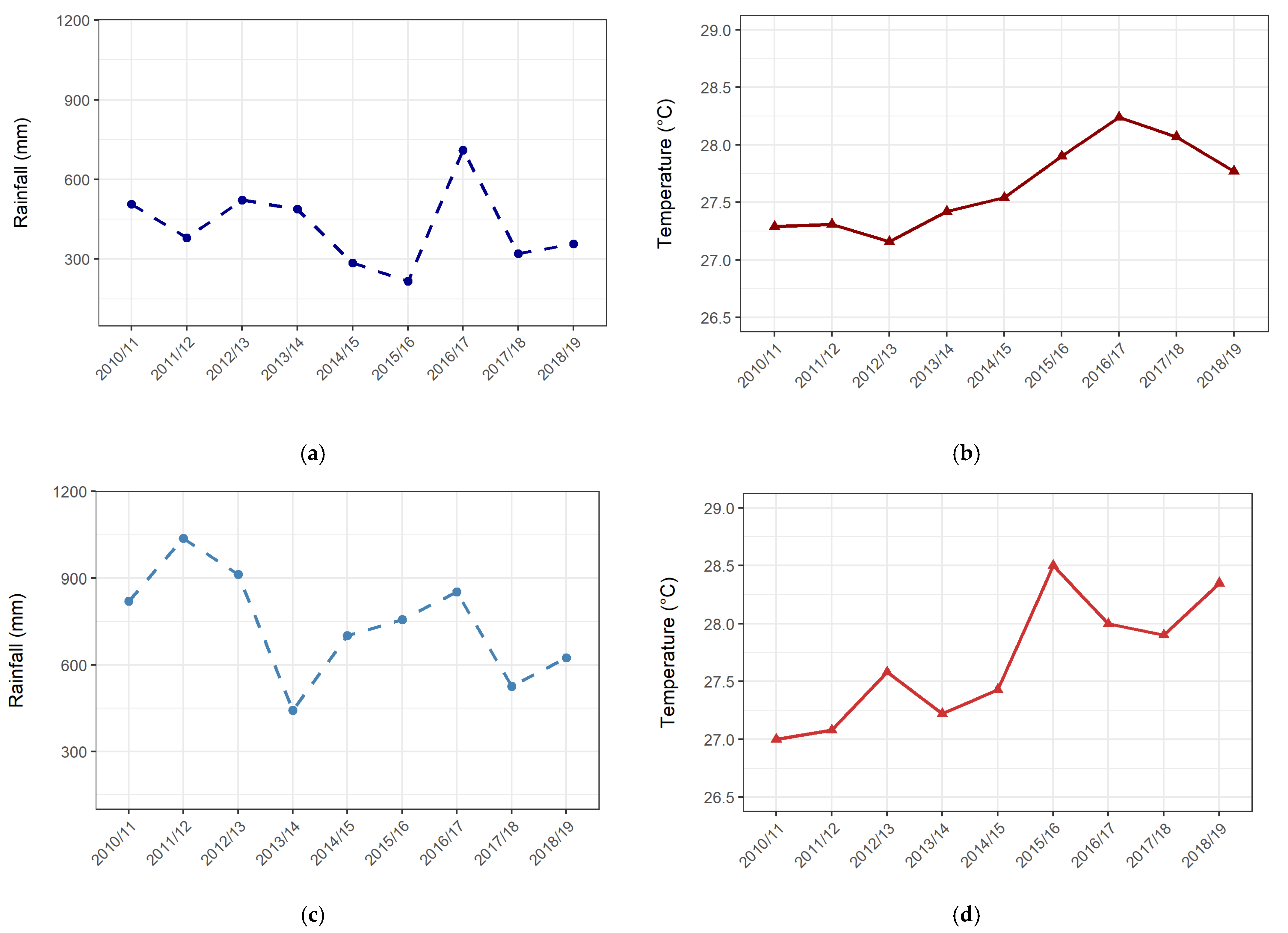
3.2. Climate Data Trend

We used the Mann–Kendall test and Sen’s slope estimator for detecting monotonic trends in rainfall and temperature. The total monthly rainfall and average monthly temperature data from 2010 to 2019 were used for this purpose. The data, including trend lines, were plotted in Figure 8. The trend line used for both plots in this figure is a Loess regression line, commonly used for smoothing a volatile time-series such as climate data.
From the Mann-Kendall test result, a statistically significant p-value (p < 0.05) was found for both climate data, indicating the presence of monotonic trend. The Tau values for rainfall and temperature are −0.162 and 0.387, respectively. The positive Tau value denotes an upward trend, while the negative value indicates a downward trend. These values showed that the study area experienced a decrease in monthly rainfall and an increase in monthly mean temperature over the study period. The Sen’s slope results confirmed the Tau values by giving an estimate of a total monthly rainfall data decrease of 0.93 mm and average monthly temperature increase of 0.008 °C, per month. The single change-point in a monthly rainfall and temperature series based on the Pettitt’s test was identified in December 2013 and June 2014, respectively.

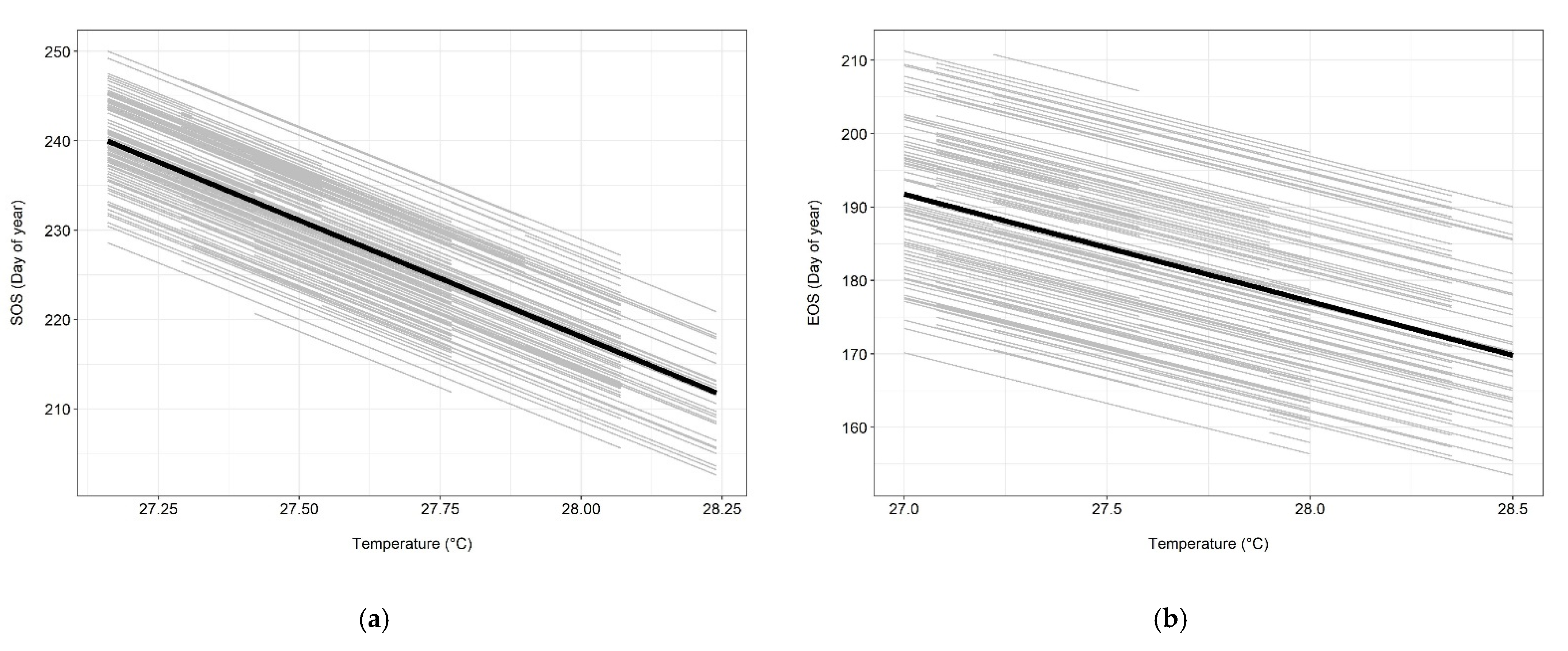
3.3. Relative Influence of Rainfall and Temperature on SOS/EOS

We investigated the relationship between SOS/EOS and pre-SOS/pre-EOS rainfall and temperature by developing the linear mixed models to evaluate the SOS/EOS response. The AIC values recorded for all competing model structures for SOS and EOS ranged from 6313.0 to 6382.2 and from 5436.1 to 5462.4, respectively. Based on AIC comparison of competing model structures, the random intercept mixed models of SOS and EOS with temperature as the sole significant predictor were identified to have the lowest value. This shows that temperature regulates the start and end of the rubber growing season. Table 3 shows the resulting model equations for SOS and EOS. The linear mixed model revealed a decreasing trend of SOS/EOS with an increase in temperature (Figure 9).
The results suggest that the random effect of pixel plays a role in influencing both SOS and EOS. All pixels in Figure 9 consistently showed a decreasing trend in SOS/EOS. This indicates that although there is rubber multiclonal planting, all clones in the study area respond similarly to temperature. In general, the level of SOS/EOS response to pre-SOS/EOS temperature were calculated to be −25.26 days/°C and −13.78 days/°C, respectively. These negative coefficients indicate that an increase in temperature advances the SOS/EOS dates, and vice versa.

4. Discussion

4.1. Phenological Metrics of SOS, EOS, and LOS

The main aim of this study was to evaluate the influence of rainfall and average temperature on rubber phenological metrics. We first extracted three important phenological metrics, SOS, EOS, and LOS, from the MODIS NDVI data. We computed the overall mean of SOS, EOS, and LOS for the study area on a pixel basis from these data. Both the SOS (DOY 150–270) and EOS (DOY 120–240) range falls within the normal range of wintering dates in South Sumatra, within the dry season. This indicates that the SOS and EOS are representative of defoliation and refoliation periods in the study area. The rubber defoliation and refoliation process occur during the dry season [79]. The spatial distribution map of mean SOS and EOS varies from pixel to pixel. This can be due to two reasons: (1) uneven distribution of mature plantations or trees age [80]; and (2) different rubber clones planted [81]. The year 2010 was chosen as the start of study duration because it is the year when most trees reached maturity in the study area. The plantations are said to reach maturity when 80% of total trees have a circumference over 45 cm [82] which means there is still a mixture of mature and immature trees on the ground. Additionally, immature trees are unlikely to experience wintering. This will alter the SOS/EOS dates to some extent. On the other hand, some clones are more sensitive to meteorological factors, which can impact the wintering period. For example, while comparing five rubber clones, Liyanage et al. [5] found that RRIM 600 and GT1 defoliated and refoliated one to two weeks earlier than clones Yunyan 277-5, Yunyan 34-4, and PR 107. These two clones also have shorter wintering periods compared to the other three clones. It is a common practice in rubber plantations to plant different clones and stagger the planting time [83]. This can explain the inter-variability illustrated in Figure 6.
We observed substantial fluctuations in SOS and EOS in specific years during the study period. Similar findings were reported by Zhai et al. [9]. Their study focused on the refoliation period from 2003 to 2011 using ground data. They found that the year 2005, 2009, and 2010 showed an early start of refoliation with rapid development, while 2008 also had an early start but slow growth. The other years (2003, 2004, 2006, 2007, and 2011) displayed a late onset of refoliation with rapid development. The fluctuations in SOS and EOS were also noticed in other croplands, such as in the salt marsh ecosystem. Shuvankar et al. [21] observed a delay in SOS for 2000, 2010, and 2013. They concluded that this could possibly be due to dieback, late spring, and hurricane Isaac. The salt marshes of southeast Los Angeles also experienced advances in EOS for 2005 and 2008, where storms were identified to have played a contributing role. The advancement and delay in both phenological metrics likely reflect environmental climatic anomalies or extreme weather events.
In our study, the SOS was found to have been delayed in 2014/15 and 2015/16. This could be attributed to the reduction in rainfall seen in both years based on the recorded climatic data. The 90-day pre-SOS rainfall accumulation recorded for these two periods was almost half of the 10-year average (see 90-day pre-SOS rainfall plot in Figure A1 in the Appendix A). In 2016/17 and 2018/19, there was an advancement in the SOS dates. It was most notable in 2016/17, where the SOS occurred almost 30 days earlier than the mean SOS date. This can possibly be due to high rainfall and temperature, as the rainfall accumulation recorded in this season was nearly double the average 90-day period before the SOS date (see 90-day preSOS rainfall plot in Figure A1 in the Appendix A). In studying vegetation phenology in Southeast Asia, Suepa et al. [84] concluded that rainfall could be the most dominant factor influencing phenological changes in this region, particularly on rainfed cropland. A study conducted on rubber trees has reported that high rainfall during the refoliation period delayed the entire leaf ageing process [9]. Meanwhile, the recorded temperature was the highest amongst all the seasons (see 90-day pre-SOS temperature plot in Figure A1 in the Appendix A). Zhai et al. [9] found that temperature was a significant climatic variable that influenced rubber phenology. The advancement in 2018/19 is thought to be associated with a rubber leaf disease outbreak, whose cause is under investigation. This outbreak in South Sumatra is reported to have begun in late 2017 [85]. The disease was evident until the present (2021), with high and low levels of severity. The year 2018 recorded high levels of disease severity and could thus have caused premature SOS. The NDVI plots of the growing season during the disease outbreak showed a drop in the value (see NDVI plot for 2018/19 and 2017/18 in Figure A2 in the Appendix A).
There were noticeable delays in EOS in 2011/12 and 2014/15. Based on the 90-day of pre-EOS, these two periods had high rainfall accumulation (see 90-day preEOS rainfall plot in Figure A1 in the Appendix A), causing wet conditions and fewer sunshine hours. Rubber is known to respond to sunlight duration, and reduced sunlight hours leads to a delay in the phenophase [5]. The advance in EOS can be seen in three consecutive years from 2015/16 to 2017/18. These advances can also be linked to the disease outbreak, which is believed to shorten the EOS period. Previous studies have also reported that fluctuations in phenological metrics can be caused by non-ecological factors such as oil spills [21] and soil moisture [64]. The EOS advance in 2017/18 could also be due to low rainfall accumulation during the dry season. A more pronounced dry season will shorten the defoliation period [81]. The standard deviation, variance, and dispersion index values have shown some fluctuation in SOS and EOS datasets. Meanwhile, there is no fluctuation seen in LOS. Generally, the rubber season in the study area commences around mid-August (DOY 230) and ends around early-July (DOY 183) in the following year. Each season spans an average of 318 days. This implies that rubber trees in the study area remain leafless for approximately 47 days (between 6 and 7 weeks). A defoliation period normally takes 2 to 3 weeks before new shoots emerge [86,87], whereas the refoliation period takes approximately 4 to 5 weeks [9]. In general, defoliation (EOS) and refoliation (SOS) is a sequential process that is typically one to two months apart [88].

Phenological Validation

The MODIS derived SOS, EOS, and LOS were validated with SOS, EOS, and LOS extracted from Sentinel NDVI data using the growing seasons of 2017/18 and 2018/19. ANOVA results confirmed a good agreement between phenological metrics derived from MODIS NDVI and Sentinel-2 NDVI. This is an indication that the MODIS derived phenological metrics are a reliable representation of rubber phenological events in the study area. Early SOS was seen in Sentinel-2 data for 2018/19 compared to MODIS. This was expected, as two studies have demonstrated that SOS for coarser-resolution image dataset is highly correlated to an early SOS identified in the fine-resolution image dataset [89,90]. The NDVI from these satellites indicated a similar pattern, with Sentinel-2 being more sensitive in capturing rubber canopy changes (see Figure A3 in the Appendix A). The study conducted by Yan Cheng et al. [68] has shown that fine-resolution data are better at retrieving phenological patterns, however due to limited data, we have used MODIS for the purpose of this study.
The existence of minor discrepancies in the two datasets can be explained by missing data due to the cloud presence and different pixel data representation, even though the same configuration was set in TIMESAT. Both datasets have different cloud cover percentages, and the data pixels in MODIS represents the combined maximum of the best 8-day observations, while Sentinel-2 data represents daily data taken on a particular date. Another factor influencing differences in the two datasets is the difference in the yearly image numbers of each data used in TIMESAT. There are 46 (at 8-day interval) and 36 (at 10-day interval) images per year used for MODIS and Sentinel-2, respectively. These three factors affect the smoothing process and the calculation of phenological metrics extracted in TIMESAT. In addition to this, non-vegetational effects such as soil-wetness [91], viewing geometry, and illumination conditions [92,93], and distorted signal under overcast conditions [94] may alter the received phenological signal and thus contribute to the observed data discrepancy.

4.2. Trend and Changes in Rainfall and Temperature

We tested the 10-year monthly rainfall and temperature data to investigate whether there is a trend in the time series data. The test proved that changes in rainfall and temperature have occurred during this period, but it is not known how this relates to periods further back in time. A significant shift in the central tendency of the rainfall and climate time series data were observed in December 2013 and June 2014, respectively. This is in line with the inter-annual variation data, where changes after these dates were seen to be notable compared to the period prior to that.

4.3. SOS/EOS Response to Rainfall and Temperature

Previous studies, such as Ren et al. [11], have used the regression coefficient from multiple linear regression between seasonal parameters and climatic variables to explain the relative influence of rainfall and temperature on the variability of SOS/EOS. In this study, we used the linear mixed model to analyse SOS/EOS response to rainfall and temperature. The mixed model has the advantage of producing estimates of both random and fixed effects, which allowed us to investigate the effects of climate factors while accounting for inter-pixel heterogeneity. Furthermore, it is not hindered by missing data [95]. The best-supported models demonstrate that temperature is a significant predictor of rubber phenology, being negatively related to SOS/EOS.
Despite the heterogeneity of the SOS/EOS values in the study area, a decreasing trend with an increasing temperature was identified across all pixels. This trend indicates an increase of 1 °C of temperature advanced the SOS/EOS by approximately 25 days and 14 days, respectively. Temperature is one of the main factors that affect the rate of plant development [96,97]. Higher temperatures accelerate phenological progression [98]. It can be explained by the fact that the temperature changes affect most biochemical processes of ectotherms, such as reaction kinetics, enzyme inactivation, and hormonal regulation [97]. This has been demonstrated by this study where SOS and EOS were seen to occur earlier with warmer temperatures.
In this study, the temperature was found to be a key factor in rubber phenology. However, when comparing the results to several crops and regions, the determinant factor of phenology varies considerably. Table 4 shows a comparison of the findings from other related studies. For example, two of the previous studies [99,100] conducted on forests found rainfall to be an influential factor in forest phenology, while another [101] showed both rainfall and temperature to be important factors.
The studies of phenology in Alpine regions [33,102], African savanna [104], European and South Korean vegetation [92,97] have similar findings to this study. More importantly, our result also agrees with previous studies carried out on rubber plantations. Two ground studies also discovered temperature as a critical driver of rubber phenology, either as the only factor [9] or with sunshine hour [5]. Priyadarshan [42] stated that both rainfall and temperature are important climatic factors for rubber phenology. However, he also mentioned that temperature was the most influential factor, particularly in rubber refoliation. The temperature is not only an important key indicator for rubber phenology but also for rubber yield. In their study, Ali et al. [106] discovered temperature to be the only significant predictor for rubber yield compared to other climatic parameters such as rainfall, relative humidity, and vapour pressure deficit.

5. Conclusions

Overall, this study demonstrates the ability to use remote sensing data to facilitate understanding of rubber phenology over a decade. The finding is strongly supported by several previous studies, including the one performed using ground data. The results also indicate that appropriate selection of data, good data fusion and proper phenological metrics extraction technique can provide enough information on phenological studies. These also minimise the adverse effects of missing data due to persistent clouds, which are common in rubber-producing countries. Combining MODIS Terra and Aqua at 250 m spatial resolution has enabled adequate data acquisition for phenological analysis. Although some fluctuations and inter-annual variability exist, these were caused by variability in rubber tree age and clones. Most SOS and EOS were within relevant timeframes, between July and August. Analysis of the results indicates that there was a significant downward trend detected in the rainfall data and a significant upward trend detected for temperature data. The mixed model analysis showed that temperature was the main factor in modulating rubber phenology.
In addition, this is the first study to demonstrate the use of multi-series remote sensing data to monitor rubber phenology. Although the study used moderate spatial resolution, it was shown to capture the annual dynamic growth of rubber plantations due to the large and homogenous planting area. This study provides a deeper understanding of how climate modulates rubber phenological metrics. Simultaneously, this information and insight are vital to developing effective control measures for rubber diseases, as well as for predicting rubber yields.

Author Contributions

Conceptualisation, F.A.A., I.S.A. and A.W.; methodology, F.A.A.; resources, T.R.F.; software, F.A.A. and M.I.A.; validation, I.S.A.; analysis, F.A.A.; writing—original draft preparation, F.A.A.; writing—review and editing, A.W., A.Y. and A.A.A.; supervision, I.S.A., A.Y. and A.A.A. All authors have read and agreed to the published version of the manuscript.

Funding

This research received no external funding.

Institutional Review Board Statement

Not applicable.

Informed Consent Statement

Not applicable.

Data Availability Statement

The MODIS and Sentinel-2 data are available from USGS EarthExplorer (https://earthexplorer.usgs.gov/ (accessed on 1 February 2020)). Other data used in this study are available from the corresponding author upon request.

Acknowledgments

We would like to thank Indonesian Rubber Research Institute for their excellent cooperation, valuable information, and assistance during data collection. We also thank expert reviewers for insightful contributions and suggestions. The first author acknowledges the Ministry of Higher Education Malaysia and University Malaysia Perlis for providing scholarship.

Conflicts of Interest

The authors declare no conflict of interest.

Appendix A

Figure A1. 90-day pre-season data for: (a) preSOS rainfall; (b) preSOS temperature; (c) preEOS rainfall; and (d) preSOS temperature.
Remotesensing 13 02932 g0a1
Figure A2. The NDVI trend line for all growing seasons from MODIS data.
Remotesensing 13 02932 g0a2
Figure A3. Comparison of NDVI trend line for growing seasons 2017/18 and 2018/19 for MODIS and Sentinel-2.
Remotesensing 13 02932 g0a3

References

  1. Lieth, H. Phenology and Seasonality Modeling; Springer Science+Business Media Verlag: Berlin, Germany, 1974; ISBN 9788578110796. [Google Scholar]
  2. Adole, T.; Dash, J.; Atkinson, P.M. A systematic review of vegetation phenology in Africa. Ecol. Inform. 2016, 34, 117–128. [Google Scholar] [CrossRef]
  3. IPCC. Climate Change Impacts, Adaptation, and Vulnerability. Contribution of Working Group II to the Fourth Assessment Report of the Intergovernmental Panel on Climate Change; IPCC: Geneva, Switzerland, 2007. [Google Scholar]
  4. Rosenzweig, C.; Casassa, G.; Karoly, D.J.; Imeson, A.; Liu, C.; Menzel, A.; Rawlins, S.; Root, T.L.; Seguin, B.; Tryjanowski, P. Assessment of observed changes and responses in natural and managed systems. In Contribution of Working Group II to the Fourth Assessment Report of the Intergovernmental Panel on Climate Change; Cambridge University Press: Cambridge, UK, 2007; pp. 79–131. ISBN 9780521880107. [Google Scholar]
  5. Liyanage, K.K.; Khan, S.; Ranjitkar, S.; Yu, H.; Xu, J.; Brooks, S.; Beckschäfer, P.; Hyde, K.D. Evaluation of key meteorological determinants of wintering and flowering patterns of five rubber clones in Xishuangbanna, Yunnan, China. Int. J. Biometeorol. 2019, 63, 617–625. [Google Scholar] [CrossRef]
  6. Workie, T.G.; Debella, H.J. Climate change and its effects on vegetation phenology across ecoregions of Ethiopia. Glob. Ecol. Conserv. 2018, 13, e00366. [Google Scholar] [CrossRef]
  7. Vitasse, Y.; Delzon, S.; Dufrêne, E.; Pontailler, J.Y.; Louvet, J.M.; Kremer, A.; Michalet, R. Leaf phenology sensitivity to temperature in European trees: Do within-species populations exhibit similar responses? Agric. For. Meteorol. 2009, 149, 735–744. [Google Scholar] [CrossRef]
  8. Sekhwela, M.B.M.; Yates, D.J. A phenological study of dominant acacia tree species in areas with different rainfall regimes in the Kalahari of Botswana. J. Arid Environ. 2007, 70, 1–17. [Google Scholar] [CrossRef]
  9. Zhai, D.-L.; Yu, H.; Chen, S.C.; Ranjitkar, S.; Xu, J. Responses of rubber leaf phenology to climatic variations in Southwest China. Int. J. Biometeorol. 2017, 63, 607–616. [Google Scholar] [CrossRef]
  10. Broich, M.; Huete, A.; Tulbure, M.G.; Ma, X.; Xin, Q.; Paget, M.; Restrepo-Coupe, N.; Davies, K.; Devadas, R.; Held, A. Land surface phenological response to decadal climate variability across Australia using satellite remote sensing. Biogeosciences 2014, 11, 5181–5198. [Google Scholar] [CrossRef] [Green Version]
  11. Ren, S.; Yi, S.; Peichl, M.; Wang, X. Diverse responses of vegetation phenology to climate change in different Grasslands in Inner Mongolia during 2000-2016. Remote Sens. 2017, 10, 17. [Google Scholar] [CrossRef] [Green Version]
  12. Lin, Y.; Zhang, Y.; Zhao, W.; Dong, Y.; Fei, X.; Song, Q.; Sha, L.; Wang, S.; Grace, J. Pattern and driving factor of intense defoliation of rubber plantations in SW China. Ecol. Indic. 2018, 94, 104–116. [Google Scholar] [CrossRef]
  13. Zeng, L.; Wardlow, B.D.; Xiang, D.; Hu, S.; Li, D. A review of vegetation phenological metrics extraction using time-series, multispectral satellite data. Remote Sens. Environ. 2020, 237, 111511. [Google Scholar] [CrossRef]
  14. Jinji, P.; Xin, Z.; Yangxian, Q.; Yixian, X.; Huiqiang, Z.; He, Z. First record of Corynespora leaf fall disease of Hevea rubber tree in China. Australas. Plant Dis. Notes 2007, 2, 35. [Google Scholar] [CrossRef] [Green Version]
  15. Brown, M.E.; de Beurs, K.M.; Marshall, M. Global phenological response to climate change in crop areas using satellite remote sensing of vegetation, humidity and temperature over 26 years. Remote Sens. Environ. 2012, 126, 174–183. [Google Scholar] [CrossRef]
  16. Gong, Z.; Kawamura, K.; Ishikawa, N.; Goto, M.; Wulan, T.; Alateng, D.; Yin, T.; Ito, Y. MODIS normalized difference vegetation index (NDVI) and vegetation phenology dynamics in the Inner Mongolia grassland. Solid Earth 2015, 6, 1185–1194. [Google Scholar] [CrossRef] [Green Version]
  17. Yu, L.; Liu, T.; Bu, K.; Yan, F.; Yang, J.; Chang, L.; Zhang, S. Monitoring the long term vegetation phenology change in Northeast China from 1982 to 2015. Sci. Rep. 2017, 7, 14770. [Google Scholar] [CrossRef] [Green Version]
  18. Weber, M.; Hao, D.; Asrar, G.R.; Zhou, Y.; Li, X.; Chen, M. Exploring the use of DSCOVR/EPIC satellite observations to monitor vegetation phenology. Remote Sens. 2020, 12, 2384. [Google Scholar] [CrossRef]
  19. Wheeler, K.; Dietze, M. Improving the monitoring of deciduous broadleaf phenology using the Geostationary Operational Environmental Satellite (GOES) 16 and 17. Biogeosci. Discuss. 2020, 18, 1971–1985. [Google Scholar] [CrossRef]
  20. Cho, M.A.; Ramoelo, A.; Dziba, L. Response of land surface phenology to variation in tree cover during green-up and senescence periods in the semi-arid savanna of Southern Africa. Remote Sens. 2017, 9, 689. [Google Scholar] [CrossRef] [Green Version]
  21. Ghosh, S.; Mishra, D.R. Analyzing the Long-Term Phenological Trends of Salt Marsh Ecosystem across Coastal LOUISIANA. Remote Sens. 2017, 9, 1340. [Google Scholar] [CrossRef] [Green Version]
  22. Qiu, T.; Song, C.; Li, J. Deriving annual double-season cropland phenology using landsat imagery. Remote Sens. 2020, 12, 3275. [Google Scholar] [CrossRef]
  23. Schwieder, M.; Leitão, P.J.; Pinto, J.R.R.; Teixeira, A.M.C.; Pedroni, F.; Sanchez, M.; Bustamante, M.M.; Hostert, P. Landsat phenological metrics and their relation to aboveground carbon in the Brazilian Savanna. Carbon Balance Manag. 2018, 13, 1–15. [Google Scholar] [CrossRef] [Green Version]
  24. White, K.; Pontius, J.; Schaberg, P. Remote sensing of spring phenology in northeastern forests: A comparison of methods, field metrics and sources of uncertainty. Remote Sens. Environ. 2014, 148, 97–107. [Google Scholar] [CrossRef]
  25. Merrick, T.; Pau, S.; Jorge, M.L.S.P.; Silva, T.S.F.; Bennartz, R. Spatiotemporal patterns and phenology of tropical vegetation solar-induced chlorophyll fluorescence across brazilian biomes using satellite observations. Remote Sens. 2019, 11, 1746. [Google Scholar] [CrossRef] [Green Version]
  26. Lu, X.; Liu, Z.; Zhou, Y.; Liu, Y.; An, S.; Tang, J. Comparison of phenology estimated from reflectance-based indices and solar-induced chlorophyll fluorescence (SIF) observations in a temperate forest using GPP-based phenology as the standard. Remote Sens. 2018, 10, 932. [Google Scholar] [CrossRef] [Green Version]
  27. Jeong, S.J.; Schimel, D.; Frankenberg, C.; Drewry, D.T.; Fisher, J.B.; Verma, M.; Berry, J.A.; Lee, J.E.; Joiner, J. Application of satellite solar-induced chlorophyll fluorescence to understanding large-scale variations in vegetation phenology and function over northern high latitude forests. Remote Sens. Environ. 2017, 190, 178–187. [Google Scholar] [CrossRef]
  28. Pan, Z.; Huang, J.; Zhou, Q.; Wang, L.; Cheng, Y.; Zhang, H.; Blackburn, G.A.; Yan, J.; Liu, J. Mapping crop phenology using NDVI time-series derived from HJ-1 A/B data. Int. J. Appl. Earth Obs. Geoinf. 2015, 34, 188–197. [Google Scholar] [CrossRef] [Green Version]
  29. Wu, C.; Peng, D.; Soudani, K.; Siebicke, L.; Gough, C.M.; Arain, M.A.; Bohrer, G.; Lafleur, P.M.; Peichl, M.; Gonsamo, A.; et al. Land surface phenology derived from normalized difference vegetation index (NDVI) at global FLUXNET sites. Agric. For. Meteorol. 2017, 233, 171–182. [Google Scholar] [CrossRef]
  30. Shen, M.; Zhang, G.; Cong, N.; Wang, S.; Kong, W.; Piao, S. Increasing altitudinal gradient of spring vegetation phenology during the last decade on the Qinghai-Tibetan Plateau. Agric. For. Meteorol. 2014, 189–190, 71–80. [Google Scholar] [CrossRef]
  31. Zhang, X.; Friedl, M.A.; Schaaf, C.B.; Strahler, A.H. Climate controls on vegetation phenological patterns in northern mid- and high latitudes inferred from MODIS data. Glob. Chang. Biol. 2004, 10, 1133–1145. [Google Scholar] [CrossRef]
  32. Wang, H.; Tetzlaff, D.; Buttle, J.; Carey, S.K.; Laudon, H.; McNamara, J.P.; Spence, C.; Soulsby, C. Climate-phenology-hydrology interactions in northern high latitudes: Assessing the value of remote sensing data in catchment ecohydrological studies. Sci. Total Environ. 2019, 656, 19–28. [Google Scholar] [CrossRef] [Green Version]
  33. Busetto, L.; Colombo, R.; Migliavacca, M.; Cremonese, E.; Meroni, M.; Galvagno, M.; Rossini, M.; Siniscalco, C.; Morra Di Cella, U.; Pari, E. Remote sensing of larch phenological cycle and analysis of relationships with climate in the Alpine region. Glob. Chang. Biol. 2010, 16, 2504–2517. [Google Scholar] [CrossRef]
  34. Ulsig, L.; Nichol, C.J.; Huemmrich, K.F.; Landis, D.R.; Middleton, E.M.; Lyapustin, A.I.; Mammarella, I.; Levula, J.; Porcar-Castell, A. Detecting inter-annual variations in the phenology of evergreen conifers using long-term MODIS vegetation index time series. Remote Sens. 2017, 9, 49. [Google Scholar] [CrossRef] [Green Version]
  35. Thompson, J.A.; Paull, D.J. Assessing spatial and temporal patterns in land surface phenology for the Australian Alps (2000–2014). Remote Sens. Environ. 2017, 199, 1–13. [Google Scholar] [CrossRef]
  36. Kou, W.; Dong, J.; Xiao, X.; Hernandez, A.J.; Qin, Y.; Zhang, G.; Chen, B.; Lu, N.; Doughty, R. Expansion dynamics of deciduous rubber plantations in Xishuangbanna, China during 2000–2010. GIScience Remote Sens. 2018, 55, 905–925. [Google Scholar] [CrossRef]
  37. Zhai, D.; Dong, J.; Cadisch, G.; Wang, M.; Kou, W.; Xu, J.; Xiao, X.; Abbas, S. Comparison of pixel- and object-based approaches in phenology-based rubber plantation mapping in fragmented landscapes. Remote Sens. 2018, 10, 44. [Google Scholar] [CrossRef] [Green Version]
  38. Azizan, F.A.; Kiloes, A.M.; Astuti, I.S.; Abdul Aziz, A. Application of Optical Remote Sensing in Rubber Plantations: A Systematic Review. Remote Sens. 2021, 13, 429. [Google Scholar] [CrossRef]
  39. Fan, H.; Fu, X.; Zhang, Z.; Wu, Q. Phenology-based vegetation index differencing for mapping of rubber plantations using landsat OLI data. Remote Sens. 2015, 7, 6041–6058. [Google Scholar] [CrossRef] [Green Version]
  40. Li, Y.-Y.; Zhang, J.; Liu, C.-L.; Yang, X.-C.; Li, J. Research on Extraction and Spatial-Temporal Expansion of Rubber Forest in Five Provinces of Northern Laos Based on Multi-source Remote Sensing. For. Res. 2017, 30, 709–717. [Google Scholar] [CrossRef]
  41. Golbon, R.; Cotter, M.; Sauerborn, J. Climate change impact assessment on the potential rubber cultivating area in the Greater Mekong Subregion. Environ. Res. Lett. 2018, 13. [Google Scholar] [CrossRef]
  42. Priyadarshan, P.M. Biology of Hevea Rubber; Springer International Publishing AG: Cham, Switzerland, 2017; ISBN 9783319545066. [Google Scholar]
  43. Zapata-Gallego, N.T.; Álvarez-Láinez, M.L. Effect of the Phenological Stage in the Natural Rubber Latex Properties. J. Polym. Environ. 2019, 27, 364–371. [Google Scholar] [CrossRef]
  44. Sub Directorate of Estate Crops Statistics. Indonesian Rubber Statistics 2018; BPS–Statistics Indonesia: Central Jakarta, Indonesia, 2018.
  45. Sanjeeva Rao, P.; Saraswathyamma, C.K.; Sethuraj, M.R. Studies on the relationship between yield and meteorological parameters of para rubber tree (Hevea brasiliensis). Agric. For. Meteorol. 1998, 90, 235–245. [Google Scholar] [CrossRef]
  46. Schaaf, C.B.; Gao, F.; Strahler, A.H.; Lucht, W.; Li, X.; Tsang, T.; Strugnell, N.C.; Zhang, X.; Jin, Y.; Muller, J.; et al. First operational BRDF, albedo nadir reflectance products from MODIS. Remote Sens. Environ. 2002, 83, 135–148. [Google Scholar] [CrossRef] [Green Version]
  47. Leinenkugel, P.; Kuenzer, C.; Dech, S. Comparison and enhancement of MODIS cloud mask products for Southeast Asia. Int. J. Remote Sens. 2013, 34, 2730–2748. [Google Scholar] [CrossRef]
  48. Wang, S.; Lu, X.; Cheng, X.; Li, X.; Peichl, M. Limitations and Challenges of MODIS-Derived Phenological Metrics Across Different Landscapes in Pan-Arctic Regions. Remote Sens. 2018, 10, 1784. [Google Scholar] [CrossRef] [Green Version]
  49. Gallo, K.; Ji, L.; Reed, B.; Eidenshink, J.; Dwyer, J. Multi-platform comparisons of MODIS and AVHRR normalized difference vegetation index data. Remote Sens. Environ. 2005, 99, 221–231. [Google Scholar] [CrossRef] [Green Version]
  50. Wang, J.; Guo, N.; Wang, X.; Yang, J. Comparisons of normalized difference vegetation index from MODIS Terra and Aqua data in northwestern China. Int. Geosci. Remote Sens. Symp. 2007, 3390–3393. [Google Scholar] [CrossRef]
  51. Leinenkugel, P.; Kuenzer, C.; Oppelt, N.; Dech, S. Characterisation of land surface phenology and land cover based on moderate resolution satellite data in cloud prone areas-A novel product for the Mekong Basin. Remote Sens. Environ. 2013, 136, 180–198. [Google Scholar] [CrossRef]
  52. Qiao, D.; Wang, N. Relationship between winter snow cover dynamics, climate and spring grassland vegetation phenology in inner Mongolia, China. ISPRS Int. J. Geo-Inf. 2019, 8, 42. [Google Scholar] [CrossRef] [Green Version]
  53. Heumann, B.W.; Seaquist, J.W.; Eklundh, L.; Jönsson, P. AVHRR derived phenological change in the Sahel and Soudan, Africa, 1982–2005. Remote Sens. Environ. 2007, 108, 385–392. [Google Scholar] [CrossRef]
  54. Rouse, J.W.; Haas, R.H.; Schell, J.A.; Deering, D.W. Monitoring the Vernal Advancement and Retrogradation (Green Wave Effect) of Natural Vegetation; Remote Sensing Center Texas A&M University: College Station, TX, USA, 1973. [Google Scholar]
  55. Holben, B.N. Characteristics of maximum-value composite images from temporal AVHRR data. Int. J. Remote Sens. 1986, 7, 1417–1434. [Google Scholar] [CrossRef]
  56. Eklundh, L.; Jönsson, P. TIMESAT: A software package for time-series processing and assessment of vegetation dynamics. In Remote Sensing Time Series: Revealing Land Surface Dynamics; Kuenzer, C., Wagnerm, W., Dech, S., Eds.; Springer: Cham, Switzerland, 2015; pp. 141–158. ISBN 9783319159669. [Google Scholar]
  57. Hird, J.N.; McDermid, G.J. Noise reduction of NDVI time series: An empirical comparison of selected techniques. Remote Sens. Environ. 2009, 113, 248–258. [Google Scholar] [CrossRef]
  58. Wang, Y.; Xue, Z.; Chen, J.; Chen, G. Spatio-temporal analysis of phenology in Yangtze River Delta based on MODIS NDVI time series from 2001 to 2015. Front. Earth Sci. 2019, 13, 92–110. [Google Scholar] [CrossRef]
  59. Jayawardhana, W.G.N.N.; Chathurange, V.M.I. Extraction of Agricultural Phenological Parameters of Sri Lanka Using MODIS, NDVI Time Series Data. Procedia Food Sci. 2016, 6, 235–241. [Google Scholar] [CrossRef] [Green Version]
  60. de Castro, A.I.; Six, J.; Plant, R.E.; Peña, J.M. Mapping crop calendar events and phenology-related metrics at the parcel level by object-based image analysis (OBIA) of MODIS-NDVI time-series: A case study in central California. Remote Sens. 2018, 10, 1745. [Google Scholar] [CrossRef] [Green Version]
  61. Stanimirova, R.; Cai, Z.; Melaas, E.K.; Gray, J.M.; Eklundh, L.; Jönsson, P.; Friedl, M.A. An Empirical Assessment of the MODIS Land Cover Dynamics and TIMESAT Land Surface Phenology Algorithms. Remote Sens. 2019, 11, 2201. [Google Scholar] [CrossRef] [Green Version]
  62. Cai, Z.; Jönsson, P.; Jin, H.; Eklundh, L. Performance of smoothing methods for reconstructing NDVI time-series and estimating vegetation phenology from MODIS data. Remote Sens. 2017, 9, 1271. [Google Scholar] [CrossRef] [Green Version]
  63. Tan, B.; Morisette, J.; Wolfe, R.; Esaias, W.; Gao, F.; Ederer, G.; Nightingale, J.; Nickeson, J.E.; Ma, P.; Pedely, J. Modis Vegetation Phenology Metrics Estimated With an Enhanced Timesat Algorithm. IEEE J. Sel. Top. Appl. Earth Obs. Remote Sens. 2011, 4, 361–371. [Google Scholar] [CrossRef]
  64. Wang, J.; Zhou, T.; Peng, P. Phenology response to climatic dynamic across China’s grasslands from 1985 to 2010. ISPRS Int. J. Geo-Inf. 2018, 7, 290. [Google Scholar] [CrossRef] [Green Version]
  65. Wang, X.; Xiao, J.; Li, X.; Cheng, G.; Ma, M.; Zhu, G.; Altaf Arain, M.; Andrew Black, T.; Jassal, R.S. No trends in spring and autumn phenology during the global warming hiatus. Nat. Commun. 2019, 10, 2389. [Google Scholar] [CrossRef]
  66. Richardson, A.D.; Hufkens, K.; Milliman, T.; Frolking, S. Intercomparison of phenological transition dates derived from the PhenoCam Dataset V1.0 and MODIS satellite remote sensing. Sci. Rep. 2018, 8, 5679. [Google Scholar] [CrossRef] [Green Version]
  67. Bórnez, K.; Richardson, A.D.; Verger, A.; Descals, A.; Peñuelas, J. Evaluation of VEGETATION and PROBA-V phenology using phenocam and eddy covariance data. Remote Sens. 2020, 12, 3077. [Google Scholar] [CrossRef]
  68. Cheng, Y.; Vrieling, A.; Fava, F.; Meroni, M.; Marshall, M.; Gachoki, S. Phenology of short vegetation cycles in a Kenyan rangeland from PlanetScope and Sentinel-2. Remote Sens. Environ. 2020, 248, 112004. [Google Scholar] [CrossRef]
  69. Hufkens, K.; Melaas, E.K.; Mann, M.L.; Foster, T.; Ceballos, F.; Robles, M.; Kramer, B. Monitoring crop phenology using a smartphone based near-surface remote sensing approach. Agric. For. Meteorol. 2019, 265, 327–337. [Google Scholar] [CrossRef]
  70. He, Y.; Wang, A.; Huang, H. The trend of natural illuminance levels in 14 Chinese cities in the past 50 years. Energy Sustain. Soc. 2013, 3, 22. [Google Scholar] [CrossRef] [Green Version]
  71. Grafen, A.; Hails, R. Modern Statistics for the Life Sciences; Oxford University Press: Oxford, NY, USA, 2002; ISBN 8436817117. [Google Scholar]
  72. R Core Team. R: A Language and Environment for Statistical Computing; R Foundation for Statistical Computing: Vienna, Austria, 2017. [Google Scholar]
  73. Hijmans, R.J. Raster: Geographic Data Analysis and Modeling; R Package Version 3.4-10; 2021; Available online: https://cran.r-project.org/web/packages/raster/index.html (accessed on 1 July 2020).
  74. Bivand, R.; Keitt, T.; Rowlingson, B. Rgdal: Bindings for the “Geospatial” Data Abstraction Library; R Package Version 1.5-23; 2021; Available online: https://cran.r-project.org/web/packages/rgdal/index.html (accessed on 1 July 2020).
  75. Pebesma, E.J.; Bivand, R.S. Classes and methods for spatial data in R. R News 2005, 5, 9–13. [Google Scholar]
  76. Wickham, H.; Averick, M.; Bryan, J.; Chang, W.; McGowan, L.D.; François, R.; Grolemund, G.; Hayes, A.; Henry, L.; Hester, J.; et al. Welcome to the tidyverse. J. Open Source Softw. 2019, 4, 1686. [Google Scholar] [CrossRef]
  77. Pohlert, T. Trend: Non-Parametric Trend Tests and Change-Point Detection; R Package Version 1.1.4; 2020; Available online: https://cran.r-project.org/web/packages/trend/index.html (accessed on 15 July 2020).
  78. Bates, D.; Mächler, M.; Bolker, B.M.; Walker, S.C. Fitting linear mixed-effects models using lme4. J. Stat. Softw. 2015, 67. [Google Scholar] [CrossRef]
  79. Guardiola-Claramonte, M.; Troch, P.A.; Ziegler, A.D.; Giambelluca, T.W.; Vogler, J.B.; Nullet, M.A. Local hydrologic effects of introducing non-native vegetation in a tropical catchment. Ecohydrology 2008, 1, 13–22. [Google Scholar] [CrossRef]
  80. de Liyanage, A.S. Influence of Some Factors on the Pattern of Wintering and on the Incidence of Oidium Leaf Fall in Clone PB 86. J. Rubber Res. Inst. Sri Lanka 1976, 53, 31–38. [Google Scholar]
  81. Carr, M.K.V. The water relations of rubber (hevea brasiliensis): A review. Exp. Agric. 2012, 48, 176–193. [Google Scholar] [CrossRef]
  82. Moreira, A.; Moraes, L.A.C.; Cordeiro, E.R.; Fageria, N.K. Evaluation of Rubber Tree Crown Clones for Yield and Magnesium Use Efficiency in a Xanthic Ferralsol. J. Plant. Nutr. 2014, 37, 1171–1186. [Google Scholar] [CrossRef]
  83. Varghese, Y.A.; Mercykutty, V.C.; Panikkar, A.O.N.; George, P.J.; Sethuraj, M.R. Concept of clone blends: Monoculture vs. multiclone planting. Rubber Board Bull. 1990, 26, 13–19. [Google Scholar]
  84. Suepa, T.; Qi, J.; Lawawirojwong, S.; Messina, J.P. Understanding spatio-temporal variation of vegetation phenology and rainfall seasonality in the monsoon Southeast Asia. Environ. Res. 2016, 147, 621–629. [Google Scholar] [CrossRef] [Green Version]
  85. Association of Natural Rubber Producing Countries (ANRPC). Natural Rubber Trends and Statistics; Kuala Lumpur; ANRPC: Kuala Lumpur, Malaysia, 2020; Volume 12. [Google Scholar]
  86. Righi, C.A.; Bernardes, M.S. The potential for increasing rubber production by matching tapping intensity to leaf area index. Agrofor. Syst. 2008, 72, 1–13. [Google Scholar] [CrossRef]
  87. Moraes, V.H.F. Rubber. In Ecophysiology of Tropical Crops; Alvim, d.P.T., Kozlowski, T.T., Eds.; Academic Press: New York, NY, USA, 1977; ISBN 0120556502. [Google Scholar]
  88. Rao, S.B. Avoiding secondary leaf fall disease of rubber by chemical defoliation in nigeria. Pans Pest. Artic. News Summ. 1971, 17, 461–463. [Google Scholar] [CrossRef]
  89. Vrieling, A.; Skidmore, A.K.; Wang, T.; Meroni, M.; Ens, B.J.; Oosterbeek, K.; O’Connor, B.; Darvishzadeh, R.; Heurich, M.; Shepherd, A.; et al. Spatially detailed retrievals of spring phenology from single-season high-resolution image time series. Int. J. Appl. Earth Obs. Geoinf. 2017, 59, 19–30. [Google Scholar] [CrossRef]
  90. Zhang, X.; Wang, J.; Gao, F.; Liu, Y.; Schaaf, C.; Friedl, M.; Yu, Y.; Jayavelu, S.; Gray, J.; Liu, L.; et al. Exploration of scaling effects on coarse resolution land surface phenology. Remote Sens. Environ. 2017, 190, 318–330. [Google Scholar] [CrossRef] [Green Version]
  91. White, M.A.; de Beurs, K.M.; Didan, K.; Inouye, D.W.; Richardson, A.D.; Jensen, O.P.; O’Keefe, J.; Zhang, G.; Nemani, R.R.; van Leeuwen, W.J.D.; et al. Intercomparison, interpretation, and assessment of spring phenology in North America estimated from remote sensing for 1982–2006. Glob. Chang. Biol. 2009, 15, 2335–2359. [Google Scholar] [CrossRef]
  92. Stöckli, R.; Vidale, P.L. European plant phenology and climate as seen in a 20-year AVHRR land-surface parameter dataset. Int. J. Remote Sens. 2004, 25, 3303–3330. [Google Scholar] [CrossRef]
  93. Eklundh, L.; Jin, H.; Schubert, P.; Guzinski, R.; Heliasz, M. An optical sensor network for vegetation phenology monitoring and satellite data calibration. Sensors 2011, 11, 7678–7709. [Google Scholar] [CrossRef]
  94. Lange, M.; Dechant, B.; Rebmann, C.; Vohland, M.; Cuntz, M.; Doktor, D. Validating MODIS and sentinel-2 NDVI products at a temperate deciduous forest site using two independent ground-based sensors. Sensors 2017, 17, 1855. [Google Scholar] [CrossRef] [Green Version]
  95. Wang, Z.; Goonewardene, L.A. The use of MIXED models in the analysis of animal experiments with repeated measures data. Can. J. Anim. Sci. 2004, 84, 1–11. [Google Scholar] [CrossRef]
  96. Hatfield, J.L.; Prueger, J.H. Temperature extremes: Effect on plant growth and development. Weather Clim. Extrem. 2015, 10, 4–10. [Google Scholar] [CrossRef] [Green Version]
  97. Lee, H.K.; Lee, S.J.; Kim, M.K.; Lee, S.D. Prediction of Plant Phenological Shift under Climate Change in South Korea. Sustainabilty 2020, 12, 9276. [Google Scholar] [CrossRef]
  98. Prevéy, J.; Vellend, M.; Rüger, N.; Hollister, R.D.; Bjorkman, A.D.; Myers-Smith, I.H.; Elmendorf, S.C.; Clark, K.; Cooper, E.J.; Elberling, B.; et al. Greater temperature sensitivity of plant phenology at colder sites: Implications for convergence across northern latitudes. Glob. Chang. Biol. 2017, 23, 2660–2671. [Google Scholar] [CrossRef] [Green Version]
  99. Borchert, R. Responses of tropical trees to rainfall seasonality and its long-term changes. In Potential Impacts of Climate Change on Tropical Forest Ecosystems; Markham, A., Ed.; Springer: Berlin, Germany, 1998; pp. 241–253. ISBN 9781626239777. [Google Scholar]
  100. Eamus, D.; Prior, L. Ecophysiology of trees of seasonally dry tropics: Comparisons among phenologies. Adv. Ecol. Res. 2001, 32, 113–197. [Google Scholar] [CrossRef]
  101. Yu, X.; Wang, Q.; Yan, H.; Wang, Y.; Wen, K.; Zhuang, D.; Wang, Q. Forest phenology dynamics and its responses to meteorological variations in northeast China. Adv. Meteorol. 2014, 2014. [Google Scholar] [CrossRef] [Green Version]
  102. Dorji, T.; Hopping, K.A.; Meng, F.; Wang, S.; Jiang, L.; Klein, J.A. Impacts of climate change on flowering phenology and production in alpine plants: The importance of end of flowering. Agric. Ecosyst. Environ. 2020, 291, 106795. [Google Scholar] [CrossRef]
  103. Zhang, X.; Friedl, M.A.; Schaaf, C.B.; Strahler, A.H.; Liu, Z. Monitoring the response of vegetation phenology to precipitation in Africa by coupling MODIS and TRMM instruments. J. Geophys. Res. D Atmos. 2005, 110, 1–14. [Google Scholar] [CrossRef]
  104. Chidumayo, E.N. Climate and Phenology of Savanna Vegetation in Southern Africa. J. Veg. Sci. 2001, 12, 347. [Google Scholar] [CrossRef]
  105. Fu, Y.; He, H.S.; Zhao, J.; Larsen, D.R.; Zhang, H.; Sunde, M.G.; Duan, S. Climate and spring phenology effects on autumn phenology in the Greater Khingan Mountains, northeastern China. Remote Sens. 2018, 10, 449. [Google Scholar] [CrossRef] [Green Version]
  106. Ali, M.F.; Aziz, A.A.; Williams, A. Assessing yield and yield stability of hevea clones in the southern and central regions of Malaysia. Agronomy 2020, 10, 643. [Google Scholar] [CrossRef]
Figure 1. Map of (a) Indonesia, (b) Sumatra, and (c) location of study area.
Remotesensing 13 02932 g001
Figure 2. Phenological stages of defoliation and foliation period for rubber wintering at canopy-level. The pictures show the top view of the canopy taken from June to October using a drone at a fixed location in the study area.
Remotesensing 13 02932 g002
Figure 3. Six phenological stages in the rubber refoliation period seen at leaf-level in the study area. The stages cover a period of a month from bud development to leaf ageing.
Remotesensing 13 02932 g003
Figure 4. The summary flowchart of the overall processes performed in this study are divided into three sections: (a) phenology; (b) climate; (c) phenology and climate.
Remotesensing 13 02932 g004
Figure 5. Three important seasonal parameters: (a) start of season; (b) end of season; and (c) length of season; were extracted using TIMESAT after smoothing MODIS NDVI data. The red dashed boxes indicate the rubber wintering period (defoliation and refoliation). The blue dotted points represent the NDVI value. The blue lines connect adjacent data points only when data are available, and the black curve line represents the smoothing curve.
Remotesensing 13 02932 g005
Figure 6. The spatial distribution of the mean for: (a) SOS; (b) EOS; and (c) LOS over a 10-year period (2010 to 2019) which represent a total of nine growing seasons. The colour scales indicate the DOY.
Remotesensing 13 02932 g006
Figure 7. Inter-annual variations of: (a) SOS; (b) EOS; and (c) LOS for the corresponding years as observed with MODIS 8-day NDVI. The red dashed lines indicate the mean of SOS (DOY 230), EOS (DOY 183), and LOS (318 days). Each central rectangle spans from the first quartile to the third quartile. The whiskers above and below the box show the maximum and minimum values. The thick black lines inside the rectangle represent the median, and the dots are the outliers.
Remotesensing 13 02932 g007
Figure 8. Ten-year monthly climatic data: (a) total monthly rainfall; and (b) average monthly temperature. The blue line is a trend line of Loess regression.
Remotesensing 13 02932 g008
Figure 9. Linear mixed models of (a) SOS and (b) EOS. Linear mixed models of (a) SOS and (b) EOS. The grey lines represent best linear unbiased predictors (BLUPs) of individual pixels. The length of each line varies depending on the availability of data for each pixel across years of the study period. The thick black line shows the mean fixed effect.
Remotesensing 13 02932 g009
Table 1. The inter-annual mean range, overall mean, standard deviation, variance, and dispersion index of the three phenological metrics.
Phenological MetricsInter-Annual Mean RangeOverall MeanStandard DeviationVarianceDispersion Index
SOS201–24523013.1174.60.76
EOS169–20118312.9164.90.90
LOS311–3283184.923.20.07
Table 2. Comparison of SOS, EOS, and LOS (in day of year) for growing seasons 8 and 9.
Phenological MetricsGrowing Season 8 (2017/18)Growing Season 9 (2018/19)
MODISSentinelDifferences in DOYMODISSentinelDifferences in DOY
SOS22623482122075
EOS17016911921884
LOS30930093453461
Table 3. Multiple linear regression parameters for SOS and EOS models.
Phenological
Model
Intercept
Value
Temperature
Coefficient
p-Value
SOS925.21−25.26<0.001
EOS562.59−13.78<0.001
Table 4. Climatic factors that influence the phenological development of several crops and regions in previous studies.
Important Climatic Factor for:RainfallTemperatureRainfall and TemperatureTemperature and Sunshine Hour
Rubber [9], This study *[42][5]
Forest[99,100] [101] *
Alpine region [33] *, [102]
OthersVegetation across Southeast Asia [84] *
Vegetation across Africa [103] *
Savanna in Africa [104] *
Vegetation in Europe [92] *
Vegetation in South Korea [97]
Grassland in China [105] *
Vegetation across Ethiopia [6]*
* study utilising remote sensing data.
Publisher’s Note: MDPI stays neutral with regard to jurisdictional claims in published maps and institutional affiliations.

