
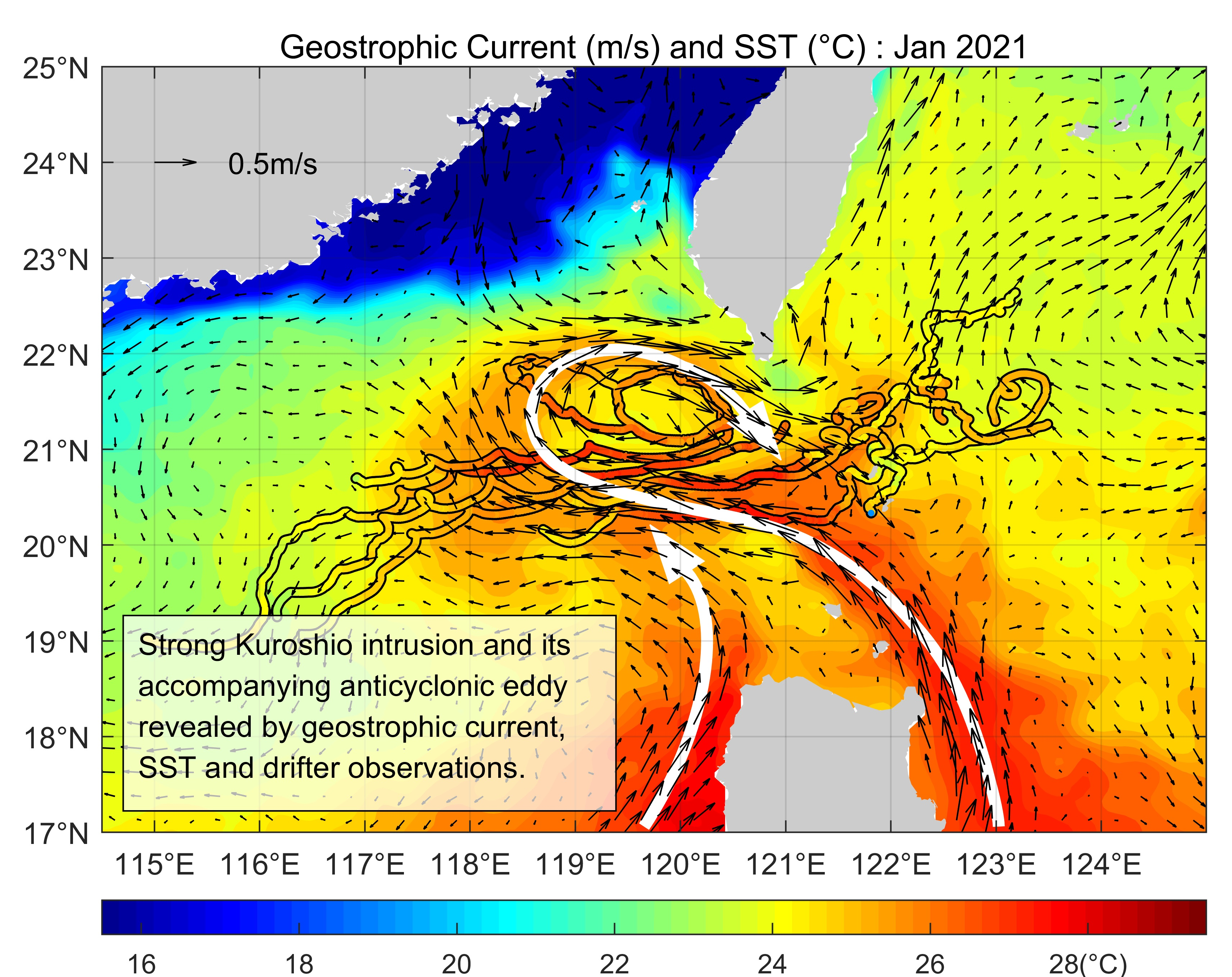
A Strong Kuroshio Intrusion into the South China Sea and Its Accompanying Cold-Core Anticyclonic Eddy in Winter 2020–2021

 , ,
, ,
Abstract
:
1. Introduction
2. Materials and Methods
3. Results
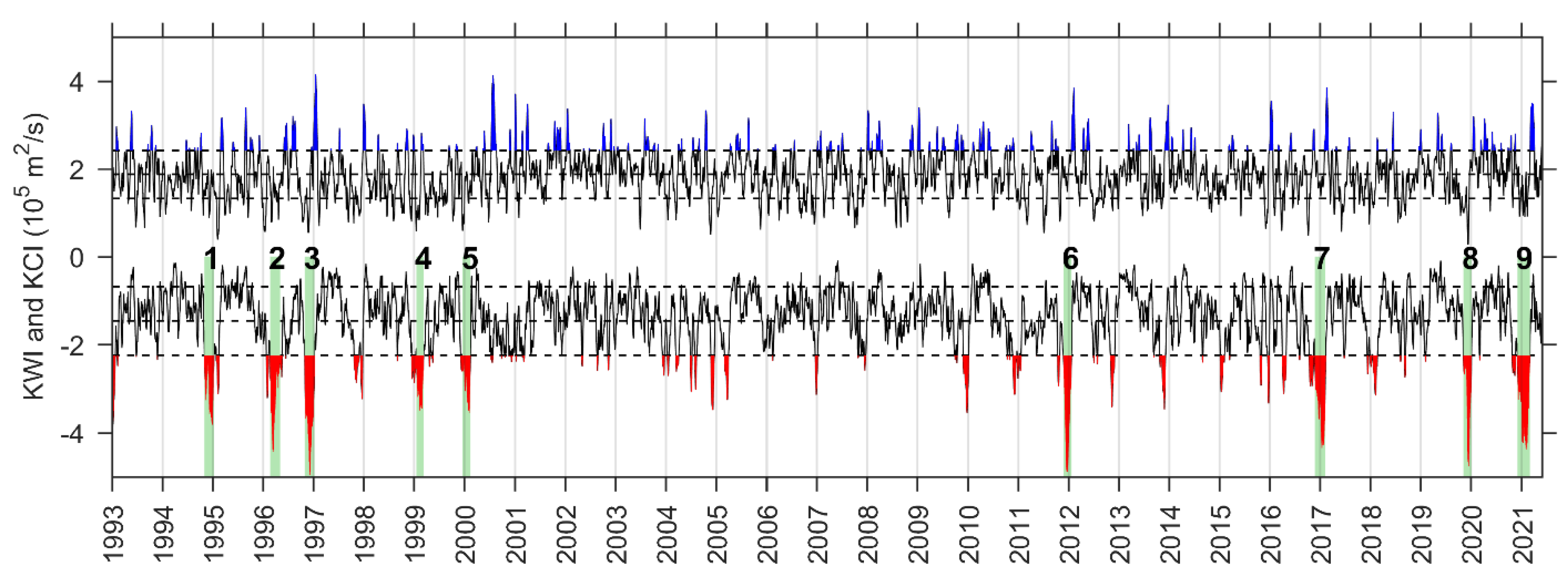
3.1. DI Performance
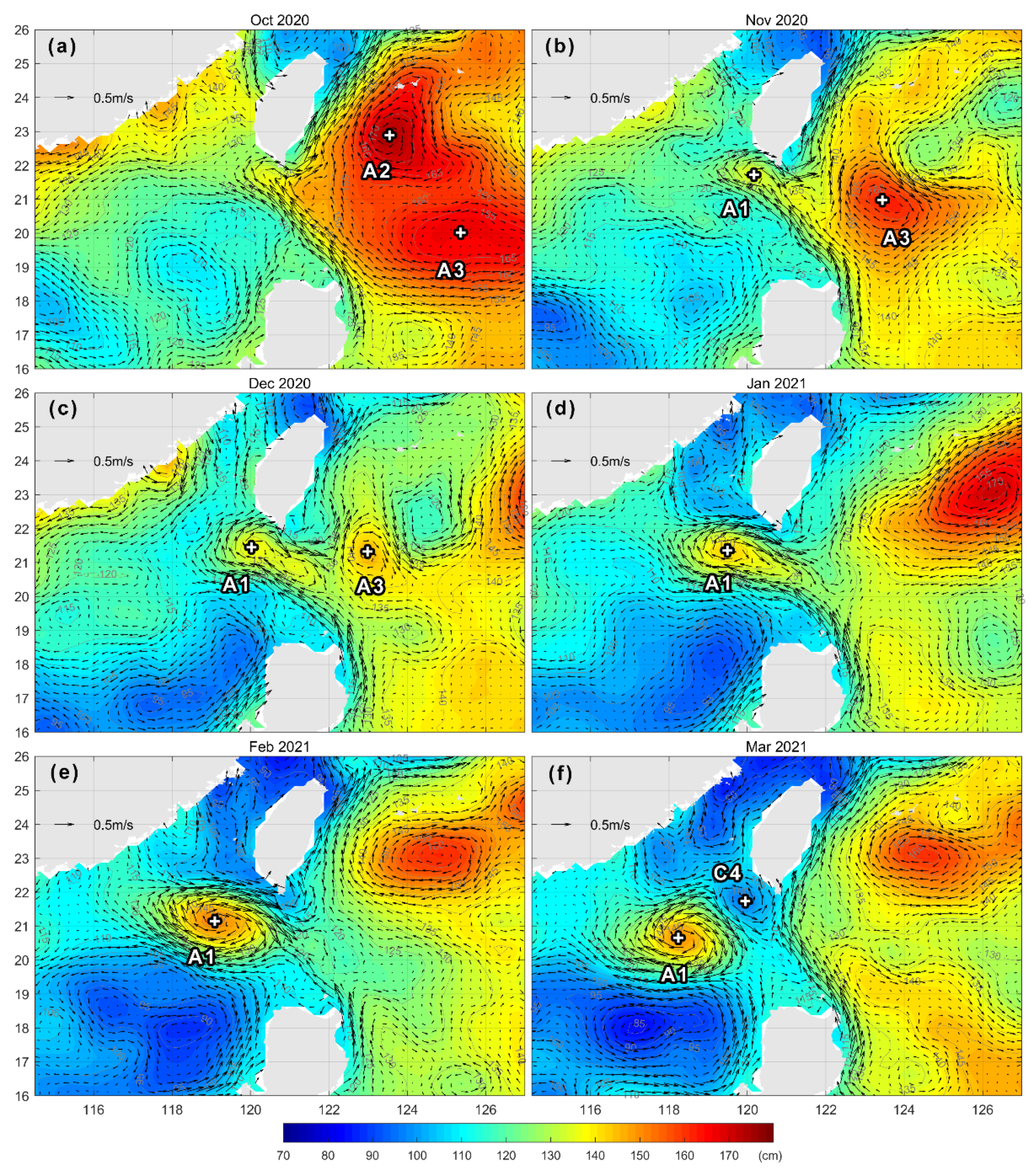
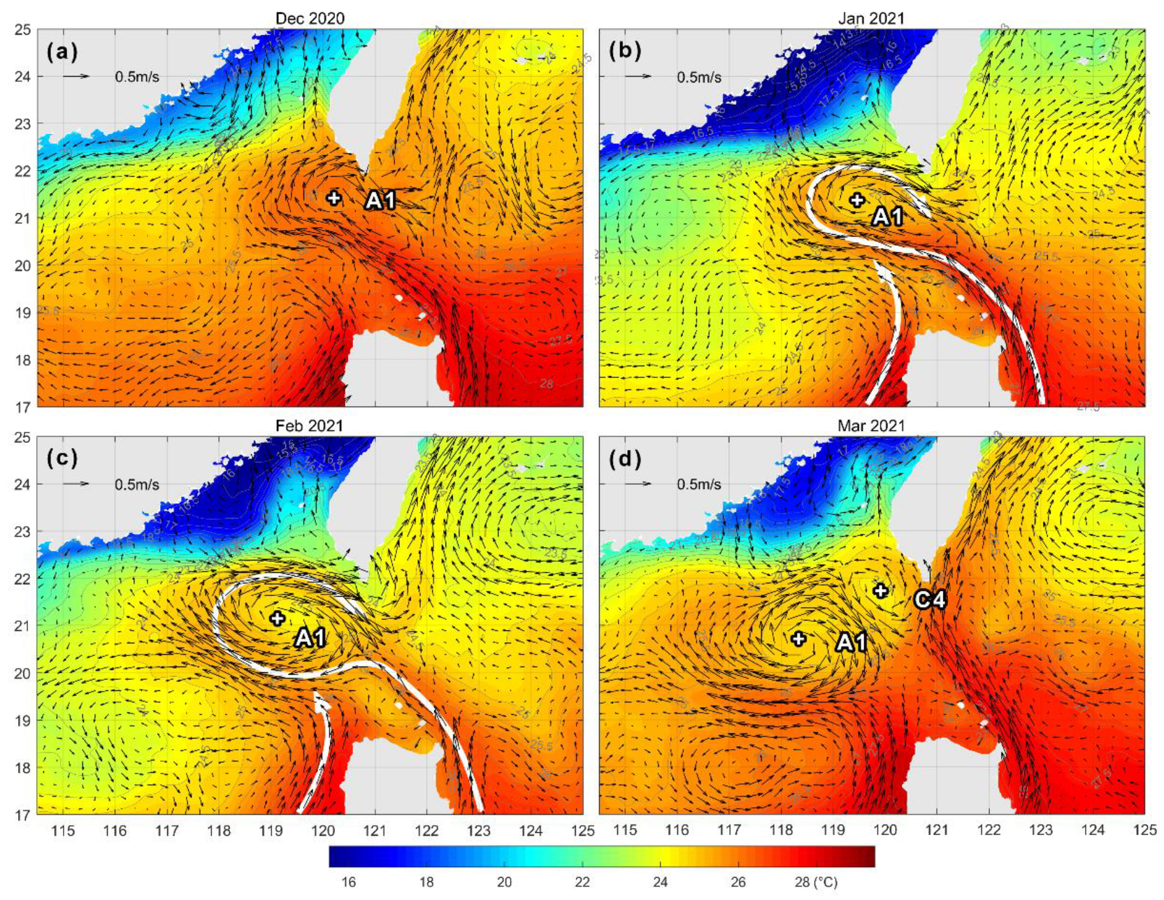
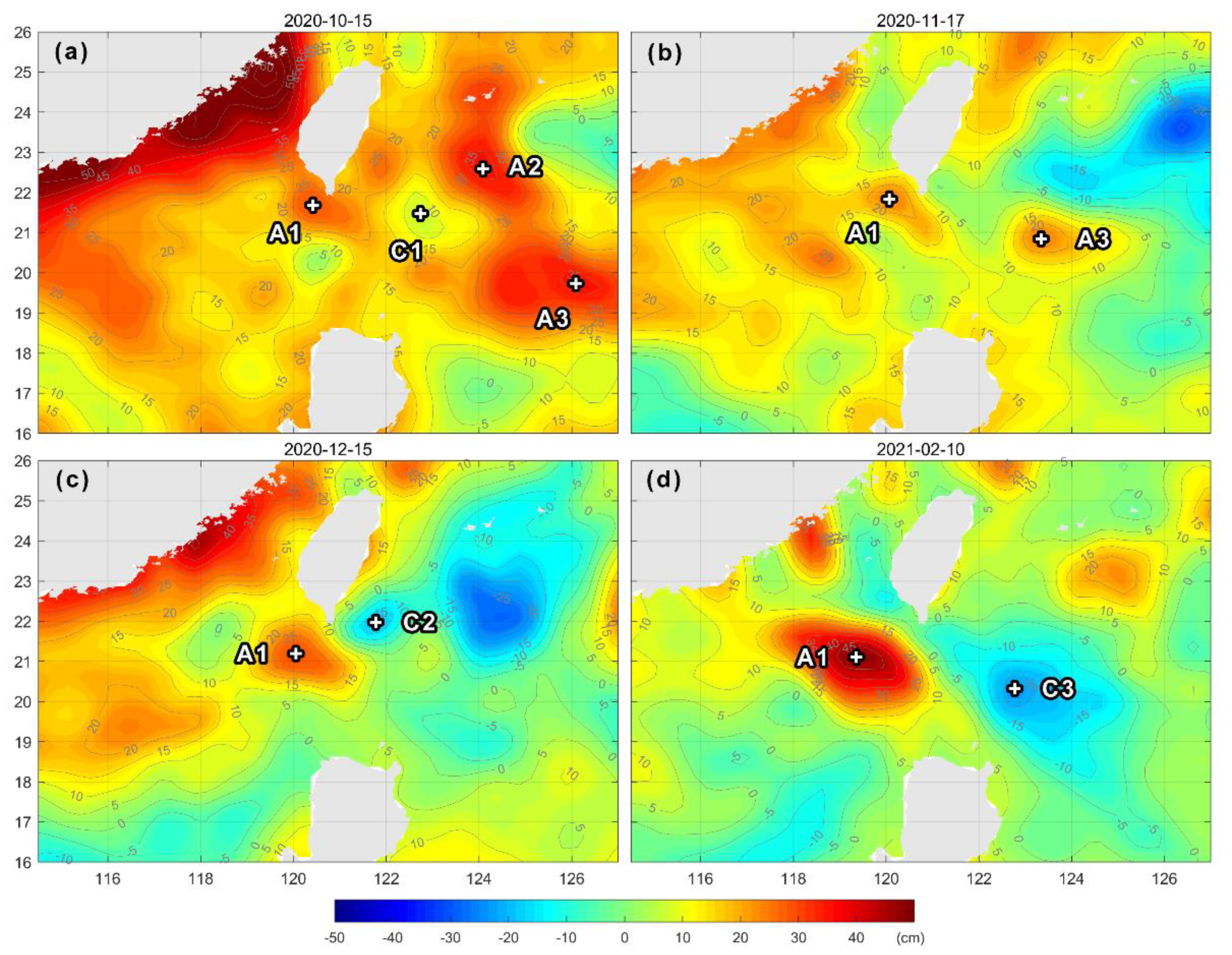
3.2. Detailed Evolution
3.3. Surface Cold-Core Structure
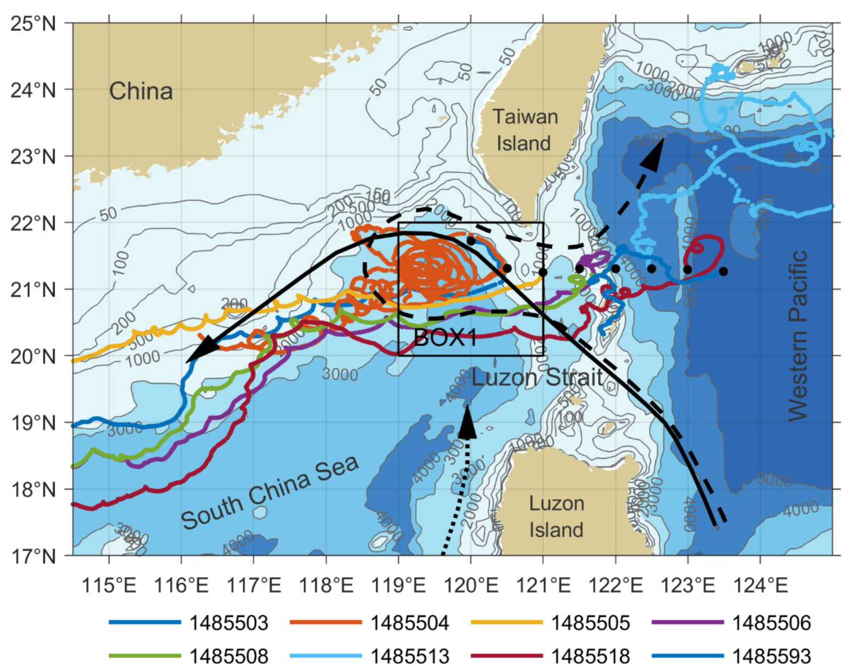
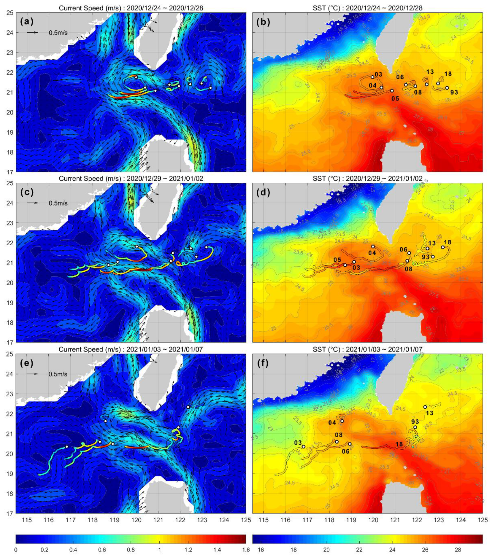
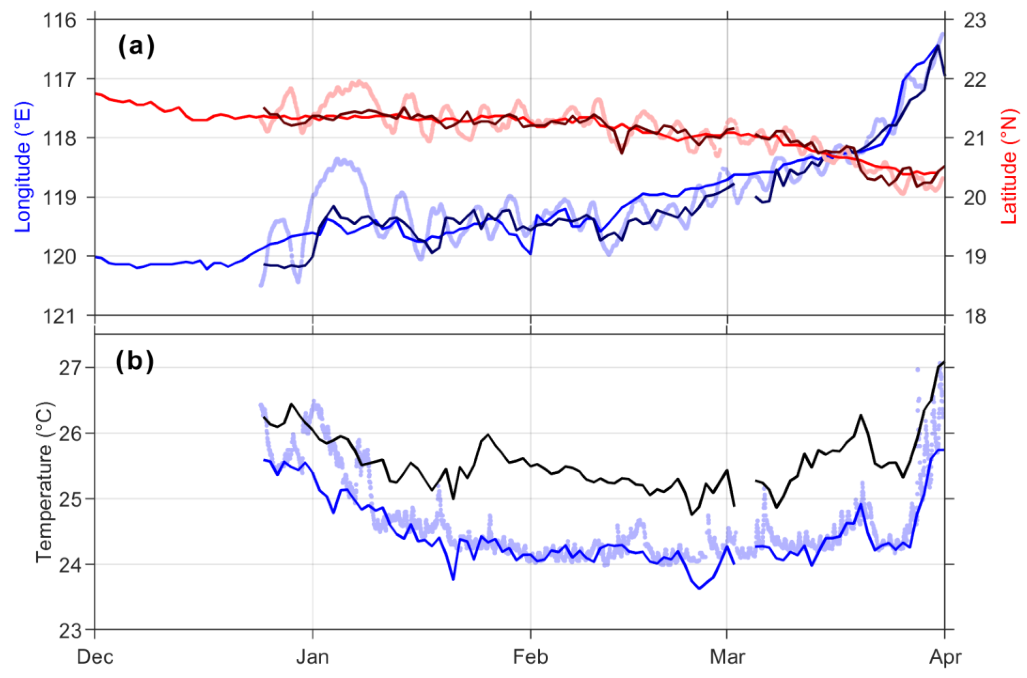
3.4. Verification by Drifters
4. Discussion
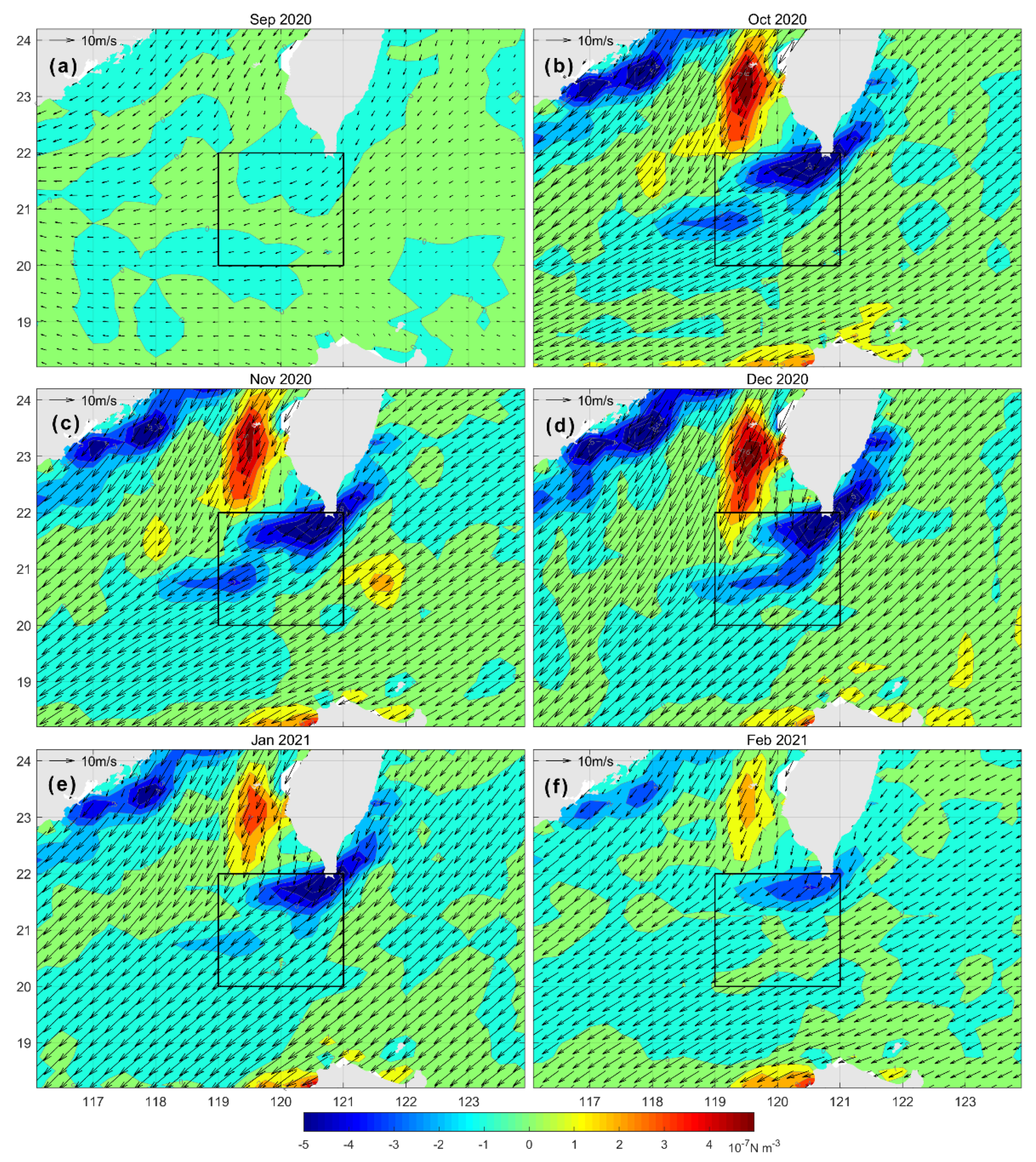
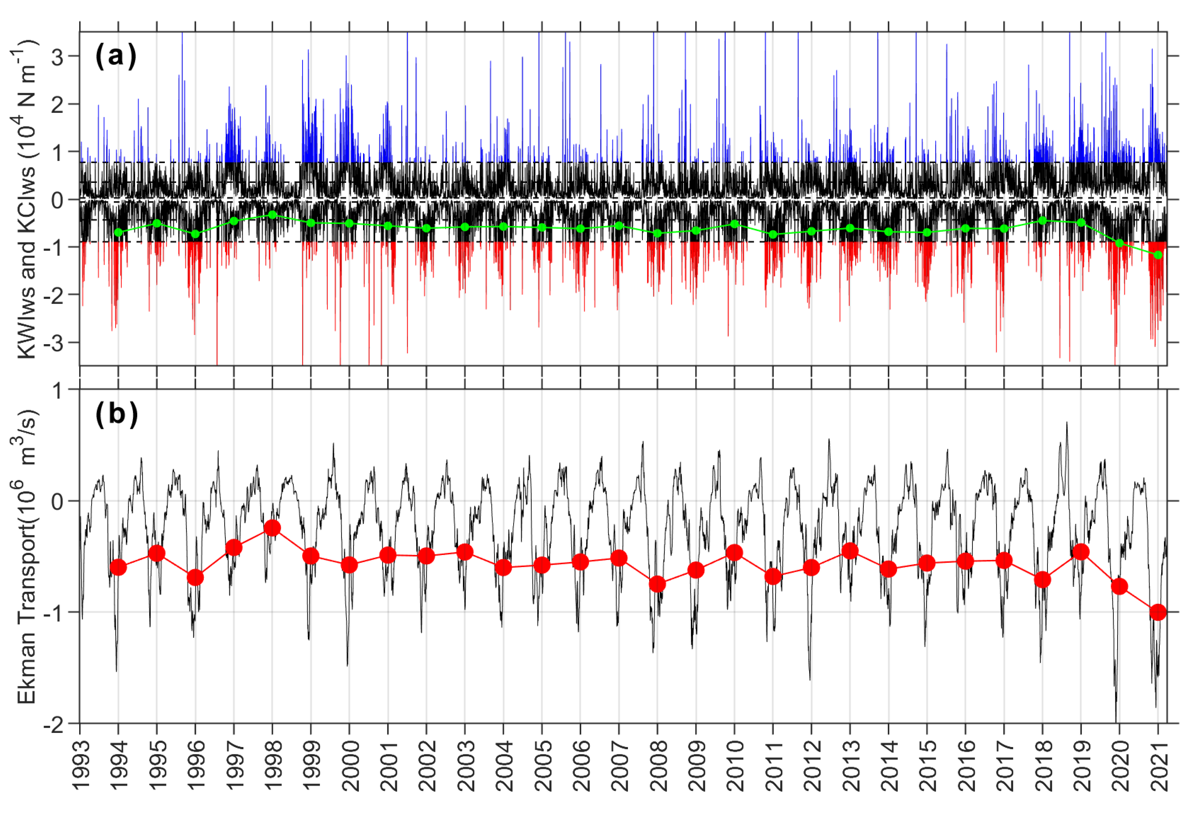
4.1. Wind Forcing
4.2. Impinging Mesoscale Eddies
4.3. Mechanism for the Surface Cold-Core Structure
5. Conclusions
Author Contributions
Funding
Data Availability Statement
Acknowledgments
Conflicts of Interest
References
- Metzger, E.J.; Hurlburt, H.E. Coupled dynamics of the South China Sea, the Sulu Sea, and the Pacific Ocean. J. Geophys. Res. Space Phys. 1996, 101, 12331–12352. [Google Scholar] [CrossRef]
- Qu, T. Upper-Layer circulation in the South China Sea. J. Phys. Oceanogr. 2000, 30, 1450–1460. [Google Scholar] [CrossRef]
- Shaw, P.-T. The seasonal variation of the intrusion of the Philippine sea water into the South China Sea. J. Geophys. Res. Space Phys. 1991, 96, 821–827. [Google Scholar] [CrossRef]
- Centurioni, L.R.; Niiler, P.P.; Lee, D.-K. Observations of Inflow of Philippine Sea Surface Water into the South China Sea through the Luzon Strait. J. Phys. Oceanogr. 2004, 34, 113–121. [Google Scholar] [CrossRef]
- Qiu, D.; Yang, T.; Guo, Z. A west-flowing current in the northern part of the South China Sea in summer. J. Trop. Oceanogr. 1984, 3, 65–73. [Google Scholar]
- Li, L.; Wu, B. A Kuroshio loop in South China Sea?—On circulations of the northeastern South China Sea. J. Oceanogr. Taiwan Strait 1989, 8, 89–95. [Google Scholar]
- Caruso, M.J.; Gawarkiewicz, G.G.; Beardsley, R.C. Interannual variability of the Kuroshio intrusion in the South China Sea. J. Oceanogr. 2006, 62, 559–575. [Google Scholar] [CrossRef]
- Nan, F.; Xue, H.; Chai, F.; Shi, L.; Shi, M.; Guo, P. Identification of different types of Kuroshio intrusion into the South China Sea. Ocean Dyn. 2011, 61, 1291–1304. [Google Scholar] [CrossRef]
- Huang, Z.; Liu, H.; Hu, J.; Lin, P. A double-index method to classify Kuroshio intrusion paths in the Luzon Strait. Adv. Atmos. Sci. 2016, 33, 715–729. [Google Scholar] [CrossRef]
- Hwang, C.; Chen, S.-A. Circulations and eddies over the South China Sea derived from TOPEX/Poseidon altimetry. J. Geophys. Res. Space Phys. 2000, 105, 23943–23965. [Google Scholar] [CrossRef]
- Wang, G.; Su, J.; Chu, P. Mesoscale eddies in the South China Sea observed with altimeter data. Geophys. Res. Lett. 2003, 30, 2121. [Google Scholar] [CrossRef] [Green Version]
- Li, L.; Nowlin, W.D.; Jilan, S. Anticyclonic rings from the Kuroshio in the South China Sea. Deep Sea Res. Part I Oceanogr. Res. Pap. 1998, 45, 1469–1482. [Google Scholar] [CrossRef]
- Wang, D.; Xu, H.; Lin, J.; Hu, J. Anticyclonic eddies in the northeastern South China Sea during winter 2003/2004. J. Oceanogr. 2008, 64, 925–935. [Google Scholar] [CrossRef]
- Guo, J.; Yuan, Y.; Xiong, X.; Guo, B. Statistics of the mesoscale eddies on both sides of the Luzon Strait. Adv. Mar. Sci. 2007, 25, 139–148. [Google Scholar]
- Jia, Y.; Chassignet, E.P. Seasonal variation of eddy shedding from the Kuroshio intrusion in the Luzon Strait. J. Oceanogr. 2011, 67, 601–611. [Google Scholar] [CrossRef]
- Nan, F.; Xue, H.; Xiu, P.; Chai, F.; Shi, M.; Guo, P. Oceanic eddy formation and propagation southwest of Taiwan. J. Geophys. Res. Space Phys. 2011, 116, 12045. [Google Scholar] [CrossRef] [Green Version]
- Wang, D.; Fang, G.; Qiu, T. The characteristics of eddies shedding from Kuroshio in the Luzon Strait. Oceanol. Limnol. Sin. 2017, 48, 673–681. [Google Scholar]
- Metzger, E.J.; Hurlburt, H.E. The Nondeterministic Nature of Kuroshio Penetration and Eddy Shedding in the South China Sea. J. Phys. Oceanogr. 2001, 31, 1712–1732. [Google Scholar] [CrossRef]
- Yuan, D.; Han, W.; Hu, D. Surface Kuroshio path in the Luzon Strait area derived from satellite remote sensing data. J. Geophys. Res. Space Phys. 2006, 111. [Google Scholar] [CrossRef] [Green Version]
- Sheremet, V.A. Hysteresis of a Western Boundary Current Leaping across a Gap. J. Phys. Oceanogr. 2001, 31, 1247–1259. [Google Scholar] [CrossRef]
- Yuan, D.; Wang, Z. Hysteresis and Dynamics of a Western Boundary Current Flowing by a Gap Forced by Impingement of Mesoscale Eddies. J. Phys. Oceanogr. 2011, 41, 878–888. [Google Scholar] [CrossRef]
- Gan, J.; Qu, T. Coastal jet separation and associated flow variability in the southwest South China Sea. Deep Sea Res. Part I Oceanogr. Res. Pap. 2008, 55, 1–19. [Google Scholar] [CrossRef]
- Xiu, P.; Chai, F.; Shi, L.; Xue, H.; Chao, Y. A census of eddy activities in the South China Sea during 1993–2007. J. Geophys. Res. Space Phys. 2010, 115, 03012. [Google Scholar] [CrossRef] [Green Version]
- Wang, G.; Chen, D.; Su, J. Winter Eddy Genesis in the Eastern South China Sea due to Orographic Wind Jets. J. Phys. Oceanogr. 2008, 38, 726–732. [Google Scholar] [CrossRef]
- Wu, C.-R.; Hsin, Y.-C. The forcing mechanism leading to the Kuroshio intrusion into the South China Sea. J. Geophys. Res. Space Phys. 2012, 117. [Google Scholar] [CrossRef] [Green Version]
- Jie, Z.; De-Hai, L. Response of the Kuroshio Current to Eddies in the Luzon Strait. Atmos. Ocean. Sci. Lett. 2010, 3, 160–164. [Google Scholar] [CrossRef]
- Lien, R.-C.; Ma, B.; Cheng, Y.-H.; Ho, C.-R.; Qiu, B.; Lee, C.M.; Chang, M.-H. Modulation of Kuroshio transport by mesoscale eddies at the Luzon Strait entrance. J. Geophys. Res. Oceans 2014, 119, 2129–2142. [Google Scholar] [CrossRef]
- Zhong, L.; Hua, L.; Luo, D. The Eddy–Mean Flow Interaction and the Intrusion of Western Boundary Current into the South China Sea–Type Basin in an Idealized Model. J. Phys. Oceanogr. 2016, 46, 2493–2527. [Google Scholar] [CrossRef]
- Hu, J.; Zheng, Q.; Sun, Z.; Tai, C.-K. Penetration of nonlinear Rossby eddies into South China Sea evidenced by cruise data. J. Geophys. Res. Space Phys. 2012, 117. [Google Scholar] [CrossRef]
- Zheng, Q.; Tai, C.-K.; Hu, J.; Lin, H.; Zhang, R.-H.; Su, F.-C.; Yang, X. Satellite altimeter observations of nonlinear Rossby eddy–Kuroshio interaction at the Luzon Strait. J. Oceanogr. 2011, 67, 365–376. [Google Scholar] [CrossRef]
- Chang, Y.-L.; Miyazawa, Y.; Guo, X. Effects of the STCC eddies on the Kuroshio based on the 20-year JCOPE2 reanalysis results. Prog. Oceanogr. 2015, 135, 64–76. [Google Scholar] [CrossRef]
- Nan, F.; Xue, H.; Chai, F.; Wang, D.; Yu, F.; Shi, M.; Guo, P.; Xiu, P. Weakening of the Kuroshio Intrusion into the South China Sea over the Past Two Decades. J. Clim. 2013, 26, 8097–8110. [Google Scholar] [CrossRef] [Green Version]
- Yang, Q.; Liu, H.; Lin, P. The effect of oceanic mesoscale eddies on the looping path of the Kuroshio intrusion in the Luzon Strait. Sci. Rep. 2020, 10, 636. [Google Scholar] [CrossRef]
- Yasuda, I.; Ito, S.-I.; Shimizu, Y.; Ichikawa, K.; Ueda, K.-I.; Honma, T.; Uchiyama, M.; Watanabe, K.; Sunou, N.; Tanaka, K.; et al. Cold-Core Anticyclonic Eddies South of the Bussol’ Strait in the Northwestern Subarctic Pacific. J. Phys. Oceanogr. 2000, 30, 1137–1157. [Google Scholar] [CrossRef]
- Ji, J.; Dong, C.; Zhang, B.; Liu, Y. An oceanic eddy statistical comparison using multiple observational data in the Kuroshio Extension region. Acta Oceanol. Sin. 2017, 36, 1–7. [Google Scholar] [CrossRef]
- Sun, W.; Dong, C.; Tan, W.; He, Y. Statistical Characteristics of Cyclonic Warm-Core Eddies and Anticyclonic Cold-Core Eddies in the North Pacific Based on Remote Sensing Data. Remote Sens. 2019, 11, 208. [Google Scholar] [CrossRef] [Green Version]
- McGillicuddy, D. Formation of Intrathermocline Lenses by Eddy–Wind Interaction. J. Phys. Oceanogr. 2015, 45, 606–612. [Google Scholar] [CrossRef] [Green Version]
- Good, S.; Fiedler, E.; Mao, C.; Martin, M.J.; Maycock, A.; Reid, R.; Roberts-Jones, J.; Searle, T.; Waters, J.; While, J.; et al. The Current Configuration of the OSTIA System for Operational Production of Foundation Sea Surface Temperature and Ice Concentration Analyses. Remote Sens. 2020, 12, 720. [Google Scholar] [CrossRef] [Green Version]
- Lumpkin, R.; Özgökmen, T.; Centurioni, L. Advances in the Application of Surface Drifters. Annu. Rev. Mar. Sci. 2017, 9, 59–81. [Google Scholar] [CrossRef] [Green Version]
- Elipot, S.; Lumpkin, R.; Perez, R.C.; Lilly, J.M.; Early, J.J.; Sykulski, A. A global surface drifter data set at hourly resolution. J. Geophys. Res. Oceans 2016, 121, 2937–2966. [Google Scholar] [CrossRef]
- Chaigneau, A.; Eldin, G.; Dewitte, B. Eddy activity in the four major upwelling systems from satellite altimetry (1992–2007). Prog. Oceanogr. 2009, 83, 117–123. [Google Scholar] [CrossRef]
- Chelton, D.B.; Schlax, M.G.; Samelson, R.M. Global observations of nonlinear mesoscale eddies. Prog. Oceanogr. 2011, 91, 167–216. [Google Scholar] [CrossRef]
- Hu, J.; Kawamura, H.; Hong, H.; Qi, Y. A Review on the Currents in the South China Sea: Seasonal Circulation, South China Sea Warm Current and Kuroshio Intrusion. J. Oceanogr. 2000, 56, 607–624. [Google Scholar] [CrossRef]
- Zu, T.; Gan, J.; Erofeeva, S.Y. Numerical study of the tide and tidal dynamics in the South China Sea. Deep Sea Res. Part I Oceanogr. Res. Pap. 2008, 55, 137–154. [Google Scholar] [CrossRef]
- Farris, A.; Wimbush, M. Wind-induced Kuroshio intrusion into the South China Sea. J. Oceanogr. 1996, 52, 771–784. [Google Scholar] [CrossRef]
- Zhang, Z.; Zhao, W.; Qiu, B.; Tian, J. Anticyclonic Eddy Sheddings from Kuroshio Loop and the Accompanying Cyclonic Eddy in the Northeastern South China Sea. J. Phys. Oceanogr. 2017, 47, 1243–1259. [Google Scholar] [CrossRef] [Green Version]


| Drifter No. | Deployment Date | Deployment Longitude | Deployment Latitude | End Date 1 |
|---|---|---|---|---|
| 1485503 | 24 December 2020 | 120.0°E | 21.8°N | 30 January 2021 |
| 1485504 | 24 December 2020 | 120.5°E | 21.3°N | 31 March 2021 |
| 1485505 | 26 December 2020 | 121.0°E | 21.3°N | 15 February 2021 |
| 1485506 | 26 December 2020 | 121.5°E | 21.3°N | 30 January 2021 |
| 1485508 | 26 December 2020 | 122.0°E | 21.3°N | 30 January 2021 |
| 1485513 | 26 December 2020 | 122.5°E | 21.3°N | 31 March 2021 |
| 1485518 | 26 December 2020 | 123.0°E | 21.3°N | 30 January 2021 |
| 1485593 | 26 December 2020 | 123.5°E | 21.3°N | 8 January 2021 |
| Event No. | Start Date | End Date | Period (day) | Minimum KWI 1 | Integral KWI 2 |
|---|---|---|---|---|---|
| 1 | 2 November 1994 | 10 January 1995 | 69 | −3.82 | −212.6 |
| 2 | 22 February 1996 | 4 May 1996 | 72 | −4.43 | −230.8 |
| 3 | 30 October 1996 | 8 January 1997 | 70 | −4.96 | −269.2 |
| 4 | 18 January 1999 | 12 March 1999 | 53 | −3.49 | −164.3 |
| 5 | 20 December 1999 | 14 February 2000 | 56 | −3.55 | −165.1 |
| 6 | 27 November 2011 | 24 January 2012 | 58 | −4.89 | −217.8 |
| 7 | 24 November 2016 | 10 February 2017 | 78 | −4.35 | −274.5 |
| 8 | 8 November 2019 | 5 January 2020 | 58 | −4.76 | −190.7 |
| 9 | 4 December 2020 | 4 March 2021 | 90 | −4.38 | −316.0 |
| Wang et al. [11] | Guo et al. [14] | Jia et al. [15] | Nan et al. [16] | Wang et al. [17] | Present Study | |
|---|---|---|---|---|---|---|
| Diameter 1 | A: 244 | A: 225 | A: 160 | A: 128 | A: 166 | 381 |
| - | M: 300 | M: 200 | M: 162 | M: 320 | ||
| Amplitude 2 | A: 12 | - | - | A: 12 | A: 11 | 50 |
| M: 32 | - | - | M: 20 | M: 47 | ||
| Distance 3 | A: 195 | - | - | A: 433 | A: 218 | >820 |
| - | - | - | M: 1879 | M: 1020 | ||
| Lifespan 4 | A: 108 | - | - | A: 75 | A: 29 | >182 |
| - | M: 57 | - | M: 273 | M: 135 | ||
| Speed 5 | A: 2.1 | A: 4.5 | A: 10.0 | A: 6.4 | A: 8.3 | 5.2 |
| - | M: 9.0 | M: 16.0 | M: 11.0 | M: 35.0 |
Publisher’s Note: MDPI stays neutral with regard to jurisdictional claims in published maps and institutional affiliations. |
© 2021 by the authors. Licensee MDPI, Basel, Switzerland. This article is an open access article distributed under the terms and conditions of the Creative Commons Attribution (CC BY) license (https://creativecommons.org/licenses/by/4.0/).
Share and Cite
Sun, Z.; Hu, J.; Chen, Z.; Zhu, J.; Yang, L.; Chen, X.; Wu, X. A Strong Kuroshio Intrusion into the South China Sea and Its Accompanying Cold-Core Anticyclonic Eddy in Winter 2020–2021. Remote Sens. 2021, 13, 2645. https://doi.org/10.3390/rs13142645
Sun Z, Hu J, Chen Z, Zhu J, Yang L, Chen X, Wu X. A Strong Kuroshio Intrusion into the South China Sea and Its Accompanying Cold-Core Anticyclonic Eddy in Winter 2020–2021. Remote Sensing. 2021; 13(14):2645. https://doi.org/10.3390/rs13142645
Chicago/Turabian StyleSun, Zhenyu, Jianyu Hu, Zhaozhang Chen, Jia Zhu, Longqi Yang, Xirong Chen, and Xuewen Wu. 2021. "A Strong Kuroshio Intrusion into the South China Sea and Its Accompanying Cold-Core Anticyclonic Eddy in Winter 2020–2021" Remote Sensing 13, no. 14: 2645. https://doi.org/10.3390/rs13142645