8-Day and Daily Maximum and Minimum Air Temperature Estimation via Machine Learning Method on a Climate Zone to Global Scale

Abstract

Air temperature (Ta) is a required input in a wide range of applications, e.g., agriculture. Land Surface Temperature (LST) products from Moderate Resolution Imaging Spectroradiometer (MODIS) are widely used to estimate Ta. Previous studies of these products in Ta estimation, however, were generally applied in small areas and with a small number of meteorological stations. This study designed both temporal and spatial experiments to estimate 8-day and daily maximum and minimum Ta (Tmax and Tmin) on three spatial scales: climate zone, continental and global scales from 2009 to 2018, using the Random Forest (RF) method based on MODIS LST products and other auxiliary data. Factors contributing to the relation between LST and Ta were determined based on physical models and equations. Temporal and spatial experiments were defined by the rules of dividing the training and validation datasets for the RF method, in which the stations selected in the training dataset were all included or not in the validation dataset. The RF model was first trained and validated on each spatial scale, respectively. On a global scale, model accuracy with a determination coefficient (R²) > 0.96 and root mean square error (RMSE) < 1.96 °C and R² > 0.95 and RMSE < 2.55 °C was achieved for 8-day and daily Ta estimations, respectively, in both temporal and spatial experiments. Then the model was trained and cross-validated on each spatial scale. The results showed that the data size and station distribution of the study area were the main factors influencing the model performance at different spatial scales. Finally, the spatial patterns of the model performance and variable importance were analyzed. Both daytime and nighttime LST had a significant contribution in the 8-day Tmax estimation on all the three spatial scales; while their contribution in daily Tmax estimation varied over different continents or climate zones. This study was expected to improve our understanding of Ta estimation in terms of accuracy variations and influencing variables on different spatial and temporal scales. The future work mainly includes identifying underlying mechanisms of estimation errors and the uncertainty sources of Ta estimation from a local to a global scale.

1. Introduction

Air temperature (Ta) plays an important role in energy balance and many near-surface processes such as plant photosynthesis, land surface phenology [1] and evapotranspiration [2], etc. In addition, this essential climate variable is desired in various agrometeorological models and applications [3]. At present, Ta is typically measured at meteorological stations 2 m above the ground. Ground measurements from meteorological stations provide accurate, discrete Ta information for specific locations [4]. However, it is challenging to get spatially continuous Ta data from the discrete and non-uniform meteorological measurements due to the complexity of the land surface conditions and patterns [5], especially in the areas with sparse stations, such as the African plateau region [6,7].

Satellite remote sensing observations from global imaging sensors show great potential to characterize spatially continuous patterns of Ta on a global scale [8]. The science-grade quality of the Land Surface Temperature (LST) data collected by MODIS has proven valuable for monitoring land surface dynamics over large areas [3,9,10]. The Ta generally has a strong relationship to LST, as the atmosphere is mainly heated from the ground up through longwave infrared radiation [4,11,12]. However, the land surface energy balance is a complex phenomenon that varies with space and depends on many factors [13]. The commonly used methods to estimate Ta from satellite-based LST products can be divided into three distinct types of approaches:

• The first type is the index-base method such as Temperature-Vegetation Index (TVX) first proposed by Nemani and running [14], which assumes that dense vegetation canopy temperature approximates Ta [15,16]. This method is easily applied with no auxiliary data. It is widely used in the estimation of regional near-surface Ta [5,16,17]. However, the TVX method is based on dense vegetation canopy temperature and the negative relationship between the Normalized Difference Vegetation Index (NDVI) and LST. Accordingly, its application is limited and conditional. For example, Vancutsem et al. [17] showed that the TVX method did not adapt to different ecosystems over Africa due to the non-significant relationship between Ts and NDVI in their study.
• The second category is the physically-based method based on surface energy balance. For example, Sun et al. [18] and Zhu et al. [19] proposed surface energy balance theory-based methodologies to build a quantitative relationship between LST and Ta. However physically-based models are complex and these methods require large amounts of information that are usually unavailable from remote sensing observations (e.g., wind speed) [12,20]. The complexity and difficulty for application limited its extensive applications in previous studies.
• The final class of methods estimates Ta from the local statistical relationship between Ta and other variables, e.g., LST, NDVI, retrieved by remote sensing. Statistical methods are the most commonly used methods [21,22,23], including regression method [21], hierarchical Bayesian model [24], and machine learning (ML) methods, such as random forest (RF) method, support vector machine (SVM) method, deep belief network (DBN) method, and neural networks (NN) method [10,25,26,27,28,29]. In general, these statistical methods perform well within the spatial and time frame in which they were developed, but the accuracy might decrease when extended in time and space [16].

There are still three pending issues that need to be further studied relating to Ta estimation based on satellite-derived LST. Firstly, many efforts have been made to use these above-mentioned methods to estimate Ta in different local regions, e.g., European countries [12], USA [30], Asian areas [7], Africa [17], Antarctica [25], etc. Previous studies generally applied to small areas or a small number of meteorological stations. At a local scale, many previous studies reported different relationships between Ta and LST and reached divergent or even contradictory conclusions in studies, e.g., if the land cover plays an important role in Ta estimation or not [12,31,32,33,34] and if nighttime LST can outperform in daily maximum Ta than daytime LST estimation or not [12,31,32,33,34]. For example, usually, daytime and nighttime LST is expected to be more effective and simply used in estimating daily maximum and minimum Ta (hereafter Tmax and Tmin), respectively [12,31,32,33,34], as the observation time of daytime and nighttime LST from MODIS is close to the occurrence of the maximum and minimum LST and Ta, respectively. However, Zhang et al. [35] and Zeng et al. [4] showed that using nighttime LST resulted in higher accuracy Tmax estimations than using daytime LST. Then, many studies tried to use daytime as well as nighttime LST to estimate Tmax, and some of these studies reported a significant improvement in estimation accuracy [36,37,38,39], while some did not find a significant improvement [40]. Phan et al. [40] showed that whether the Tmax is more correlated with nighttime LST than daytime LST can differ between stations. Therefore, what factors influence the performance of daytime and nighttime LST requires further study and analysis on larger and different spatial scales. Secondly, the earth’s surface is heated by solar radiation, while the atmosphere is mainly heated from the ground up through longwave infrared radiation [4]. LST and Ta interaction is controlled by the complex energy balance and affected by many ever-changing factors (e.g., cloud cover, surface roughness, wind speed and soil moisture) [4,41]. In addition, air masses usually strike the local energy balance and some of these variables are not available from remote sensing data. In previous studies, usually, a limited number of factors were taken into consideration, as a result, the models were generally applicable within the spatial and time frame in which they were developed, but the accuracy might decrease when extended in time and space [4,40]. Thirdly, Ta estimation models based on remote sensing data aim to map spatially continuous Ta at the pixel level. However, the ground observations are unavailable for most of the pixels. Accordingly, Ta estimation models need to be built based on the stations or pixels with ground observations and applied to the pixels without ground measurement points, i.e., a model that is able to successfully predict beyond the locations of the training stations is expected. However, many previous studies validated models using data from the stations that were also included in the calibration datasets. For example, Phan et al. [4,21,40], Benali et al. [12] and Zeng et al. [4] randomly divided the datasets into calibration and validation datasets, regardless of the temporal and spatial components by mixing all the observations into a global dataset, i.e., regardless of measurement date or location (station) [12]. The stations from calibration were usually included in the training dataset as well. Furthermore, some studies, such as Zhu et al. [5], Janatian et al. [5] and Didari and Zand-Parsa [36] used the data from certain year/years to calibrate the model and used the data from other year/years to validate, i.e., the stations from calibration and validation datasets were totally overlayed. These models optimized for the included stations/pixels generally have good performance, but how about the applications extended to additional stations/pixels that are not endowed with measurement points?

In order to fill the research gap in the above-mentioned three issues, this study aims to: (1) investigate the relationship between LST and Ta from a climate zone scale to a global scale, e.g., what factors contribute to Ta estimations based on the observations from satellite imagery and the spatial variation of errors at different spatial scales, considering that different results were derived in previous studies when applied in different local areas; (2) explore the variables that are available on a regional scale and that can affect the relationship between LST and Ta to estimate Ta based on physical equations and models and (3) validate and compare Ta estimation based on both a temporal and spatial basis by designing both temporal and spatial experiments in which the stations used to validate the model are all included or not in the training datasets, respectively, considering that Ta estimation models are usually calibrated by the discrete ground observations, while spatially continuous Ta needs to be inferred from discrete observations. While many previous studies only validate the Ta estimation models on a temporal basis. This study aims to use the RF method as a mean to study the 8-day and daily Ta estimation based on remotely sensed data from a climate zone to a global scale as the Ta estimation at these two temporal scales, i.e., 8-day and daily scale are the most desirable in relevant applications and the most widely studied in the previous studies. It is expected to provide valuable information for further application and study of Ta estimation based on remotely sensed data at different areas and temporal or spatial scales.

2. Materials and Method

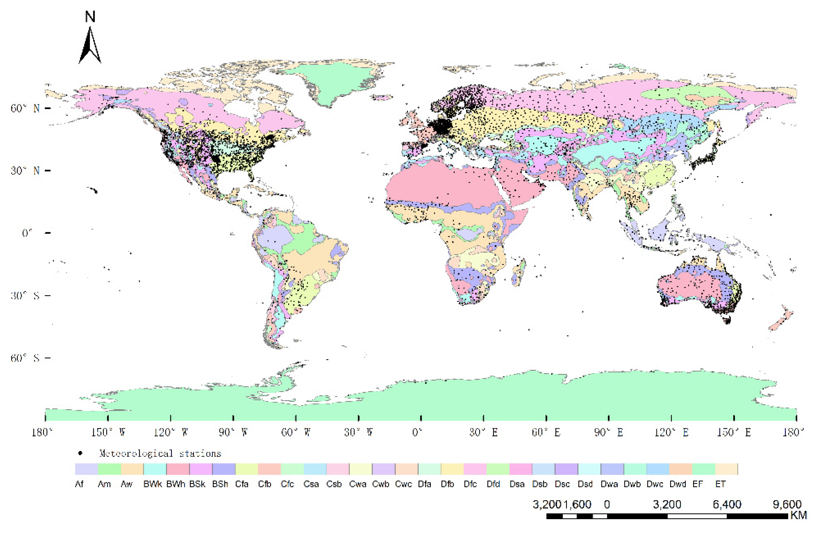
2.1. Study Area

The study areas include the global continent except for the polar areas where few ground observations have been collected, including 6 continents: Asia, North America, Europe, Africa, South America, Oceania (Figure 1). Ta estimation model based on the RF method was applied and studied on three spatial scales, i.e., climate zone, continental, global scale. The Köppen-Geiger system was used to divide the climate zones on the earth. It classifies climate into five main classes and 30 sub-types (see [42]). The five main classes include tropical zone (A), arid zone (B), temperate zone (C), cold zone (D) and polar zone (E). Each main class is divided into two to four secondary classes. The abbreviation of each climate zone begins with the representative letter of the five classes, followed by the abbreviation of the secondary classes and tertiary classes, respectively. For example, the climate zone BWh which begins with B and consists of three letters: “B”, “W” and “h” is hot, arid desert climate. It is the tertiary subclass of the arid zone. The classes with little ground observations available (Csc, Cfc, Cwc, Dsd, EF) from NOAA were not included in this study.

2.2. Data Collection and Processing

2.2.1. Meteorological Observation Data

Daily Tmax and Tmin measured in meteorological stations from 2009 to 2018 were downloaded from the GHCN (Global Historical Climatology Network)-Daily database from NOAA’s National Climatic Data Center [43]. This database is a composite of climate records from numerous data sources from land surface stations across the globe that were merged and checked for quality assurance [4]. GHCN-Daily provides daily maximum and minimum air temperature, i.e., daily Tmax and Tmin. The 8-day Tmax and Tmin were calculated by averaging the daily Tmax and Tmin during the corresponding 8-day window, respectively. GHCN-Daily is denser over North America and Eurasia than over South America, Antarctica and Africa. The stations for Tmax and Tmin estimations were selected when continuous Tmax or Tmin observations were available in at least 8 years during the period from 2009 to 2018. In addition, only one station was randomly selected when there was more than one station in the same 0.05° × 0.05° pixel. There were a total of 5650 stations and, after filtering, 5443 were selected and used for the study of Tmax and Tmin estimation in this study.

2.2.2. Satellite-Derived Observation Data

Satellite-derived data/products used in this study includes daily and 8-day composite global 0.05° LST from Aqua (MYD11C1 and MYD11C2), daily global 0.05° surface reflectance from Terra (MOD09CMG), 16-day vegetation indices from Terra (MOD13C1), yearly global 0.05° land cover type from Terra and Aqua (MCD12C1), daily Bidirectional Reflectance Distribution Function (BRDF) and Albedo dataset (MCD43C3), daily and 8-day composite snow cover 0.05° product from Aqua (MYD10C1 and MYD10C2), daily and 8-day composite 0.05° downward surface shortwave radiation of Global Land Surface Satellite (GLASS) products, net radiation products (CERES_NETFLUX) from NASA Langley Research Center. LST products from Aqua were used as some studies (e.g., [12]) reported higher estimation accuracy using LST observations from Aqua than Terra, due to the fact that the MODIS Aqua overpass time is closer to the time of both Tmax and Tmin than Terra’s. While similar to most of the related research (e.g., [5,10]), surface reflectance and vegetation indices from Terra were used to calculate and present the vegetation variations of the study areas. The daily NDVI was calculated from the surface reflectance products by the equation of $\mathrm{NDVI}=({\rho }_{\mathrm{nir}}-{\rho }_{\mathrm{r}})/({\rho }_{\mathrm{nir}}+{\rho }_{\mathrm{r}})$, where ${\rho }_{\mathrm{r}}$ and ${\rho }_{\mathrm{nir}}$ refer to the visible red and near-infrared band of MODIS.

2.2.3. Auxiliary Data

Additional auxiliary data used to refine the analysis included: Shuttle Radar Topography Mission (SRTM) global elevation data at 3-arc second (~90 m resolution) [44], Köppen-Geiger climate classification map [42], and the distance from the sea coast. The distance from the sea coast was calculated using the Haversine formulation (Equations (1) and (2)):

$$\mathrm{Haversine}(d/R)=haversin({\phi }_2-{\phi }_1)+\cos ({\phi }_1)\cos ({\phi }_2)haversin(\Delta \lambda )$$

(1)

$$haversin(\theta )={\sin }^2(\theta /2)=(1-\cos (\theta ))/2$$

(2)

where R is the Earth radius, φ₁, φ₂ are the latitude of the two pixels, ∆λ is the difference value of longitude of the two pixels.

2.2.4. Data Processing

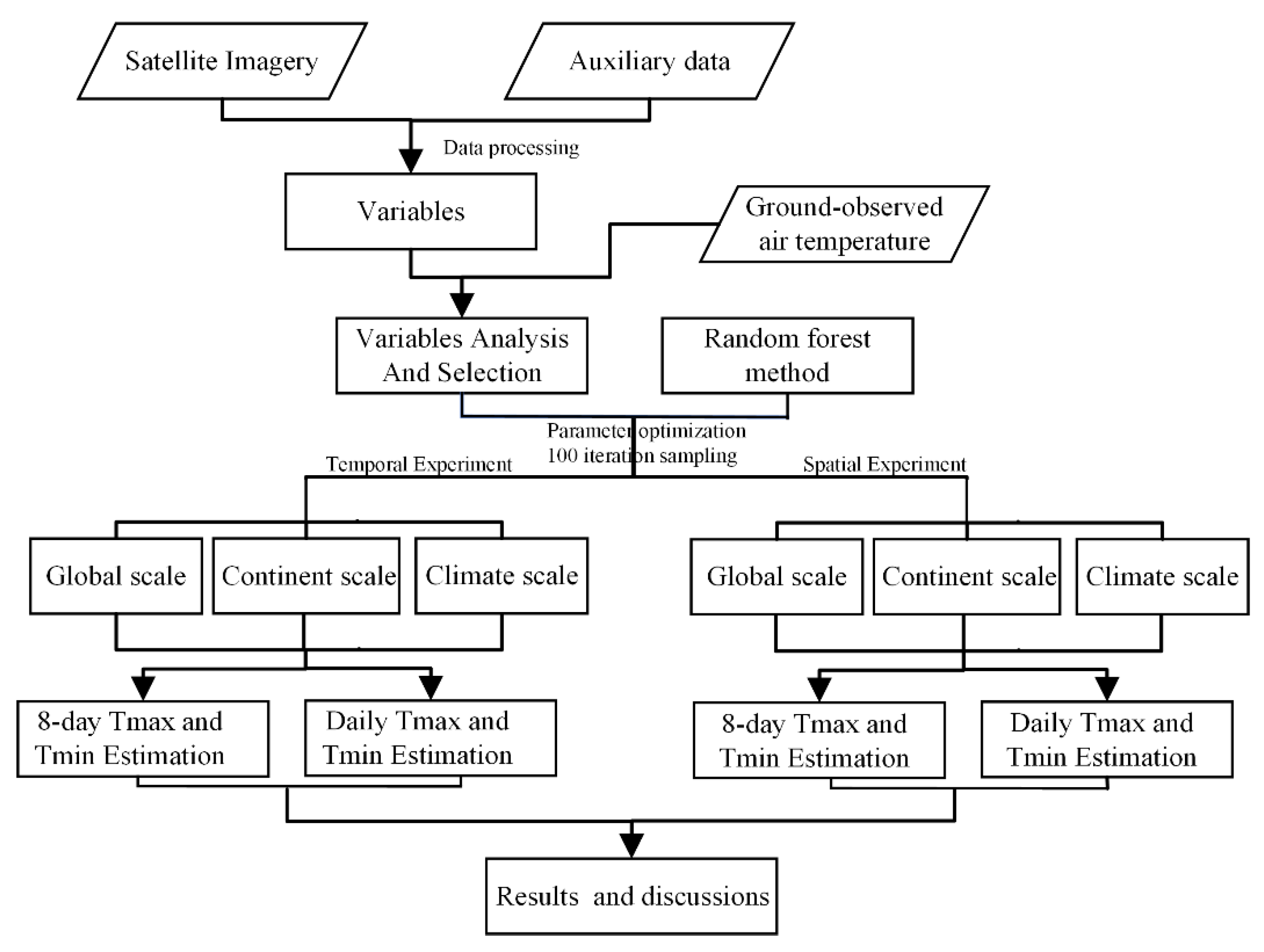
Low-quality ground and satellite-derived observations were eliminated based on the quality flag data. Remote sensing-based LST and surface reflectance data are usually significantly influenced by errors caused by cloud cover, aerosol and large sensor viewing angles, etc. Thus, only the pixels that were flagged in the MODIS quality assurance data as cloud-free and of high quality were retained.

Data from multiple sources have different spatial and temporal resolutions. All the input data were integrated into the same time scale for the daily and 8-day average Ta estimation. All the variables were resampled to 0.05° × 0.05° resolution to estimate the 0.05° × 0.05° Ta. The resolution 0.05° × 0.05° was selected based on the research and results of previous studies. Yan et al. [45] showed that Ta retrieval at 0.05° did not affect the calibration and validation of Ta. Some existing research even suggested a spatially averaged LST series over a window of 5 × 5 km to 25 × 25 km original MODIS LST pixels instead of a single MODIS pixel (250 m~1000 m) [19,46,47]. As the interaction between the land surface and the near-surface atmosphere is not limited to individual pixels alone but also operates in the regional scale [19,46,47], i.e., Ta observed at the station is not only affected by the LST of the single MODIS pixel where the station locates but also the nearby pixels within a window.

Table 1. The acronym and description of the variables used in this study.

Abbreviation	Data Description	Data Source	Estimation
LSTday	Daytime LST	MODIS LST products	8-day and daily Tmax and Tmin
LSTnight	Nighttime LST	MODIS LST products	8-day and daily Tmax and Tmin
LSTday1	Daytime LST observed on 1 day before estimation	MODIS LST products	daily Tmax and Tmin
LSTday2	Daytime LST observed on 2 days before estimation	MODIS LST products	daily Tmax and Tmin
LSTday3	Daytime LST observed on 3 days before estimation	MODIS LST products	daily Tmax and Tmin
LSTnight1	Nighttime LST observed on 1 day before estimation	MODIS LST products	daily Tmax and Tmin
LSTnight2	Nighttime LST observed on 2 days before estimation	MODIS LST products	daily Tmax and Tmin
LSTnight3	Nighttime LST observed on 3 days before estimation	MODIS LST products	daily Tmax and Tmin
Elevation	Elevation	SRTM global elevation data	8-day and daily Tmax and Tmin
NR	Net radiation	NASA Langley Research Center	8-day and daily Tmax and Tmin
DSR	Downward Shortwave Radiation	GLASS Downward Shortwave Radiation product	8-day and daily Tmax and Tmin
SC	Snow cover	MODIS snow cover product	8-day and daily Tmax and Tmin
OLD	Distance from the ocean	Calculated from Haversine formulation	8-day and daily Tmax and Tmin
LU	Land-use type	MODIS Land cover product	8-day and daily Tmax and Tmin
Season	Day of year for daily estimation; Sequence number of 8-day within the year (1–46)		8-day and daily Tmax and Tmin
NDVI	Normalized difference vegetation index	MODIS surface reflectance product for daily estimation and vegetation indices products for 8-day estimation	8-day and daily Tmax and Tmin
Climate	Climate zone	Köppen-Geiger climate classification	8-day and daily Tmax and Tmin
WSA_vis	White-sky Albedo in Visible albedo	GLASS Albedo Product	8-day and daily Tmax and Tmin
BSA_vis	Black-sky albedo in Near-Infrared band	GLASS Albedo Product	8-day and daily Tmax and Tmin
WSA_shortwave	White-sky albedo in shortwave band	GLASS Albedo Product	8-day and daily Tmax and Tmin
BSA_shortwave	Black-sky albedo in shortwave band	GLASS Albedo Product	8-day and daily Tmax and Tmin
WSA_nir	White-sky albedo in Near-Infrared band	GLASS Albedo Product	8-day and daily Tmax and Tmin
BSA_nir	Black-sky albedo in Visible band	GLASS Albedo Product	8-day and daily Tmax and Tmin
Day_view_ time	Local solar time of daytime LST observation	MODIS LST products	8-day and daily Tmax and Tmin
Night_view_ time	Local solar time of nighttime LST observation	MODIS LST products	8-day and daily Tmax and Tmin

shows the variables used in 8-day and daily Ta estimation. Daily Ta estimation used six LST variables observed on the days before estimation, i.e., LSTday1, LSTday2, LSTday3, LSTnight1, LSTnight2 and LSTnight3 as daily Ta estimations are significantly influenced by air advection, undergoing dramatic changes. For example, air masses usually strike the local energy balance, and the day-to-day difference of Ta can reflect the changes of air masses, as well as the sources of air masses and their major paths [4]. The daily estimations including the six LST variables have significantly improved accuracy (with ~0.5 °C lower RMSE, not shown) than the estimations without including the six variables.

2.3. Method

2.3.1. Variable Selection Based on Physical Relationship between Ta and LST

Solar radiation is the main source of the earth’s energy. When solar radiation reaches the earth’s surface, part of the energy is reflected and part of the energy is absorbed by the surface. This energy exchange process can be expressed by the surface energy balance (SEB) [4]. Net radiation is the sum of soil heat flux, sensible heat flux, and latent heat flux (Equation (3)) and it is calculated from the incoming and outgoing all wave radiation fluxes (Equations (4) and (5)) [48]. The sensible heat flux is often physically parametrized as Equation (4) by using the bulk transfer of heat fluxes between the land surface and atmosphere [49].

$$R_n=G+H+LE$$

(3)

$$R_n=R_s\downarrow -R_s\uparrow +R_L\downarrow -R_L\uparrow$$

(4)

$$R_n=(1-{\rho }_0)R_s\downarrow +{\epsilon }_a{\epsilon }_s\sigma {T_s}^4-{\epsilon }_s\sigma {T_a}^4$$

(5)

$$H=\frac{r{C}_p}{r_a}(T_{aero}-T_a)$$

(6)

where $R_n$ is net radiation, G is soil heat flux, H is sensible heat flux, and LE is latent heat flux. $R_s\downarrow$ is the downwelling shortwave radiation, $R_s\uparrow$ is the upwelling shortwave radiation. $R_L\downarrow$ is the downwelling longwave radiation and $R_L\uparrow$ is the upwelling longwave radiation. ${\epsilon }_a$ is the volumetric heat capacity of air, $r_a$ is the air aerodynamic resistance, The Greek letters $\rho$ and σ represent albedo and the Stefan–Boltzmann constant, ${\epsilon }_a$ and ${\epsilon }_s$ represent atmospheric and land surface emissivity, $T_s$ is land surface temperature and $T_{aero}$ is aerodynamic temperature which is usually substituted by LST in applications [49,50].

Many investigations have shown that mid-day soil heat flux/net radiation fraction is reasonably predictable from the empirical relationship of vegetation (Equations (7) and (8)) [51].

$$G=\Gamma R_n$$

(7)

$$\Gamma =\frac{T_s-273.15}{r_0}(0.32r_0+0.62{r_0}^2)(1-0.987{NDVI}^2)$$

(8)

where $\Gamma$ is the soil heat/net radiation flux density ratio and $r_0$ refers to broadband surface albedo.

By combining (Equations (3)–(8)), the variables building the relationship between Ts and Ta relate to net radiation, albedo, downwelling shortwave radiation, NDVI, etc. These variables can be estimated from remote sensing data. Furthermore, considering the diurnal cycle of LST [52] and Ta gradient with topographic elevation [53], the relationship between Tmax and the instantaneous observation LST also depends on elevation and the view time when LST is observed [10]. Due to the difference in thermal capacity of water and land, the Ta and LST interaction is also affected by the energy exchange between the ocean and nearby ground as well as the air above the areas [54]. Therefore, other factors, such as the Julian day, data view time, elevation, distance from the sea coast, were also taken into consideration. [12,29,53,54,55].

2.3.2. Ta Estimation Based on the RF Method

In this study, we applied the RF method to build Tmax and Tmin estimation models from a regional to a global scale. As RF has proven to be promising, flexible, and easily applied in areas with heterogeneous landscapes and it was highly recommended in estimating land surface parameters, e.g., Ta, soil moisture, etc. with satellite observations and available auxiliary data [12,25,28].

As shown in Figure 2, in order to investigate the estimation accuracy of the RF method on both a “temporal” and “spatial” basis, two independent experiments: a temporal and spatial experiment, were designed and conducted to estimate both 8-day and daily Tmax and Tmin in this study. In both experiments, the refined dataset was divided into two groups: training and validation datasets with a 70/30% split into these groups using a simple random sampling. As for each iteration, the RF model was trained on the training dataset and then used to estimate Tmax and Tmin based on the variables in the validation dataset. Random sampling was used to run 100 iterations for each estimation of 8-day and daily Tmax and Tmin. The averaged accuracy over the validation dataset in the 100 iterations was presented for each estimation in the results and discussions section.

As for the random sampling in the temporal experiment, the data including all the stations observed from 70% of the study period from 2009 to 2018 was randomly selected as the training dataset and the remaining 30% of data was used as the validation dataset, i.e., the training datasets were randomly selected based on the rule that the stations to be estimated in the validate dataset are all the same as those in the training dataset, but the observation time is different. While in the spatial experiment, the data observed at 70% of the stations in the study period from 2009 to 2018 were randomly selected as the training dataset and the data from the remaining 30% of the stations were used as the validation dataset, i.e., the stations to be estimated in the test dataset are all not included in the training dataset.

RF is an ensemble machine learning technique developed to improve the classification and regression tree (CART) methods that combine tree predictors. Two parameters must be optimized in RF: the number of regression trees (ntree) and the number of input variables per node (mtry). Considering the large data volume and the time cost, the number of regression trees (ntree) is set as 100 and the number of input variables per node (mtry) was tested from 1/3 to all the total number of variables by one iteration of random sampling for each kind of estimation (e.g., daily Tmax). To find the optimal mtry values, ntree were optimized based on the root mean square error (RMSE) of the calibration using the training dataset [56].

2.3.3. Model Evaluation and Validation

The statistical relationship between the estimated Ta and the observed Ta from the ground was analyzed in this study. Two main statistical performance measures were used including the coefficient of determination (R²) and root-mean-square error (RMSE, Equation (9)).

$$\mathrm{RMSE}={\left\{\left({\displaystyle \sum _1^n{\left(y_{est}-y_{obs}\right)}^2}/n\right)\right\}}^{1/2}$$

(9)

where $y_{est}$ is estimated Ta from MODIS LST and other auxiliary variables, and $y_{obs}$ is the corresponding observed Ta from the meteorological station.

3. Results and Discussion

3.1. Model Performance When Trained and Validated on Global, Continental and Climate Zone Scales

The RF model was calibrated and validated on global, continental and climate zone scales, respectively. The results were shown in

Table 2. Estimation accuracy of 8-day and daily Tmax and Tmin in both spatial and temporal experiments on a global scale.

	8-Day Tmax		8-Day Tmin		Daily Tmax		Daily Tmin
	R2	RMSE	R2	RMSE	R2	RMSE	R2	RMSE
S	0.96	1.84	0.94	1.96	0.95	2.55	0.95	2.55
T	0.97	1.65	0.96	1.75	0.96	2.31	0.96	2.31

Note: S represents the spatial estimation, T represents the temporal estimation hereafter.

, Figure 3 and Figure 4. A higher estimation accuracy was observed in the temporal experiment than in the spatial experiment for both 8-day and daily Tmax and Tmin estimation on all three scales. As in the temporal experiment, the RF method was optimized for the stations included in the training dataset as well as the validation dataset. While in the spatial experiment, the RF model as a supervised learning model trained by the data of stations included in the training dataset might not favor the application to the other stations in the validation datasets.

In addition, generally higher accuracy was observed in 8-day Ta estimation than that in daily estimation, which was in accordance with other studies (e.g., [56]) as daily Ta and LST affected by the ever-changing factors show higher variability than the 8-day composites [17], which are more difficult to be accurately captured. This is because the surface Ta is determined by two physical processes, the heating effect produced by the longwave radiation from the land surface and the advective effect resulting from turbulent flow exchange. The advection, e.g., air mass, usually strikes the local energy balance, then becomes one of the reasons for energy imbalance and contributes to the uncertainty of energy influxes. There is a time lag for the establishment of a new balance between Ta and LST [4]. The R_n on the left side of Equation (3) is not equal to items (𝐻 + 𝐿𝐸 + 𝐺) on the right side of Equation (1) at the local basis before the establishment of new balance.

Specifically, on a global scale, high accuracy of 8-day Tmax and Tmin estimation in both spatial and temporal experiments was achieved (R² > 0.94 and RMSE < 2 °C). Daily Ta estimation obtained comparable accuracy with 8-day estimation in terms of R², while a clearly higher RMSE (2.31~2.55 °C) was observed for daily Ta estimation in both spatial and temporal experiments than that in 8-day Ta estimation.

For 8-day Tmax and Tmin estimation on a continental scale, the RF method generally achieved high accuracy in the temporal experiments for all the six areas with R² > 0.9 and RMSE < 2 °C, while relatively lower but still acceptable results were obtained with RMSE ~2 °C in spatial experiments. As for daily Tmax and Tmin estimation on a continental scale, the RF method generally yielded an inferior performance with R² > 0.8 and RMSE < 2.8 °C. The highest estimation accuracy was observed in Oceania for both Tmax and Tmin estimation (Figure 3). On a climate zone scale, model accuracy with R² > 0.9 and RMSE < 3 °C and R² > 0.85 and RMSE < 3.5 °C was achieved for 8-day and daily Ta estimation, respectively, in most of the climate zones (Figure 4).

Both 8-day and daily Tmax and Tmin estimation accuracy varied spatially over different continents or climate zones (Figure 3 and Figure 4). As the relationship between Ta and LST is strongly affected by heterogeneity in the environmental factors and land surface characteristics that control the energy balance of the land–atmosphere system [57,58]. Ta estimation accuracy in terms of both R² and RMSE was related to the total data size used in the RF models as well as regional disparity. For example, significantly lower accuracy of 8-day Ta estimation was achieved in the spatial experiments for Africa and South America (Figure 3). The reason for this might be the sparse distribution and consequently the under-representation of the meteorological stations in these two areas (Figure 1). In addition, a smaller difference between the estimation accuracy in temporal and spatial experiments was observed in the climate zones with larger data sizes, e.g., Dfa, Dfb, Dfc, Cfa, Cfb.

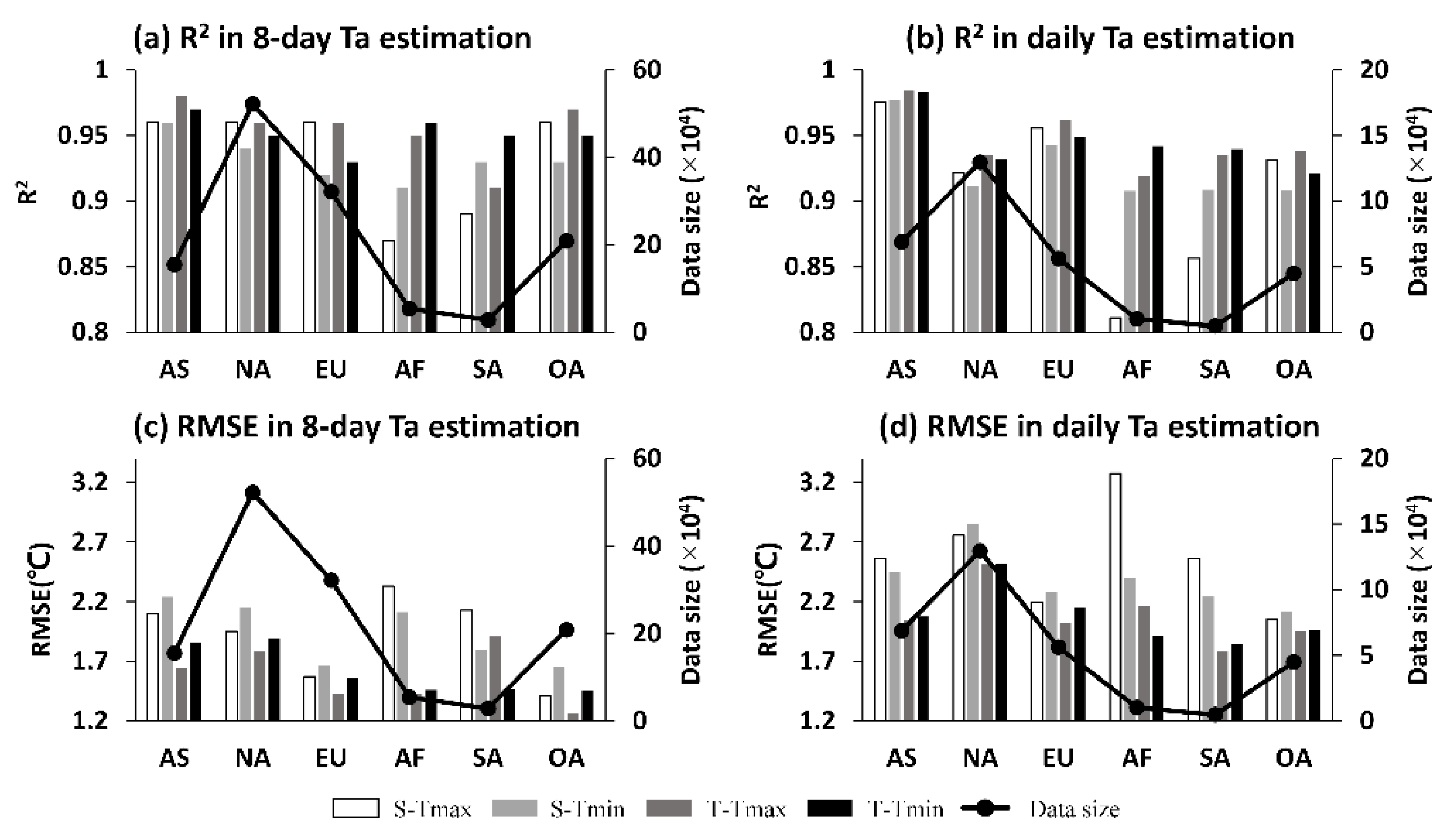
3.2. Model Performance When Trained and Cross-Validated on Global, Continental and Climate Zone Scales

Figure 5 shows the averaged 8-day and daily Tmax and Tmin estimation accuracy of involved stations in spatial experiments when using the model trained and cross-validated at different scales. For example, Figure 5c shows the 8-day Tmax and Tmin estimation accuracy at each climate zone when using the models trained on a global and climate zone scale, respectively.

As shown in Figure 5a,b, both 8-day and daily Ta estimation accuracies using the model trained on a continental scale (hereafter continental model) were higher than those using the model trained on a global scale (hereafter global model) in terms of RMSE in each continent except daily Tmin estimation in South America. In addition, the corresponding accuracy differences between the global and continental models tend to be more significant in the continents with sparse observation stations, e.g., Africa, and not obvious in the continents with more observation stations, e.g., North America because on the global scale, the training data from the NOAA dataset is strongly biased towards America and Europe in terms of the station density, data quantity and even data quality and not favored to Africa and South America. Therefore, the global model tended to be biased in Africa and SA, whose accuracy was lower than that of the continental models with even small size of the training dataset. It indicates that the global model is not favorable to Ta estimation on a continents scale considering the data size (>120 stations in each continent) as well as the complex and divergent landscapes in different continents.

It is shown from Figure 5c,d that both 8-day and daily Ta estimation accuracies of climate zone models were lower than those using the global model in terms of RMSE in most of the climate zones. Similarly, the corresponding accuracy differences between the global and climate zone models tended to be more significant in the climate zones with fewer observation stations, e.g., Cfc, Dwd, Dfd, and not obvious in the climate zones with more observation stations, e.g., Cfa, Dfa, Dfb, Dfc, because at the climate zone scale, the sizes of the dataset in most of the climate zones are too small (<60 stations), which can bring about inferior performance in the model.

Overall, the uneven distribution of the observation stations can introduce biases in the areas with fewer observation data. A very small data size can also bring about the low accuracy of the model. Accordingly, in the areas with sparse observation stations (<60), the dataset observed in other areas, especially the areas with similar climate and landscape to the study areas can be helpful for Ta estimation using the RF method.

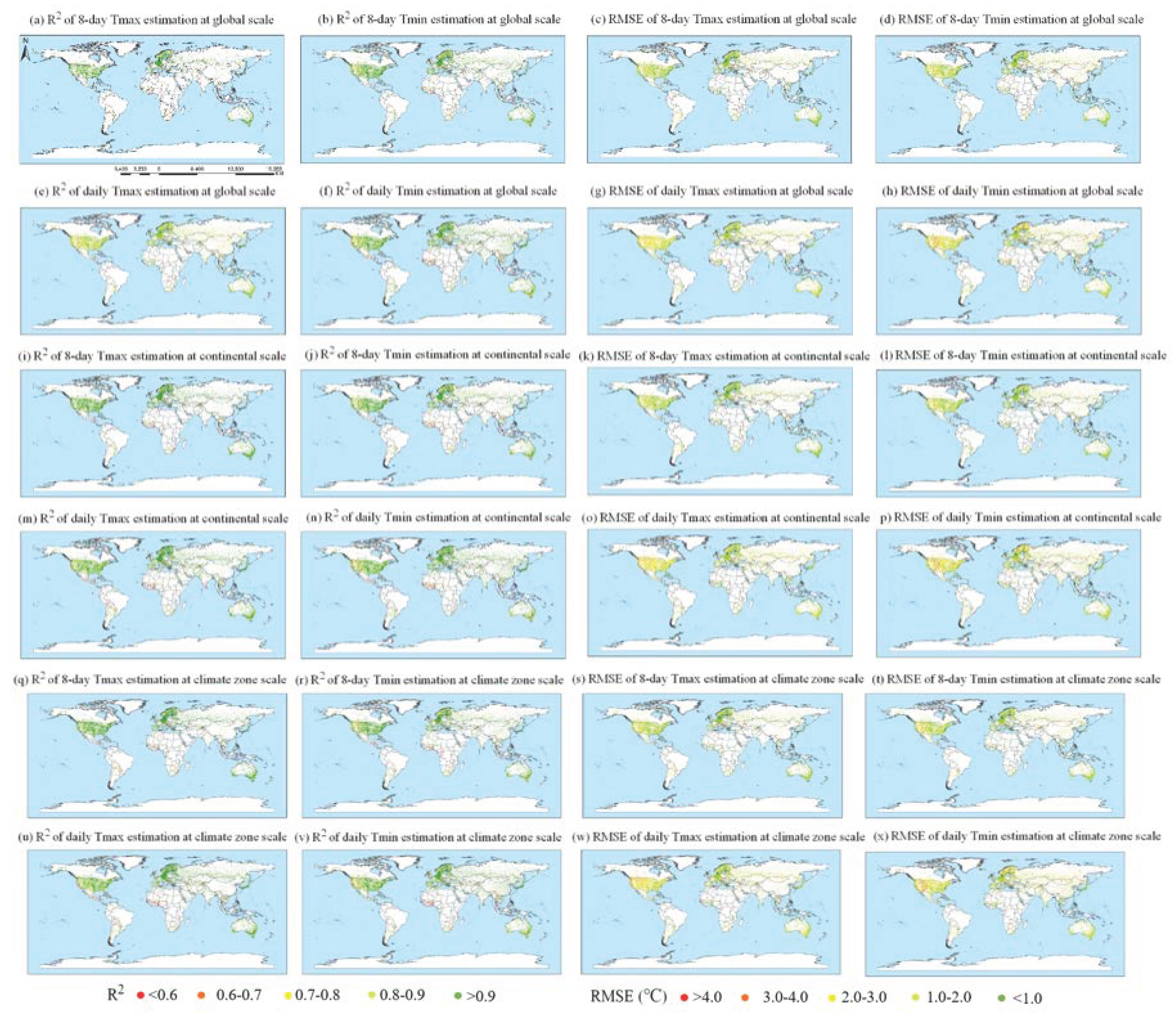
3.3. Spatial Patterns of Model Performance

Figure 6 shows the spatial patterns of the 8-day and daily Tmax and Tmin estimation model performance in spatial experiments. The RF method delivered a stronger performance in 8-day Ta estimation than that in daily Ta estimation at most of the stations. As shown in the spatial patterns, the spatial pattern, as well as the estimation accuracy at the three different scales are all similar, which also indicates that the variables included in this study can generally cover the different conditions all over the world.

The spatial patterns of 8-day Ta estimation accuracy are similar to that of daily Ta estimation. The spatial patterns of the accuracy of Tmax estimation are also similar to that of Tmin estimation. For example, the accuracy of both 8-day and daily Ta estimations were relatively higher in European areas and the eastern United States, while a corresponding lower estimation accuracy was observed in Africa and the western United States in terms of both R² and RMSE because the factors influencing Tmax and Tmin estimation were similar at a certain location and the spatial patterns of the size of training datasets were also similar for the four Ta estimation models, i.e., 8-day and daily Tmax and Tmin estimation.

First, the accuracy depends on the complexity of land surface characteristics as well as those of the station surroundings [46,47,59]. For example, obviously, inferior Ta estimation accuracy was observed in the areas with higher elevation and heterogeneous surface, e.g., the western United States, the east coast of Australia, Norway as complexity and heterogeneity of land surface, for one thing, can dampen the accuracy of the remote-sensed retrievals themselves, especially LST by increasing the uncertainty of emissivity and therefore influencing the accuracy of Ta estimation [12]. Errors in LST retrieval are usually larger in highly heterogeneous areas [12,29]. For another, the Topography effect can further complicate the Tmax-LST relationship. Mutiibwa et al. [60] showed that the increasing terrain roughness diminished the relation between Ta and LST.

Second, under-parameterization is another problem in remote sensing-based Ta estimation, especially for the above-mentioned heterogeneous areas, as the observations derived from the sensors cannot account for all the major variables affecting the complicated interactions between the land surface and the near-surface atmosphere [16,17]. For example, Ta is influenced by the air advection from the local radiation budget as well as the surrounding areas [47,61]. Sohrabinia et al. [47,61] reported a closer relationship between LST and Ta under a slight instability in the local atmosphere, as this can strengthen the local turbulent heat fluxes as compared to a stable atmosphere with no wind that might restrict the heat exchange between LST and Ta [62]. In a windy atmosphere, air advection from the adjacent areas (e.g., ocean or mountains) accounts more for the Ta variation than the local sensible heat fluxes [63]. However, certain influencing factors, e.g., wind speed and wind direction, are difficult to be retrieved from remote sensing data.

Third, the data size is also an important factor that can significantly affect the model performance, especially for the data-driven models, e.g., machine learning models. The areas with sparse observation stations always have inferior performance in the global model or the smaller scale model, e.g., Africa and South America because the global model is always biased towards the areas with more stations that contribute more in the training of the global model. On a climate scale, small sizes of training datasets can also affect the model performance.

Furthermore, the areas near the equator had low estimation accuracy in terms of R², though most of the areas near the equator except Africa had acceptable estimation accuracy in terms of RMSE. The reason for low R² might be the small variation of Tmax or Tmin all through the year in the areas near the equator due to the high solar radiation, as compared to the many other areas with larger Ta variation (higher temperatures in summer and lower temperatures in winter). The small Ta variation can result in a lower R² value under a similar RMSE.

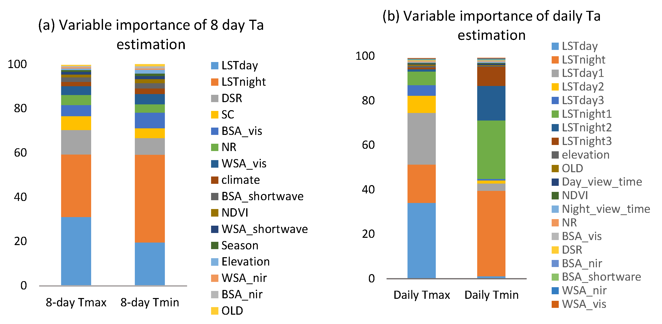
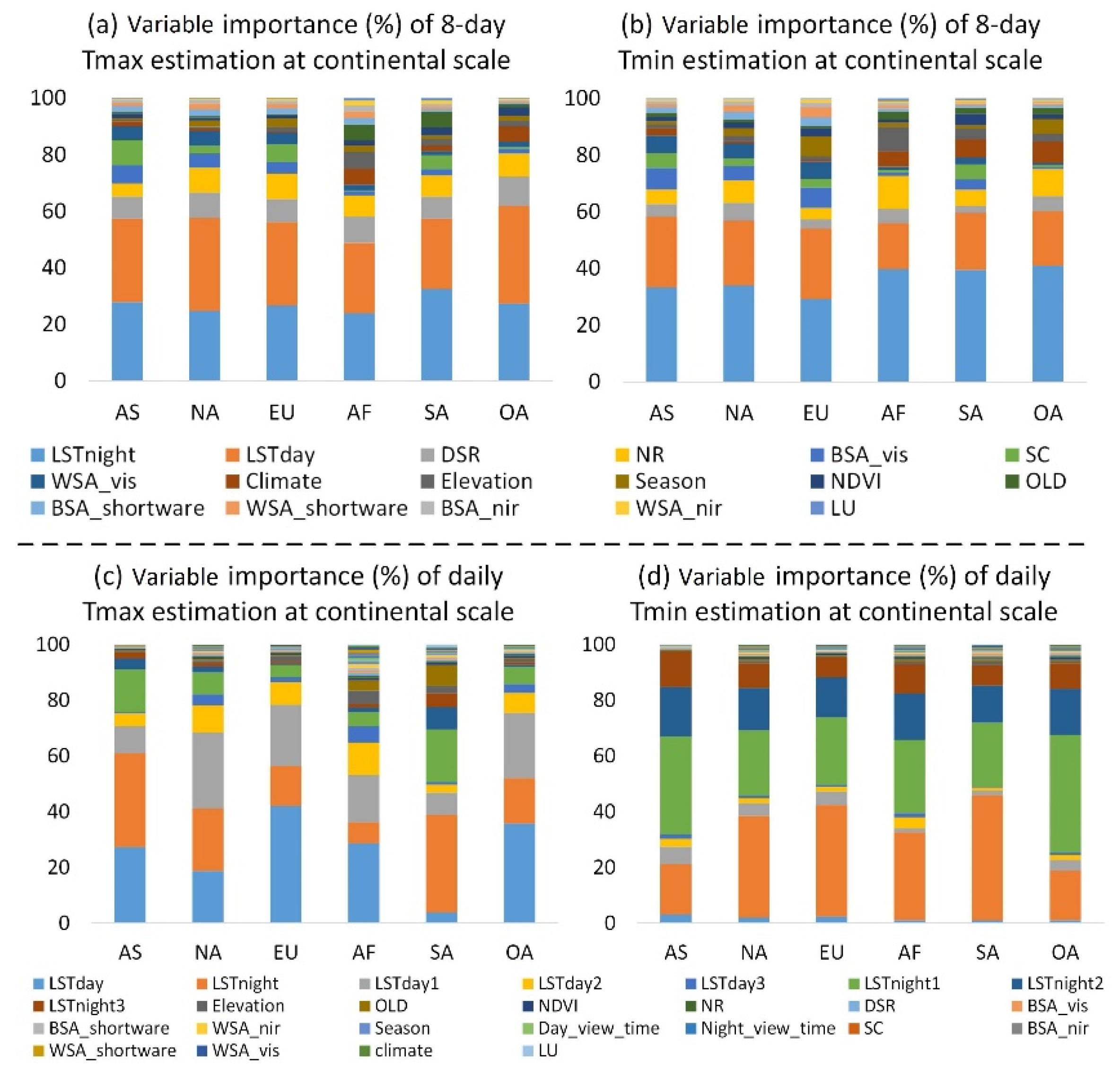
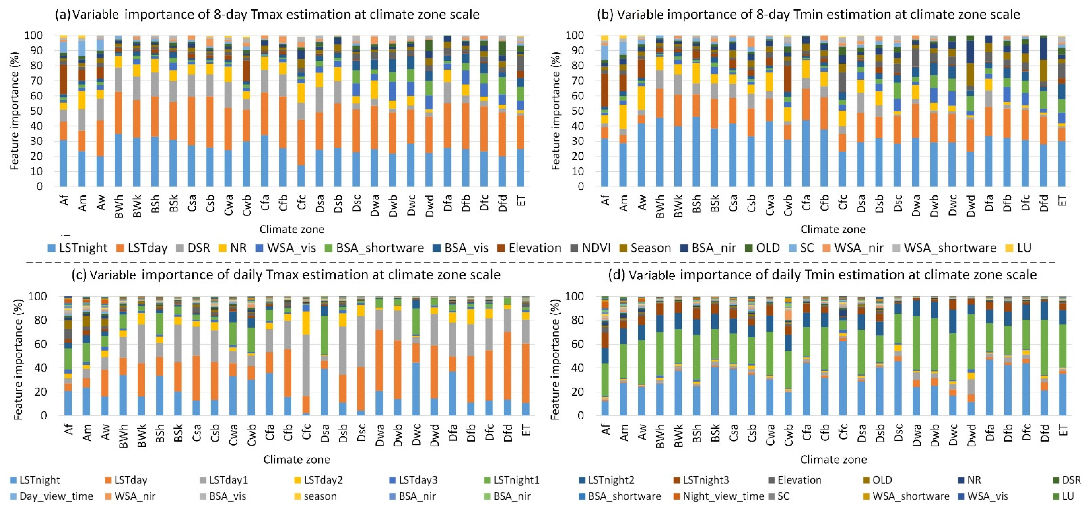
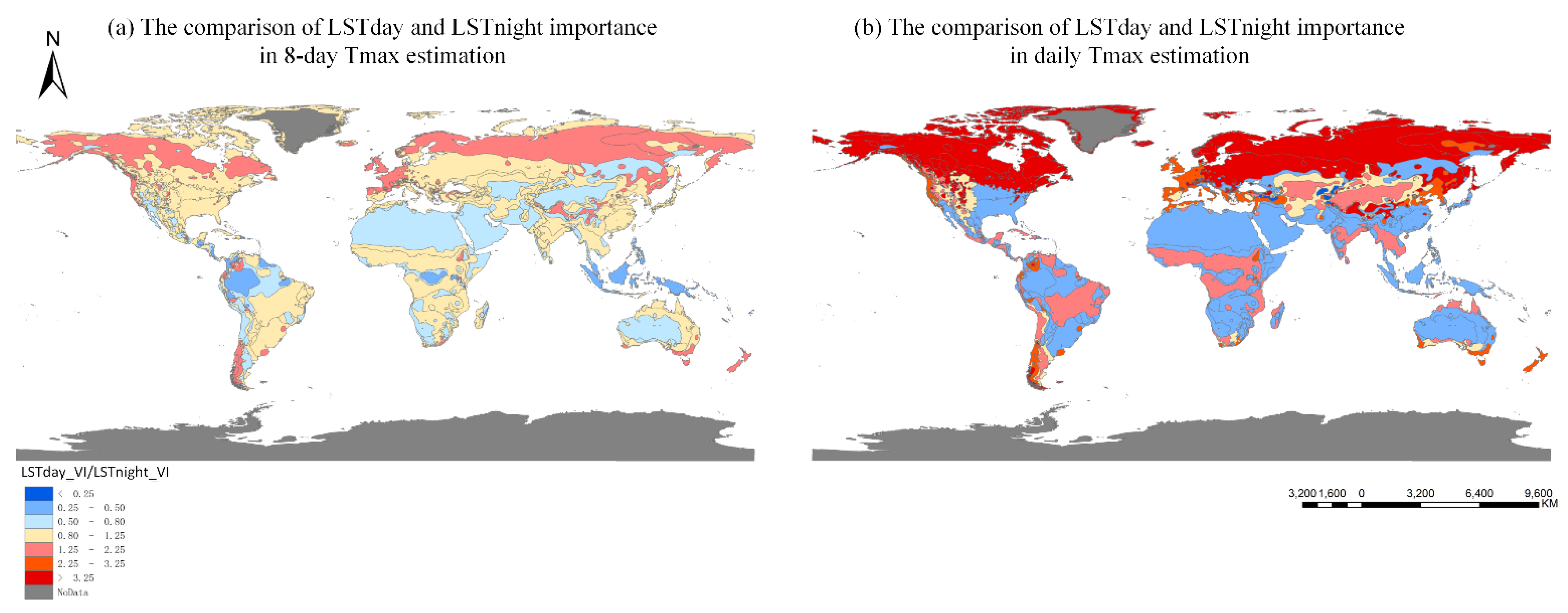
3.4. Variable Importance Analysis

Variable importance, as demonstrated and discussed in this section, indicates the contribution of the variables in Ta estimation at different temporal and spatial scales. It is expected to provide valuable references and improve our understanding of Ta estimation for the future. As there were few differences between the variable importance in spatial and temporal experiments (not shown), only the variable importance in the spatial experiments was presented in this study.

As shown in Figure 7, Figure 8 and Figure 9, the variable importance variations are different in estimation models at different temporal and spatial scales. On a global and continental scale, the two LST variables: LSTday and LSTnight account for about 60% totally in 8-day Tmax and Tmin estimation. While on a climate zone scale, both the contribution of LSTday and LSTnight varied with climate zones in 8-day Tmax estimation, ranging from 12% to 35%. In 8-day Tmin estimation, LSTnight played a more important role than LSTday in all the demonstrated climate zones, especially the tropical zone.

As for daily Tmax and Tmin estimation, the LST variables observed one to three days before estimation, especially LSTday1 or LSTnight1, made a significant contribution, as they are helpful to quantify the day-to-day changes of LST and identify the influence of turbulent flow exchange.

Considering daily Tmax estimation, the contribution of the eight LST variables varied significantly over space, ranging from 78% to 98% on a continental scale and ranging from 65% to 99% on a climate zone scale. LST variables had relatively higher contribution in daily Tmax estimation at cold zones, while they had less contribution in tropical zones where many other variables, especially OLD, influence and account for the daily Tmax estimation. As in the energy-limited condition, soil evaporation and plant transpiration have no clear cooling function when Ta is less than 5 °C [64], therefore many other variables, e.g., NR, NDVI, have little impact on the relationship between Ta and LST.

In daily Tmin estimation, the eight LST variables accounted for about 95% totally on global and continental scales, while they varied over different climate zones, ranging from 70% to 99%. LSTnight, as well as LSTnight1, LSTnight2 and LSTnight3, added overwhelming contributions, while LSTday, as well as LSTday1, LSTday2 and LSTday3, made little contribution.

However, the contribution of LSTnight1 varied with time and space. In North America, South America, and Europe, LSTnight made a higher contribution than LSTnight1. In Africa, LSTnight and LSTnight1 made a similar contribution. While, in Asia and Oceania, LSTnight1 made a clearly more significant contribution than LSTnight. Furthermore, LSTday1 contributed more to daily Tmax estimation than LSTday in the climate zones: Cfc, Dsb and Dsc, which indicates a delay of the energy balance establishment due to many ever-changing factors.

It is very interesting that the contributions of LSTday and LSTnight significantly varied over spatial and temporal scales. Compared to LSTnight, LSTday had a clearly higher importance on a global scale, as daily LST was an instantaneous observation and the time when LSTday was acquired was closer to the time when the Tmax was reached. However, the importance of LSTday and LSTnight can vary widely in different continents or climate zones for daily Tmax estimation. This was the reason why the previous studies had totally different results when comparing the models using LSTnight or LSTday in daily Tmax estimation at different study areas [36,37,38,39,40].

Figure 10 shows the spatial distribution of the importance ratio of LSTday and LSTnight on a climate zone scale for both 8-day and daily Tmax estimation. Compared to 8-day Tmax estimation, the difference between the importance of LSTday (LSTday_VI) and LSTnight (LSTnight_VI) changed more dramatically over the space in daily Tmax estimation. In 8-day Tmax estimation, LSTday and LSTnight had comparable contributions in many areas, e.g., the south of North America, the middle and east of South America, the south of Africa, the southeast of China, etc. In most of the remaining areas, LSTday had slightly higher or lower contributions than LSTnight. While as for the daily Tmax estimation, most of the areas experienced wide differences between LSTday_VI and LSTnight_VI. It is interesting that in daily Tmax estimation most of the areas located between 50 and 70 N^o, e.g., Canada and Russia, experienced much greater contributions from LSTday than LSTnight, while most of the other areas that located between 0 and 50 N^o and the southern hemisphere experienced much greater contributions from LSTnight than LSTday. This accords with the result for daily Tmax estimation in the Corn Belt of the United States conducted by Zeng et al. [4]. Zeng et al. [4] showed that the relationship between LSTday and Tmax is affected by several factors such as vegetation changes, land-cover types, soil moisture, etc., therefore, the areas with obvious vegetation seasonal changes, e.g., cropland (Corn Belt of US), and the arid zones (beginning with “B”) influenced by soil moisture, etc., experienced higher contribution from LSTnight than LSTday. While LSTnight tended to make a less significant contribution in the polar zones and cold zones except for Dsa, Dwc and Dfa.

Except for the LST variables, many other variables such as DSR, SC, NR made significant contributions in 8-day Ta estimation but had little contribution in daily Ta estimation. On a global and continental scale, except LSTday and LSTnight, DSR and NR contributed the most to 8-day Tmax estimation, and these two variables were also significant for 8-day Tmin estimation in most of the climate zones, except in the polar zones (ET) and some climate zones in cold zones, i.e., Dsc, Dwd, Dfb, Dfc, Dfd. In addition, snow cover had no small contribution in 8-day Tmax estimation at Asia, Europe, and South America or in 8-day Tmin estimation at Asia and South America. Elevation played a relatively high role than other variables except for LST variables in both 8-day Tmax and Tmin estimation of Africa. On a climate zone scale, elevation was also significant for 8-day Tmax estimation in the tropical zones (beginning with “A”) and a temperate zone: Cwb. OLD was important in the 8-day Tmax estimation for Africa and South America and in the 8-day Tmin estimation for South America. The season also made no small contribution to the 8-day Tmin estimation of Europe and Oceania.

As shown in Figure 7, Figure 8 and Figure 9, land cover contributed little in most of the climates. This seems to contradict other work (e.g., [31,33,65]) that confirmed the noticeable impacts of land cover on Tmax estimation as the specific heat varies significantly from one land cover type to another [31,33,65]. Nevertheless, Benali et al. [12] and Janatian et al. [32] indicated the independence of land cover when estimating Ta based on remote sensing data. This is possibly explained by the inclusion of the main factors reflecting the differences in land cover and the seasonality of the changes in vegetation, e.g., surface albedo and NDVI. The small land cover contribution in most of the climates also indicates that the main factors related to land cover difference in most of the climates were included in this study. In addition, MODIS land cover product itself includes uncertainty [32] and the static variables in machine learning-based models affect the model performance [34]. Thus, it is preferable to replace static variables such as land cover with dynamic variables to improve model performance.

3.5. Limitations and Future Studies

There are some limitations in this study that need to be further studied in the future. Firstly, we demonstrated the differences in Ta estimation accuracy and the influencing factors in different areas on a global scale. However, it is still difficult to explain them through the underlying mechanisms, the influence of climatic and environmental processes. In the future work, we will investigate and integrate this knowledge in the models to understand the difference of the estimation accuracy in different areas and provide further references to improve Ta estimation accuracy. Secondly, we did not have the opportunity to explore the uncertainties of the included variables on a global scale and to what extent the uncertainties influence the Ta estimation accuracy in different areas, especially for LST as the most important variable for Ta estimation based on remotely sensed data. LST observations are usually affected by undetected clouds, topography, and the split-window algorithm [57,66]. Thin or sub-pixel cloud clover is difficult to detect, especially for low-resolution sensors such as MODIS [12,16,61,67,68]. The error in MODIS LST due to cloud contamination and heavy aerosols can be very large (3–7 °C) [69]. For example, what is the reason for the inferior Ta estimation accuracy in some areas, low accuracy of LST retrievals, the complexity of the relationship between LST and Ta, or the absence of some important influencing factors? It is necessary to separate the uncertainty of included variables themselves from the used model itself in the future, which will provide valuable information for further improvement of model performance.

4. Conclusions

In this study, an RF model was applied based on an analysis of the physical relationship between Ta above the ground and LST observed from satellites. The model was validated on a “temporal” basis as well as a “spatial” basis. Both 8-day and daily Tmax and Tmin were estimated on a global, continental and climate zone scale through spatial and temporal experiments. The RF method shows great potential for mapping both 8-day and daily Tmax and Tmin, especially considering the high heterogeneity in land-cover types and topography on a global scale. The efficiency of the RF method displayed no indications of overtraining.

In this study, it was shown that the accuracy of Ta estimation varied with space and time in both the temporal and spatial experiments. On a global scale, higher accuracy was achieved in 8-day Ta estimations than was achieved in daily Ta estimations (R² > 0.96 and RMSE < 2 °C against R² > 0.95 and RMSE = 2.31~2.55 °C). On a continental scale, the RF method generally obtained high accuracy results for 8-day Tmax and Tmin estimation with R² > 0.9 and RMSE < 2 °C in temporal experiments and R² > 0.9 and RMSE~2 °C in spatial experiments, but delivered an inferior performance with R² > 0.8 and RMSE < 2.8 °C except for Africa for daily Tmax and Tmin estimations. On a climate zone scale, model accuracy with R² > 0.9 and RMSE < 3 °C and R² > 0.85 and RMSE < 3.5 °C was achieved for 8-day and daily Ta estimations in both the temporal and spatial experiments of the included climate zones.

The model was also trained and cross-validated at each spatial scale. The results showed that both the 8-day and daily Ta estimation accuracies using the continental model were higher than those using the global model in terms of RMSE, while both the 8-day and daily Ta estimation accuracies using climate zone models were lower than those using the global model in most of the climate zones. The data size and station distribution of the study area were the main factors influencing the model performance at different spatial scales.

Variable importance was analyzed after the application of the RF model. LST variables made overwhelming contributions in all the estimation models. LSTday and LSTnight made comparable contributions in 8-day Tmax estimations on a global and continental scale. LSTnight contributed more than LSTday in the 8-day Tmin estimation, though LSTday also contributed significantly in estimates for most of the climate zones. In daily Tmax estimations, the contributions of LSTday and LSTnight varied with space; nevertheless, LSTnight played an important role in the daily Tmax estimation, and it was often overlooked in previous studies. LSTday made little contribution to daily Tmin estimations in most of the climate zones. Except for LST variables, many other variables played important roles in Ta estimation, e.g., radiation-related variables, elevation, OLD, and season.

References

1. Montgomery, R.A.; Rice, K.E.; Stefanski, A.; Rich, R.L.; Reich, P.B. Phenological responses of temperate and boreal trees to warming depend on ambient spring temperatures, leaf habit, and geographic range. Proc. Natl. Acad. Sci. USA 2020, 117, 10397–10405. [Google Scholar] [CrossRef]
2. Allen, R. Penman–Monteith equation. In Encyclopedia of Soils in the Environment; Hillel, D., Ed.; Elsevier: Oxford, UK, 2005; pp. 180–188. [Google Scholar]
3. Zeng, L.; Wardlow, B.D.; Wang, R.; Shan, J.; Tadesse, T.; Hayes, M.J.; Li, D. A hybrid approach for detecting corn and soybean phenology with time-series MODIS data. Remote Sens. Environ. 2016, 181, 237–250. [Google Scholar] [CrossRef]
4. Zeng, L.; Brian, W.; Tsegaye, T.; Shan, J.; Michael, H.; Li, D.; Xiang, D. Estimation of daily air temperature based on modis land surface temperature products over the corn belt in the US. Remote Sens. 2015, 7, 951–970. [Google Scholar] [CrossRef] [Green Version]
5. Zhu, W.; Lű, A.; Jia, S. Estimation of daily maximum and minimum air temperature using MODIS land surface tempera-ture products. Remote Sens. Environ. 2013, 130, 62–73. [Google Scholar] [CrossRef]
6. Meyer, H.; Schmidt, J.; Detsch, F.; Nauss, T. Hourly gridded air temperatures of South Africa derived from MSG SEVIRI. Int. J. Appl. Earth Obs. Geoinf. 2019, 78, 261–267. [Google Scholar] [CrossRef]
7. Rao, Y.; Liang, S.; Wang, D.; Yu, Y.; Song, Z.; Zhou, Y.; Shen, M.; Xu, B. Estimating daily average surface air temperature using satellite land surface temperature and top-of-atmosphere radiation products over the Tibetan Plateau. Remote Sens. Environ. 2019, 234, 111462. [Google Scholar] [CrossRef]
8. Hooker, J.; Duveiller, G.; Cescatti, A. A global dataset of air temperature derived from satellite remote sensing and weather stations. Sci. Data 2018, 5, 180246. [Google Scholar] [CrossRef] [PubMed] [Green Version]
9. Zhu, W.; Lű, A.; Jia, S.; Yan, J.; Mahmood, R. Retrievals of all-weather daytime air temperature from MODIS products. Remote Sens. Environ. 2017, 189, 152–163. [Google Scholar] [CrossRef]
10. Shen, H.; Jiang, Y.; Li, T.; Cheng, Q.; Zeng, C.; Zhang, L. Deep learning-based air temperature mapping by fusing remote sensing, station, simulation and socioeconomic data. Remote Sens. Environ. 2020, 240, 111692. [Google Scholar] [CrossRef] [Green Version]
11. Lin, S.; Moore, N.J.; Messina, J.P.; Devisser, M.H.; Wu, J. Evaluation of estimating daily maximum and minimum air tem-perature with MODIS data in east Africa. Int. J. Appl. Earth Obs. Geoinf. 2012, 18, 140. [Google Scholar] [CrossRef]
12. Benali, A.; Carvalho, A.C.; Nunes, J.; Carvalhais, N.; Santos, A. Estimating air surface temperature in Portugal using MODIS LST data. Remote Sens. Environ. 2012, 124, 108–121. [Google Scholar] [CrossRef]
13. Chen, X.; Su, Z.; Ma, Y.; Middleton, E.M. Optimization of a remote sensing energy balance method over different canopy applied at global scale. Agric. For. Meteorol. 2019, 279, 107633. [Google Scholar] [CrossRef]
14. Nemani, R.R.; Running, S.W. Estimation of Regional Surface Resistance to Evapotranspiration from NDVI and Thermal-IR AVHRR Data. J. Appl. Meteorol. 1989, 28, 276–284. [Google Scholar] [CrossRef]
15. Prihodko, L.; Goward, S.N. Estimation of air temperature from remotely sensed surface observations. Remote Sens. Environ. 1997, 60, 335–346. [Google Scholar] [CrossRef]
16. Stisen, S.; Sandholt, I.; Rgaard, A.N.; Fensholt, R.; Eklundh, L. Estimation of diurnal air temperature using MSG SEVIRI data in West Africa. Remote Sens. Environ. 2007, 110, 262–274. [Google Scholar] [CrossRef]
17. Vancutsem, C.; Ceccato, P.; Dinku, T.; Connor, S.J. Evaluation of MODIS land surface temperature data to estimate air temperature in different ecosystems over Africa. Remote Sens. Environ. 2010, 114, 449–465. [Google Scholar] [CrossRef]
18. Sun, Y.; Wang, J.; Zhang, R.; Gillies, R.; Xue, Y.; Bo, Y. Air temperature retrieval from remote sensing data based on ther-modynamics. Theor. Appl. Climatol. 2005, 80, 37–48. [Google Scholar] [CrossRef]
19. Zhu, S.; Zhou, C.; Zhang, G.; Zhang, H.; Hua, J. Preliminary verification of instantaneous air temperature estimation for clear sky conditions based on SEBAL. Theor. Appl. Clim. 2017, 129, 71–81. [Google Scholar] [CrossRef]
20. Mostovoy, G.V.; King, R.L.; Reddy, K.R.; Kakani, V.G.; Filippova, M.G. Statistical Estimation of Daily Maximum and Minimum Air Temperatures from MODIS LST Data over the State of Mississippi. GIScience Remote Sens. 2006, 43, 78–110. [Google Scholar] [CrossRef] [Green Version]
21. Phan, T.; Degener, J.; Kappas, M. Comparison of multiple linear regression, cubist regression, and random forest algo-rithms to estimate daily air surface temperature from dynamic combinations of MODIS LST Data. Remote Sens. 2017, 9, 398. [Google Scholar]
22. Kloog, I.; Nordio, F.; Coull, B.A.; Schwartz, J. Predicting spatiotemporal mean air temperature using MODIS satellite sur-face temperature measurements across the Northeastern USA. Remote Sens. Environ. 2014, 150, 132–139. [Google Scholar] [CrossRef]
23. Yang, Y.Z.; Cai, W.H.; Yang, J. Evaluation of MODIS land surface temperature data to estimate near-surface air temperature in Northeast China. Remote Sens. 2017, 9, 410. [Google Scholar] [CrossRef] [Green Version]
24. Lu, N.; Liang, S.; Huang, G.; Qin, J.; Yao, L.; Wang, D.; Yang, K. Hierarchical Bayesian space-time estimation of monthly maximum and minimum surface air temperature. Remote Sens. Environ. 2018, 211, 48–58. [Google Scholar] [CrossRef]
25. Meyer, H.; Katurji, M.; Appelhans, T.; Ller, M.U.; Nauss, T.; Roudier, P.; Zawar-Reza, P. Mapping daily air temperature for Antarctica based on MODIS LST. Remote Sens. 2016, 8, 732. [Google Scholar] [CrossRef] [Green Version]
26. dos Santos, R.S. Estimating spatio-temporal air temperature in London (UK) using machine learning and earth observation satellite data. Int. J. Appl. Earth Obs. Geoinf. 2020, 88, 102066. [Google Scholar] [CrossRef]
27. Ho, H.C.; Knudby, A.; Sirovyak, P.; Xu, Y.; Hodul, M.; Henderson, S.B. Mapping maximum urban air temperature on hot summer days. Remote Sens. Environ. 2014, 154, 38–45. [Google Scholar] [CrossRef]
28. Yoo, C.; Im, J.; Park, S.; Quackenbush, L.J. Estimation of daily maximum and minimum air temperatures in urban landscapes using MODIS time series satellite data. ISPRS J. Photogramm. 2018, 137, 149–162. [Google Scholar] [CrossRef]
29. Jang, J.-D.; Viau, A.A.; Anctil, F. Neural network estimation of air temperatures from AVHRR data. Int. J. Remote Sens. 2004, 25, 4541–4554. [Google Scholar] [CrossRef]
30. Oyler, J.W.; Ballantyne, A.; Jencso, K.; Sweet, M.; Running, S.W. Creating a topoclimatic daily air temperature dataset for the conterminous United States using homogenized station data and remotely sensed land skin temperature. Int. J. Clim. 2015, 35, 2258–2279. [Google Scholar] [CrossRef]
31. Shen, S.; Leptoukh, G.G. Estimation of surface air temperature over central and eastern Eurasia from MODIS land surface temperature. Environ. Res. Lett. 2011, 6, 45206. [Google Scholar] [CrossRef]
32. Janatian, N.; Sadeghi, M.; Sanaeinejad, S.H.; Bakhshian, E.; Farid, A.; Hasheminia, S.M.; Ghazanfari, S. A statistical framework for estimating air temperature using MODIS land surface temperature data. Int. J. Clim. 2017, 37, 1181–1194. [Google Scholar] [CrossRef]
33. Cai, Y.; Chen, G.; Wang, Y.; Li, Y. Impacts of Land Cover and Seasonal Variation on Maximum Air Temperature Estima-tion Using MODIS Imagery. Remote Sens. 2017, 9, 233. [Google Scholar] [CrossRef] [Green Version]
34. Marzban, F.; Meteorologie, F.U.B.I.F.; Conrad, T.; Marzban, P.; Sodoudi, S. Estimation of the Near-Surface Air Temperature during the Day and Nighttime from MODIS in Berlin, Germany. Int. J. Adv. Remote Sens. GIS 2018, 7, 2478–2517. [Google Scholar] [CrossRef]
35. Zhang, W.; Huang, Y.; Yu, Y.; Sun, W. Empirical models for estimating daily maximum, minimum and mean air tempera-tures with MODIS land surface temperatures. Int. J. Remote Sens. 2011, 32, 9415–9440. [Google Scholar] [CrossRef]
36. Didari, S.; Zand-Parsa, S. Enhancing estimation accuracy of daily maximum, minimum, and mean air temperature using spatio-temporal ground-based and remote-sensing data in southern Iran. Int. J. Remote Sens. 2018, 39, 6316–6339. [Google Scholar] [CrossRef]
37. Mira, M.; Ninyerola, M.; Batalla, M.; Pesquer, L.; Pons, X. Improving mean minimum and maximum month-to-month air temperature surfaces using satellite-derived land surface temperature. Remote Sens. 2017, 9, 1313. [Google Scholar] [CrossRef] [Green Version]
38. Lee, M.H.; Yu, J.H.; Yun, H.; Cheon, E. Development of daily maximum air temperature estimation algorithm for the Korean peninsula using modis data. In Proceedings of the IGARSS 2018—2018 IEEE International Geoscience and Remote Sensing Symposium, Valencia, Spain, 22–27 July 2018; pp. 2555–2558. [Google Scholar]
39. Phan, T.; Kappas, M.; Degener, J. Estimating daily maximum and minimum land air surface temperature using modis land surface temperature data and ground truth data in Northern Vietnam. Remote Sens. 2016, 8, 1002. [Google Scholar]
40. Phan, T.N.; Kappas, M.; Nguyen, K.T.; Tran, T.P.; Tran, Q.V.; Emam, A.R. Evaluation of MODIS land surface temperature products for daily air surface temperature estimation in northwest Vietnam. Int. J. Remote Sens. 2019, 40, 5544–5562. [Google Scholar] [CrossRef]
41. Schwingshackl, C.; Hirschi, M.; Seneviratne, S.I. Quantifying spatiotemporal variations of soil moisture control on surface energy balance and near-surface air temperature. J. Clim. 2017, 30, 7105–7124. [Google Scholar] [CrossRef]
42. Beck, H.E.; Zimmermann, N.E.; McVicar, T.; Vergopolan, N.; Berg, A.; Wood, E.F. Present and future Köppen-Geiger climate classification maps at 1-km resolution. Sci. Data 2018, 5, 180214. [Google Scholar] [CrossRef] [PubMed] [Green Version]
43. GHCN Dataset from NOAA. Available online: https://www.ncdc.noaa.gov/ (accessed on 15 May 2021).
44. Rabus, B.; Eineder, M.; Roth, A.; Bamler, R. The shuttle radar topography mission—a new class of digital elevation models acquired by spaceborne radar. ISPRS J. Photogramm. Remote Sens. 2003, 57, 241–262. [Google Scholar] [CrossRef]
45. Yan, H.; Zhang, J.; Hou, Y.; He, Y. Estimation of air temperature from MODIS data in east China. Int. J. Remote Sens. 2009, 30, 6261–6275. [Google Scholar] [CrossRef]
46. Xu, Y.; Qin, Z.; Shen, Y. Study on the estimation of near-surface air temperature from MODIS data by statistical methods. Int. J. Remote Sens. 2012, 33, 7629–7643. [Google Scholar] [CrossRef]
47. Sohrabinia, M.; Zawar-Reza, P.; Rack, W. Spatio-temporal analysis of the relationship between LST from MODIS and air temperature in New Zealand. Theor. Appl. Clim. 2015, 119, 567–583. [Google Scholar] [CrossRef]
48. Timmermans, W.J.; Kustas, W.P.; Anderson, M.C.; French, A.N. An intercomparison of the Surface Energy Balance Algorithm for Land (SEBAL) and the Two-Source Energy Balance (TSEB) modeling schemes. Remote Sens. Environ. 2007, 108, 369–384. [Google Scholar] [CrossRef]
49. Jiang, L.; Islam, S. An intercomparison of regional latent heat flux estimation using remote sensing data. Int. J. Remote Sens. 2003, 24, 2221–2236. [Google Scholar] [CrossRef]
50. Lin, X.; Zhang, W.; Huang, Y.; Sun, W.; Han, P.; Yu, L.; Sun, F. Empirical estimation of near-surface air temperature in China from MODIS LST Data by considering physiographic features. Remote Sens. 2016, 8, 629. [Google Scholar] [CrossRef] [Green Version]
51. Roerink, G.; Su, Z.; Menenti, M. S-SEBI: A simple remote sensing algorithm to estimate the surface energy balance. Phys. Chem. Earth Part B Hydrol. Oceans Atmos. 2000, 25, 147–157. [Google Scholar] [CrossRef]
52. Malbéteau, Y.; Parkes, S.; Aragon, B.; Rosas, J.; McCabe, M.F. Capturing the diurnal cycle of land surface temperature using an unmanned aerial vehicle. Remote Sens. 2018, 10, 1407. [Google Scholar] [CrossRef] [Green Version]
53. Kattel, D.B.; Yao, T.; Ullah, K.; Rana, A.S. Seasonal near-surface air temperature dependence on elevation and geographical coordinates for Pakistan. Theor. Appl. Climatol. 2019, 138, 1591–1613. [Google Scholar] [CrossRef]
54. Wild, M.; Folini, D.; Hakuba, M.Z.; Schär, C.; Seneviratne, S.I.; Kato, S.; Rutan, D.; Ammann, C.; Wood, E.F.; König-Langlo, G. The energy balance over land and oceans: An assessment based on direct observations and CMIP5 climate models. Clim. Dyn. 2014, 44, 3393–3429. [Google Scholar] [CrossRef] [Green Version]
55. Li, L.; Zha, Y. Mapping relative humidity, average and extreme temperature in hot summer over China. Sci. Total Environ. 2018, 615, 875–881. [Google Scholar] [CrossRef]
56. Zeng, L.; Hu, S.; Xiang, D.; Zhang, X.; Li, D.; Li, L.; Zhang, T. Multilayer soil moisture mapping at a regional scale from multisource data via a machine learning method. Remote Sens. 2019, 11, 284. [Google Scholar] [CrossRef] [Green Version]
57. Chen, F.; Liu, Y.; Liu, Q.; Qin, F. A statistical method based on remote sensing for the estimation of air temperature in China. Int. J. Clim. 2014, 35, 2131–2143. [Google Scholar] [CrossRef]
58. Moser, G.; De Martino, M.; Serpico, S.B. Estimation of Air Surface Temperature from Remote Sensing Images and Pixelwise Modeling of the Estimation Uncertainty Through Support Vector Machines. IEEE J. Sel. Top. Appl. Earth Obs. Remote Sens. 2015, 8, 332–349. [Google Scholar] [CrossRef]
59. Khesali, E.; Mobasheri, M. A method in near-surface estimation of air temperature (NEAT) in times following the satellite passing time using MODIS images. Adv. Space Res. 2020, 65, 2339–2347. [Google Scholar] [CrossRef]
60. Mutiibwa, D.; Strachan, S.; Albright, T. Land Surface Temperature and Surface Air Temperature in Complex Terrain. IEEE J. Sel. Top. Appl. Earth Obs. Remote Sens. 2015, 8, 4762–4774. [Google Scholar] [CrossRef]
61. Emamifar, S.; Rahimikhoob, A.; Noroozi, A.A. Daily mean air temperature estimation from MODIS land surface temper-ature products based on M5 model tree. Int. J. Climatol. 2013, 33, 3174–3181. [Google Scholar] [CrossRef]
62. Pleim, J.E. A simple, efficient solution of flux–Profile relationships in the atmospheric surface layer. J. Appl. Meteorol. Clim. 2006, 45, 341–347. [Google Scholar] [CrossRef]
63. Hughes, M.; Hall, A.; Fovell, R.G. Dynamical controls on the diurnal cycle of temperature in complex topography. Clim. Dyn. 2007, 29, 277–292. [Google Scholar] [CrossRef]
64. Sun, Z.; Wang, Q.; Batkhishig, O.; Ouyang, Z. Relationship between evapotranspiration and land surface temperature under energy- and water-limited conditions in dry and cold climates. Adv. Meteorol. 2016, 2016, 1–9. [Google Scholar] [CrossRef] [Green Version]
65. Peón, J.; Recondo, C.; Calleja, J.F. Improvements in the estimation of daily minimum air temperature in peninsular Spain using MODIS land surface temperature. Int. J. Remote Sens. 2014, 35, 5148–5166. [Google Scholar] [CrossRef]
66. Zhang, H.; Zhang, F.; Zhang, G.; Ma, Y.; Yang, K.; Ye, M. Daily air temperature estimation on glacier surfaces in the Tibetan Plateau using MODIS LST data. J. Glaciol. 2018, 64, 132–147. [Google Scholar] [CrossRef] [Green Version]
67. Ackerman, S.; Strabala, K.I.; Menzel, W.P.; Frey, R.A.; Moeller, C.C.; Gumley, L.E. Discriminating clear sky from clouds with MODIS. J. Geophys. Res. Space Phys. 1998, 103, 32141–32157. [Google Scholar] [CrossRef]
68. Jin, M.S.; Dickinson, R.E. Land surface skin temperature climatology: Benefitting from the strengths of satellite observations. Environ. Res. Lett. 2010, 5, 44004. [Google Scholar] [CrossRef] [Green Version]
69. Wan, Z.; Li, Z. Radiance-based validation of the V5 MODIS land-surface temperature product. Int. J. Remote Sens. 2008, 29, 5373–5395. [Google Scholar] [CrossRef]
Figure 1. Spatial distribution of the meteorological stations used in this study.
Remotesensing 13 02355 g001
Figure 2. The framework design of this study.
Remotesensing 13 02355 g002
Figure 3. Estimation accuracy, i.e., R2 and RMSE, of 8-day (a,c) and daily (b,d) Tmax and Tmin in both spatial and temporal experiments on a continental scale: Asia (AS), North America (NA), Europe (EU), Africa (AF), South America (SA), Oceania (OA).
Remotesensing 13 02355 g003
Figure 4. Estimation accuracy, i.e., R2 and RMSE, of 8-day (a,c) and daily (b,d) Tmax and Tmin in both spatial and temporal experiments on a climate zone scale.
Remotesensing 13 02355 g004
Figure 5. The averaged cross-validated estimation accuracy of 8-day (a,c) and daily (b,d) Ta in spatial experiments using the models trained at global and continental scale (a,b) or global and climate zone scale. Global/Continental/Climate -8 day/daily-Tmax/Tmin means using the model for 8-day/daily Tmax/Tmin estimation trained on a global, continental and climate zone scale (corresponding continents or climate zone), respectively.
Remotesensing 13 02355 g005
Figure 6. Spatial patterns of the 8-day and daily Tmax and Tmin estimation model performance at the different spatial patterns in spatial experiments.
Remotesensing 13 02355 g006
Figure 7. Variable importance (%) of 8-day (a) and daily (b) Tmax and Tmin in spatial experiments on a global scale.
Remotesensing 13 02355 g007
Figure 8. Variable importance (%) of 8-day tmax (a), 8-day Tmin (b), daily Tmax (c), and daily Tmin (d) estimation in spatial experiments at a continental scale.
Remotesensing 13 02355 g008
Figure 9. Variable importance (%) of 8-day tmax (a), 8-day Tmin (b), daily Tmax (c), and daily Tmin (d) in spatial experiments on a climate zone scale.
Remotesensing 13 02355 g009
Figure 10. The spatial pattern of the variable importance comparison of LSTday (LSTday_VI) and LSTnight (LSTnight_VI) in 8-day Tmax (a) and daily Tmax estimation (b) based on the results on a climate zone scale. The color shows the variations of the ratio of LSTday_VI and LSTnight_VI.
Remotesensing 13 02355 g010