
Imputation of GPS Coordinate Time Series Using missForest


1
Chinese Antarctic Center of Surveying and Mapping, Wuhan University, Wuhan 430079, China
2
School of Geomatics Science and Technology, Nanjing Tech University, Nanjing 211800, China
3
Department of Land Surveying and Geo-Informatics, Hong Kong Polytechnic University, Kowloon, Hong Kong
*
Author to whom correspondence should be addressed.
Remote Sens. 2021, 13(12), 2312; https://doi.org/10.3390/rs13122312
Submission received: 12 May 2021
/
Revised: 8 June 2021
/
Accepted: 9 June 2021
/
Published: 12 June 2021
Abstract
:The global positioning system (GPS) can provide the daily coordinate time series to help geodesy and geophysical studies. However, due to logistics and malfunctioning, missing values are often “seen” in GPS time series, especially in polar regions. Acquiring a consistent and complete time series is the prerequisite for accurate and reliable statical analysis. Previous imputation studies focused on the temporal relationship of time series, and only a few studies used spatial relationships and/or were based on machine learning methods. In this study, we impute 20 Greenland GPS time series using missForest, which is a new machine learning method for data imputation. The imputation performance of missForest and that of four traditional methods are assessed, and the methods’ impacts on principal component analysis (PCA) are investigated. Results show that missForest can impute more than a 30-day gap, and its imputed time series has the least influence on PCA. When the gap size is 30 days, the mean absolute value of the imputed and true values for missForest is 2.71 mm. The normalized root mean squared error is 0.065, and the distance of the first principal component is 0.013. missForest outperforms the other compared methods. missForest can effectively restore the information of GPS time series and improve the results of related statistical processes, such as PCA analysis.
1. Introduction
Modern data measurement and acquisition consistently encounter the problem of missing data. For example, due to logistics and malfunctioning, missing values are often “seen” in GPS daily time series [1]. In particular, in polar regions with a harsh environment, logistics personnel cannot immediately deal with emerging GPS battery-/hardware-related problems; hence, cases of missing values are much more common in polar regions than in other regions. Regardless of the reason for the missing data, consistent and complete data are the prerequisite for an accurate and reliable statistical analysis. Most conventional time series analysis methods, such as wavelet transform [2], principal/independent component analysis [3,4,5], and spectrum analysis [6], require non-missing data. This requirement forces geodetic researchers who wish to perform further analysis of GPS time series to select between imputing or discarding missing data. Simply discarding missing data is not a reasonable practice because it would inevitably discard valuable information and/or compromise inferential power, especially for polar regions where GPS sites are rare. How to make full use of every dataset is of great importance. Data imputation, which focuses on the use of available information in existing data to impute missing data, is a more reasonable and practical approach than discarding missing data [7]. Here, we use the term “imputation” instead of the commonly used term “interpolation” in geodetic studies and adopt the definition that the former is meant to fill in missing values in the dataset, whereas the latter predicts values at unsampled locations [8].
Imputation of missing data is a crucial pre-processing step in GPS time series analysis. Dong et al. [4] used three-point Lagrange imputation to fill GPS daily time series with time gaps shorter than two days and iterative principal component analysis (PCA) algorithm for larger gaps. He et al. [5] used a third-order spline imputation method for time gaps shorter than three days and simple linear imputation for other gaps to maintain the original trend of GPS time series. Xu et al. [9] proposed a method based on iterative empirical orthogonal functions to reconstruct gappy GPS time series and confirmed that it is superior to the conventional least-squares method in the estimation of periodic amplitude in wavelet analysis. Wang et al. [10] proposed an imputation method based on singular spectrum analysis; their method does not need prior information and shows good performance when the missing rate is 20%. Liu et al. [1] introduced an imputation method based on the Kalman filter that can consider the spatial correlation between stations. The regulated expectation maximization (RegEM) proposed by Schneider et al. [11] was initially designed for meteorological data, and Li et al. [12] used it to impute GPS daily time series before spatiotemporal filtering and further analysis. The performance of these methods usually depends on the tuning parameters or specification of a parametric model [13] and makes assumptions about the data distribution, such as uniform or normal distribution [14]. These drawbacks mean that these imputation models must be appropriately specified for analyses based on imputed data [15]. Moreover, studies that used PCA, RegEM, and other spatial-related methods to impute GPS time series led to a new stage of considering the complex interactions and nonlinearity of variables, rather than just a standalone continuous variation changing with time [4,16]. An imputation algorithm that can consider the spatiotemporal changes in variables and make as few assumptions as possible about the structural aspects of data must be established to obtain unbiased and consistent spatiotemporal imputation results and avoid problematic situations.
A standout in the fields of computer vision and natural language processing, machine learning has strong modeling capability and can find the optimal model for the imputed data through iteration without a priori knowledge [17,18,19,20]. Many imputation applications are based on machine learning in the field of time series analysis. Cao et al. [21] proposed the bidirectional recurrent impact for time series methods based on the bidirectional recurrent neural network and spatial correlation. Yoon et al. [22] proposed a novel method called Generative Adversarial Imputation Nets (GAIN) for imputing missing data by adapting the well-known Generative Adversarial Nets (GAN) framework. Both methods show better performance than traditional ones in the multivariate time series imputation. In this study, we introduce an iterative imputation method (missForest) based on Breiman’s random forests [23]. missForest has desirable characteristics for imputation; namely, it (1) can address complex interactions and nonlinearity as a non-parametric method, (2) can handle mixed types of missing data and is easy to scale to high dimensions, even in cases where the number of variables exceeds the number of observations, and (3) does not need a priori knowledge about the original data but still provides excellent imputation results. The missForest algorithm, as an extended random forest algorithm, allows for estimating the so-called out-of-bag (OOB) error, which is the mean of squared differences between each observed value and the prediction, based on trees for which that observation is not included in the bootstrap sample. This feature offers missForest a means to assess its imputation quality without the need to set aside test data nor perform laborious cross-validations.
Given that the missForest algorithm meets all the characteristics for handling missing data and its effectiveness and robustness have been verified in many previous studies [24,25], using missForest to impute the missing data of GPS coordinate time series is reasonable and desirable. However, to our knowledge, little guidance has been provided about the performance of missForest compared with that of other traditional imputation algorithms for GPS time series in the literature. In this study, we assess the imputation performance of missForest and several state-of-the-art methods by using gappy GPS time series with artificially missing rates of up to ~40%. The OOB imputation error of missForest provides a good approximation of the true imputation error. PCA is also used to assess the imputation performance of missForest and other algorithms. The advantages and disadvantages of the imputation algorithms in maintaining the data structure are verified through the statistics on the variance percentage of the first three components to the total variance and the distance and angle of the first component between the imputed and original data. Through comparison and assessment, we aim to prove that missForest is a promising and easy-to-use imputation algorithm.
2. Methods and Data
2.1. missForest
missForest is an iterative imputation method based on random forest. By averaging many unpruned classification or regression trees, random forest intrinsically constitutes a multiple imputation scheme. By using the built-in OOB error estimates of random forest, missForest can estimate the imputation error without the need for a test set. In other comparative studies, missForest outperformed other methods of imputation, especially in data settings where complex interactions and nonlinear relations are suspected. The OOB error estimations of missForest are adequate in all settings. In this study, we verify the effectiveness of OOB in GPS time series imputation.
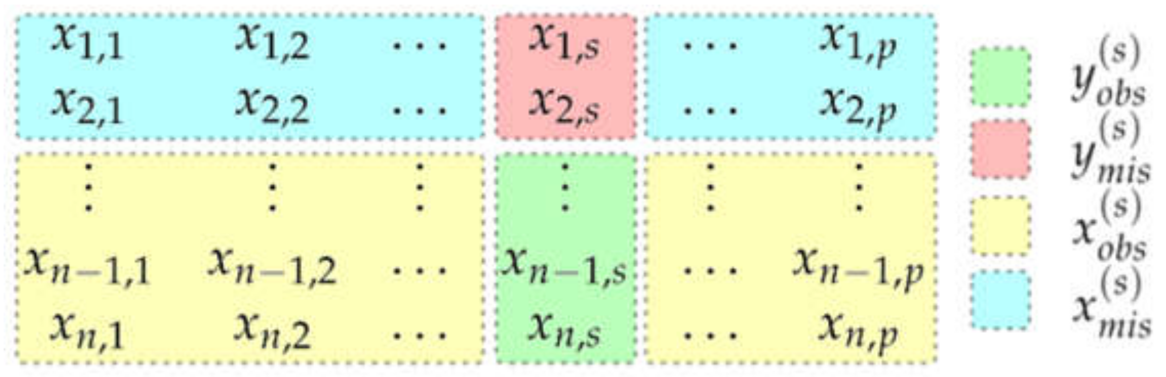
Let be an GPS coordinate matrix that requires imputation, that is,
where n is the total observation epochs of the time series and p is the number of GPS stations. Every variable that contains missing values at entries will divide into the following four parts (Figure 1).
- , the non-missing observed values of variable ;
- , the missing values of variable ;
- , the variable with observations other than ;
- , the variables with observations other than .
Notably, () are usually not completely observed (missing).
The imputation procedure of missForest begins with making an initial guess for the missing values in by using, for example, mean imputation, and by sorting the variables () according to their number of missing values from low to high. For each variable (), the missing values are imputed by training a random forest with responses () and predictors () and predicting the missing values () by applying the trained random forest to . This procedure is repeated until the difference (defined by Equation (2)) between the imputed matrix (), and the previous one () did not increase. Algorithm 1 gives a representation of the missForest method. In this study, the maximum iteration of the missForest is 10, and the number of trees is 100.
| Algorithm 1 missForest |
| Require: an matrix, stopping criterion 1: Sort by amount of missing values of stations descend; 2: Make an initial guess for missing values using another method; 3: while not do 4: store previously imputed matrix; 5: for s in do 6: Fit a random forest:; 7: Predict using ; 8: update impute matrix, using predicted ; 9: update 10: return the imputed matrix ; |
2.2. Baseline Methods
Several traditional imputation/interpolation methods of GPS time series are used as baseline methods for comparison to validate the performance of missForest. These methods are described below.
Cubic spline [26] is a form of imputation method that uses a special type of piecewise polynomial called spline. This method provides an imputing polynomial that is smoother and has a smaller error than several other imputing polynomials, such as Lagrange and Newton polynomials.
Orthogonal polynomial [27] imputation uses a family of polynomials to impute missing data, such that any two different polynomials in the sequence are orthogonal to each other under an inner product.
Hermite imputation [28] is an application of the Chinese remainder theorem for univariate polynomials that may involve moduli of arbitrary degrees (Lagrange imputation involves only moduli of degree one).
RegEM [11] neither depends on the data model nor introduces a priori information, but it relies on the self-characteristics of the data to impute the missing values while taking the physical background and the correlation of the time series into account. With GPS time series as an example, RegEM uses maximum likelihood estimation to estimate the linear relationship between different GPS stations. The linear relationship between stations can be expressed by Equation (3). is the time series, and is the predicted value. We can obtain by maximum likelihood (Equation (4)). In RegEM, ridge regression is introduced as a regularization term. Hence, we can derive related to (Equation (5)). We can find the best value by iteration and obtain reliable results. In this study, the maximum iteration of the RegEM process is 10 (the same iteration as missForest), and the multiple ridge regression is used.
Among the methods, cubic spline, orthogonal polynomial, and Hermite are based only on time correlation, whereas RegEM and missForest consider spatial correlation. Moreover, RegEM only considers the linear relationship between stations, whereas missForest can consider the nonlinear relationship between stations. The difference between RegEM and missForest is that missForest uses RandomForest but RegEM uses linear to fit the relationship of and .
2.3. Evaluation Indicators
The mean absolute error (MAE, Equation (6)) and normalized root mean squared error (NRMSE, Equation (7)) are used to evaluate the imputation performance of missForest and the baseline methods.
where and are the true and imputed matrixes, respectively. Mean and var denote empirical mean and variance notations, respectively. For NRMSE, the closer the value is to 0 (1), the better (worse) the imputation performance is.
missForest, as an extended random forest algorithm, allows for estimating the OOB error, which is the mean of squared differences between each observed value and the predicted value based on trees, for which that observation is not included in the bootstrap sample. Over many iterations, the OOB error produces a similar error estimate as cross-validation. That is, once the OOB error stabilizes, it converges to the cross-validation error. The advantage of the OOB method is that it requires minimal computation and allows model assessment as it is being trained. We compare the OOB error of missForest to that of NRMSE for all GPS time series and confirm that OOB, as the true imputation error, is an accurate and reliable indicator of imputation performance.
The Pearson correlation coefficient is used to measure the linear correlation between the interpolation result and the true value.
2.4. PCA
PCA is a widely used data analysis tool to reduce dimensionality and increase interpretability while minimizing information loss [29]. It is useful in exploratory data analysis and for building predictive models. In GPS time series analysis, PCA is often adopted as a spatiotemporal filter to eliminate common-mode errors (CME) [4]. PCA spatial filtering can extract CME more accurately and effectively than the conventional overall filtering method.
The n × m matrix represents the normalized daily coordinate time series of n sites and time spanning m days. We compute the variance–covariance matrix with equal weighting on every normalized coordinate time series. We let be the eigenvector and eigenvalue of , respectively. The symmetric matrix can be decomposed as where is an eigenvector matrix and 𝜦 is a diagonal matrix with eigenvalues of the data matrix ordered according to magnitude (sorted in descending order). Matrix can be given as = 𝑷, where is a matrix. The th row vector in is called the th principal component (PC) of the original data , and the th column vector in is its corresponding spatial responses. Matrix can be obtained by . The regional GPS coordinate time series can be expressed as the product of PCs and their spatial responses.
Given that , we determine that is the variance of the projection of the observation matrix on the eigenvector. , and we can derive the proportion of variance of the observation matrix in each eigenvector direction by using Equation (9). By comparing the between the raw and imputed time series, we can quantify the influence of different imputation methods on the original time series.
Let be the observation matrix after imputation and be the projection of the observation matrix on the principal component. We can obtain the distance of projection before and after imputation by applying Equation (10).
Through and, we can analyze the influence of imputation on PCA so that the advantages and disadvantages of the imputation algorithms in maintaining the data structure can be verified.
2.5. Out-of-Bag Error (OOB)
The OOB error, also known as the out-of-bag estimate, is a way of calculating the prediction error of random forests, boosted decision trees, and other machine learning models using bootstrap aggregation (bagging). Bagging creates training samples for the model learning by using subsampling with replacement. The OOB error is the mean prediction error in each training sample utilizing just the trees in the bootstrap sample that did not have data [30]. The OOB error is often used for assessing the prediction performance of RF and is often claimed to be an unbiased estimator for the true error. However, using out-of-bag error may overestimate the true prediction error depending on the choices of random forest parameters [31]. In our study, OOB is the estimated values of the NRMSE of real and imputed data. When a large deviation exists between OOB and NRMSE, the results of missForest are not credible. Therefore, we can use the true NRMSE to check the OOB and yield less biased estimates of the true prediction error.
2.6. GPS Time Series and Experiment Settings
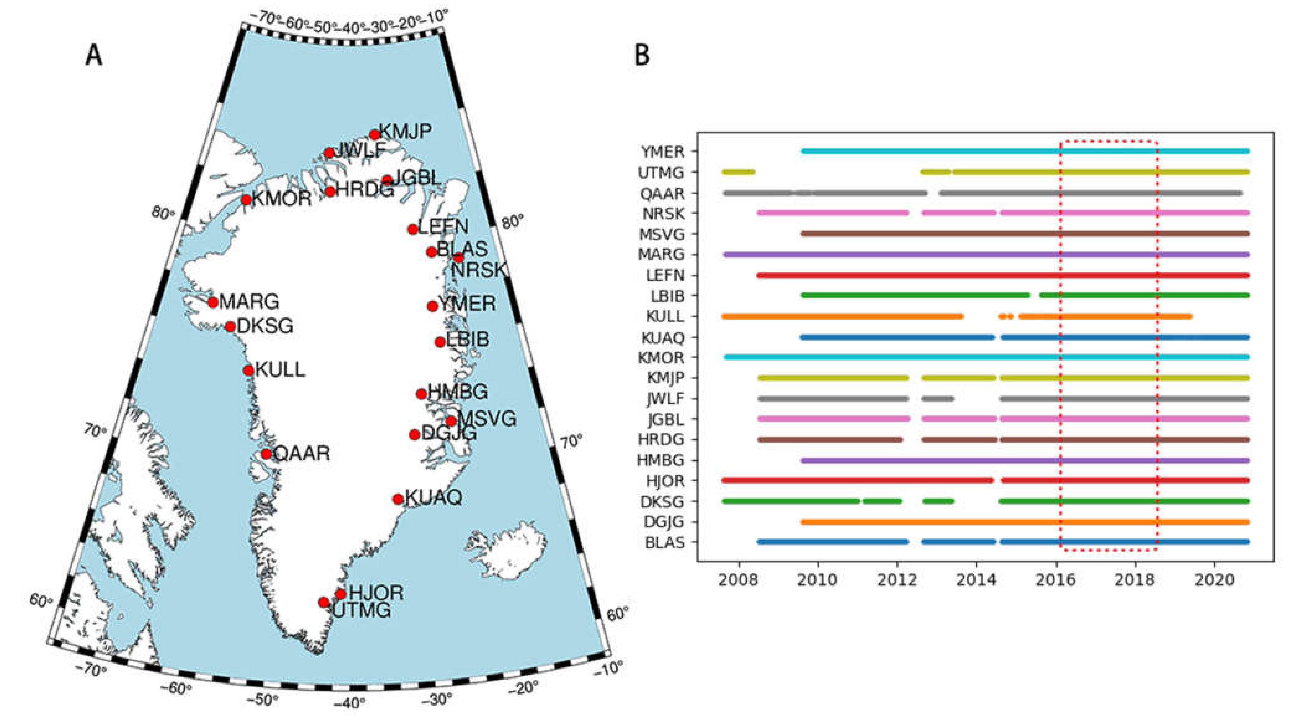
The GPS time series records used in this study are downloaded from the Nevada Geodetic Laboratory, the University of Nevada at Reno (http://geodesy.unr.edu/NGLStationPages/GlobalStationList, accessed at 12 May 2021) [32], and correspond to IGb2014 products. On the basis of the distribution and integrity of the GPS time series, we select 20 GPS stations in Greenland. Figure 2A shows the location of the 20 GPS stations, and Figure 2B shows the observation epochs of all sites. We focus on the vertical component of the GNSS coordinate time series. The average missing rate of all of the time series is 13.28%. We use time series from January 2016 to June 2018 because the time series of this period has no gaps.
3. Imputation Results
3.1. Different Gap Size Analysis
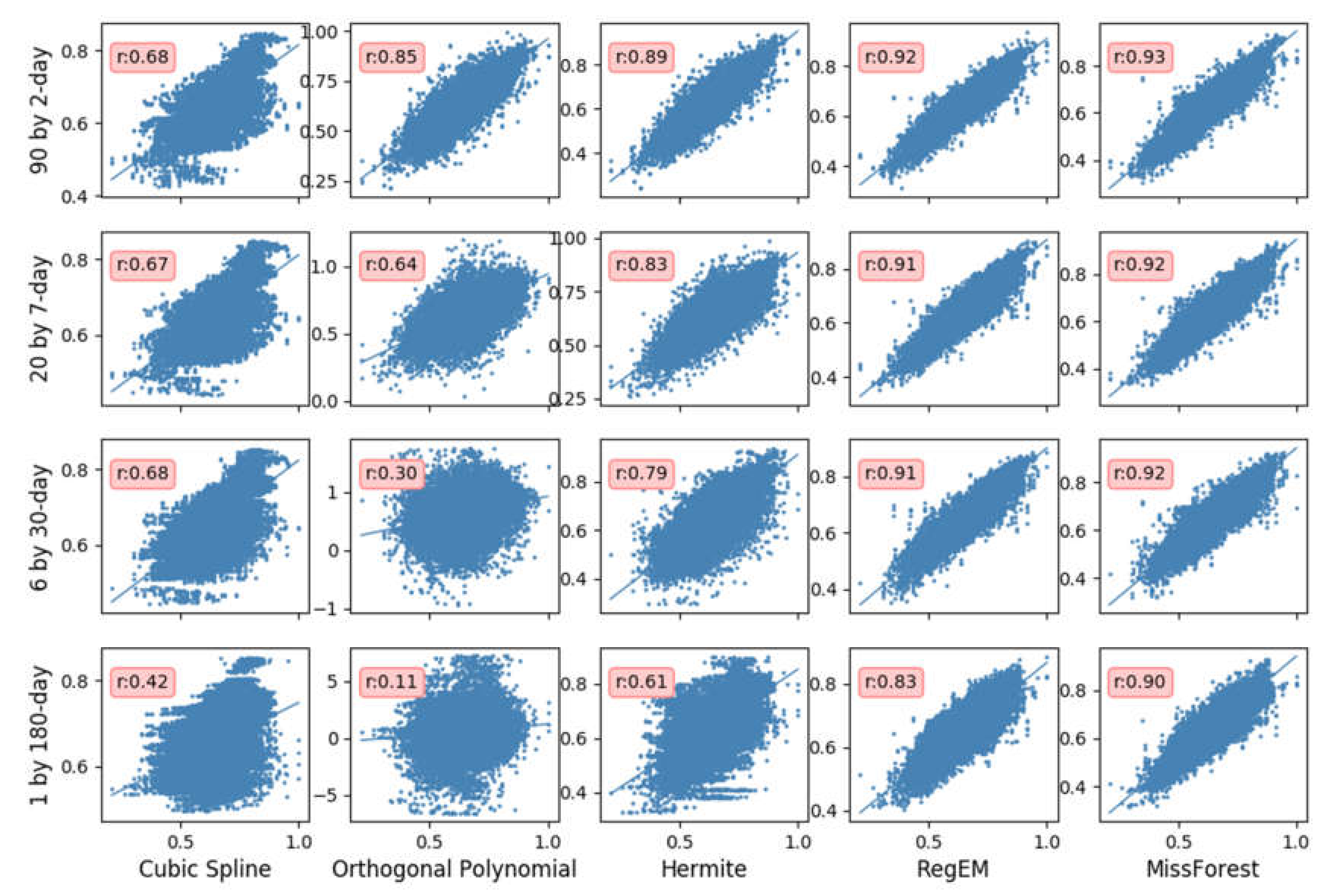
We use 20 GPS time series in Greenland from January 2016 to June 2018 as test datasets. We randomly remove (a) 90 by 2-day, (b) 20 by 7-day, (c) 6 by 30-day, and (d) 1 by 180-day data at ten random stations as gappy time series to perform the following analysis. To avoid the contingency of the experimental results, we conduct 200 random trials and average their MAE, NRMSE, and calculate one correlation coefficient (Rp) for all 200 trials together (Figure 3 and Table 1). Due to the range of sites, we regularize the time series to calculate the NRMSE and Rp (the following experiments are the same). When the gap size is 2 days, the 5 mm MAE of cubic spline is the largest, whereas the 2.55 mm MAE of missForest is the smallest. The Rp of all the methods is better than 0.68. We can conclude from Figure 3 that RegEM and missForest have the best correlation with the true values, and the three other methods show large dispersion. When the gap size increases to 7 days, the results of orthogonal polynomial worsen, and its MAE and NRMSE values increase to 6.27 and 0.152, respectively. Hermite also exhibits some degradation. Meanwhile, missForest is more stable than the Hermite and orthogonal polynomial. When the gap size is 30 days, cubic spline and orthogonal polynomial become unstable, and the Rp of the orthogonal polynomial is less than 0.3, indicating that the differences between the imputed and true values increase with increasing gap size. When the gap size is 180 days, the results of RegEM and missForest change little with respect to the 2-day results, indicating that considering the spatial correlation makes the imputation results more robust to gap size than those of temporal-only correlation methods. The larger the gap is, the lower the temporal correlation is. missForest has stronger modeling capabilities (e.g., to address complex interactions and nonlinearity) than RegEM, and the results of missForest are the best overall.
3.1.1. 2-Day Gap
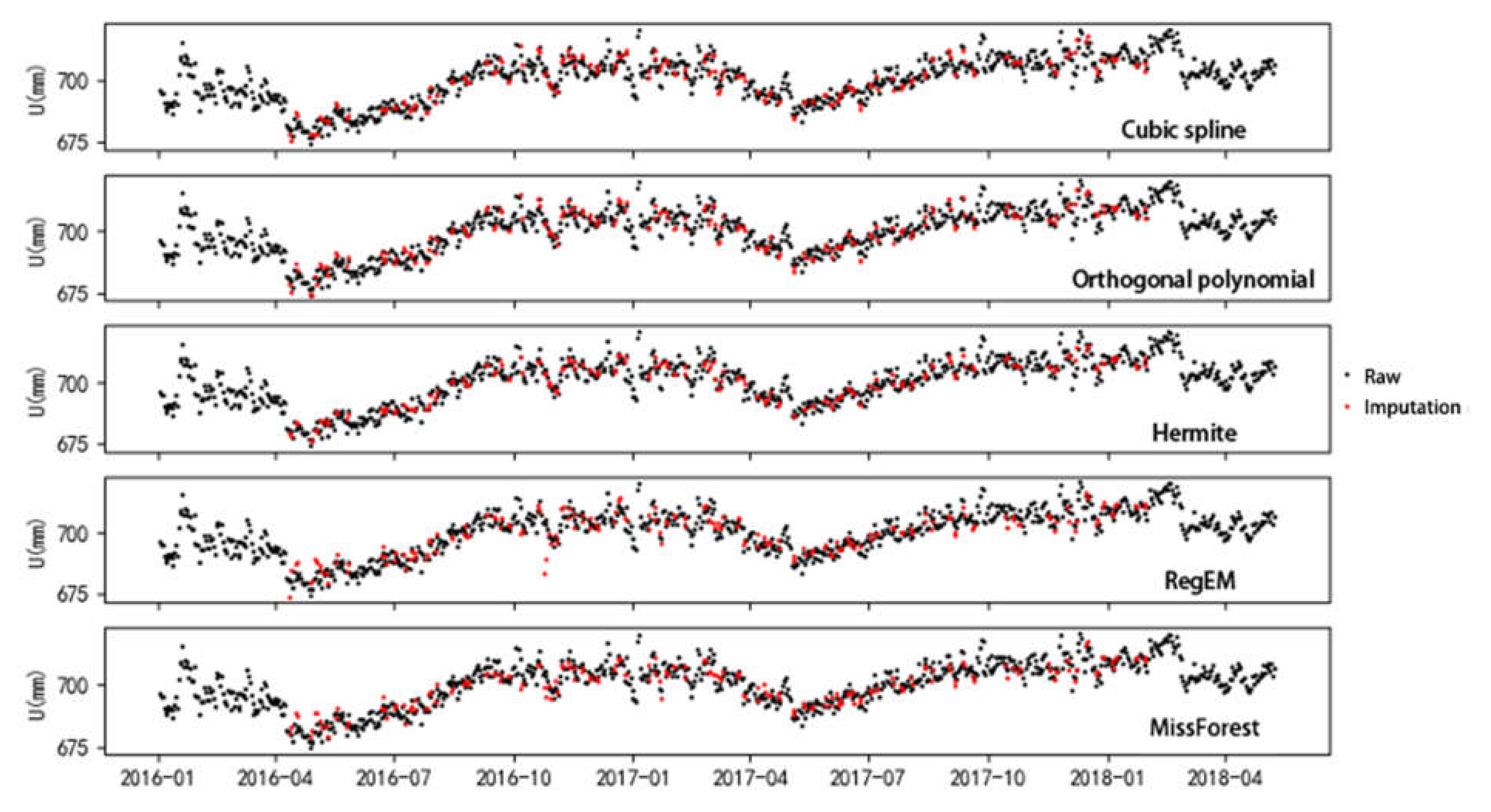
For the imputation results of the 90 by 2-day gap data of the different methods, one trial of the 200 imputation results is shown in Figure 4. MAE, NRMSE, and the correlation coefficient (Rp) are shown in Table 1. No obvious difference is observed among the different imputation methods in Figure 4, and only RegEM imputation shows anomalous results in 2016/11. This anomaly is due to a large fluctuation in 2016/11, and RegEM cannot impute this large fluctuation well. missForest can impute the fluctuation well due to its strong modeling capability. Figure 4 and Table 1 indicate that the correlation coefficients of each method are high with a 2-day gap. The Rp, MAE, and NRMSE of missForest are 0.93, 2.55 mm, and 0.062, respectively. The cubic spline has an Rp of 0.68, but those of the others are all above 0.85. The MAE values of the temporal methods range from 3.02 to 5.00, and the cubic spline is about twice the values of missForest. In the case of a small gap size, the temporal relationship methods are not worse than the spatial methods (RegEM and missForest) because the missing points have a strong relationship with their adjacent observations.
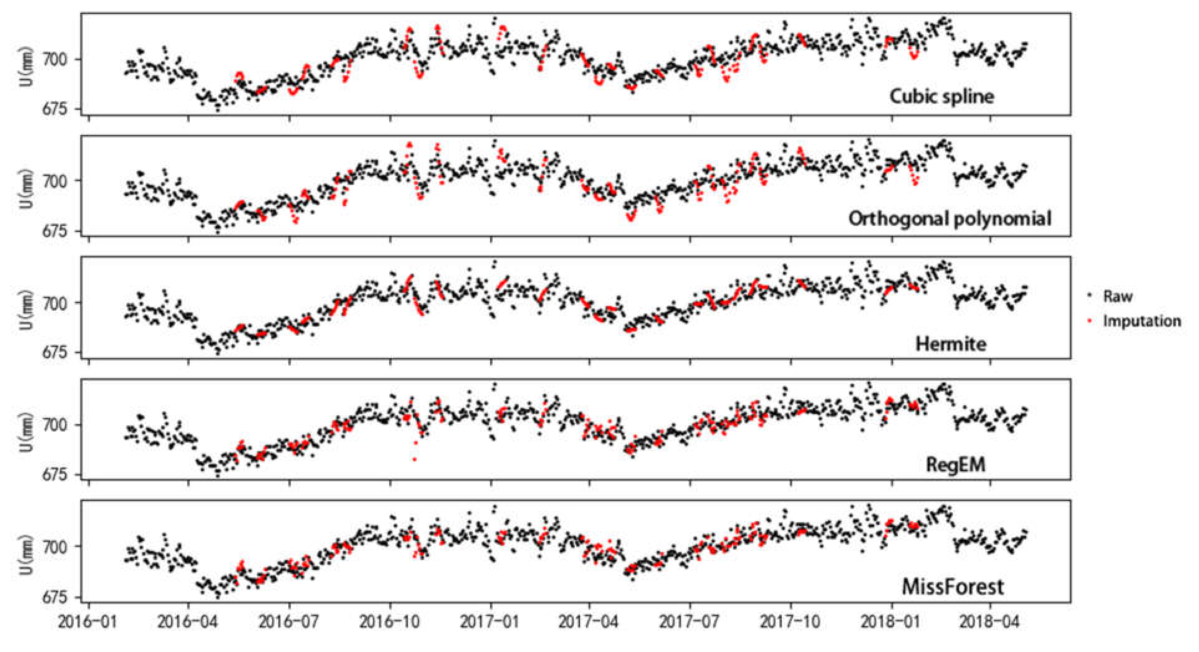
3.1.2. 7-Day Gap
For the imputation results of the 20 by 7-day gap data of the different methods, one trial of the imputation results is shown in Figure 5. Cubic spline and orthogonal polynomial show large fluctuations in Figure 5 because these methods become unstable when the gap size increases. As shown in Table 1, the MAE of orthogonal polynomial increases from 3.67 to 6.27 mm and is worse than that of cubic spline, which means that this method is unstable for large gaps. The Rp and NRMSE of missForest are 0.92 and 0.063, respectively, and the MAE of missForest is 2.61 mm, which is increased by only 0.06 mm. The smallest degradation of missForest among all the methods means that missForest is more stable than the others. missForest uses the bootstrap approach to sample the dataset and generate many regression trees to derive the missing value. This procedure prevents any poor regression tree from affecting the overall results.
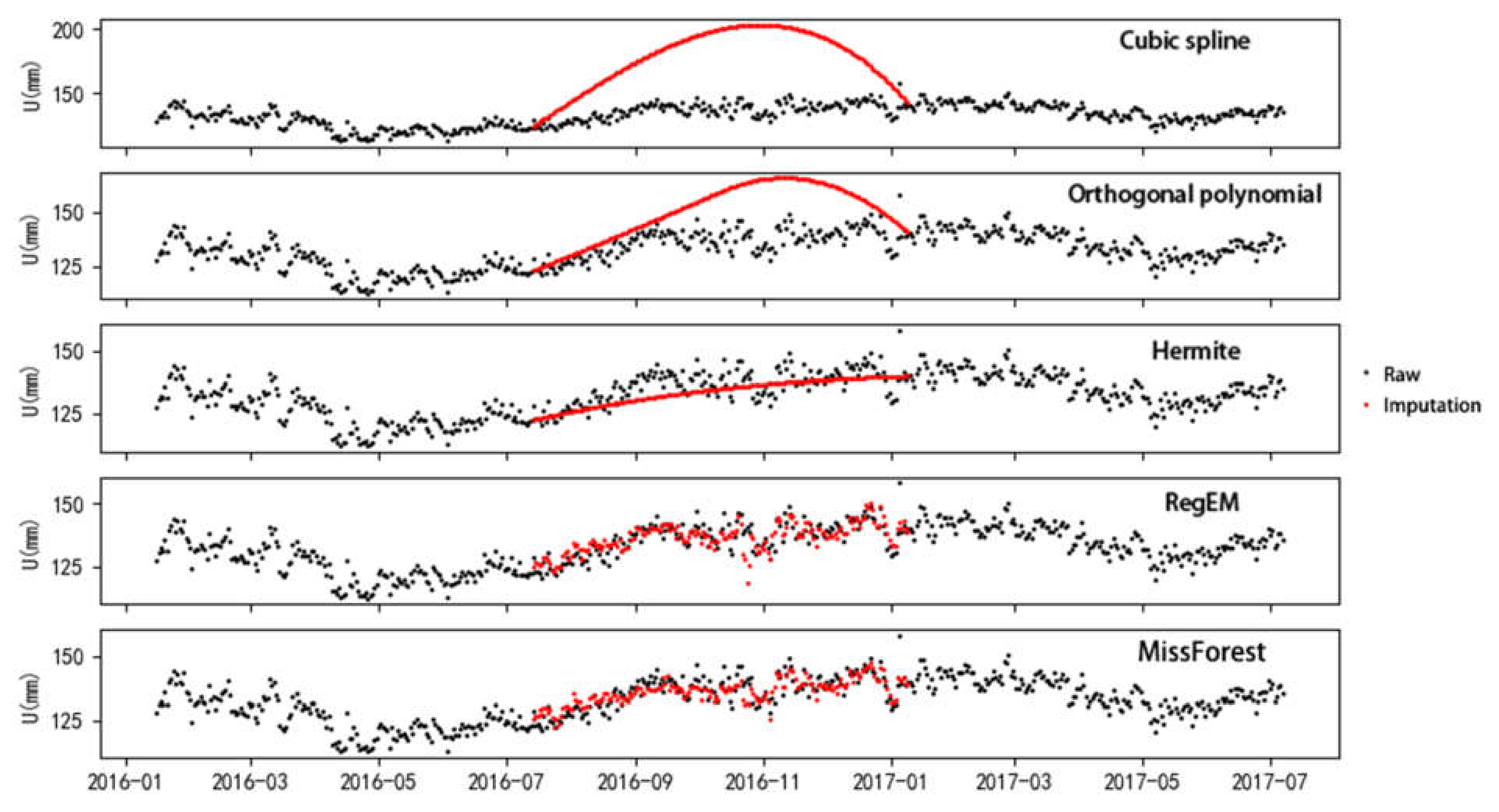
3.1.3. 30-Day Gap
For the imputation results of the 6 by 30-day gap data of the different methods, one trial of the imputation results is shown in Figure 6. The results of cubic spline and orthogonal polynomial in Figure 6 have large biases from the true value, and the MAE of the orthogonal polynomial in Table 1 is larger than 19 mm. The Hermite methods produce over-smooth results with respect to the other methods because Hermite requires the values of functions on nodes and the values of corresponding derivatives (even those of higher derivatives) to be equal. The correlation coefficient of the orthogonal polynomial is below 0.7. The Rp, MAE, and NRMSE of missForest are 0.92, 2.71 mm, and 0.065, respectively. The results of the methods using temporal correlation are smoother than those of the methods using spatial correlation, and the MAE and NRMSE of RegEM and missForest are smaller than those of the others. The methods that use temporal correlation cannot react to complicated time variations, obtain poor results with a large gap size, and may result in artificial signals.
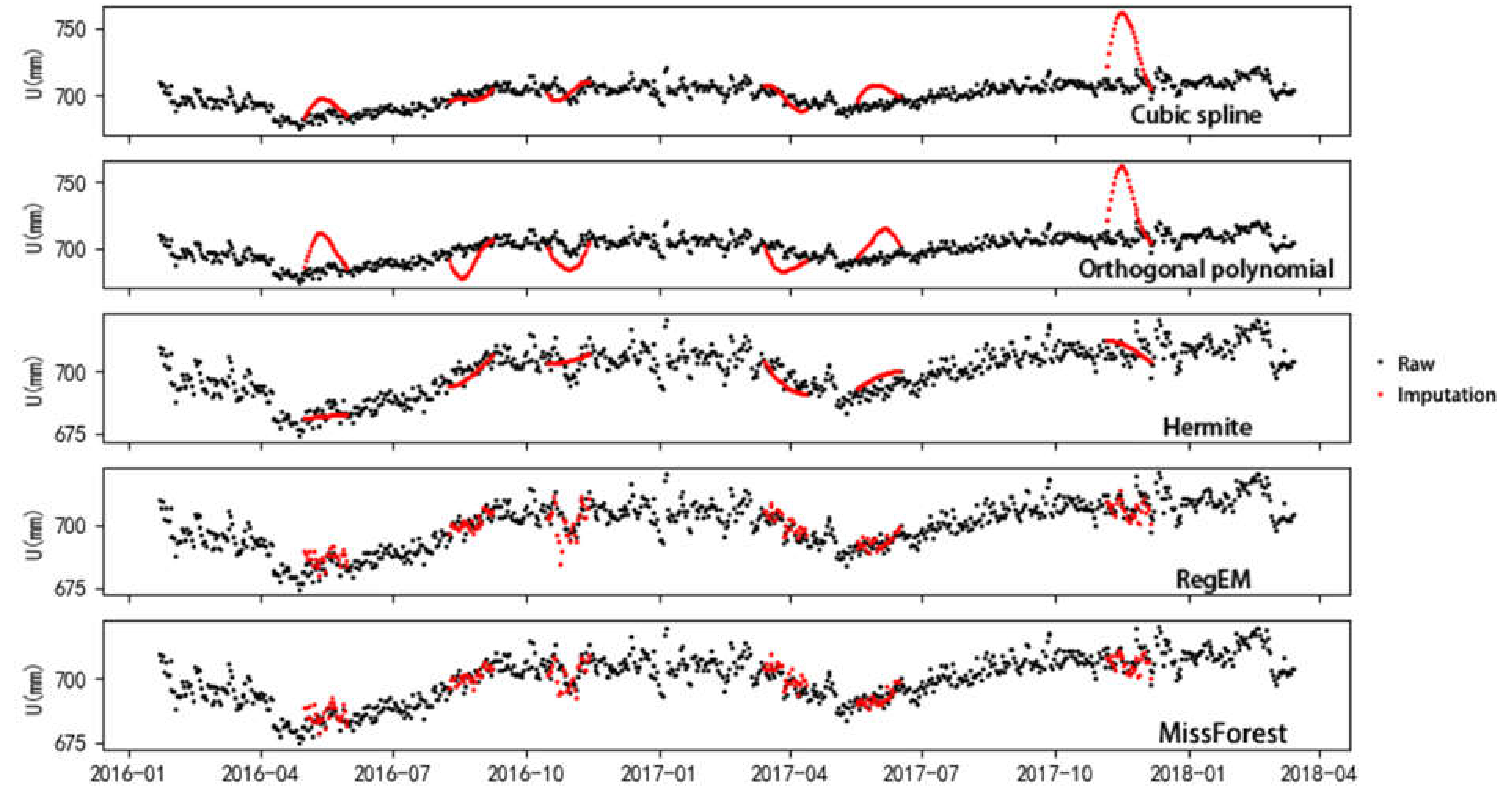
3.1.4. 180-Day Gap
For the imputation results of the 180-day gap data of the different methods, one trial of the imputation results is shown in Figure 7. The results of cubic spline and orthogonal polynomial in Figure 7 show large deviations. Hermite only fits a major linear trend and loses many details. As indicated in Table 1, missForest has a strong linear correlation. The Rp of missForest and RegEM is 0.90 and 0.83, respectively. The MAE and NRMSE of missForest are 2.95 mm and 0.066, respectively, which are about half of the values of Hermite and cubic spline. Figure 4, Figure 5, Figure 6 and Figure 7 show that cubic spline and orthogonal polynomial are only suitable for small gap sizes. Comparison of the results of RegEM and missForest indicates that RegEM has several outliers (Figure 7), but no obvious outliers are found in the missForest method. The results of missForest outperform those of RegEM, indicating that missForest can restore more information from data than RegEM can. Moreover, the dataset (GPS coordinate time series) contains several nonlinear relationships that only missForest can restore because missForest can consider nonlinear relationships, whereas RegEM only considers linear relationships.
3.2. Different Missing Rate Analysis
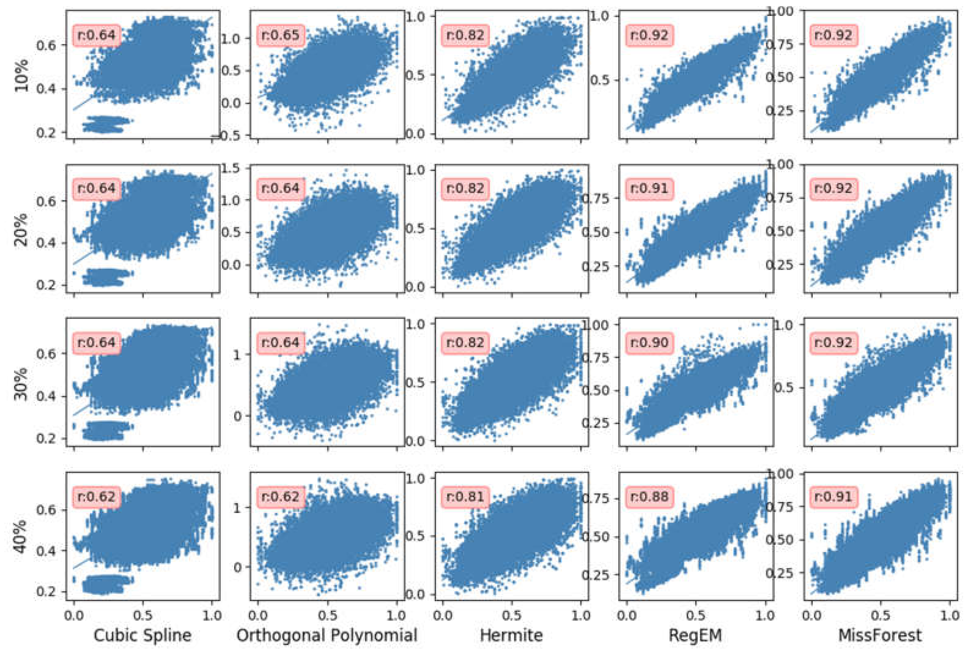
To understand the performance of the various methods under different missing rates, we randomly remove 10%, 20%, 30%, and 40% data at 10 random stations with a 7-day gap as a gappy time series to perform the following analysis. We also conduct 200 random trials and average the MAE, NRMSE, and Rp of all trials (Figure 8 and Table 2). Among all the results of different methods for different missing rates shown in Figure 8 and Table 2, those of missForest are the best. The imputation results of different methods have different distribution characteristics, as shown in Figure 8. The traditional method is divergent, and missForest has the best correlation relationship. When the missing rate is 10%, the results of cubic spline and orthogonal polynomial are the worst; the MAE and NRMSE values of RegEM and missForest are about half of the values for cubic spline and orthogonal polynomial. When the missing rate increases to 20%, the MAE and Rp of the temporal methods change slightly because cubic spline and orthogonal polynomial focus on local time correlation, and MAE changes only slightly. When the missing rate increases to 30%, the MAE of RegEM increases from 2.82 to 3.12, whereas the MAE of missForest only changes from 2.66 to 2.68. The change for RegEM is larger than that for missForest. When the missing rate increases to 40%, the RP, MAE, and NRMSE of missForest are 0.91, 2.74 mm, and 0.064, respectively, and those of RegEM are 0.88, 3.48 mm, and 0.081, respectively. This result indicates that when the number of observations is small, missForest can obtain more information and produce better imputation results than RegEM. The temporal methods only use the before and after observations at the time of the gap, whereas RegEM and missForest can take information from other stations at the missing time. Comparison of RegEM and missForest indicates that missForest has slightly better imputation results because it considers nonlinear relationships and can therefore restore more information and improve the imputation performance.
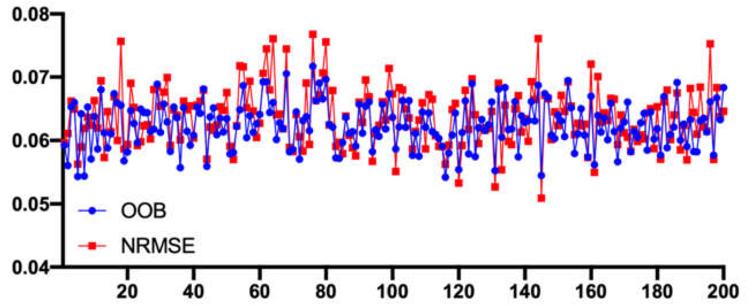
3.3. OOB versus NRMSE
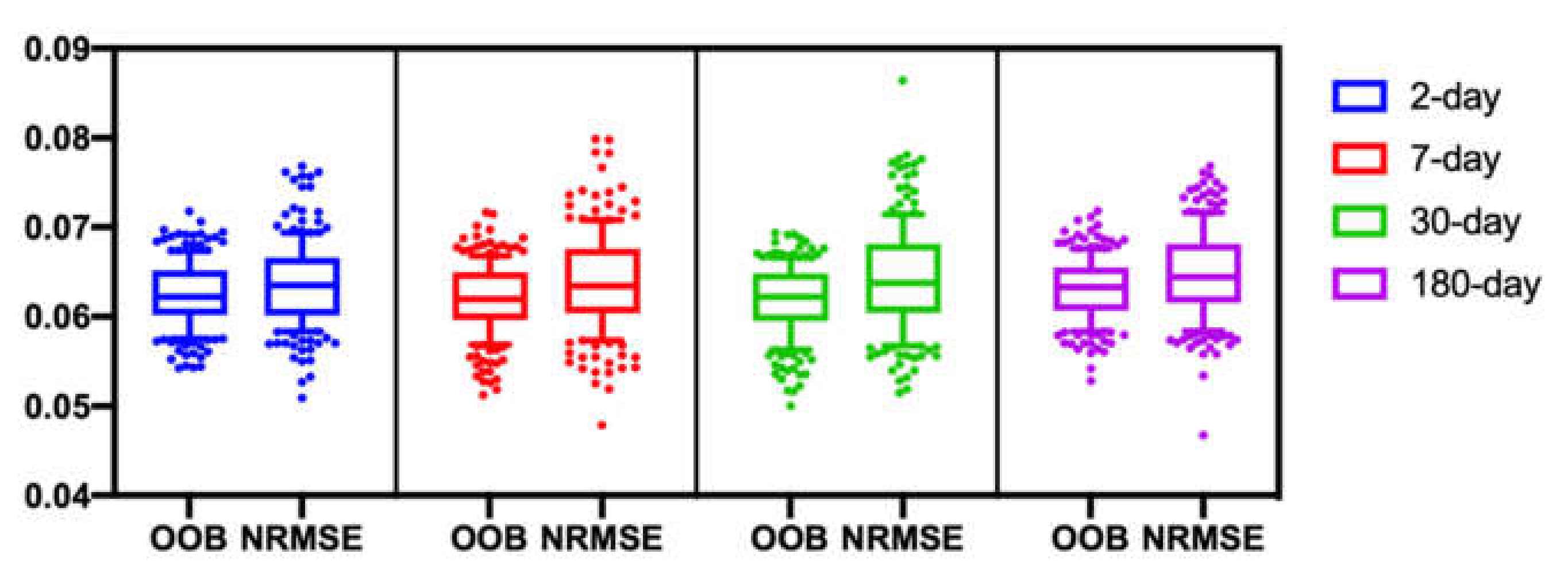
To compare the distance between OOB and NRMSE, we calculate the OOB and NRMSE of 200 trials with a gap rate of 20% and gap size of 2-day, 7-day, 30-day, and 180-day. Figure 9 shows 2-day gap size results and we can see that OOB and NRMSE are close, although OOB is a little smaller than NRMSE, which is usually caused by overfitting. The Pearson correlation coefficient of OOB and NMSE is 0.74. Figure 10 shows all results of 2-day, 7-day, 30-day, and 180-day, and we can see the OOB estimates exhibit a lot less variability than NRMSE in all gap sizes. The OOB estimates tend to slightly underestimate the imputation error with all gap sizes. However, on average, the estimation is comparably good. This result indicates that we can use OOB as the approximate value of the real NRMSE.
3.4. PCA of Different Gap Sizes
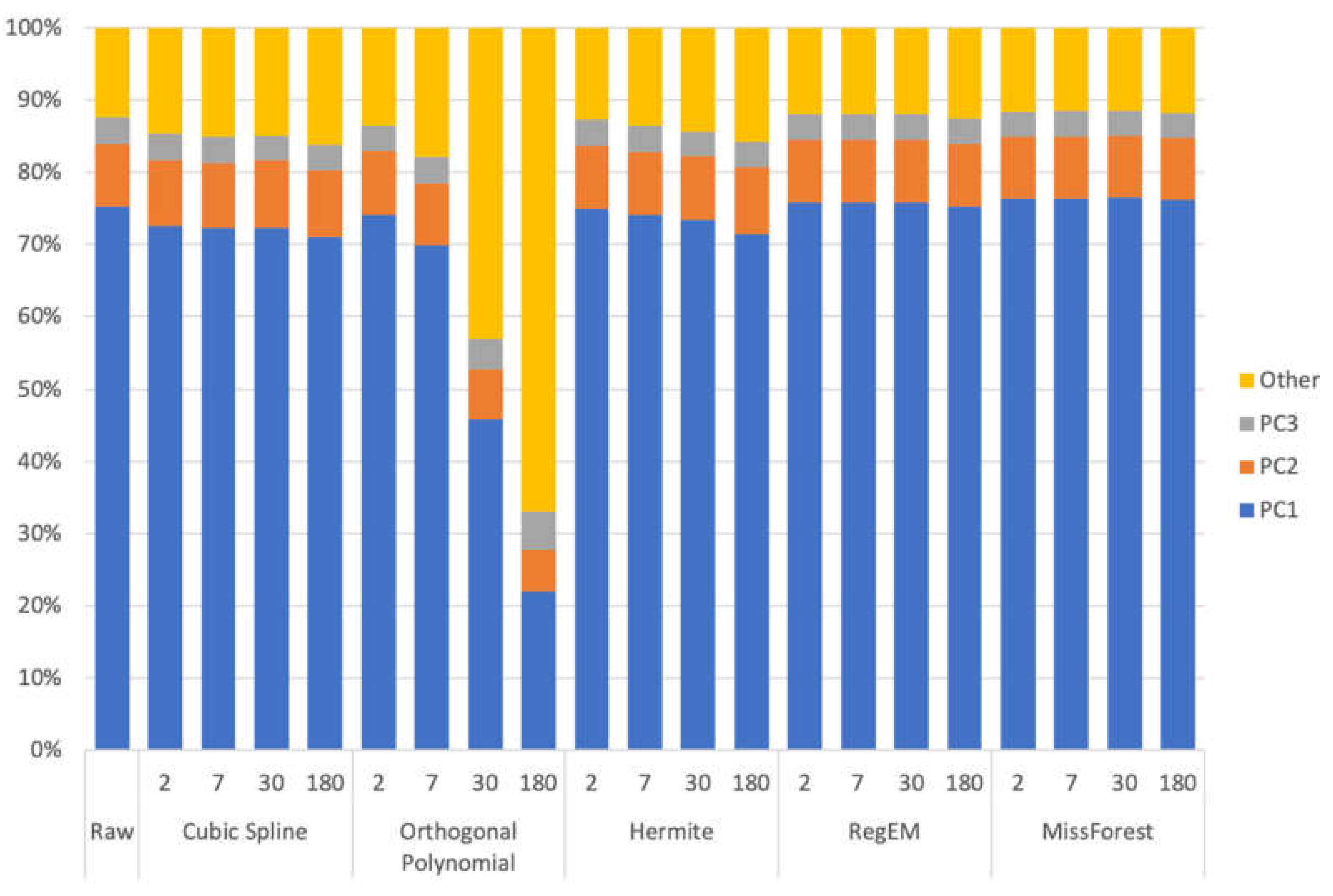
To determine the influence of different methods on PCA, we use the results of 200 trials and perform PCA on them. We compute the proportion of the variance of the first three PCs and the distance and angle of PC1 between the original data and imputed data (Table 3 and Figure 11). Figure 11 shows that the two best methods are RegEM and missForest. The other methods somewhat change the proportion of PCs. As the gap size increases, the difference between imputed and original data becomes increasingly obvious (especially for the orthogonal polynomial method) because of the instability of the temporal methods with gap size. When the gap size is 2 days, the distance of RegEM and missForest are 0.008 and 0.009, respectively (Table 3). Cubic spline and Hermite have 0.049 and 0.023, respectively, which are several times larger than those of RegEM and missForest. The angle of the results from cubic spline is the largest, whereas that from RegEM is the smallest. When the gap size increases to 7 days, the orthogonal polynomial method changes considerably. When the gap size increases to 30 days, the distance of orthogonal polynomial changes to 0.341, which is smaller than that of cubic spline, but the angle of orthogonal polynomial is 19.707, whereas that of cubic spline is 2.790. This result indicates that only distance and angle can reflect the real difference. When the gap size is 180 days, the distance of missForest is 0.024, and the angle is 1.408; both are the smallest among all the values for the compared methods. Hence, missForest can better restore the information in the time series and is more robust than the other methods using time correlation. In other words, missForest can restore abundant information from existing data, and imputed data from missForest are suitable and reliable to use in PCA.
3.5. Time Consumption
The time consumption does not change too much with the gap size and gap rate. We compared the average time of 200 trials. We evaluate the time consumption of our algorithm and the baseline methods on a desktop PC (with i5-9600k). As shown in Table 4, the orthogonal polynomial and Hermite run fastest, and the missForest is slower than other methods because of the usage of many random forests. missForest’s time consumption (5.58 s) in the GPS time series process is tolerable with the 20 GPS station time series of 2016-2018 in Greenland to process.
4. Discussion and Conclusions
In this study, GPS time series from January 2016 to June 2018 in Greenland were processed using different imputation methods. The performance of five methods was assessed, and the methods’ impact on PCA was investigated by comparing the change in principal components. The NRMSE and MAE of missForest were the best overall. When the gap size increased from 2 days to 180 days, the MAE of missForest changed by only 0.4 mm. This result means that missForest can perform well regardless of the gap size. It can simplify our process of GPS time series because in traditional methods, we need to use different methods/assumptions to impute missing values for different gap sizes.
To investigate the impact of different imputation methods on the signals in GPS time series, we used PCA to assess the results of the different imputation methods. We computed the proportion of the variance of the first three principal components after imputation. The results showed that the traditional methods changed the proportion to some extent and their performance worsened as the gap size increased. RegEM and missForest obtained stable and reliable imputation results relative to the original (true) data. To further investigate the variations caused by different imputation methods on the principal components, we computed the distance and angle of PC1 between the original and imputed data. The result of missForest was the best. This method is beneficial to the subsequent analysis of GPS time series.
Traditional methods only use the temporal correlation in the data, and their results worsen as the gap size increases. Inspired by RegEM, we utilized the spatial correlation between time series and a machine learning method (missForest) to restore abundant information in the imputation. By using spatial correlation, we can use observations from other stations to impute the missing stations while restoring the missing information as much as possible and avoiding the introduction of artificial information, such as in temporal methods. From the statistical results of different missing rates for the different methods, we can conclude that considering the spatial relationship produces more reliable and robust imputation results than considering only the temporal relationship. The main results of this study are as follows; (1) missForest can fill more than a 7-day gap with high accuracy, (2) missForest can fill data with a high gap rate or few samples, (3) missForest can effectively restore the information in time series. Overall, the MAE and NRMSE of missForest are only half of those of traditional methods. The MAE and NRMSE of missForest show a 12% improvement compared with the values for RegEM. Obtaining accurate imputed data can improve the results of related processes, such as PCA.
Author Contributions
Conceptualization, S.Z.; validation, F.X., Q.Z. and W.L.; formal analysis, L.G. and J.L.; writing—original draft preparation, S.Z. and L.G.; writing—review and editing, S.Z. and J.L.; supervision, S.Z. and J.L.; funding acquisition, S.Z. and W.L.; All authors have read and agreed to the published version of the manuscript.
Funding
This research was funded by the National Key Research and Development Program of China, grant number 2017YFA0603104 and the State Key Program of National Natural Science Foundation of China, grant number 42074006.
Data Availability Statement
The GPS time series data used in this paper can be freely accessed at http://geodesy.unr.edu/NGLStationPages/GlobalStationList .
Acknowledgments
The numerical calculations in this study were conducted in the Supercomputing Center of Wuhan University. We acknowledge the Nevada Geodetic Laboratory for providing the GPS time series used in this study. We thank editors and four anonymous reviewers for providing constructive comments, which have improved this manuscript.
Conflicts of Interest
The authors declare no conflict of interest.
References
- Liu, N.; Dai, W.; Santerre, R.; Kuang, C. A MATLAB-Based Kriged Kalman Filter Software for Interpolating Missing Data in GNSS Coordinate Time Series. GPS Solut. 2017, 22, 25. [Google Scholar] [CrossRef]
- Shirzaei, M.; Bürgmann, R.; Foster, J.; Walter, T.R.; Brooks, B.A. Aseismic Deformation across the Hilina Fault System, Hawaii, Revealed by Wavelet Analysis of InSAR and GPS Time Series. Earth Planet. Sci. Lett. 2013, 376, 12–19. [Google Scholar] [CrossRef]
- Liu, B.; King, M.; Dai, W. Common Mode Error in Antarctic GPS Coordinate Time-Series on Its Effect on Bedrock-Uplift Estimates. Geophys. J. Int. 2018, 214, 1652–1664. [Google Scholar] [CrossRef]
- Dong, D.; Fang, P.; Bock, Y.; Webb, F.; Prawirodirdjo, L.; Kedar, S.; Jamason, P. Spatiotemporal Filtering Using Principal Component Analysis and Karhunen-Loeve Expansion Approaches for Regional GPS Network Analysis. J. Geophys. Res. Solid Earth 2006, 111. [Google Scholar] [CrossRef] [Green Version]
- He, X.; Hua, X.; Yu, K.; Xuan, W.; Lu, T.; Zhang, W.; Chen, X. Accuracy Enhancement of GPS Time Series Using Principal Component Analysis and Block Spatial Filtering. Adv. Space Res. 2015, 55, 1316–1327. [Google Scholar] [CrossRef]
- Chen, Q.; Van Dam, T.; Sneeuw, N.; Collilieux, X.; Weigelt, M.; Rebischung, P. Singular Spectrum Analysis for Modeling Seasonal Signals from GPS Time Series. J. Geodyn. 2013, 72, 25–35. [Google Scholar] [CrossRef]
- Donders, A.R.T.; Van der Heijden, G.J.M.G.; Stijnen, T.; Moons, K.G.M. Review: A Gentle Introduction to Imputation of Missing Values. J. Clin. Epidemiol. 2006, 59, 1087–1091. [Google Scholar] [CrossRef] [PubMed]
- Robinson, A.P.; Hamann, J.D. Forest Analytics with R: An Introduction; Springer Science & Business Media: Berlin/Heidelberg, Germany, 2010. [Google Scholar]
- Xu, C. Reconstruction of Gappy GPS Coordinate Time Series Using Empirical Orthogonal Functions. J. Geophys. Res. Solid Earth 2016, 121, 9020–9033. [Google Scholar] [CrossRef]
- Wang, X.; Cheng, Y.; Wu, S.; Zhang, K. An Effective Toolkit for the Interpolation and Gross Error Detection of GPS Time Series. Surv. Rev. 2016, 48, 202–211. [Google Scholar] [CrossRef]
- Schneider, T. Analysis of Incomplete Climate Data: Estimation of Mean Values and Covariance Matrices and Imputation of Missing Values. J. Clim. 2001, 14, 20. [Google Scholar] [CrossRef]
- Li, W.; Li, F.; Zhang, S.; Lei, J.; Zhang, Q.; Yuan, L. Spatiotemporal Filtering and Noise Analysis for Regional GNSS Network in Antarctica Using Independent Component Analysis. Remote. Sens. 2019, 11, 386. [Google Scholar] [CrossRef] [Green Version]
- Van Buuren, S.; Oudshoorn, K. Flexible Multivariate Imputation by MICE; TNO: Leiden, The Netherlands, 1999. [Google Scholar]
- Little, R.J.A.; Rubin, D.B. Bayes and Multiple Imputation. In Statistical Analysis with Missing Data; John Wiley & Sons, Ltd.: Hoboken, NJ, USA, 2002; pp. 200–220. ISBN 978-1-119-01356-3. [Google Scholar]
- Barnard, J.; Rubin, D.B. Small-Sample Degrees of Freedom with Multiple Imputation. Biometrika 1999, 86, 948–955. [Google Scholar] [CrossRef]
- Blewitt, G.; Lavallée, D. Effect of Annual Signals on Geodetic Velocity. J. Geophys. Res. Solid Earth 2002, 107, ETG 9-1–ETG 9-11. [Google Scholar] [CrossRef] [Green Version]
- Forsyth, D.A.; Ponce, J. Computer Vision: A Modern Approach, 2nd Ed. ed; Pearson: London, UK, 2012; ISBN 978-0-13-608592-8. [Google Scholar]
- Szeliski, R. Computer Vision: Algorithms and Applications; Springer Science & Business Media: Berlin/Heidelberg, Germany, 2010. [Google Scholar]
- Chowdhury, G.G. Natural Language Processing. Annu. Rev. Inf. Sci. Technol. 2003, 37, 51–89. [Google Scholar] [CrossRef] [Green Version]
- Indurkhya, N.; Damerau, F.J. Handbook of Natural Language Processing; CRC Press: Boca Raton, FL, USA, 2010; Volume 2. [Google Scholar]
- Cao, W.; Wang, D.; Li, J.; Zhou, H.; Li, L.; Li, Y. BRITS: Bidirectional Recurrent Imputation for Time Series. In Advances in Neural Information Processing Systems 31; Bengio, S., Wallach, H., Larochelle, H., Grauman, K., Cesa-Bianchi, N., Garnett, R., Eds.; Curran Associates, Inc.: Red Hook, NY, USA, 2018; pp. 6775–6785. [Google Scholar]
- Yoon, J.; Jordon, J.; Van der Schaar, M. GAIN: Missing Data Imputation Using Generative Adversarial Nets. In Proceedings of the 35th International Conference on Machine Learning, PLMR, Stockholm Sweden, 10–15 July 2018; 2018; 80, pp. 5689–5698. [Google Scholar]
- Stekhoven, D.J.; Buhlmann, P. missForest--Non-Parametric Missing Value Imputation for Mixed-Type Data. Bioinformatics 2012, 28, 112–118. [Google Scholar] [CrossRef] [PubMed] [Green Version]
- Waljee, A.K.; Mukherjee, A.; Singal, A.G.; Zhang, Y.; Warren, J.; Balis, U.; Marrero, J.; Zhu, J.; Higgins, P.D. Comparison of Imputation Methods for Missing Laboratory Data in Medicine. BMJ Open 2013, 3. [Google Scholar] [CrossRef] [PubMed]
- Shah, A.D.; Bartlett, J.W.; Carpenter, J.; Nicholas, O.; Hemingway, H. Comparison of Random Forest and Parametric Imputation Models for Imputing Missing Data Using MICE: A CALIBER Study. Am. J. Epidemiol. 2014, 179, 764–774. [Google Scholar] [CrossRef] [PubMed] [Green Version]
- Dyer, S.A.; Dyer, J.S. Cubic-Spline Interpolation. IEEE Instrum. Meas. Mag. 2001, 4, 44–46. [Google Scholar] [CrossRef]
- Smith, F.J. An Algorithm for Summing Orthogonal Polynomial Series and Their Derivatives with Applications to Curve-Fitting and Interpolation. Math. Comput. 1965, 19, 33–36. [Google Scholar] [CrossRef]
- Farouki, R.T.; Neff, C.A. Hermite Interpolation by Pythagorean Hodograph Quintics. Math. Comp. 1995, 64, 1589–1609. [Google Scholar] [CrossRef]
- Abdi, H.; Williams, L.J. Principal Component Analysis. Wiley Interdiscip. Rev. Comput. Stat. 2010, 2, 433–459. [Google Scholar] [CrossRef]
- James, G.; Witten, D.; Hastie, T.; Tibshirani, R. An Introduction to Statistical Learning; Springer Texts in Statistics; Springer: New York, NY, USA, 2013; Volume 103, ISBN 978-1-4614-7137-0. [Google Scholar]
- Janitza, S.; Hornung, R. On the Overestimation of Random Forest’s out-of-Bag Error. PLoS ONE 2018, 13, e0201904. [Google Scholar] [CrossRef] [PubMed]
- Blewitt, G.; Hammond, W.C.; Kreemer, C. Harnessing the GPS Data Explosion for Interdisciplinary Science. Eos 2018, 99, 1–2. [Google Scholar] [CrossRef]
Figure 1.
Four parts of X divided by .

Figure 2.
(A) Distribution of GPS stations. (B) Observation epoch of the stations.

Figure 3.
Comparisons of the imputed and true values for different gaps and methods for 200 trials together. The x-axis is true values, and the y-axis is the imputation values (normalized to (0–1) for clarity).
Figure 3.
Comparisons of the imputed and true values for different gaps and methods for 200 trials together. The x-axis is true values, and the y-axis is the imputation values (normalized to (0–1) for clarity).

Figure 4.
Imputation results of 90 by 2-day gap GPS coordinate time series. The y-axis is denormalized to real scale (in mm).
Figure 4.
Imputation results of 90 by 2-day gap GPS coordinate time series. The y-axis is denormalized to real scale (in mm).

Figure 5.
Imputation results of 20 by 7-day gap GPS coordinate time series. The y-aixs is denormalized to real scale (in mm).
Figure 5.
Imputation results of 20 by 7-day gap GPS coordinate time series. The y-aixs is denormalized to real scale (in mm).

Figure 6.
Imputation results of 6 by 30-day gap GPS coordinate time series. The y-aixs is denormalized to real scale (in mm).
Figure 6.
Imputation results of 6 by 30-day gap GPS coordinate time series. The y-aixs is denormalized to real scale (in mm).

Figure 7.
Imputation results of 180-day gap GPS coordinate time series. The y-aixs is denormalized to real scale (in mm).
Figure 7.
Imputation results of 180-day gap GPS coordinate time series. The y-aixs is denormalized to real scale (in mm).

Figure 8.
Comparison of imputed and true values with different missing rates and methods for 200 trials together. The x-axis is true values, and the y-axis is the imputation values (normalized to [0–1] for clarity).
Figure 8.
Comparison of imputed and true values with different missing rates and methods for 200 trials together. The x-axis is true values, and the y-axis is the imputation values (normalized to [0–1] for clarity).

Figure 9.
OOB and NMSE of 200 trials with 2-day gap size.

Figure 10.
2-day, 7-day, 30-day and 180-day gap size OOB–NRMSE comparison of 200 trials.

Figure 11.
Proportion of the variance of the first three principal components after imputation.


Table 1.
MAE, NRMSE, and Pearson coefficient (Rp) of different imputation methods with 90 by 2-day, 20 by 7-day, 6 by 30-day, and 1 by 180-day gaps of GPS time series caption.
Table 1.
MAE, NRMSE, and Pearson coefficient (Rp) of different imputation methods with 90 by 2-day, 20 by 7-day, 6 by 30-day, and 1 by 180-day gaps of GPS time series caption.
| Method | Evaluation | 90 * 2-Day | 20 * 7-Day | 6 * 30-Day | 1 * 180-Day |
|---|---|---|---|---|---|
| Cubic spline | MAE (mm) | 5.00 | 5.10 | 5.31 | 6.18 |
| NRMSE | 0.115 | 0.116 | 0.121 | 0.141 | |
| Rp | 0.68 | 0.67 | 0.68 | 0.42 | |
| Orthogonal polynomial | MAE (mm) | 3.67 | 6.27 | 19.08 | 99.88 |
| NRMSE | 0.088 | 0.152 | 0.471 | 2.509 | |
| Rp | 0.85 | 0.64 | 0.30 | 0.11 | |
| Hermite | MAE (mm) | 3.02 | 3.68 | 4.47 | 5.63 |
| NRMSE | 0.072 | 0.088 | 0.106 | 0.129 | |
| Rp | 0.89 | 0.83 | 0.79 | 0.61 | |
| RegEM | MAE (mm) | 2.81 | 2.84 | 2.96 | 3.40 |
| NRMSE | 0.065 | 0.066 | 0.068 | 0.074 | |
| Rp | 0.92 | 0.91 | 0.91 | 0.83 | |
| missForest | MAE (mm) | 2.55 | 2.61 | 2.71 | 2.95 |
| NRMSE | 0.062 | 0.063 | 0.065 | 0.066 | |
| Rp | 0.93 | 0.92 | 0.92 | 0.90 |
Table 2.
MAE, NRMSE, and Rp of different imputation methods with 10%, 20%, 30% and 40% missing rates of GPS time series.
Table 2.
MAE, NRMSE, and Rp of different imputation methods with 10%, 20%, 30% and 40% missing rates of GPS time series.
| Method | Evaluation | 10% | 20% | 30% | 40% |
|---|---|---|---|---|---|
| Cubic spline | MAE (mm) | 5.48 | 5.52 | 5.53 | 5.58 |
| NRMSE | 0.126 | 0.128 | 0.129 | 0.130 | |
| Rp | 0.64 | 0.64 | 0.64 | 0.62 | |
| Orthogonal polynomial | MAE (mm) | 6.89 | 6.89 | 6.92 | 7.04 |
| NRMSE | 0.161 | 0.161 | 0.162 | 0.165 | |
| Rp | 0.65 | 0.64 | 0.64 | 0.62 | |
| Hermite | MAE (mm) | 3.71 | 3.82 | 4.02 | 4.17 |
| NRMSE | 0.093 | 0.093 | 0.095 | 0.098 | |
| Rp | 0.82 | 0.82 | 0.82 | 0.81 | |
| RegEM | MAE (mm) | 2.76 | 2.82 | 3.12 | 3.48 |
| NRMSE | 0.065 | 0.066 | 0.073 | 0.081 | |
| Rp | 0.92 | 0.91 | 0.90 | 0.88 | |
| missForest | MAE (mm) | 2.64 | 2.66 | 2.68 | 2.74 |
| NRMSE | 0.061 | 0.062 | 0.063 | 0.064 | |
| Rp | 0.92 | 0.92 | 0.92 | 0.91 |
Table 3.
Results of PCA of different methods with multiple gap sizes.
| Method | Gap Size | PC1 (%) | PC2 (%) | PC3 (%) | SUM (%) | Ddistance | Aangle |
|---|---|---|---|---|---|---|---|
| Original | - | 75.24 | 8.73 | 3.57 | 87.55 | 0 | 0 |
| Cubic spline | 2 | 72.53 | 9.17 | 3.63 | 85.35 | 0.049 | 2.828 |
| 7 | 72.22 | 9.09 | 3.56 | 84.88 | 0.050 | 2.890 | |
| 30 | 72.32 | 9.41 | 3.38 | 85.12 | 0.048 | 2.790 | |
| 180 | 71.05 | 9.28 | 3.51 | 83.85 | 0.057 | 3.26 | |
| Orthogonal polynomial | 2 | 74.17 | 8.76 | 3.58 | 86.52 | 0.009 | 0.555 |
| 7 | 69.87 | 8.55 | 3.72 | 82.15 | 0.318 | 1.823 | |
| 30 | 45.89 | 6.86 | 4.25 | 57.02 | 0.341 | 19.707 | |
| 180 | 22.00 | 5.69 | 5.41 | 33.10 | 1.041 | 63.12 | |
| Hermite | 2 | 74.89 | 8.81 | 3.56 | 87.27 | 0.023 | 1.374 |
| 7 | 74.11 | 8.77 | 3.60 | 86.49 | 0.026 | 1.494 | |
| 30 | 73.37 | 8.87 | 3.41 | 85.66 | 0.029 | 1.668 | |
| 180 | 71.48 | 9.26 | 3.53 | 84.29 | 0.050 | 2.881 | |
| RegEM | 2 | 75.86 | 8.65 | 3.54 | 88.06 | 0.008 | 0.501 |
| 7 | 75.79 | 8.69 | 3.51 | 88.00 | 0.015 | 0.859 | |
| 30 | 75.83 | 8.73 | 3.44 | 88.01 | 0.027 | 1.572 | |
| 180 | 75.27 | 8.69 | 3.57 | 87.53 | 0.037 | 2.121 | |
| missForest | 2 | 76.36 | 8.59 | 3.43 | 88.38 | 0.009 | 0.572 |
| 7 | 76.38 | 8.61 | 3.41 | 88.41 | 0.010 | 0.619 | |
| 30 | 76.45 | 8.68 | 3.31 | 88.45 | 0.013 | 0.764 | |
| 180 | 76.23 | 8.55 | 3.45 | 88.24 | 0.024 | 1.408 |
Table 4.
The time consumption for all imputation methods.
| METHOD | Cubic Spline | Orthogonal Polynomial | Hermite | RegEM | missForest |
|---|---|---|---|---|---|
| Time (s) | 0.14 | 0.10 | 0.09 | 0.48 | 5.58 |
Publisher’s Note: MDPI stays neutral with regard to jurisdictional claims in published maps and institutional affiliations. |
© 2021 by the authors. Licensee MDPI, Basel, Switzerland. This article is an open access article distributed under the terms and conditions of the Creative Commons Attribution (CC BY) license (https://creativecommons.org/licenses/by/4.0/).
Share and Cite
MDPI and ACS Style
Zhang, S.; Gong, L.; Zeng, Q.; Li, W.; Xiao, F.; Lei, J. Imputation of GPS Coordinate Time Series Using missForest. Remote Sens. 2021, 13, 2312. https://doi.org/10.3390/rs13122312
AMA Style
Zhang S, Gong L, Zeng Q, Li W, Xiao F, Lei J. Imputation of GPS Coordinate Time Series Using missForest. Remote Sensing. 2021; 13(12):2312. https://doi.org/10.3390/rs13122312
Chicago/Turabian StyleZhang, Shengkai, Li Gong, Qi Zeng, Wenhao Li, Feng Xiao, and Jintao Lei. 2021. "Imputation of GPS Coordinate Time Series Using missForest" Remote Sensing 13, no. 12: 2312. https://doi.org/10.3390/rs13122312
Note that from the first issue of 2016, this journal uses article numbers instead of page numbers. See further details here.