
Assessment of Deep Learning Techniques for Land Use Land Cover Classification in Southern New Caledonia


1
ESPACE-DEV, Univ New Caledonia, Univ Montpellier, IRD, Univ Antilles, Univ Guyane, Univ Réunion, 98800 New Caledonia, France
2
ISEA, Univ New Caledonia, 98800 New Caledonia, France
3
Photogrammetry and Remote Sensing, ETH Zurich, 8093 Zurich, Switzerland
4
Institut de Recherche pour le Développement, UMR 9220 ENTROPIE (Institut de Recherche pour le Développement, Université de la Réunion, IFREMER, Université de la Nouvelle-Calédonie, Centre National de la Recherche Scientifique), 98800 New Caledonia, France
*
Author to whom correspondence should be addressed.
Remote Sens. 2021, 13(12), 2257; https://doi.org/10.3390/rs13122257
Submission received: 31 March 2021
/
Revised: 25 May 2021
/
Accepted: 27 May 2021
/
Published: 9 June 2021
Abstract
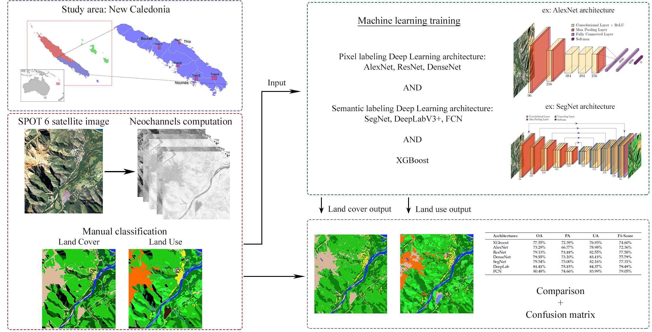
:Land use (LU) and land cover (LC) are two complementary pieces of cartographic information used for urban planning and environmental monitoring. In the context of New Caledonia, a biodiversity hotspot, the availability of up-to-date LULC maps is essential to monitor the impact of extreme events such as cyclones and human activities on the environment. With the democratization of satellite data and the development of high-performance deep learning techniques, it is possible to create these data automatically. This work aims at determining the best current deep learning configuration (pixel-wise vs. semantic labelling architectures, data augmentation, image prepossessing, …), to perform LULC mapping in a complex, subtropical environment. For this purpose, a specific data set based on SPOT6 satellite data was created and made available for the scientific community as an LULC benchmark in a tropical, complex environment using five representative areas of New Caledonia labelled by a human operator: four used as training sets, and the fifth as a test set. Several architectures were trained and the resulting classification was compared with a state-of-the-art machine learning technique: XGboost. We also assessed the relevance of popular neo-channels derived from the raw observations in the context of deep learning. The deep learning approach showed comparable results to XGboost for LC detection and over-performed it on the LU detection task (61.45% vs. 51.56% of overall accuracy). Finally, adding LC classification output of the dedicated deep learning architecture to the raw channels input significantly improved the overall accuracy of the deep learning LU classification task (63.61% of overall accuracy). All the data used in this study are available on line for the remote sensing community and for assessing other LULC detection techniques.

1. Introduction
Maps of Land Use and Land Cover (LULC) are an elementary tool for environmental planning and decision-making. As the name implies, the term comprises two related, but different pieces of information about a geographical location, the land use (LU) according to its function in terms of human use (such as farm, airport, road, etc.), and the land cover (LC) according to the physical/chemical material (such as vegetation, bare soil, etc.). Both LC and LU classes, normally defined in hierarchical schemes, play an important role for planning and management of the natural and built environment at different granularities [1]. A primary data source to generate LULC maps is remotely sensed imagery, which serves as a basis for either photo-interpretation by a human operator, or automated classification with suitable classification algorithms. Remote sensing imagery at different wavelengths of the electromagnetic spectrum has proven effective for environmental monitoring at various spatial and spectral resolutions [2,3]. In particular, recent satellites observe the Earth’s surface with small ground sampling distances (GSD) and high temporal revisit rates [4], which makes them suitable for environmental monitoring of remote territories, where other data sources are difficult to sustain the monitoring.
A case in point is New Caledonia, a biodiversity hotspot [5,6] whose monitoring on a regular, periodic basis is essential for environmental management and conservation. New Caledonia is a tropical high-island with a comparatively small population distributed unevenly across its territory, large areas of dense vegetation, and considerable, intense mining activities that have led to significant erosion phenomena [7]. The resulting complex environment [8,9,10] requires environmental monitoring at a fine scale by the use of very high spatial resolution satellite imagery. The Government of New Caledonia has commissioned the production of an LU map of the entire territory from the New Caledonia Environmental Observatory, using 2014 SPOT6 satellite images [11]. That map, available at medium resolution (minimum mapping unit 0.01 km), is widely used by the country’s decision makers to monitor the environmental impact of mining and the decline of tropical forests over the entire territory. However, the product at present covers only the southern part of New Caledonia. Moreover, its creation, requiring a lot of human input, was time-consuming and costly. No updates are foreseen for several years, for lack of resources. Consequently, there is a need for automation.
Among comparisons of methods to classify LULC from satellite images on several benchmark datasets, Deep Learning has recently stood out as a particularly effective framework for automatic image interpretation [12]. Given large amounts of training data, Deep Learning is able to extract very complex decision rules [13]. In image processing in particular, Deep Learning is at the top of the state-of-the-art semantic image analyses [14] (described in the Methods section), greatly enhanced by the particular design of the convolutional deep networks. Indeed, on some tasks its performance matches or even exceeds that of humans [15]. Additionally in optical satellite remote sensing, Deep Learning has become a standard tool, as it appears to cope particularly well with the continuously varying imaging conditions (illumination, sensor properties, atmospheric composition, etc.) [16,17,18]. Deep Learning has been widely employed for remote sensing, including tasks such as object recognition, scene type recognition or pixel-wise classification [19,20].
In this article, several Deep Learning architectures for LULC classification are compared across five specific regions of South Province of New Caledonia. The goal is to prepare an operational system for LULC monitoring for the South Province territory, since its natural environment is subject to significant human pressures [21,22]. Many powerful Deep Learning architectures in the field of remote sensing use two possible strategies: “central-pixel labeling” or “semantic segmentation” (described in the Methods section).
We empirically compare a number of these promising Deep Learning architectures. Moreover we also include a standard machine learning baseline, XGboost, which has shown very good performances in several benchmarks related to classification [23]. Since “neo-channels”, which are non-linear combinations of the raw channels, and texture filters derived by arithmetic combinations of the raw image channels are widely used in the field of remote sensing [24], we also assess the interest of such additional information when using XGboost and Deep Learning, even if in the latter case, the technique is able to build its own internal features by combining the raw information.
Finally, LU mapping is a considerably harder task than LC mapping. LC mapping is generally obtained by photo-interpretation of satellite and/or aerial images, while LU mapping typically requires the integration of exogenous data (road network map, flood zones, agricultural areas, etc.) and ground surveys due to the difficulty of interpreting satellite images. However, for this study these exogenous data sources are not available and the LU mapping is also created by photo-interpretation. In addition, in this study, the LU nomenclature has a higher number of distinct classes than the LC nomenclature. We construct a two-step architecture and show that LU retrieval can be improved by first classifying LC and then using its class labels as an additional input.
2. Materials
2.1. Study Area: New Caledonia
As part of a project commissioned by the New Caledonia Environmental Observatory (OEIL), a large acquisition of SPOT6 satellite images (see Section 2.2 below) over New Caledonia was carried out to create an LU map of all its provinces [11]. New Caledonia is divided into three provinces: the South Province, the North Province and the Islands Province. These have different administration and funding mechanisms. In the present study we concentrated on the South Province, for which data were available, including for the five sites with reference data, totaling km.
In New Caledonia, natural environments account for most of the territory and 90% of the South Province is covered by vegetation. Primary vegetation units (particularly dense humid forests and sclerophyll forests) have regressed in favor of secondary ones (savannas and sclerophyll shrublands). About 46% of the study area is composed of sparse forests, dense humid forests, dry forests and mangroves. About 44% is occupied by shrubs and/or herbaceous vegetation, with little or no vegetation occupying the rest. Agricultural land comes second with 5%. Sealed or barren surfaces, including urban and mining operations, occupy only 3% of the Southern Province. Wetlands, such as submerged areas, share the remaining 2% with water bodies [25].
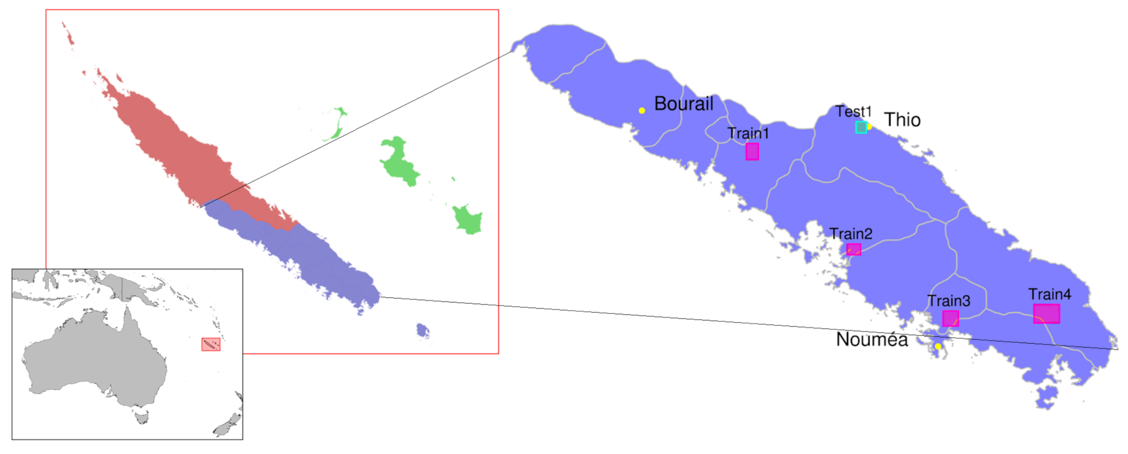
In the South Province, five areas of interest were selected (Figure 1). They are distributed throughout the region and contain a variety of environments, including mining areas, urban areas and tropical forests. They were chosen to, as much as possible, reflect the diversity of the territory. From these zones, data sets were constructed for training, validation, and testing. The description, extent and surface of the five areas are described in the Table 1. The data were projected according to the reference coordinate system RGCN91-93/Lambert New Caledonia (EPSG:3163). In addition to the areas shown in Figure 1, the top left (,) and bottom right (,) coordinates are described in Table 1. These training and testing areas (see Figures S1–S3) can be downloaded and used as benchmarks to compare the LULC classification techniques at [26].
2.2. Data Collection
The SPOT6 data, recorded in the course of 2013–2014, were radiometrically corrected and assembled into a mosaic covering the total area of 18,575 km of New Caledonia. The Red, Green, Blue and Near Infra-Red (RGB and NIR) channels were available at 1.5 m resolution. The data were provided as ortho-rectified tiles based on the local authorities’ 10-meter DTM, for a total of 12 images, which are detailed in Table 2.
A few images were available, explaining the remaining cloud cover (≈10%) despite the mosaic. In addition, the images were acquired early in the morning and, as the Southern Province is a high relief area, the south-southwest oriented hillsides show significant shadows and prevent observation on some mountain sides. As a high tropical island, New Caledonia experiences very little seasonal variation. However, there are periods of drought that can last from 3 to 6 months, so remote sensing images may have large radiometric differences between them despite showing the same LULC. This variation was considered negligible for this study, as Deep Learning normally copes well with multimodal data distributions [27]. It is on the basis of these satellite images that LU and LC labelling was carried out over the five study areas.
2.3. Classification System
There are two main, complementary ways to classify objects on the Earth’s surface: LC, which amounts to the type of physical material visible at a given location, and LU, which categorizes the location according to its function (natural or for human use).
In this study, different classes were delimited by vectors and then labelled according to the two nomenclatures. The classes chosen for the different nomenclatures were directly inspired by the previous work regarding LU accomplished by the New Caledonia Environmental Observatory [11]. This nomenclature is itself based on the CORINE land cover inventory [28].
For LC, a first classification was carried out taking into account only the surface cover, for a total of five classes shown in the Table 3, numbered from 1 to 5 in column L.
For LU, two levels of hierarchy were established. The first level (column L1 of Table 4) separated three classes: the urban or built-up areas, the undeveloped areas, and the wetlands. The second level (column L2 of the Table 4) subdivided each of these classes into several subclasses as presented in the Table 4. These classes were identified in particular for their significance for land management and conservation in New Caledonia and were derived from thematic research conducted by the OEIL which, as previously mentioned, compiled a similar LU nomenclature. For example, mines are common in New Caledonia and need to be closely monitored because of their high potential environmental impact. Identifying them is important for tasks such as monitoring forest fragmentation or preventing soil erosion. Compared to the original nomenclature proposed by OEIL, agricultural land was removed because it was mainly pasture areas, indistinguishable in this form from an area of low-density vegetation by photo-interpretation.
Clouds and shadows were masked in the satellite images and did not appear in the nomenclatures. The cloud mask is a remote sensing product provided with SPOT6 data and shadows can be detected with a simple heuristic approach that searches (almost) black bodies [29]. Subsequently, for Deep Learning architectures, the different classes were renamed from 0 to 12 (column C of the Table 4), where class 0 contained clouds and shadows and was ignored during the learning process.
The LU and LC labelling were carried out jointly through photo interpretation by a unique human operator. This ensured consistent results and also consolidated work, since the two nomenclatures overlapped in a large portion of the territory (in particular, the natural, uncultivated land). The pixel-accurate labelling of the test area is shown in Figure 2.
3. Methods
3.1. Use of Neo-Channels
The four raw channels of SPOT 6 used in this study were recorded in the R, G, B and NIR wavelengths, respectively. On the basis of the characteristics of the raw channels, neo-channels were calculated to highlight the particularity of certain land types in remote sensing [30,31] or complex objects such as urban infrastructures [32]. For example, NDVI [33] was used to highlight vegetation cover. Neo-channels are potentially important for XGBoost because the technique does not have the feature learning capabilities like Deep Learning. The neo-channels used in this study were as follows:
3.2. XGBoost
To serve as baseline, we used a standard machine learning method called XGboost (“Extreme Gradient Boosting”, [39]). It is a boosting scheme with decision trees as base (weak) learners that are combined into a strong learner. XGBoost iteratively builds an ensemble of trees on subsets of the data; weighting their individual predictions according to their performance. An ensemble prediction is then computed by taking the weighted sum of all base learners. The library is designed to be highly efficient and provides parallel algorithms for tree boosting (also known as GBDT, GBM) that are very well suited for the big data of remote sensing. XGboost is a state-of-the-art technique in supervised classification that showed very strong performance on a wide variety of benchmark tasks [39].
To run an XGBoost model, neo-channels and multiple texture filters were used. The filters were: dissimilarity, entropy, homogeneity and mean. Input of windows were used for labeling the central pixel. The training data were the same as for the Deep Learning architectures.
3.3. Deep Learning Architectures
The internal parameters of the employed Convolutional Neural Network (CNN) architectures were not changed with regards to the originally proposed ones. A CNN [40] is a machine learning technique based on sequences of layers of three different types: convolutional, pooling or fully connected layers. Convolution and fully connected layers are usually followed by an element-wise, non-linear activation function.
In the frame of classification of visible satellite data into l classes, the first layer of a Deep Learning architecture receives an input, generally an image of k channels of pixels. The convolutional layers act as filters that extract relevant features from the image. Pooling layers then allow sub-sampling the filter responses to a lower resolution to extract higher-level features with larger spatial context. The last layers map the resulting feature maps to class scores. There are two possible strategies: “central-pixel labeling”, where a fully connected layer maps the features computed over an entire image patch to a vector of (pseudo-)probabilities for only the central pixel of the patch; or “semantic segmentation”, where the high-level features are interpreted as a latent encoding and decoded back to a map of per-pixel probabilities for the entire patch, where the decoder is a further sequence of (up-)sampling and convolution layers. The objective of this coding-decoding sequence is to extract informative data from the inputs, remove the noise signal and combine the information for classification purposes.
All architectures were trained with stochastic gradient descent using a similar protocol, with a momentum of 0.9 and starting from an initial learning rate of . Every 20 epochs, the learning rate is divided by 10 until reaching .
Neural networks do not perform well when trained with unbalanced data sets [41]. In the case of “central-pixel labeling” architectures it is possible to make balanced data sets with the initial pixels selection used for the learning. In the case of “semantic labeling” the composition of the images makes it more difficult to precisely control the number of pixels per class. We tried several methods, but found negligible differences in performance. All reported experiments use the median frequency balancing method.
3.3.1. Central-Pixel Labeling
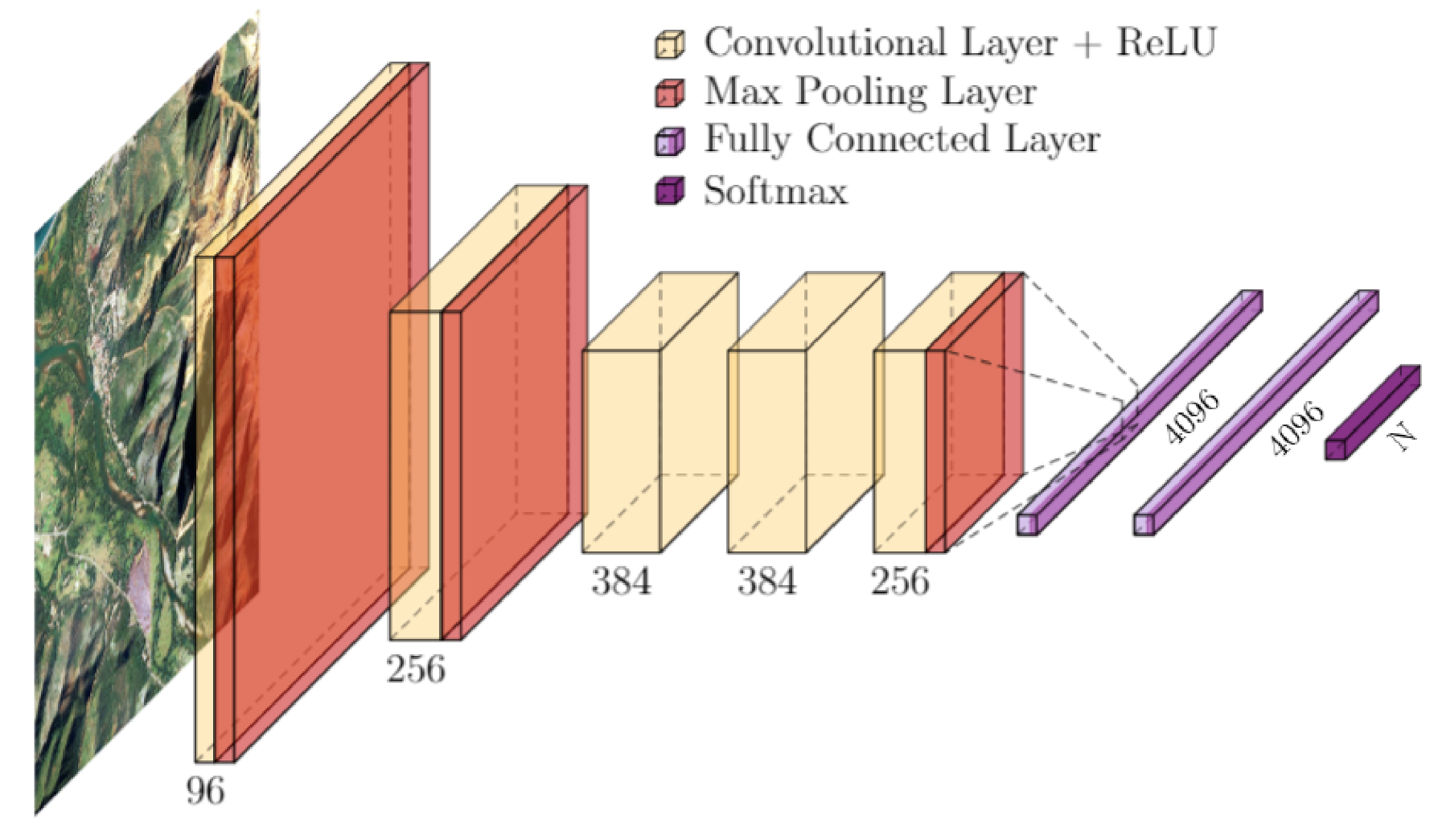
AlexNet, an architecture introduced by Alex Krizhevsky [42], is one of the first Deep Learning architectures to appear on the scene. Inspired by the LeNet architecture introduced by Yann LeCun [40], AlexNet is deeper with eight layers, the first five being convolutional layers whose parameters are shown in Table 5, interleaved with max-pooling layers (Figure 3). The sequence finishes with two fully connected layers before the final classification with a softmax. A ReLu type activation function is used for each layer. Data augmentation and drop-out are used to limit overfitting.
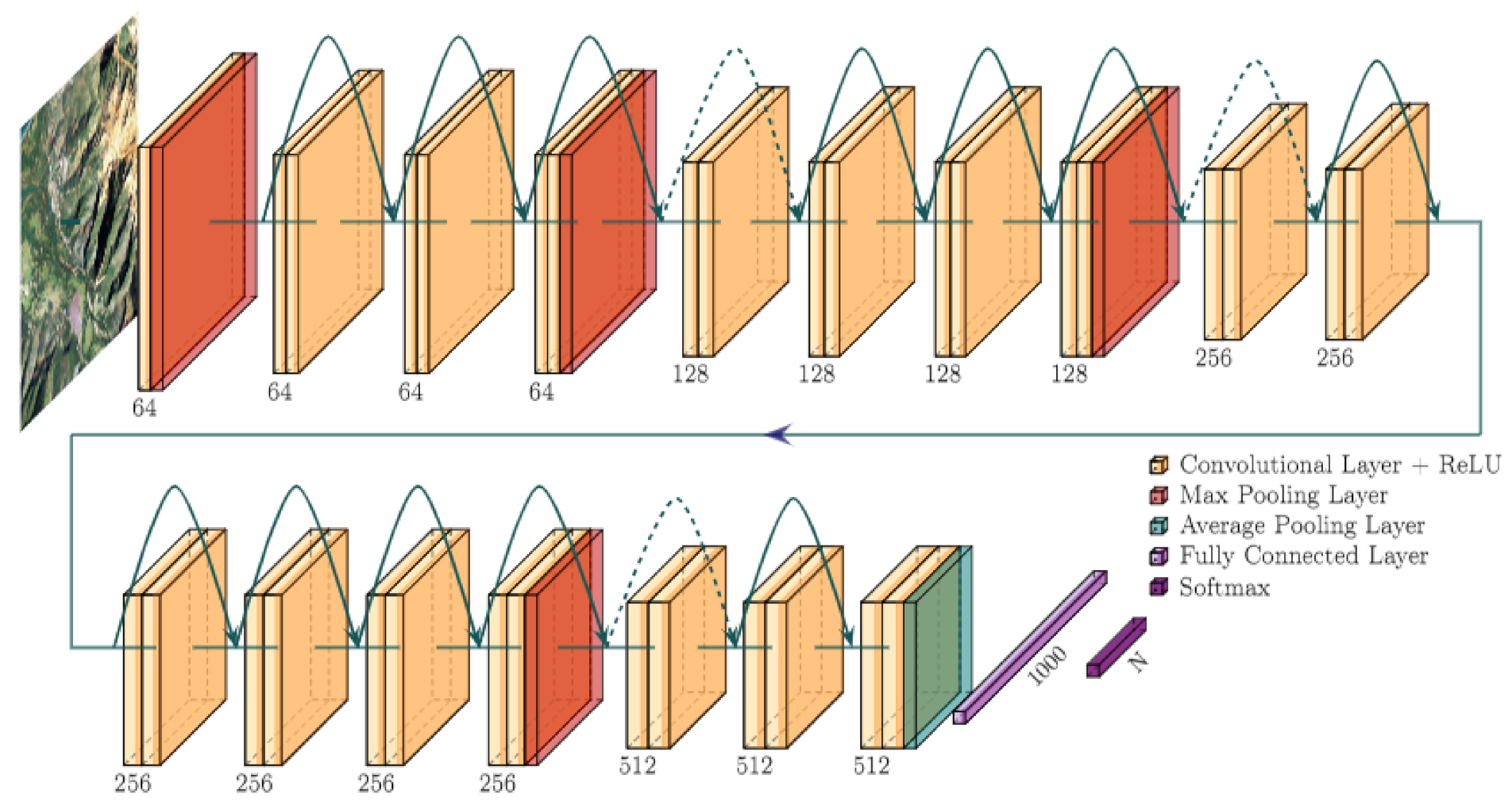
ResNet (Deep Residual Network, [43]) is a Deep Learning architecture with many layers that use skip connections, as illustrated in Figure 4. These skip connections allow the bypassing of layers and add their activations to those of the skipped layers further down the sequence. The dotted arrows in Figure 4 denote skip connections through a linear projection to adapt to the channel depth.
By skipping layers and thus shortening the back-propagation path, the problem of the “vanishing gradient” can be mitigated. Figure 4 represents a 34-layer ResNet architecture. The first layer uses convolutions, the remaining ones .
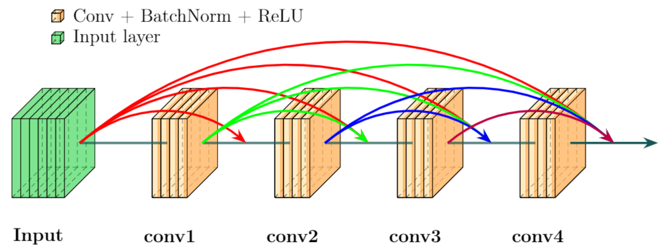
The DenseNet architecture [44] extends the principle of ResNet, with skip connections to all following layers in a module called a “dense block”, as shown in Figure 5. The activation maps of the skipped layers are concatenated as additional channels. The architecture then consists of a succession of convolution layers, dense blocks and average pooling.
3.3.2. Semantic Labelling
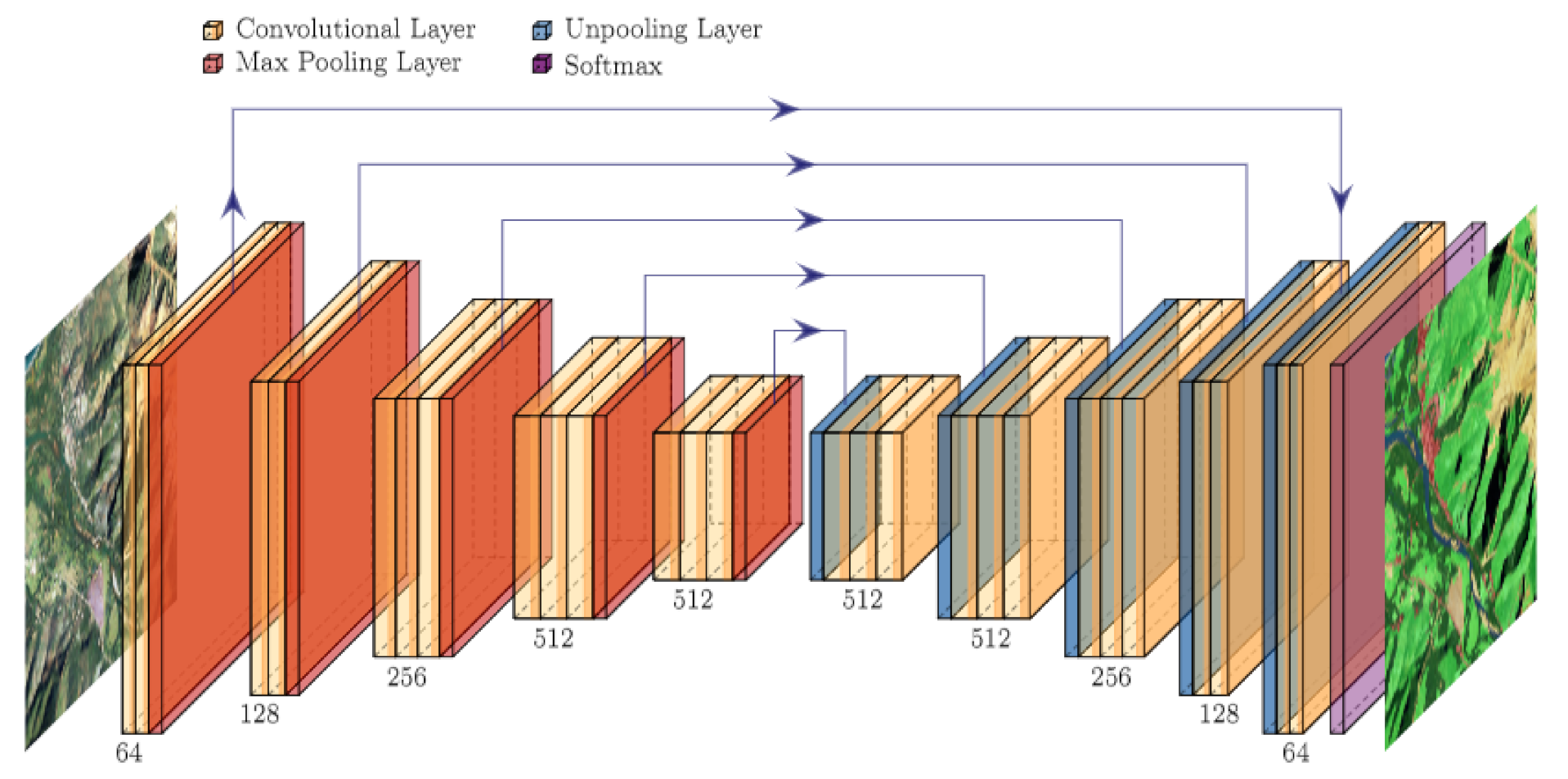
Unlike “pixel labelling”, the “Semantic Labelling” approach classifies all pixels of an image patch to obtain a corresponding label map. For this purpose, the architectures SegNet, DeepLabV3+, and FCN are used. SegNet [45] is a neural network of encoder-decoder types like DeconvNet [46] or U-Net [47]. The encoder in the Deep Learning architecture is a series of convolutional and max pooling layers that encode the image into a latent “feature representation”. Before each pooling step, the activations are also passed to the corresponding up-convolution layer in the decoder, to preserve high-frequency detail (see Figure 6).
The Fully Convolutional Networks (FCNs) [48] have convolution layers instead of fully connected ones, preserving some degree of locality throughout. These layers include two parts: the first part consisting of convolutional and max pooling to fulfil the function of the encoder, and the second part comprises an up-convolution to recover the initial dimensions of the image and a softmax to classify all pixels. In order to maximize recovery of all the information during the encoding, skip connections are included similar to [43] architecture.
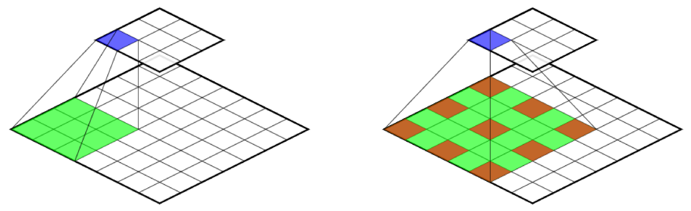
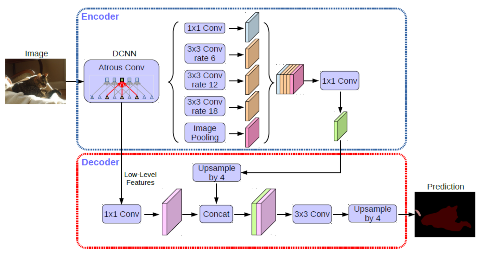
The DeepLab V3+ architecture [49] uses so-called “Atrous Convolution” in the encoder. This makes it possible to apply a convolution filter with “holes”, as shown in Figure 7, covering a larger field of view without smoothing.
Atrous convolution is embedded in a ResNet-101 [50] or Xception [51] architecture, delivering a pyramid of activations with different atrous rates (see Figure 8). This pyramid accounts for objects of different scales and thus increases the expressive power of the model. After appropriate resampling in the decoder, a semantic segmentation is obtained.
3.4. Sampling Method
The SPOT6 satellite data for our five study areas were preprocessed to be fed into the different Deep Learning architectures and the XGBoost model. First, the data were split into three mutually exclusive parts: a learning set, a validation set and a test set totally independent of the two previous ones.
Four of the five areas were used for learning and validation. The last, isolated scene was then used as the test set. It contained all the classes for the two nomenclatures, the five LC classes, and the 12 LU classes. In addition, this image contained all the environments representing the New Caledonian landscape: urban, mining, mountainous and forest environment with variations from the coastline to the inland mountain areas. It is on this entire scene that the final confusion matrix and quality metrics were computed.
Several possible input channel combinations were tested for both XGBoost and Deep Learning. For both LU and LC classification, a set of data consisting only of the four SPOT6 channels (Red, Green, Blue and Near Infra-Red), was used as a basis. The other data sets were composed of these raw channels with six additional neo-channels: NDVI, MSAVI, MNDWI, L, , and ExG.
In addition to these inputs, LC information can also be used to assess whether additional LC information can improve LU classification. To that end we first performed LC mapping, then added the max-likelihood LC label as an input channel for the LU mapping. The different variants are summarized in Table 6.
3.5. Mapping and Confusion Matrix
After fitting the parameters of the different Deep Learning architectures as well as XGBoost on the training set, they were run on the test set to obtain a complete mapping of LC and LU as described above. Confusion matrices were extracted from these results. Four quality metrics are used: Overall Accuracy (OA), Producer Accuracy (PA), User Accuracy (UA) and the F1-score. The OA takes the sum of the diagonal of the confusion matrix. The PA takes the number of well-ranked individuals divided by the sum of the column in the confusion matrix. The UA takes the number of well-ranked individuals divided by the sum of the line. Finally, the F1-score is calculated as the harmonic mean of precision and recall. This last metric allows calculating the accuracy of a model by giving an equal importance between the PA and the UA. Note that the shadow and cloud areas were not taken into account in the confusion matrix.
For architectures using a “central-pixel labeling” method, the mapping was done pixel by pixel using a sliding window with step size 1. In each window only the central pixel (i.e., row 33, column 33 of the window) was classified. To sidestep boundary effects, a buffer of 32 pixels at the boundary of the scene was not classified.
For “semantic labeling” architectures, we empirically used a sliding window with step size 16. With bigger steps the results deteriorated, and smaller ones did not bring further improvements. Every pixel was thus classified multiple times, and we averaged the resulting per-class probabilities. Finally, the class with the highest score was retained as a pixel label.
4. Results
4.1. Evaluation of Land Cover Classification
The nomenclature used for the LC detection is described in Table 3. The comparison of the classification performances of different models (XGBoost, several Deep Learning architectures) is shown in Table 7 with the RGBNIR dataset. The best results for the “central-pixel labeling” and “semantic labeling” methods for each metrics of accuracy are presented in bold. The results on the four training areas for the LC classification are presented in Table A1, Appendix A.
For the LC detection task all tested methods reached overall accuracies between 73% (AlexNet/“central-pixel labeling”) and 81% (Deeplab/“semantic labeling”). The XGboost baseline performed on par with the best Deep Learning methods, except for lightly lower overall accuracy. Excluding the basic AlexNet architecture, most Deep Learning architectures obtained similar performances. Most models showed UA higher than PA, i.e., recall (percentage of total relevant results correctly classified) was higher than precision (percentage of relevant results).
4.2. Evaluation of Land Use Classification
Using the same input channels as in the previous section, the same models were trained for the more complex LU classification task. Here the algorithms had to differentiate between 12 land type classes for the classification, as described in the nomenclature in Table 4. Table 8 presents the results of the LU classification on the test area and Table A2, in the Appendix, presents the results of the LU classification on the four training areas.
For the LU detection task, all deep learning techniques except AlexNet outperformed XGBoost. Differences were significant, with up to 15 percent points in OA. As in the previous section, the best performing “single-pixel” architecture is DenseNet and the best “semantic labeling” network is DeepLab. Interestingly, DenseNet reached the best PA, although DeepLab dominated the remaining metrics.
For the remainder of this study, the best performing “single-pixel” and “semantic labeling” were selected. There was little difference between the architectures, so the architectures with the best F1-score for the LU classification were chosen arbitrarily.
4.3. Influence of Neo-Channels and Land Cover as Input on the Learning
The first part of Table 9 presents the results of the two strongest architectures, DenseNet and DeepLab, when neo-channels were used as input. In most cases, adding neo-channels made little difference. Still, although feature learning should theoretically be able to approximate them, some channel combinations did lead to noticeable improvements, typically involving the channel. Very few datasets managed to outperforme the initial RGBNIR dataset by more than on the different accuracy metrics (bold figures in Table 9). Similar results were observed for the LC task.
The best performing architectures were selected and used for an LU detection task with the LC as input on top of the raw channels. We ran two variants, an LCM (Land Cover Model) which used the LC predictions of the deep learning model; and an LCE (Land Cover Expert), which used the ground truth values, i.e., this version served as an upper bound of what LU performance could be if a perfect predictor for LC was available (see Table 9).
Due to the closeness between certain LC and LU classes (e.g., forest), LCE achieved results closer to 75% of OA for both architectures. Note that this is an upper bound of how much LU information can be extracted from known LC, hinting at the complexity of the problem and the limits of deriving LU only from image data.
More interestingly, we also observed improved LU classification when adding LC labels as additional input to the architecture. The two-step approach appeared to simplify the task. At this stage it is not completely clear why that was the case, as the LC labels are obviously information that the respective architecture could find on its own, and the high performance of XGBoost makes it unlikely that extracting the LC labels exhausted the capacity of the chosen architectures. A gain was also observed for the OA and the UA when the LCM was added as input to the model, with similar results for the PA.
4.4. Confusion Matrix of the Best Deep Learning Model for LULC Classification
The results of the best performing architecture for the LULC classification task, DeepLab, is detailed with two confusion matrices. Table 10 shows The LC classification task with the raw channels as input, and the LU classification task with the LCE in addition to the raw channels, is in Table 11. The resulting maps of the LU labelling task are shown in Figure 9.
5. Discussion
In New Caledonia, for both LC detection and LU detection, the best Deep Learning techniques show good performance in overall detection accuracy on the test set relative to a human operator (respectively 81.41% and 63.61%). The two baseline techniques: XGBoost and AlexNet, are easy to implement and require low CPU time consumption. They achieved satisfactory performance on the LC classification (respectively 77.55% and 73.29%) task in New Caledonia but, as expected, showed their limitations for the challenging LU classification task (respectively 51.56% and 45.79%), with XGBoost performing slightly better on both tasks. In this particular case, standard remote sensing classification techniques using neo-channels and textures were slightly more effective than a basic deep learning architecture (AlexNet) using raw channels as input.
When using more advanced Deep Learning architectures, a clear improvement appeared. While the differences were rather small for LC classification, quite important gains could be obtained for LU by selecting the right architecture. In this study, two types of architectures were tested: “semantic labelling” architecture and “pixel labelling” architecture. Among them, DeepLab (“semantic labelling”) and DenseNet (“pixel labelling”) stood out and showed similar results. The “pixel labeling” architectures outperform the “semantic labeling” ones on the training set presented in the appendix. However, these architectures have equal performances on the test set. The “pixel labeling” architectures seem to be more sensitive to overfitting, especially the ResNet architecture.
Nevertheless, due to lower CPU time consumption, it could be interesting to use a “semantic labeling” approach when dealing with very high resolution remote sensing images. Furthermore, the resulting LULC maps from the “pixel labelling” architectures are usually noisy with many isolated pixels surrounded by pixels from a different class. The resulting frontiers between classes can look fuzzy. On the contrary, the maps generated by the “semantic labelling” are much more homogeneous, though the surfaces of the predicted classes depend on the size of the chosen sliding window for subsampling the area and do not respect the observed frontiers between classes.
In this study, even if we used a balanced data set for training, none of the four training areas contained all classes of the LULC nomenclature; only the area Test1 (Table 1) included all possible labels. Indeed, there are great inequalities in the distribution of classes, with the vegetation class covering more than 90% of the New Caledonian territory. The test set was used as is, without any class balancing, so as to correspond to a realistic, complete mapping task.
The accuracy of LC classification was globally high with a global accuracy of 81.41% on the test set for the best model. Table 10 showed that the building class detection was the most difficult task in this study. The model tended to overestimate the extent of this class, creating many false positives on other classes, especially on bare soil. This could be explained by the proximity of these classes around buildings (Figure 9).
A slight confusion between forest and low density vegetation, as well as between bare soil and low density vegetation was also noted. However, distinguishing these classes is a difficult task even for a human operator. It should be noted that at this scale it was not possible to provide accurate field data. Most of the boundaries between classes were established by photo-interpretation. Unlike other learning tasks that are rely on perfectly controlled data, the train and test data sets for LULC classification are never error-free. It is therefore difficult to know whether classification errors are due to a lack of model performance or to mislabeling.
The LU and LC were fairly similar because of the many areas not subject to direct human use. The main differences occurred in the division of the urban fabric. It is far more complex to qualify this type of area, and human expertise is often necessary but subjective. For example, the difference in urban fabric between residential and industrial areas is open to misinterpretation. One might think that buildings with very large roofs, such as warehouses, belong to the industrial class, but this classification quickly becomes subjective, as schools, sports complexes, etc. also correspond to this criterion but, belong to the residential area. Only on-the-ground knowledge would remove these ambiguities.
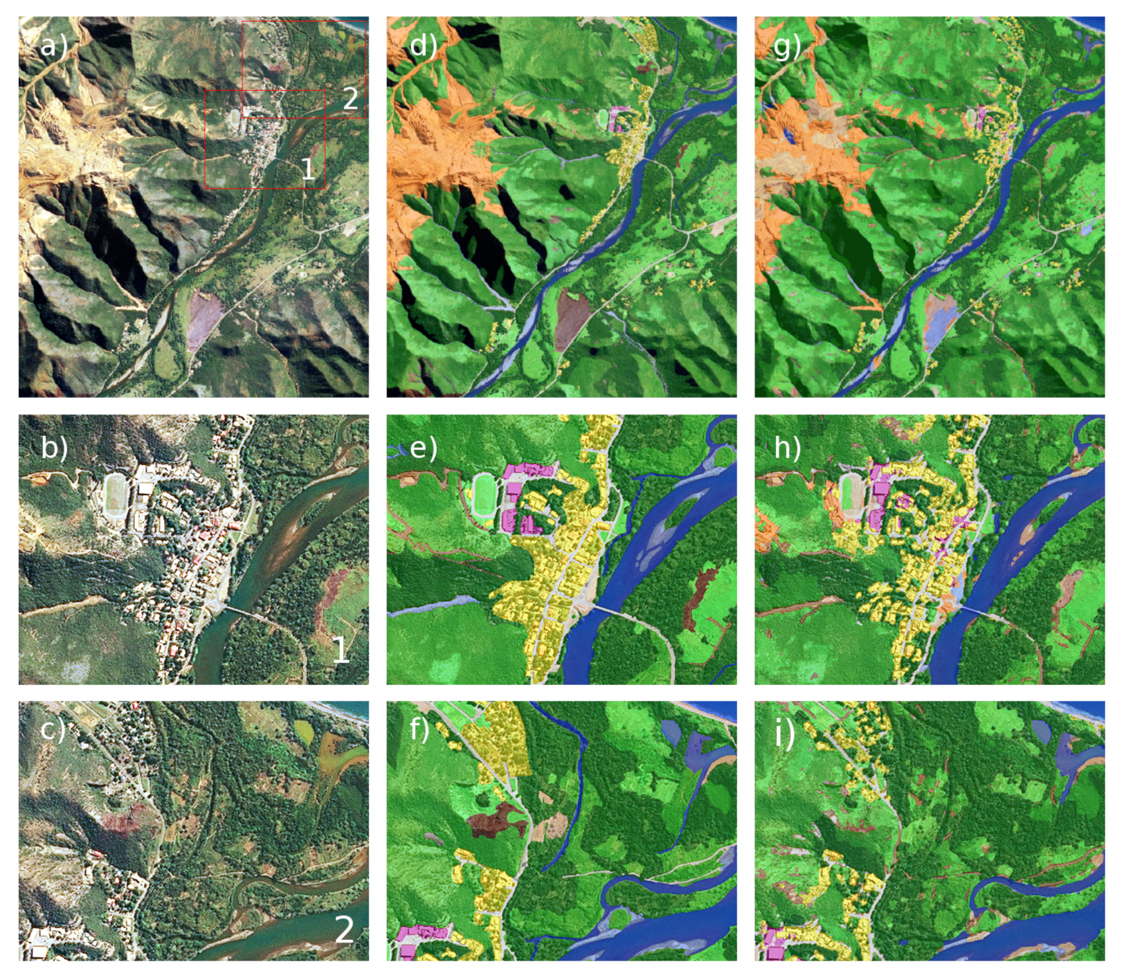
The LU classification remained a very challenging task with the score of 63.61% on the test set for the best deep learning architecture with a clear improvement compared to XGBoost (51.56%). The water surfaces and worksites were well detected by the model, but the other classes such as trails, bare rocks, and bare soil had very low recognition rates (see Table 11). Indeed, from a radiometric point of view, it is difficult to distinguish a trail from bare ground. Distinguishing between these classes requires a broad knowledge of the ground and a high level of cognitive reasoning (a trail is a bare ground 3 to 5 m wide with a particular wire form). We hoped that Deep Learning models would be able to distinguish this type of class, but it seems that there was not enough extra information in our data set to handle this task accurately (such as exogenous information or large-scale vision). The same difficulty then stood for engravement and bare soil classes. Moreover, the Deep Learning techniques barely distinguished mines and bare soil classes, but this task is very difficult to perform, even for a human operator, without contextual information and based only on a small picture ( pixels).
As stated in the introduction, a major challenge is to monitor the forest area, as a spatial understanding of biomass and carbon stock in tropical forests. It is crucial for assessing the global carbon budget. Similarly, detecting the bare soil area changes is an important task in order to limit the erosion. The accuracy of detection for the Forest class reached 0.78 as detailed in Table 10. This class can be confused with the Low-density vegetation class (19% of mislabeling between those two classes) and the Bare Soil class was similarly confused with the Low-density vegetation class (14% of mislabeling). For those specific classes, these results are significantly better than those obtained with the machine learning techniques (gain around 10% of accuracy) and the monitoring of forest and bare soil areas would be significantly improved using deep learning techniques.
Even with all these imperfections on the train and test set, the results showed there is a real added value in using Deep Learning techniques in the frame of LULC detection in a complex environment such as a tropical island. The Deep Learning architectures were applied to a completely different geographic region in the Southern Province and with a different climate (area located east of the mountain range and exposed to rain and wind), they overcame these challenges with up to 80% accuracy for the LC classification task. Other Deep Learning applications on LC manage to achieve similar results [52,53].
Unlike the “Corine Land Cover” classification, the agriculture areas class do not appear in the Level 1 (L1) and Level 2 (L2) nomenclature since this class could not be distinguished using standard deep learning approaches from low-density vegetation class. Likely, this is due to the size of the sliding window, not large enough to catch the features that can be computed to distinguish the two classes. Further work based on a multiscale approach could be useful to overcome this issue.
Our findings also showed that adding the LC output as input for the LU classification can improve the accuracy, suggesting that it could be interesting to perform a hierarchical approach for the LULC task. This hierarchy of concept could also be used to improve the interpretability and explicability of results. Indeed, understanding how Deep Learning combines information to effectively classify land use classes remains a challenging task, but recent research using ontologies could be useful to achieve this goal [54]. This idea could also highlight missing exogenous information (elevation, cadastre, etc.) in addition to remote sensing data to improve LULC detection. Unifying the most difficult classes to detect could improve the performance of the LU classification results. The difficult classes would then be moved to a different, more accurate level of the classification, for example, an L3 level in Table 4. Another path for improvement consists in including cloud and shadow detection in the classifier and using post-processing filters [55] and heuristics (object-oriented rules…).
These results presented here seem robust since, at a resolution of 1.5 meters and for an image of pixels, the receptive field equals approximately 0.01 km. At this resolution and area, it is possible for a human operator to identify the type of land and its use. We investigated alternative sizes of pixels or pixels, with step size 8, and dimilar results were obtained. Due to hardware limitations of the graphic card, implying a drastic reduction of the batch size, we did not further pursue the pixel configuration. The larger number of individual samples at size did not seem to make much difference. Hence, we settled for pixels, striking a compromise between image size and number of samples.
6. Conclusions
In this study, machine learning techniques such as Deep Learning and XGBoost were compared for LULC classification in a tropical island environment. For this purpose, a specific data set based on SPOT6 satellite data was created and made available for the scientific community, comprised of five representative areas of New Caledonia labelled by a human operator: four used as training set, and the fifth one as test set [26]. The performance of XGBoost managed to stand up to Deep Learning for LC classifications but, as for many applications in image processing, the best deep learning architectures provided the best performances. The standard machine learning approach is clearly behind on the more complex LU domains which require a higher level of conceptualization of the surroundings to obtain good results. Though the framework can be complex to handle, the Deep Learning approach for LULC detection was easy to implement since there is no significant gain to pre-process the data by computing neo-channel or texture-based input in contrast to conventional remote sensing techniques.
Specific to the deep learning approach, the two methods: “semantic” labeling and “pixel labeling” provided equivalent performances for the most efficient architectures: DeepNet and DeepLab, whose internal structure was not modified.
Our findings also showed that adding the LC output as input for the LU classification improved the accuracy, suggesting that a hierarchical approach could be interesting to perform the LULC task. Further work on this classification is necessary to obtain better results, but it is a step forward towards the development of an automatic system allowing the monitoring of the impact of human activities on the environment by the detection of the forest surface change and bare soil areas.
In future work, we aim to apply the classifier to the rest of New Caledonia, including the Northern Province and the Islands Province. Additional information will be necessary to cover the specific conditions in those new regions. In terms of mapping area, it may be interesting to also include the maritime environment, in particular the many islets and reefs of the New Caledonian lagoon. We also plan to adapt the classification to use Sentinel-2 instead of SPOT6 as input for LULC classification. While the Sentinel-2 sensor has lower spatial resolution, its spectral resolution is better and it offers a revisit times of only 5 days.
Supplementary Materials
The following are available online at https://www.mdpi.com/article/10.3390/rs13122257/s1, Figure S1: SPOT 6 remote sensing images of the five areas of interest, Figure S2: LC labelling of the five areas of interest, Figure S3: LU labelling of the five areas of interest.
Author Contributions
Conceptualization, G.R., M.M., K.S., M.D.; data curation, G.R., M.D.; methodology, G.R., M.M., K.S.; software, G.R., M.M.; validation, G.R., M.M.; writing—original draft, G.R., M.M.; writing—review and editing, M.D., K.S. All authors have read and agreed to the submitted version of the manuscript.
Funding
This research received no external funding.
Data Availability Statement
The data presented in this study are openly available in SPOT6 satellite imagery, land cover and land use classification of 5 areas in the South Province of New Caledonia at https://doi.org/10.23708/PHVOJD.
Conflicts of Interest
The authors declare no conflict of interest.
Appendix A

Table A1.
Results of Deep Learning architecture and XGBoost for the LC detection task with RGBNIR as input on the training set.
Table A1.
Results of Deep Learning architecture and XGBoost for the LC detection task with RGBNIR as input on the training set.
| Architectures | OA | PA | UA | F1-Score |
|---|---|---|---|---|
| XGboost | 80.26% | 81.91% | 82.73% | 82.23% |
| AlexNet | 93.00% | 92.78% | 93.96% | 93.37% |
| ResNet | 99.00% | 99.33% | 99.31% | 99.32% |
| DenseNet | 99.00% | 99.35% | 99.09% | 99.22% |
| SegNet | 94.57% | 96.08% | 91.33% | 93.64% |
| DeepLab | 94.64% | 96.03% | 93.91% | 94.96% |
| FCN | 95.84% | 96.90% | 94.54% | 95.71% |
Table A2.
Results of Deep Learning architecture and XGBoost for the LU detection task with RGBNIR as input on the training set.
Table A2.
Results of Deep Learning architecture and XGBoost for the LU detection task with RGBNIR as input on the training set.
| Architectures | OA | PA | UA | F1-Score |
|---|---|---|---|---|
| XGboost | 59.29% | 59.13% | 54.26% | 56.59% |
| AlexNet | 82.00% | 84.08% | 79.37% | 81.66% |
| ResNet | 95.00% | 96.54% | 95.69% | 96.12% |
| DenseNet | 96.00% | 96.58% | 96.41% | 96.49% |
| SegNet | 78.79% | 66.74% | 70.16% | 68.41% |
| DeepLab | 86.58% | 89.94% | 81.63% | 85.59% |
| FCN | 85.34% | 89.30% | 78.87% | 83.76% |
References
- Veldkamp, A.; Lambin, E. Predicting land-use change. Agric. Ecosyst. Environ. 2001, 85, 1–6. [Google Scholar] [CrossRef]
- Wilson, J.S.; Clay, M.; Martin, E.; Stuckey, D.; Vedder-Risch, K. Evaluating environmental influences of zoning in urban ecosystems with remote sensing. Remote Sens. Environ. 2003, 86, 303–321. [Google Scholar] [CrossRef]
- Lary, D.J.; Alavi, A.H.; Gandomi, A.H.; Walker, A.L. Machine learning in geosciences and remote sensing. Geosci. Front. 2015, 7, 3–10. [Google Scholar] [CrossRef] [Green Version]
- Blaschke, T. Object based image analysis for remote sensing. ISPRS J. Photogramm. Remote Sens. 2010, 65, 2–16. [Google Scholar] [CrossRef] [Green Version]
- Chazeau, J. Research on New Caledonian Terrestrial Fauna: Achievements and Prospects. Biodivers. Lett. 1993, 1, 123–129. [Google Scholar] [CrossRef]
- Isnard, S.; L’huillier, L.; Rigault, F.; Jaffré, T. How did the ultramafic soils shape the flora of the New Caledonian hotspot? Plant Soil 2016, 403, 53–76. [Google Scholar] [CrossRef]
- Dumas, P.; Printemps, J.; Mangeas, M.; Luneau, G. Developing erosion models for integrated coastal zone management: A case study of The New Caledonia west coast. Mar. Pollut. Bull. 2010, 61, 519–529. [Google Scholar] [CrossRef]
- Grandcolas, P.; Murienne, J.; Robillard, T.; Desutter-Grandcolas, L.; Jourdan, H.; Guilbert, E.; Deharveng, L. New Caledonia: A very old Darwinian island? Phil. Trans. R. Soc. B 2008, 363, 3309–3317. [Google Scholar] [CrossRef] [Green Version]
- Pelletier, B. Geology of the New Caledonia region and its implications for the study of the New Caledonian biodiversity. In Compendium of Marine Species from New Caledonia, 2nd ed.; Payri, C., Richer de Forges, B., Colin, F., Eds.; Documents Scientifiques et Techniques: II, IRD: Nouméa, France, 2007; pp. 19–32. Available online: https://www.documentation.ird.fr/hor/fdi:010059749 (accessed on 1 June 2021).
- Pellens, R.; Grandcolas, P. Conservation and Management of the Biodiversity in a Hotspot Characterized by Short Range Endemism and Rarity: The Challenge of New Caledonia. In Biodiversity Hotspots; Rescigno, V., Maletta, S., Eds.; Nova Science Publishers: Hauppage, NY, USA, 2010; pp. 139–151. [Google Scholar]
- Rolland, A.K.; Crépin, A.; Kenner, C.; Afro, P. Production de Données D’Occupation du sol 2010–2014 sur la Province Sud. 2017. Available online: http://oeil.nc/cdrn/index.php/resource/bibliographie/view/27689 (accessed on 2 February 2020).
- Deng, L.; Yu, D. Deep Learning: Methods and Applications. Found. Trends Signal Process. 2014, 7, 197–387. [Google Scholar] [CrossRef] [Green Version]
- Cohen, N.; Sharir, O.; Shashua, A. On the Expressive Power of Deep Learning: A Tensor Analysis. In 29th Annual Conference on Learning Theory; Feldman, V., Rakhlin, A., Shamir, O., Eds.; PMLR: Columbia University: New York, NY, USA, 2016; Volume 49, pp. 698–728. [Google Scholar]
- Zhao, Z.; Zheng, P.; Xu, S.; Wu, X. Object Detection With Deep Learning: A Review. IEEE Trans. Neural Netw. Learn. Syst. 2019, 30, 3212–3232. [Google Scholar] [CrossRef] [Green Version]
- Schmidhuber, J. Deep Learning in Neural Networks: An Overview. Neural Netw. 2015, 61, 85–117. [Google Scholar] [CrossRef] [Green Version]
- Hadjimitsis, D.G.; Clayton, C.R.I.; Hope, V.S. An assessment of the effectiveness of atmospheric correction algorithms through the remote sensing of some reservoirs. Int. J. Remote Sens. 2004, 25, 3651–3674. [Google Scholar] [CrossRef]
- Teillet, P.M. Image correction for radiometric effects in remote sensing. Int. J. Remote Sens. 1986, 7, 1637–1651. [Google Scholar] [CrossRef]
- Vicente-Serrano, S.M.; Pérez-Cabello, F.; Lasanta, T. Assessment of radiometric correction techniques in analyzing vegetation variability and change using time series of Landsat images. Remote Sens. Environ. 2008, 112, 3916–3934. [Google Scholar] [CrossRef]
- Zhang, L.; Zhang, L.; Kumar, V. Deep learning for Remote Sensing Data. IEEE Geosci. Remote Sens. Mag. 2016, 4, 22–40. [Google Scholar] [CrossRef]
- Cheng, G.; Han, J.; Lu, X. Remote Sensing Image Scene Classification: Benchmark and State of the Art. Proc. IEEE 2017, 105, 1865–1883. [Google Scholar] [CrossRef] [Green Version]
- Pascal, M.; Richer De Forges, B.; Le Guyader, H.; Simberloff, D. Mining and Other Threats to the New Caledonia Biodiversity Hotspot. Conserv. Biol. 2008, 22, 498–499. [Google Scholar] [CrossRef]
- Mittermeier, R.A.; Werner, T.B.; Lees, A. New Caledonia—A conservation imperative for an ancient land. Oryx 1996, 30, 104–112. [Google Scholar] [CrossRef] [Green Version]
- Georganos, S.; Grippa, T.; Vanhuysse, S.; Lennert, M.; Shimoni, M.; Wolff, E. Very High Resolution Object-Based Land Use–Land Cover Urban Classification Using Extreme Gradient Boosting. IEEE Geosci. Remote Sens. Lett. 2018, 15, 607–611. [Google Scholar] [CrossRef] [Green Version]
- Maillard, P. Comparing texture analysis methods through classification. Photogramm. Eng. Remote Sens. 2003, 69, 357–367. [Google Scholar] [CrossRef] [Green Version]
- GIE OCEANIDE; Jérémy, A.; Antoine, W.; OEIL. L’évolution des Paysages en Province sud. 2012. Available online: https://www.oeil.nc/cdrn/index.php/resource/bibliographie/view/2322 (accessed on 12 March 2020).
- Rousset, G. SPOT6 Satellite Imagery, Land Cover and Land Use Classification of 5 Areas in the South Province of New Caledonia. Version Provisoire. 2021. https://doi.org/10.23708/PHVOJD (accessed on 12 March 2020).
- Gao, J.; Li, P.; Chen, Z.; Zhang, J. A Survey on Deep Learning for Multimodal Data Fusion. Neural Comput. 2020, 32, 829–864. [Google Scholar] [CrossRef]
- Heymann, Y.; Steenmans, C.; Croisille, G.; Bossard, M.; Lenco, M.; Wyatt, B.; Weber, J.L.; O’Brian, C.; Cornaert, M.H.; Sifakis, N. Corine Land Cover Technical Guide; Office for Official Publications of the European Communities: Luxembourg, 1994. [Google Scholar]
- Adeline, K.; Chen, M.; Briottet, X.; Pang, S.; Paparoditis, N. Shadow detection in very high spatial resolution aerial images: A comparative study. ISPRS J. Photogramm. Remote Sens. 2013, 80, 21–38. [Google Scholar] [CrossRef]
- Ngo, T.T.; Collet, C.; Mazet, V. Détection simultanée de l’ombre et la végétation sur des images aériennes couleur en haute résolution. Trait. Signal 2014, 32, 311–333. [Google Scholar] [CrossRef]
- Myneni, R.B.; Hall, F.G.; Sellers, P.J.; Marshak, A.L. The interpretation of spectral vegetation indexes. IEEE Trans. Geosci. Remote Sens. 1995, 33, 481–486. [Google Scholar] [CrossRef]
- Xu, Y.; Wu, L.; Xie, Z.; Chen, Z. Building Extraction in Very High Resolution Remote Sensing Imagery Using Deep Learning and Guided Filters. Remote Sens. 2018, 10, 144. [Google Scholar] [CrossRef] [Green Version]
- Rouse, J.W.; Haas, R.H.; Schell, J.A.; Deering, D. Monitoring the vernal advancement and retrogradation (green wave effect) of natural vegetation. Prog. Rep. RSC 1978-1 1973, 371, 112. [Google Scholar]
- Gevers, T.; Smeulders, A.W.M. Color-based object recognition. Pattern Recognit. 1999, 32, 453–464. [Google Scholar] [CrossRef] [Green Version]
- Qi, J.; Chehbouni, A.; Huete, A.R.; Kerr, Y.H.; Sorooshian, S. A modified soil adjusted vegetation index. Remote Sens. Environ. 1994, 48, 119–126. [Google Scholar] [CrossRef]
- Woebbecke, D.M.; Meyer, G.E.; Von Bargen, K.; Mortensen, D.A. Color indices for weed identification under various soil, residue, and lighting conditions. Trans. ASAE 1994, 38, 259–269. [Google Scholar] [CrossRef]
- Xu, H. Modification of normalised difference water index (NDWI) to enhance open water features in remotely sensed imagery. Int. J. Remote Sens. 2006, 27, 3025–3033. [Google Scholar] [CrossRef]
- Meyer, G.E.; Neto, J.C. Verification of color vegetation indices for automated crop imaging applications. Comput. Electron. Agric. 2008, 63, 282–293. [Google Scholar] [CrossRef]
- Chen, T.; Guestrin, C. XGBoost: A Scalable Tree Boosting System. In Proceedings of the 22nd ACM Sigkdd International Conference on Knowledge Discovery and Data Mining; Association for Computing Machinery: New York, NY, USA, 2016; pp. 785–794. [Google Scholar]
- LeCun, Y.; Bottou, L.; Bengio, Y.; Haffner, P. Gradient-based learning applied to document recognition. Proc. IEEE 1998, 86, 2278–2323. [Google Scholar] [CrossRef] [Green Version]
- Buda, M.; Maki, A.; Mazurowski, M.A. A systematic study of the class imbalance problem in convolutional neural networks. Neural Netw. 2017, 106, 1–23. [Google Scholar] [CrossRef] [Green Version]
- Krizhevsky, A.; Sutskever, I.; Hinton, G. Imagenet classification with deep convolutional neural networks. Adv. Neural Inf. Process. Syst. 2012, 25, 1097–1105. [Google Scholar] [CrossRef]
- He, K.; Zhang, X.; Ren, S.; Sun, J. Deep Residual Learning for Image Recognition. In 2016 IEEE Conference on Computer Vision and Pattern Recognition (CVPR); IEEE Computer Society: Los Alamitos, CA, USA, 2016; pp. 770–778. [Google Scholar]
- Huang, G.; Liu, Z.; Weinberger, K.Q. Densely Connected Convolutional Networks. In 2017 IEEE Conference on Computer Vision and Pattern Recognition (CVPR); IEEE Computer Society: Los Alamitos, CA, USA, 2016; pp. 2261–2269. [Google Scholar]
- Badrinarayanan, V.; Kendall, A.; Cipolla, R. SegNet: A Deep Convolutional Encoder-Decoder Architecture for Image Segmentation. IEEE Trans. Pattern Anal. Mach. Intell. 2017, 39, 2481–2495. [Google Scholar] [CrossRef]
- Noh, H.; Hong, S.; Han, B. Learning deconvolution network for semantic segmentation. In Proceedings of the IEEE International Conference on Computer Vision; IEEE Computer Society: Los Alamitos, CA, USA, 2015; pp. 1520–1528. [Google Scholar]
- Ronneberger, O.; Fischer, P.; Brox, T. U-net: Convolutional networks for biomedical image segmentation. In Medical Image Computing and Computer-Assisted Intervention—MICCAI 2015; Navab, N., Hornegger, J., Wells, W.M., Frangi, A.F., Eds.; Springer International Publishing: Cham, Switzerland, 2015; pp. 234–241. [Google Scholar]
- Long, J.; Shelhamer, E.; Darrell, T. Fully convolutional networks for semantic segmentation. In 2015 IEEE Conference on Computer Vision and Pattern Recognition (CVPR); IEEE Computer Society: Los Alamitos, CA, USA, 2015; pp. 3431–3440. [Google Scholar]
- Chen, L.C.; Papandreou, G.; Kokkinos, I.; Murphy, K.; Yuille, A.L. DeepLab: Semantic Image Segmentation with Deep Convolutional Nets, Atrous Convolution, and Fully Connected CRFs. IEEE Trans. Pattern Anal. Mach. Intell. 2018, 40, 834–848. [Google Scholar] [CrossRef]
- He, K.; Zhang, X.; Ren, S.; Sun, J. Identity mappings in deep residual networks. In Computer Vision—ECCV 2016; Leibe, B., Matas, J., Sebe, N., Welling, M., Eds.; Springer International Publishing: Cham, Switzerland, 2016; pp. 630–645. [Google Scholar]
- Chollet, F. Xception: Deep learning with depthwise separable convolutions. In 2017 IEEE Conference on Computer Vision and Pattern Recognition (CVPR); IEEE Computer Society: Los Alamitos, CA, USA, 2017; pp. 1251–1258. [Google Scholar]
- Feng, J.; Chen, J.; Liu, L.; Cao, X.; Zhang, X.; Jiao, L.; Yu, T. CNN-based multilayer spatial—Spectral feature fusion and sample augmentation with local and nonlocal constraints for hyperspectral image classification. IEEE J. Sel. Top. Appl. Earth Obs. Remote Sens. 2019, 12, 1299–1313. [Google Scholar] [CrossRef]
- Wang, J.; Zheng, Y.; Wang, M.; Shen, Q.; Huang, J. Object-Scale Adaptive Convolutional Neural Networks for High-Spatial Resolution Remote Sensing Image Classification. IEEE J. Sel. Top. Appl. Earth Obs. Remote Sens. 2020, 14, 283–299. [Google Scholar] [CrossRef]
- Confalonieri, R.; Weyde, T.; Besold, T.R.; del Prado Martín, F.M. Using ontologies to enhance human understandability of global post-hoc explanations of black-box models. Artif. Intell. 2021, 296, 103471. [Google Scholar] [CrossRef]
- Su, T.C. A filter-based post-processing technique for improving homogeneity of pixel-wise classification data. Eur. J. Remote Sens. 2016, 49, 531–552. [Google Scholar] [CrossRef] [Green Version]
Figure 1.
Map of New Caledonia and its Provinces (in blue the South Province, in red the North Province and in green the Islands Province). The South Province, zoomed in on the right, shows the four areas selected for the training (in magenta) and the area selected for the test (in cyan).
Figure 1.
Map of New Caledonia and its Provinces (in blue the South Province, in red the North Province and in green the Islands Province). The South Province, zoomed in on the right, shows the four areas selected for the training (in magenta) and the area selected for the test (in cyan).

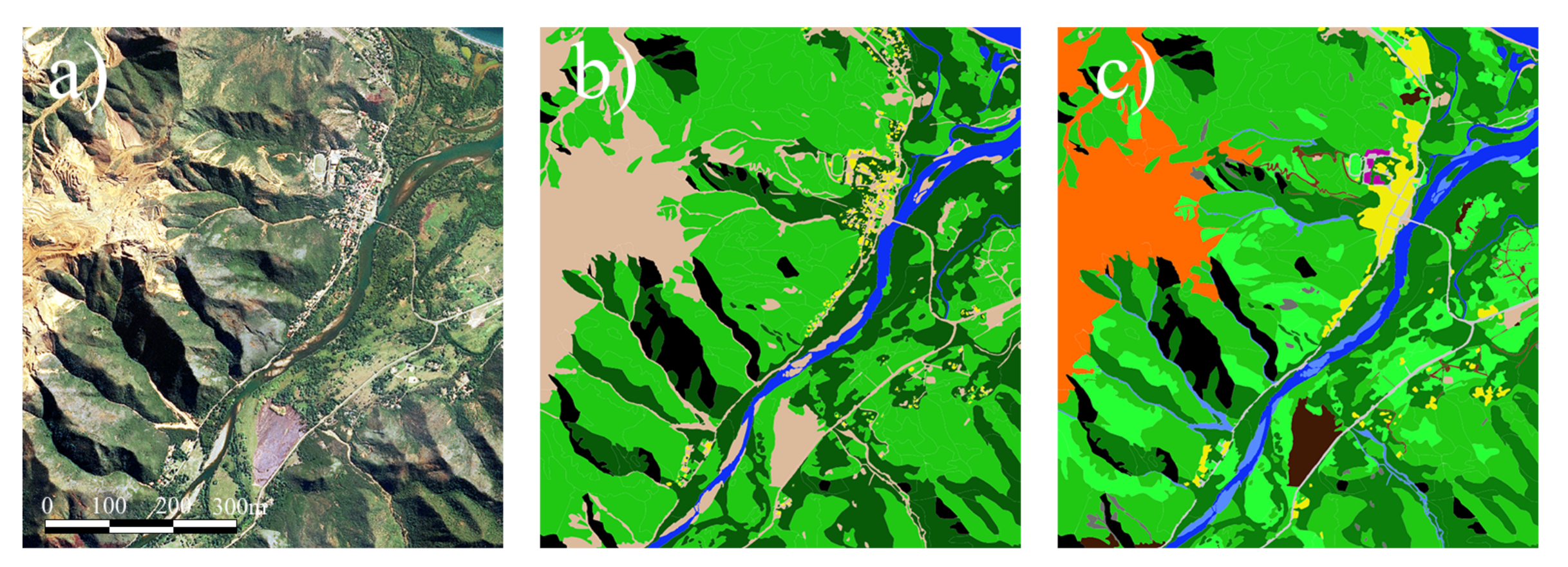
Figure 2.
(a) SPOT6 remote sensing image ( pixels), (b) manually classified according to the LC nomenclature Table 3 and (c) according to the LU nomenclature Table 4. The black pixels represent the mask layer brought by clouds and shadows.

Figure 3.
The AlexNet architecture. The number of kernels is indicated at the bottom of each convolution layer, the rest of the parameters are indicated in Table 5.
Figure 3.
The AlexNet architecture. The number of kernels is indicated at the bottom of each convolution layer, the rest of the parameters are indicated in Table 5.

Figure 4.
Illustration of a ResNet architecture, the arrows above the layers depicting the “skip connections” in the architecture. The number of kernels is indicated at the bottom of each convolution layer.
Figure 4.
Illustration of a ResNet architecture, the arrows above the layers depicting the “skip connections” in the architecture. The number of kernels is indicated at the bottom of each convolution layer.

Figure 5.
Illustration of a dense block. The different colored arrows represent the skip connection made at different levels of the dense block.
Figure 5.
Illustration of a dense block. The different colored arrows represent the skip connection made at different levels of the dense block.

Figure 6.
SegNet architecture. The number of kernels is indicated at the bottom of each convolution layer. The arrows represent the activation layers used as inputs to the corresponding up-convolution layers.
Figure 6.
SegNet architecture. The number of kernels is indicated at the bottom of each convolution layer. The arrows represent the activation layers used as inputs to the corresponding up-convolution layers.

Figure 7.
(left) The normal function of a convolution layer or an Atrous convolution with a separation of 1. (right) An atrous convolution with a separation rate of 6, only the red square will be used to calculate the result (blue square).
Figure 7.
(left) The normal function of a convolution layer or an Atrous convolution with a separation of 1. (right) An atrous convolution with a separation rate of 6, only the red square will be used to calculate the result (blue square).

Figure 8.
DeepLab architecture illustration from the paper [49] showing the internal structure of the architecture, in particular the activation pyramid present in the encoder.
Figure 8.
DeepLab architecture illustration from the paper [49] showing the internal structure of the architecture, in particular the activation pyramid present in the encoder.

Figure 9.
(a) SPOT 6 images of the test area with a zoom in two specific zones, (b) 1 and (c) 2. (d–f) LU classification by a human operator of these areas compared to (g–i) the output of the DeepLab architecture.
Figure 9.
(a) SPOT 6 images of the test area with a zoom in two specific zones, (b) 1 and (c) 2. (d–f) LU classification by a human operator of these areas compared to (g–i) the output of the DeepLab architecture.

Table 1.
Coordinates (projected according to the reference coordinate system RGCN91-93/Lambert New Caledonia) and surfaces of the five study areas.
Table 1.
Coordinates (projected according to the reference coordinate system RGCN91-93/Lambert New Caledonia) and surfaces of the five study areas.
| Area | (; ) | (; ) | Surface |
|---|---|---|---|
| Test1 | (419,828; 285,110) | (423,328; 288,915) | 13.3 km |
| Train1 | (382,983; 276,240) | (387,031; 281,621) | 21.8 km |
| Train2 | (416,813; 244,503) | (421,228; 248,117) | 25.3 km |
| Train3 | (448,857; 220,743) | (453,938; 225,718) | 52.1 km |
| Train4 | (479,224; 221,634) | (487,729; 227,756) | 15.9 km |
Table 2.
Tile name and acquisition date of the SPOT6 images covering the South Province of New Caledonia.
Table 2.
Tile name and acquisition date of the SPOT6 images covering the South Province of New Caledonia.
| Tiles Name | Acquisition Date |
|---|---|
| spot6_pms_201306292238055_ort_1119497101 | 29 June 2013 |
| spot6_pms_201406282239012_ort_1119498101 | 28 June 2014 |
| spot6_pms_201406212242046_ort_1119505101 | 21 June 2014 |
| spot6_pms_201406282239047_ort_1119509101 | 28 June 2014 |
| spot6_pms_201407122232016_ort_1119525101 | 12 July 2014 |
| spot6_pms_201407172243021_ort_1119527101 | 17 July 2014 |
| spot6_pms_201407242239020_ort_1119528101 | 24 July 2014 |
| spot6_pms_201407292250014_ort_1119529101 | 29 July 2014 |
| spot6_pms_201407292250032_ort_1119530101 | 29 July 2014 |
| spot6_pms_201407312236004_ort_1119532101 | 31 July 2014 |
| spot6_pms_201408122243031_ort_1119533101 | 12 August 2014 |
| spot6_pms_201410032243032_ort_1119534101 | 3 October 2014 |
Table 3.
Land cover nomenclature representing five classes numbered from 1 to 5 (column L).
| L | Description | |
|---|---|---|
| 1 |  | Buildings |
| 2 |  | Bare soil |
| 3 |  | Forest |
| 4 |  | Low-density vegetation |
| 5 |  | Water surfaces |
Table 4.
Land use nomenclature described on two levels, the first level (L1) representing three classes and the second level (L2) representing the 12 classes of the nomenclature (C).
Table 4.
Land use nomenclature described on two levels, the first level (L1) representing three classes and the second level (L2) representing the 12 classes of the nomenclature (C).
| L1 | L2 | Description | C | |
|---|---|---|---|---|
| 1 |  | Urban or built-up areas | ||
| 11 |  | Urban areas | 1 | |
| 12 |  | Industrial areas | 2 | |
| 13 |  | Worksites and mines | 3 | |
| 14 |  | Road networks | 4 | |
| 15 |  | Trails | 5 | |
| 2 |  | Undeveloped areas | ||
| 21 |  | Dense vegetation, forests | 6 | |
| 22 |  | Wooded savanna, forest patch border | 7 | |
| 23 |  | bush, grassy savanna | 8 | |
| 24 |  | Bare rocks | 9 | |
| 25 |  | Bare soil | 10 | |
| 3 |  | Wetlands | ||
| 31 |  | Water bodies | 11 | |
| 32 |  | Engravements (dry river beds) | 12 | |
Table 5.
Configuration of the different layers of Figure 3 representing the AlexNet architecture.
Table 5.
Configuration of the different layers of Figure 3 representing the AlexNet architecture.
| Layer | Conv | Kernels | Stride | Pad |
|---|---|---|---|---|
| conv1 | 11 × 11 | 96 | 4 | 0 |
| conv2 | 5 × 5 | 256 | 1 | 2 |
| conv3 | 3 × 3 | 384 | 1 | 1 |
| conv4 | 3 × 3 | 384 | 1 | 1 |
| conv5 | 3 × 3 | 256 | 1 | 1 |
| maxpool | 2 × 2 | Na | 2 | 0 |
Table 6.
Summary of all datasets used by machine learning methods.
| DataSets | Description |
|---|---|
| RGBNIR | Dataset containing the raw channels: R, G, B and NIR |
| NEO | Dataset containing all the neo-channels: L, , NDVI, MSAVI, MNDWI and ExG |
| LCE | Land cover produced by the human operator |
| LCM | Land cover produced by a machine learning model |
Table 7.
Results of Deep Learning and XGboost architecture for the LC detection task with RGBNIR as input. OA, UA, and PA mean respectively “overall accuracy”, “user accuracy”, and “producer accuracy”.
Table 7.
Results of Deep Learning and XGboost architecture for the LC detection task with RGBNIR as input. OA, UA, and PA mean respectively “overall accuracy”, “user accuracy”, and “producer accuracy”.
| Architectures | OA | PA | UA | F1-Score |
|---|---|---|---|---|
| XGboost | 77.55% | 72.39% | 76.93% | 74.60% |
| AlexNet | 73.29% | 66.77% | 78.98% | 72.36% |
| ResNet | 79.13% | 73.18% | 82.55% | 77.58% |
| DenseNet | 79.55% | 73.10% | 83.13% | 77.79% |
| SegNet | 79.54% | 73.00% | 82.16% | 77.31% |
| DeepLab | 81.41% | 75.15% | 84.37% | 79.49% |
| FCN | 80.48% | 74.66% | 83.99% | 79.05% |
Table 8.
Results of Deep Learning architecture and XGBoost for the LU detection task with RGBNIR as input.
Table 8.
Results of Deep Learning architecture and XGBoost for the LU detection task with RGBNIR as input.
| Architectures | OA | PA | UA | F1-Score |
|---|---|---|---|---|
| XGboost | 51.56% | 42.61% | 38.27% | 40.32% |
| AlexNet | 45.79% | 33.93% | 38.26% | 35.97% |
| ResNet | 55.96% | 43.89% | 49.58% | 46.56% |
| DenseNet | 59.59% | 46.18% | 55.00% | 50.21% |
| SegNet | 58.36 | 37.16 | 40.48 | 38.75% |
| DeepLab | 61.45% | 49.77% | 51.04% | 50.40% |
| FCN | 56.07% | 49.59% | 47.22% | 48.38% |
Table 9.
Land use of DenseNet and DeepLab architectures learned from the combination of raw channels and neo-channels.
Table 9.
Land use of DenseNet and DeepLab architectures learned from the combination of raw channels and neo-channels.
| DenseNet | DeepLab | |||||||
|---|---|---|---|---|---|---|---|---|
| Datasets | OA | PA | UA | F1-Score | OA | PA | UA | F1-Score |
| RGBNIR | 59.59% | 46.18% | 55.00% | 50.21% | 61.45% | 49.77% | 51.04% | 50.40% |
| NEO | 57.03% | 45.26% | 52.21% | 48.49% | 57.53% | 46.04% | 51.74% | 48.72% |
| RGBNIR+NEO | 59,48% | 46.67% | 53.91% | 50.03% | 59.83% | 47.55% | 50,08% | 48.78% |
| RGBNIR+ | 61.78% | 48.22% | 55.14% | 51.45% | 60.32% | 48.51% | 51.1% | 49.77% |
| RGBNIR+L+ | 57.99% | 46.84% | 52.86% | 49.67% | 61.51% | 50.25% | 52.44% | 51.32% |
| RGBNIR++ExG | 60.89% | 47.28% | 55.71% | 51.15% | 60.77% | 47.31% | 49.81% | 48.05% |
| RGBNIR+LCE | 74.90% | 58.55% | 61.36% | 59.92% | 73.56% | 56.09% | 61.06% | 58.47% |
| RGBNIR+LCM | 62.08% | 50.31% | 53.86% | 52.02% | 63.61% | 50.74% | 51.36% | 51.05% |
Table 10.
Land cover confusion matrix of DeepLab.
| Predicted | |||||
|---|---|---|---|---|---|
| Buildings | Bare Soil | Forest | Low-Density Vegetation | Water Surfaces | |
| Buildings | 0.43 | 0 | 0 | 0 | 0 |
| Bare soil | 0.24 | 0.84 | 0.02 | 0.04 | 0.07 |
| Forest | 0.18 | 0.02 | 0.78 | 0.12 | 0.05 |
| Low-density vegetation | 0.15 | 0.14 | 0.19 | 0.84 | 0.01 |
| Water surfaces | 0 | 0 | 0.01 | 0 | 0.87 |
Table 11.
Land use confusion matrix of DeepLab + LCM.
| Predicted | ||||||||||||
|---|---|---|---|---|---|---|---|---|---|---|---|---|
| Urban Areas | Industrial Areas | Worksites and Mines | Road Networks | Trails | Forests | Medium-Density Vegetation | Low-Density Vegetation | Bare Rocks | Bare Soil | Water Surfaces | Engravements | |
| Urban areas | 0.72 | 0.32 | 0 | 0.09 | 0.01 | 0.02 | 0.01 | 0 | 0.01 | 0 | 0 | 0 |
| Industrial areas | 0.03 | 0.43 | 0 | 0 | 0 | 0 | 0 | 0 | 0 | 0 | 0 | 0 |
| Worksites and mines | 0 | 0 | 0.86 | 0.02 | 0.15 | 0 | 0.01 | 0.02 | 0.27 | 0.69 | 0.02 | 0.05 |
| Road networks | 0.05 | 0.18 | 0.01 | 0.58 | 0.07 | 0 | 0 | 0 | 0 | 0.02 | 0 | 0.04 |
| Trails | 0.01 | 0.01 | 0.02 | 0.03 | 0.08 | 0 | 0 | 0.01 | 0.02 | 0.01 | 0 | 0.01 |
| Forests | 0.06 | 0.03 | 0 | 0.06 | 0.07 | 0.77 | 0.19 | 0.02 | 0.05 | 0.01 | 0.04 | 0.03 |
| Medium-density vegetation | 0.09 | 0.02 | 0.03 | 0.07 | 0.25 | 0.17 | 0.69 | 0.46 | 0.27 | 0.03 | 0.01 | 0.05 |
| Low-density vegetation | 0.04 | 0.01 | 0.03 | 0.04 | 0.16 | 0.02 | 0.08 | 0.47 | 0.09 | 0.06 | 0 | 0.03 |
| Bare rocks | 0 | 0 | 0 | 0.01 | 0.04 | 0 | 0.01 | 0.01 | 0.12 | 0 | 0 | 0.01 |
| Bare soil | 0 | 0 | 0.02 | 0.05 | 0.04 | 0 | 0 | 0.01 | 0.02 | 0.14 | 0 | 0.4 |
| Water surfaces | 0 | 0 | 0 | 0 | 0 | 0.01 | 0 | 0 | 0.01 | 0 | 0.88 | 0.01 |
| Engravements | 0 | 0 | 0.03 | 0.05 | 0.13 | 0.01 | 0.01 | 0 | 0.14 | 0.04 | 0.05 | 0.37 |
Publisher’s Note: MDPI stays neutral with regard to jurisdictional claims in published maps and institutional affiliations. |
© 2021 by the authors. Licensee MDPI, Basel, Switzerland. This article is an open access article distributed under the terms and conditions of the Creative Commons Attribution (CC BY) license (https://creativecommons.org/licenses/by/4.0/).
Share and Cite
MDPI and ACS Style
Rousset, G.; Despinoy, M.; Schindler, K.; Mangeas, M. Assessment of Deep Learning Techniques for Land Use Land Cover Classification in Southern New Caledonia. Remote Sens. 2021, 13, 2257. https://doi.org/10.3390/rs13122257
AMA Style
Rousset G, Despinoy M, Schindler K, Mangeas M. Assessment of Deep Learning Techniques for Land Use Land Cover Classification in Southern New Caledonia. Remote Sensing. 2021; 13(12):2257. https://doi.org/10.3390/rs13122257
Chicago/Turabian StyleRousset, Guillaume, Marc Despinoy, Konrad Schindler, and Morgan Mangeas. 2021. "Assessment of Deep Learning Techniques for Land Use Land Cover Classification in Southern New Caledonia" Remote Sensing 13, no. 12: 2257. https://doi.org/10.3390/rs13122257
Note that from the first issue of 2016, this journal uses article numbers instead of page numbers. See further details here.