
Assessment of Morphology Changes of the End Moraine of the Werenskiold Glacier (SW Spitsbergen) Using Active and Passive Remote Sensing Techniques


Faculty of Geoengineering, Mining and Geology, Wroclaw University of Science and Technology, 27 Wyb. Wyspianskkiego St., 50-370 Wroclaw, Poland
*
Author to whom correspondence should be addressed.
Remote Sens. 2021, 13(11), 2134; https://doi.org/10.3390/rs13112134
Submission received: 8 April 2021
/
Revised: 19 May 2021
/
Accepted: 28 May 2021
/
Published: 28 May 2021
(This article belongs to the Special Issue Geoinformation Technologies in Civil Engineering and the Environment)
Abstract
:Wedel Jarlsberg Land in Svalbard is a region with a varied periglacial landscape. In the mountains and in the valleys, the climate is polar with permafrost. During the summer, the near-surface ground layer thaws. The Werenskiold Glacier, together with its end moraine, are located in the central part of this area. The rate of morphological changes observed within the moraine varies in time and space, and depends on the environmental conditions. This study investigates four periods of archival aerial photogrammetry measurements (1936, 1960, 1990, and 2011) performed for the end moraine of the glacier. The long-term analysis was also based on a direct GNSS RTK survey from 2015. Over a period of almost 80 years, more than 14 million m3 of rock and ice material disappeared from the end moraine of the glacier (an average of approximately 200 thousand m3/year). Analyses of the dynamic surface changes over one year (2015) were performed with the use of synthetic aperture radar interferometry (InSAR). The time interval between images was in this case 12 days and covered (simultaneously in each scene) the entire investigated area. In this case, the analysis demonstrated that over a period of only 4 months, the moraine lost 200 thousand m3 of material (approximately two thousand m3/day), which is equivalent to the entire annual mass loss of the moraine.
1. Introduction
The earth’s ice cap is subject to constant changes. Its regression (melting) over the last century has been caused by broadly defined climate changes, of both natural and anthropogenic character [1,2,3,4]. These changes are particularly visible in polar regions (the Arctic [5,6,7,8] and the Antarctic [9,10,11]), but in fact they also occur in other regions of the planet, e.g., in the Alps (Europe) [12,13,14], the Himalayas (Asia) [15,16,17,18], the Andes (South America) [19,20,21,22], or even in Africa (Mount Kilimanjaro, Mount Kenya, or the Rwenzori Mountains) [22,23,24]. The regression of glaciers located in these regions is the most noticeable signal indicating their degradation.
Global warming significantly influences the transformations of ice-covered areas in Spitsbergen, which is the largest island of the Svalbard archipelago. In this case, the situation affects not only glaciers, which melt together with an increase in the average annual temperature in the region [25,26], but also glacial moraines [27,28].
The methods employed to observe these phenomena are primarily based on geodetic measurements. Frequently encountered harsh terrain and/or weather conditions, as well as progress observed in the field of measurement instruments and techniques, are the reasons for the increasing popularity of the so-called remote sensing techniques. They can be classified into two groups: passive and active methods. The first group includes photogrammetry, which is based on the development and analysis of numerical terrain models from photographs. These can be taken from various levels (on-ground, low, and high altitude aerial or satellite images) and with the use of various types of cameras. The type of a photogrammetry mission is adjusted to the observed phenomenon, its scale, and the required/expected accuracies. Its significant disadvantage, however, lies in the need to ensure proper lighting conditions (data acquisition is possible only during the day) and weather conditions, which—if imperfect—can negatively influence or even completely compromise a measurement session [29,30,31,32].
The second group of methods has been dominated by SAR interferometry. SAR gives a high accuracy of displacement determination, but it refers to a larger averaged area. Photogrammetry allows for a satisfactory DEM accuracy at the level of 1–2 m, but the time intervals between the flights determine the generalization of the registered deformation process. This active system makes use of the so-called radar images (scenes), and subsequently, based on the calculated signal phase shift for image sequences, it allows the identification of the values of ground surface deformations/displacements; in particular, of vertical displacements. An image of phase differences thus obtained is referred to as an interferogram. Depending on the defined research problem, the characteristics of the research area and the expected accuracy (also determined by the estimated value of change in a unit of time), different approaches of classic radar interferometry can be used, such as the PSInSAR, CRInSAR, or SBAS methods [33,34,35,36,37,38,39,40,41,42,43,44,45]. The advantages of this system include the possibility to use both commercial and free data obtained remotely at relatively dense time intervals, which means that no need exists to interfere directly with the natural environment.
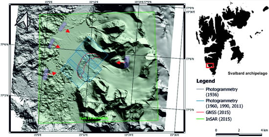
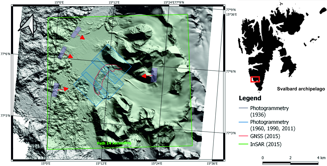
The main goal of this study is to provide a description and an interpretation of changes observed on the surface of the end moraine of the Werenskiold Glacier (Figure 1), which is located in the southwest part of the Spitsbergen [27]. The time span for the analyzed morphological changes was divided into two periods determined by the measurement technique used as the basis for this study. The first, long-term period covers photogrammetry measurements first performed in 1936 and continued until 2011. These were supplemented with the direct survey from 2015. As a result, it was possible to determine changes in the shape of the moraine surface (as well as the changes of the volume of the moraine itself) over a period of 80 years.
In turn, the InSAR technology was used to demonstrate the values of changes over 1 year (and more specifically—for the summer period). It showed (as will be further discussed below) that these changes occur at a fast pace and are impossible to be traced using traditional survey methods (e.g., GNSS). Importantly, photogrammetry is prone to external limitations (such as atmospheric precipitation, clouds, wind), and a GNSS survey is time-dependent: it is prolonged and requires the involvement of a significant number of people. For the above reason, it was impossible to select only one universal method to describe the problem addressed by the authors of this article.
2. Materials and Methods
The long-term changes were analyzed on the basis of numerical terrain models developed from aerial photographs taken in 1936, 1960, 1990, and 2011 for the Polar Norsk Institute in Oslo (cf. Figure S2). These photographs are the only datasets available free of charge for the analyzed area. Low frequency of the photogrammetry missions in the area has been mainly the result of difficult weather conditions. Depending on the date of the photographs, they are either black and white or in color. The photographs are orthogonal, taken with a camera installed under the plane fuselage. The photographs from 1936 are an exception in that they are oblique and taken from the board of the plane (Figure 2a). Figure 2 shows selected images from each of the photogrammetry flights: the black and white photographs of 1936 (Figure 2a) and 1960 (Figure 2b), and the color photographs of 1990 (Figure 2c) and 2011 (Figure 2d). After 2011, due to the high financial costs, photogrammetry flights have not been performed in the analyzed southern Spitsbergen region. The photographs and the prepared photogrammetry materials are characterized in the supplementary material (Table S1).
In the first step, the input data (Table 1) in the form of images were used to develop the Digital Surface Model (DSM) for each analyzed year. The Digital Terrain Model (DTM) was based on data in the form of a point cloud obtained by processing photogrammetric data in the Agisoft computing environment—with the use of Agisoft PhotoScan Professional tools. The height field surface algorithm with the closest neighbor interpolation served to prepare a Triangulated Irregular Network (TIN) from the point cloud. All Digital Terrain Models (DTM) were fitted to the Universal Transverse Mercator (UTM) system, in the 33X zone, on the basis of 7 characteristic points identified in each photograph in each of the measurement periods (the location of these points is presented in Figure S3). The accuracy of the models was within 1–2 m in the case of horizontal components and within 2–3 m for the vertical component.
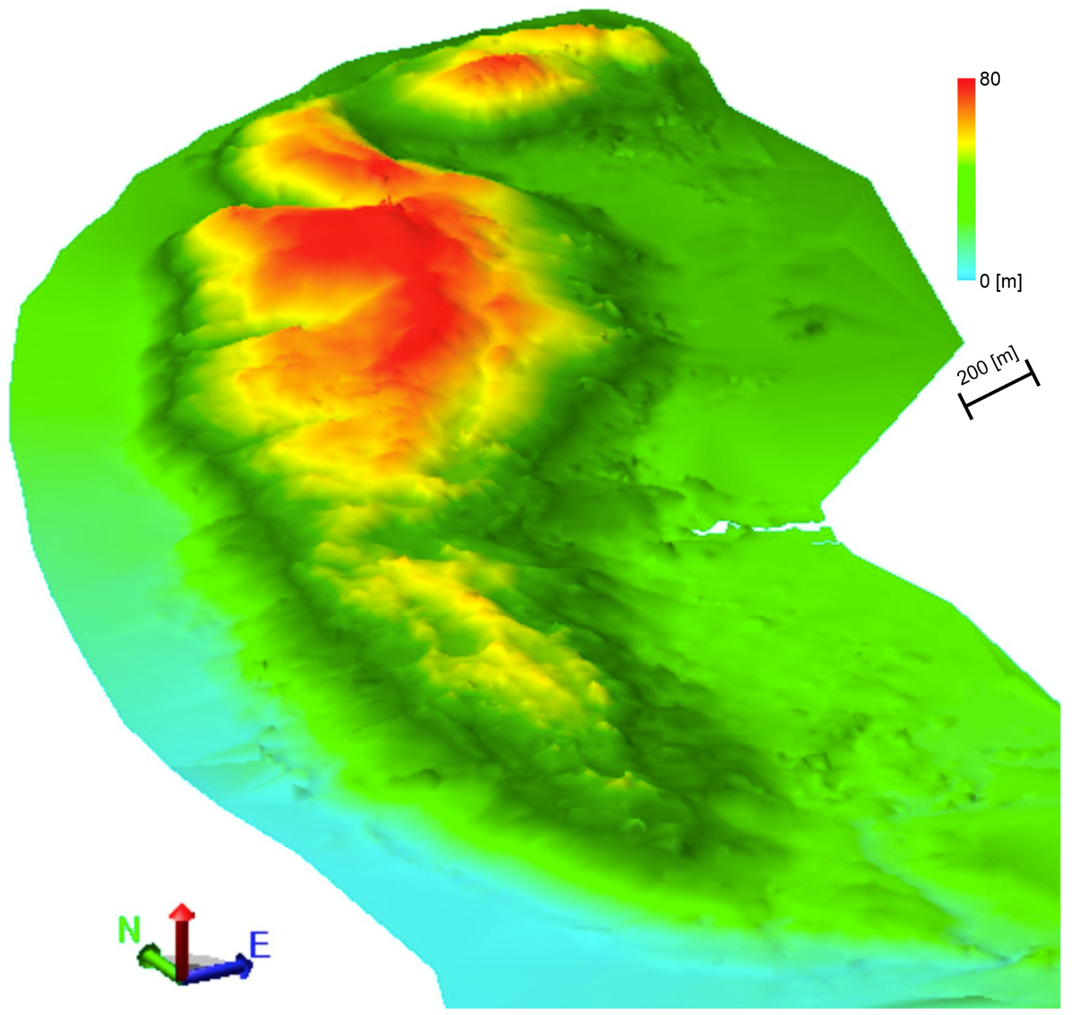
The analyses were also based on the DTM developed from direct in situ surveys of the surface of the end moraine performed in 2015 (Figure 3). The surveys followed the GNSS method and used the reference stations existing in Spitsbergen: NYA1 in Ny-Alesund and ASTRO in the vicinity of Polish Polar Station in Hornsund. It is worth mentioning here that the length of the analyzed area of the end moraine is approximately 3 km, the distance between the measurement points and the closest reference point in Hornsund is approximately 12.1 km, and the distance to the farthest point is 14 km. However, the distance to the second reference point (Ny-Alesund) is above 200 km. Corrections from the reference points were obtained after the measurement, at intervals of 5” and 30” from the closest station, and of 30” from the farthest station. The data was postprocessed and adjusted to the two reference points. The GNSS measurement has the greatest accuracy—with allowance for the corrections from the reference points, and the location accuracy for each of the measurement points was at a level of below ten centimeters (for the horizontal components) and above ten centimeters (for the vertical components). The lowest accuracy obtained for a single point was characterized by horizontal accuracy of ±8 cm and vertical accuracy of ±11 cm as well (this level of accuracy was achieved in the post-processing mode). The highest achieved accuracy of points measured in the GNSS RTK method was ±1.5 cm for the horizontal components and ±2.5 for the vertical component. The survey was performed by 4 people and lasted for 6 weeks, providing a total of 20,721 points.
The short-term changes were analyzed with the use of synthetic aperture radar interferometry (InSAR). The scenes used in the study were acquired from the Sentinel-1A satellite, Single Look Complex (SLC), Path 14, Ascending, Polarization HH, Frequency band C (λ: 5.55 cm), LOS (orientation/incidence angle: 69.5°/37.3°). It allows the terrain surface changes to be traced at practically any time intervals. The only limitation is due to time periods in which the radar images were taken and the availability of the source materials in the European Space Agency (ESA) service or in its mirror services [48,49,50].
The InSAR calculations were performed according to an algorithm, with the use of the GMTSAR algorithm [51]. We co-registered and multi-looked single-look complex (SLC) images using a range/azimuth multi-looking factor of 2.3 × 13.9 m pixel resolution, providing a ground resolution of approximately 40 × 40 m. Simplified locations for the radar scenes are provided in the supplementary material (cf. Figure S2).
Due to a significant diversity of the investigated processes and to the substantial change rate in the end moraine, the interferograms were generated at a maximum base timeline of 24 days, which allowed data coherence and a possibility to determine phase differences [39]. The interferences occur when the displacement speed exceeds one fourth of the wavelength during the time interval. In the case of the prepared interferograms, this is 1.39 cm, i.e., a period of 6–24 days. Spatial base lines were limited to 150 m (details to be found in Figure S1). This study was based on the scenes from 2015. The details of the images are provided in the supplementary material (cf. Table S2). However, the presentation includes only seasonal displacements (June–November). The data series was ended in November, as the winter snowfall causes the images to be decorrelated [52]. The noise level was reduced in all interferograms by employing a spatially adaptive, coherence-dependent Goldstein filter [53,54]. Strongly decorrelated interferograms were removed and not involved in the calculations of the deformations. The impact of the atmospheric layers was mitigated by fitting the linear relationship between the residual phase and the topography [55], using the Digital Elevation Model (DEM) obtained from the GNSS surveys of 2015. Pixels with noise were removed by employing a coherence filter (coherence above 0.3–0.48 for 48% of the interferograms). The interferograms were unwrapped with the use of the Statistical-Cost, Network-Flow Algorithm for Phase Unwrapping (SNAPHU) [56]. The interferograms were corrected by averaging all of the pairs in common images, using Atmospheric Phase Screening (APS) for each scene [57]. All of the InSAR results spatially relate to the first image of August 02, 2015. The implementation of multiple time series reduces the atmospheric effects owing to the assumed temporarily non-correlated tropospheric effects [58,59].
Based on the interferograms, the authors estimated the displacement time series by following the Small Baseline Subset (SBAS) method [39]. The phases were reversed with the use of the cost function based on the L1 standard, in relation to the unwrapping errors [60]. The results for the analysis of the InSAR time series for the data set correspond to single-dimensional (1D) displacement speeds along the LOS (Line Of Sight; details of the analysis are provided in Table S2). On the map, the obtained pixel corresponds to an area of 40 × 40 m.
3. Results
The quality of the developed terrain models varies. The oblique photographs from 1936 allowed the model of the terrain to be precise with respect to altitudes—the fitted photographs advantageously result in a dense point cloud. The effect is satisfactory owing to the use of seven photographs taken from different locations. The pixel resolution, however, is on the order of more than ten meters, and as a result affects the quality of the model. The locations of the photographs are available at [46]. The 1960 model is acceptable, as it shows the differences of both the altitudes and the terrain forms. The point cloud from this model is sufficiently diversified—it is based only on three photographs showing the end moraine of the glacier. The black and white photographs have a very good light exposure and a resolution in the order of more than ten meters, which increases the value of the model. The 1990 model has the worst quality. The point cloud is blurred and “flat”, and does not allow the values of the surface changes to be fully identified. The model is based on three photographs. The images have a very small depth of field—the photographs are in color, but the colors do not reflect the altitude differences. The pixel resolution is in the order of more than ten meters. The 2011 model is probably the worst, despite the quality of the input data used (Figure 4). The reason for this lies in heavy clouds on the day of the measurement, which led to the development of pits and spikes in the model.
The results of the GNSS direct survey are the most accurate and therefore allow the most precise DTM model. This precision results from the possibility to allow for corrections in identifying positions in 3D space provided by the reference points (GNSS permanent stations). The obtained location precision for each of the measurement points is in the order of several centimeters (for the horizontal components) and above ten centimeters (for the vertical component).
The SAR-based analysis of the surface shape of the end moraine indicates very dynamic changes. The surface of the moraine is undergoing constant modifications, with unexpectedly occurring sink holes and scarps, as well as uplifts and banks in their vicinity. The accuracy of the calculated displacements in the quasi-vertical (LOS) plane is ±3 cm (the analysis did not involve changes in the horizontal plane), and the displacements observed on the surface of the end moraine are greater than the measurement errors, suggesting that the employed method was adequate.
4. Discussion
4.1. Long-Term Analysis
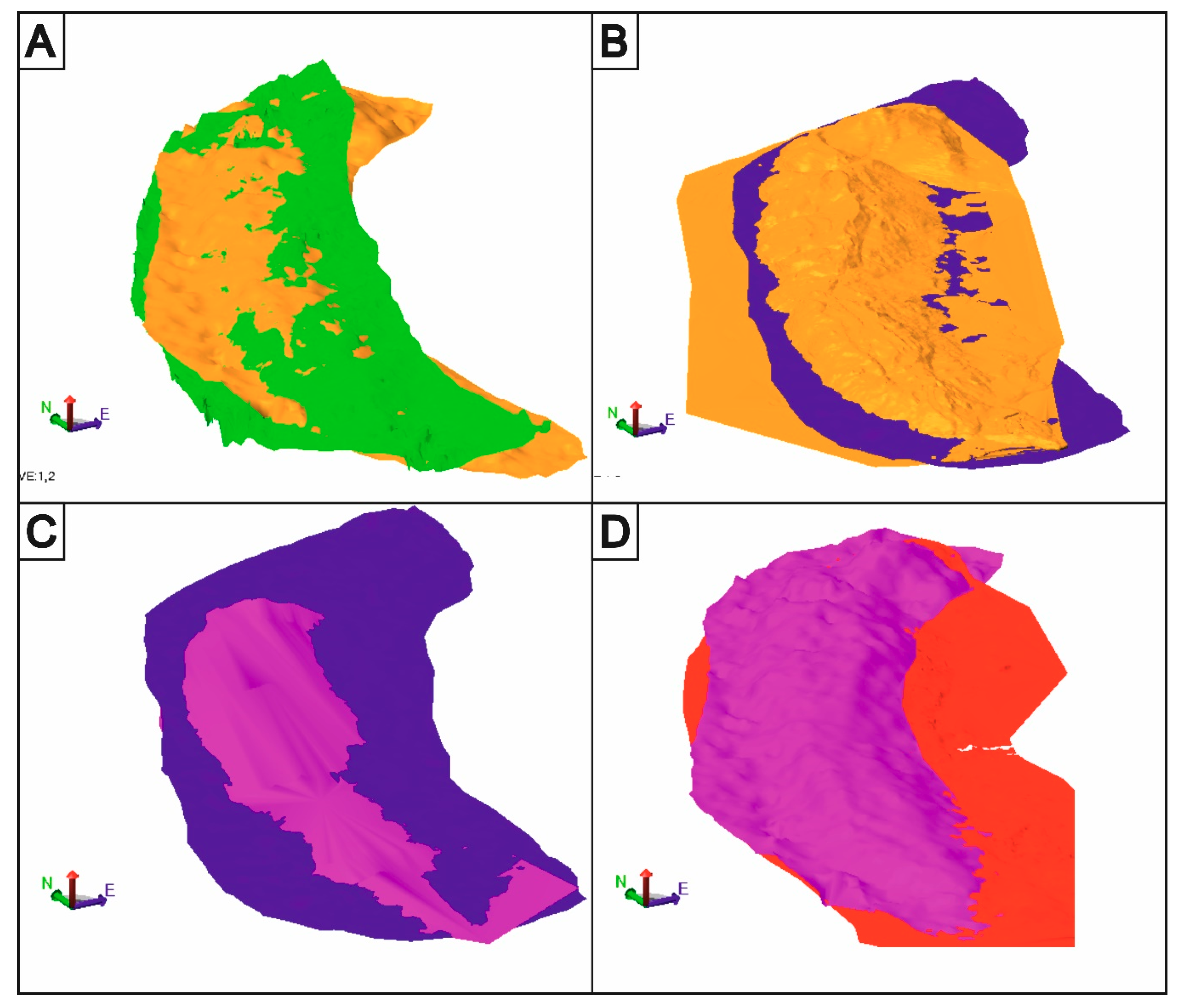
The DTMs prepared on the basis of the photogrammetric data were subjected to a differential analysis for the successive measurement periods. The obtained results allow both the evaluation of the morphological changes, i.e., the changes of the geometry of the end moraine (Figure 5) and the calculation of the volume differences for the entire structure (Table 2).
The greatest volume change occurred between 1960 and 1990. The outflow of the material from the end moraine was at 8.5 million m3, with an inflow of 4 million m3. In the subsequent period, a greater part of the moraine material was accumulated—more than 4.5 million m3. However, this result may not be reliable, and a significant measurement error is possible. The observed precision of the DTM allows a conclusion that the 1990 model has a limited accuracy. Its bias is indicated by the significant changes with respect to both the previous and the following models. The model is flat, which is well visible in the longitudinal cross-section of the overlapped models from individual measurement periods.
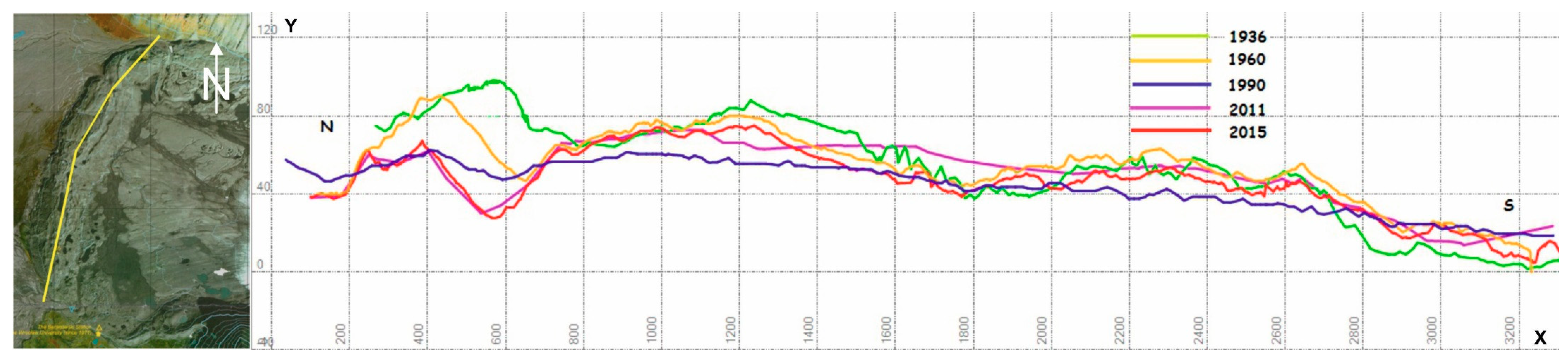
The longitudinal profile is drawn along the entire length of the analyzed object and across each of its surfaces (Figure 6). The graph shows the greatest changes in the northern part of the moraine; it is also visible in the photogrammetric photos attached in the study. The cause is most likely the central moraine, which in the 1940s reached the end moraine. Then the central moraine was completely melted, retreating more than one kilometer along with the glacier, as seen in the photo from 2011. The central moraine is also made of an ice core, and as it melted, it released a large amount of water, which washed out the northern part of the end moraine. The process is visible on the longitudinal profile. In addition, the attached photo from 1936 clearly shows that in the northern part of the moraine there was the highest terrain point, which currently is in the middle part of the moraine.
The morphological changes of the moraine vary. The greatest changes, and this being even despite the limited accuracy of the spatial models, were observed in the northern part of the research area, where the terrain subsidence reaches ~33 m—in its central part the subsidence is ~6 m, and in the southern part it is ~18 m. Over the period of 80 years, a rise visible in the northern part of the moraine was degraded. Additionally, in its northern part, the end moraine was approached by the medial moraine, which is now completely washed, as visible in the photogrammetric images (Figure 2). The total change of the moraine volume between 1936 and 2015, as calculated by comparing the DTMs, reached almost 14 million m3. The washing of the moraine in its northern and southern parts may result from the path of the glacial river bed. Earlier, the bed extended over the northern end of the moraine, whereas presently no glacial river is found in the northern part of the moraine and the bed is completely dry. The glacial river currently extends in the southern part of the moraine and most probably washes it. The end moraine of the glacier is built of the ice core [27,61], and the flowing river has a significant impact on the thawing of the ice, resulting in the degradation of the moraine manifested in its changing geometrical shape.
4.2. Short-Term Analysis
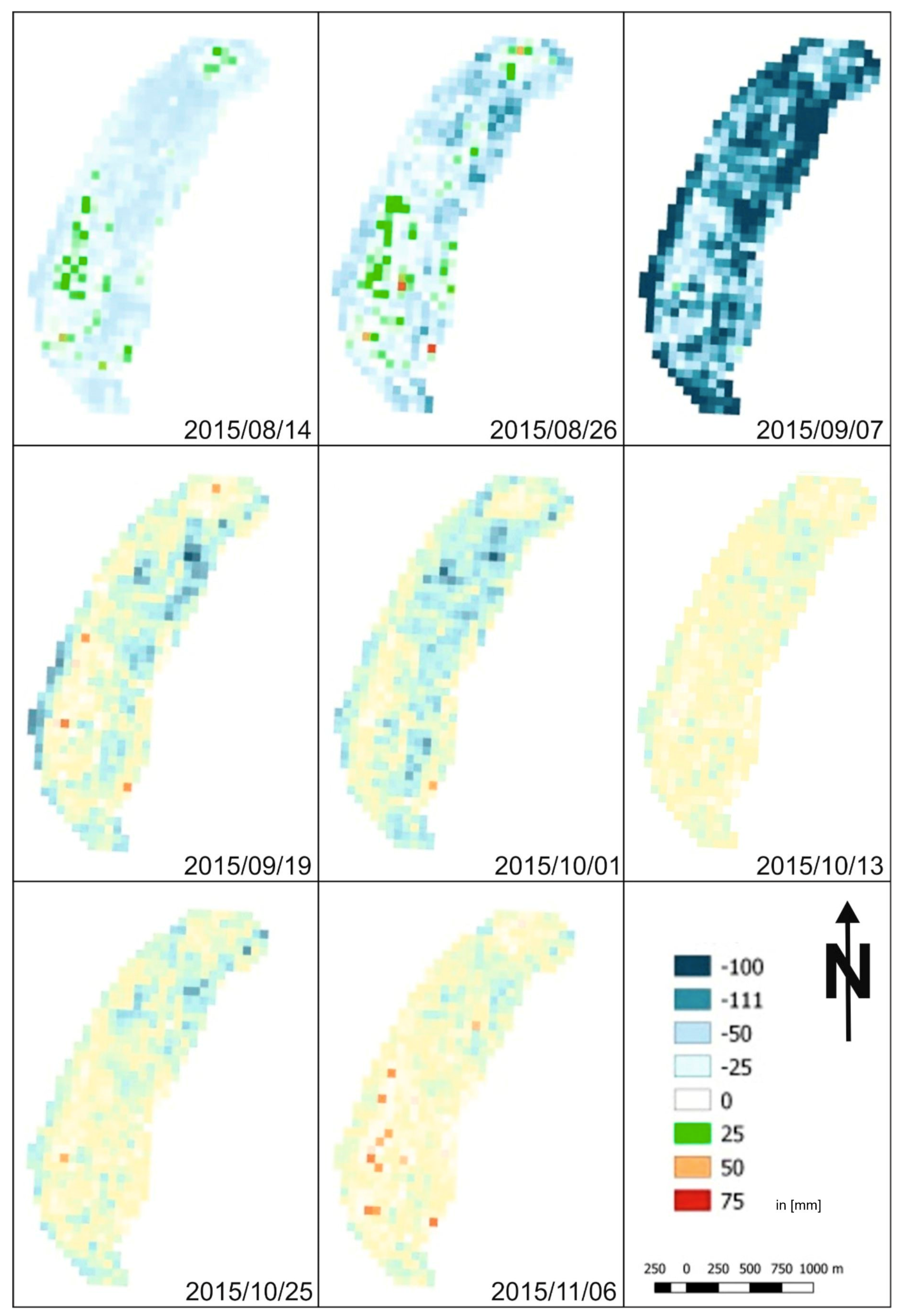
The measurement results and the models constructed on their basis were used to prepare differential analyses. The scene of 2 August, 2015 is the reference image, and each successive image is the difference between the shape of the terrain surface and the reference scene. The deformation models were named in accordance with the image dates. The displacement values are symbolized with the pixel color, on a scale from dark blue in areas of most significant subsidences to dark brown in areas of the greatest rise. Stable areas are represented in white. The LOS displacement values are shown in millimeters (Figure 7).
The above allowed a conclusion that the most significant changes on the surface of the moraine occurred in August and September 2015 (Table 3), which may be related to the atmospheric conditions. The turn of September was a period of the most intensive precipitation over the three analyzed months, as measured in the Hornsund station [25,26], which is located at a distance of 12 km in a straight line from the research area. The least significant changes were identified in September, possibly due to stable weather conditions observed in the area over that period. The total change of the material volume in the moraine reaches 250 thousand m3. The weather variations were not recorded in the research area, and the 12 km distance in a polar region separated by a mountain range may be a source of error and lead to the misinterpretation of the obtained values.
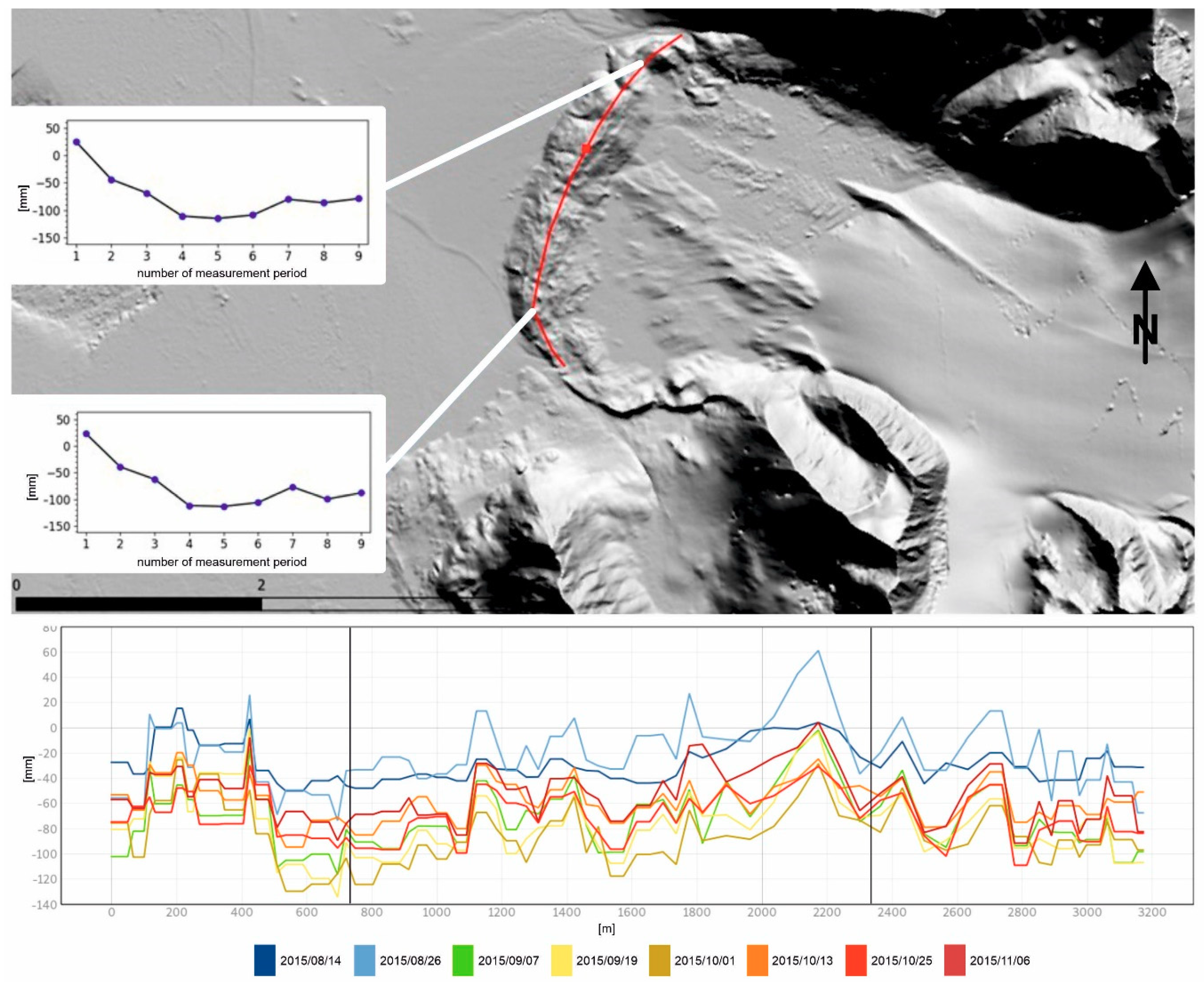
The results of the longitudinal profile analysis allow a conclusion that the entire moraine is subject to a phenomenon of general subsidence, albeit at a varied rate depending on the part of the moraine. The speed of the changes may result from different reasons, such as exposure, thickness of the moraine material cover, the presence of rockfalls, and flows or permanent water reservoirs (e.g., lakes) and waterways in the surface of the moraine. The displacement diagrams for two selected points located within the profile (Figure 8) indicate that the changes in these points reach a value of above 10 cm.
Additionally, an analysis was performed of the obtained results, i.e., the DTMs from satellite images, constructed along the longitudinal profile drawn between the southern and the northern part of the moraine (Figure 8).
4.3. Accuracy of the Results
The accuracy of the results depends largely on the employed measurement method. For research purposes, the accuracy analysis was simplified and limited only to the order of magnitude for the values obtained in the measurements. The main results of this research are the calculated vertical changes of the end moraine surface of the analyzed glacier. The altitude determined on the basis of the photogrammetric images from 1936, 1960, and 2011 remains accurate to 5 m and depends on the size of the pixel and the corresponding terrain unit. The photogrammetry measurement from 1990 is less precise—the altitude is calculated with an accuracy of approximately 10 m. The accuracy of the direct survey from 2015 is in the order of 10 cm and depends on the number of satellites observed during the measurement and on the corrections obtained from the reference stations. If the changes of the surface shape are considered as a difference between two models, then the accuracy of displacement calculations in one point (pixel) is a value of ±7 m in photogrammetry-based methods. For the entire, very diversified, research area (the end moraine), the error value of the calculated difference between the surface models reaches as much as ±300 thousand m3.
In the case of InSAR imaging, this error is in the order of ±30 mm for the calculations of pseudo-vertical (LOS) displacements in which the surface changes are considered as a difference between successive images. The on-surface location of points for which the displacements were calculated depends on their precise identification. The volume calculation error in this case is of ±500 m3.
5. Conclusions
The long-term measurements indicate a tendency and a direction of changes which have occurred on the surface of the end moraine of the Werenskiold Glacier over the last 85 years. The moraine is changing, significantly losing its volume and collapsing inwards without changes on the surface, on which it is located. The most significant changes are observed in its northern part, where the hill located northwards over the medial moraine has undergone an almost complete degradation. The second region affected by the changes is the southern part of the moraine, where large-surface sink holes occur, forming a very diversified landscape.
The short-term changes in the shape of the moraine surface result, among other things, from rockfalls, creep of the erratic material, and favorable ground conditions. This is particularly well visible in the northern and southern parts, where the steep moraine slopes accelerate the process of loose material falling towards the moraine foot. The morphological changes are also influenced by the melting of the ice deposited in the moraine; the so-called ice core of the moraine, which is clearly visible in the form of numerous outflows. The analysis of SAR images enabled the detection of locations in which this process is the most intensive. This would be impossible with the use of traditional measurement methods such as photogrammetry, which is expensive, or direct surveys, which are expensive and time-consuming. Unfortunately, the pixel resolution in InSAR is significantly smaller than in the above traditional methods. During traditional GPS-based measurements over the period of 6 weeks, the moraine changed its volume in a manner both noticeable and measurable with the use of SAR technology. Its deformations reached 10 cm, as illustrated in Figure 8. Unfortunately, the assumed method of GNSS surveys and result processing did not allow a similar standard accuracy level for the GNSS RTK technique during the 2015 measurement session. Photogrammetric images could allow a precise identification of locations most prone to erosion, but the cost related to taking and processing the photographs is very high. In addition, atmospheric conditions frequently prevent photogrammetry flights.
The analysis of both the short-term and the long-term changes allows the identification of the degradation processes in the structure of the moraine. The most significant changes were observed in the northern and southern parts of the moraine, which is most probably related to the changing path of the glacial river bed. The northern part does not have a river, which completely dried in the erosion process. The changes which can be observed in the aerial photographs significantly influence the washing and melting of the ice core in the moraine, especially during the summer period. The InSAR analyses confirm both the locations of the changes and the areas of their greatest dynamics.
The long-term changes are identified with a limited accuracy which depends only on the quality, in this case on the resolution of the aerial photographs, or on the accuracy of direct surveys. The analysis of the short-term changes, illustrated with the use of LOS images, which precisely indicate the areas of deformations, allows the identification of the locations in which the shape of the end moraine surface is most prone to changes. The size of the pixel is not a limitation in this case, as the emphasis is on the location of the area potentially affected by erosion.
Being instantaneous measurement methods, aerial photographs and SAR images enable a quick identification of current surface shape, with the entire moraine represented at the same time. Direct surveys require a long time to be performed (between 5 and 6 weeks). They are also an expensive solution, as is photogrammetry. The SAR technology does not involve any costs (in the case of the Sentinel 1 satellite) and at present is available at 6-day intervals.
Supplementary Materials
The following are available online at https://www.mdpi.com/article/10.3390/rs13112134/s1. Table S1: Photogrammetry parameters, Table S2: InSAR processing methods and parameters, Figure S1: Baseline plot of interferograms generated and selected for dataset, Figure S2: Location of the pictures and measurements, Figure S3: Location of photogrammetry control points.
Author Contributions
Conceptualization, T.G. and D.K.; methodology, T.G. and D.K.; software, T.G.; validation, T.G.; formal analysis, T.G.; investigation, D.K.; resources, T.G.; data curation, T.G.; writing—original draft preparation, T.G. and D.K.; writing—review and editing, D.K.; visualization, D.K.; supervision, T.G. and D.K.; project administration, T.G. and D.K. All authors have read and agreed to the published version of the manuscript.
Funding
This research received no external funding.
Institutional Review Board Statement
Not applicable.
Informed Consent Statement
Not applicable.
Data Availability Statement
The data presented in this study are available on request from the corresponding author. The data are not publicly available due to privacy restrictions.
Conflicts of Interest
The authors declare no conflict of interest. The funders had no role in the design of the study; in the collection, analyses, or interpretation of data; in the writing of the manuscript, or in the decision to publish the results.
References
- Rignot, E.; Koppes, M.N.; Velicogna, I. Rapid submarine melting of the calving faces of West Greenland glaciers. Nat. Geosci. 2010, 3, 187–191. [Google Scholar] [CrossRef]
- Jenkins, A. Convection-Driven Melting near the Grounding Lines of Ice Shelves and Tidewater Glaciers. J. Phys. Oceanogr. 2011, 41, 2279–2294. [Google Scholar] [CrossRef] [Green Version]
- Motyka, R.J.; Dryer, W.P.; Amundson, J.; Truffer, M.; Fahnestock, M. Rapid submarine melting driven by subglacial dis-charge, LeConte Glacier, Alaska. Geophys. Res. Lett. 2013, 40, 5153–5158. [Google Scholar] [CrossRef]
- Carey, M. In the Shadow of Melting Glaciers: Climate Change and Andean Society; Oxford University Press: Oxford, UK, 2010. [Google Scholar]
- Milillo, P.; Rignot, E.; Rizzoli, P.; Scheuchl, B.; Mouginot, J.; Bueso-Bello, J.; Prats-Iraola, P. Heterogeneous retreat and ice melt of Thwaites Glacier, West Antarctica. Sci. Adv. 2019, 5, eaau3433. [Google Scholar] [CrossRef] [Green Version]
- Smith, J.A.; Graham, A.G.C.; Post, A.L.; Hillenbrand, C.-D.; Bart, P.J.; Powell, R.D. The marine geological imprint of Antarctic ice shelves. Nat. Commun. 2019, 10, 1–16. [Google Scholar] [CrossRef] [PubMed] [Green Version]
- Rignot, E.J. Fast Recession of a West Antarctic Glacier. Science 1998, 281, 549–551. [Google Scholar] [CrossRef] [PubMed] [Green Version]
- Rignot, E.; Jacobs, S.; Mouginot, J.; Scheuchl, B. Ice-Shelf Melting Around Antarctica. Science 2013, 341, 266–270. [Google Scholar] [CrossRef] [Green Version]
- Dowdeswell, J.A.; Hagen, J.O.; Björnsson, H.; Glazovsky, A.F.; Harrison, W.D.; Holmlund, P.; Jania, J.; Koerner, R.M.; Lefauconnier, B.; Ommanney, C.S.L.; et al. The Mass Balance of Circum-Arctic Glaciers and Recent Climate Change. Quat. Res. 1997, 48, 1–14. [Google Scholar] [CrossRef] [Green Version]
- Jania, E.; Hagen, E. Mass Balance of Arctic Glaciers; University of Silesia, Faculty of Earth Sciences: Katowice, Poland, 1996. [Google Scholar]
- Gardner, A.S.; Moholdt, G.; Wouters, B.; Wolken, G.J.; Burgess, D.O.; Sharp, M.J.; Cogley, J.G.; Braun, C.; Labine, C. Sharply increased mass loss from glaciers and ice caps in the Canadian Arctic Archipelago. Nature 2011, 473, 357–360. [Google Scholar] [CrossRef]
- Steiner, D.; Pauling, A.; Nussbaumer, S.U.; Nesje, A.; Luterbacher, J.; Wanner, H.; Zumbühl, H.J. Sensitivity of European glaciers to precipitation and temperature—Two case studies. Clim. Chang. 2008, 90, 413–441. [Google Scholar] [CrossRef] [Green Version]
- Haeberli, W.; Noelle, M. Application of inventory data for estimating characteristics of and regional climate-change effects on mountain glaciers: A pilot study with the European Alps. Ann. Glaciol. 1995, 21, 206–212. [Google Scholar] [CrossRef] [Green Version]
- Vincent, C.; Fischer, A.; Mayer, C.; Bauder, A.; Galos, S.P.; Funk, M.; Thibert, E.; Six, D.; Braun, L.; Huss, M. Common climatic signal from glaciers in the European Alps over the last 50 years. Geophys. Res. Lett. 2017, 44, 1376–1383. [Google Scholar] [CrossRef]
- Bolch, T.; Kulkarni, A.; Kääb, A.; Huggel, C.; Paul, F.; Cogley, J.G.; Frey, H.; Kargel, J.S.; Fujita, K.; Scheel, M.; et al. The State and Fate of Himalayan Glaciers. Science 2012, 336, 310–314. [Google Scholar] [CrossRef] [Green Version]
- Fujita, K.; Nuimura, T. Spatially heterogeneous wastage of Himalayan glaciers. Proc. Natl. Acad. Sci. USA 2011, 108, 14011–14014. [Google Scholar] [CrossRef] [PubMed] [Green Version]
- Bolch, T.; Pieczonka, T.; Benn, D.I. Multi-decadal mass loss of glaciers in the Everest area (Nepal Himalaya) derived from stereo imagery. Cryosphere 2011, 5, 349–358. [Google Scholar] [CrossRef] [Green Version]
- Kulkarni, A.V.; Karyakarte, Y. Observed changes in Himalayan glaciers. Curr. Sci. 2014, 106, 237–244. [Google Scholar]
- Davies, B.; Glasser, N. Accelerating shrinkage of Patagonian glaciers from the Little Ice Age (~AD 1870) to 2011. J. Glaciol. 2012, 58, 1063–1084. [Google Scholar] [CrossRef] [Green Version]
- Mark, B.G.; French, A.; Baraer, M.; Carey, M.; Bury, J.; Young, K.R.; Polk, M.H.; Wigmore, O.; Lagos, P.; Crumley, R.; et al. Glacier loss and hydro-social risks in the Peruvian Andes. Glob. Planet. Chang. 2017, 159, 61–76. [Google Scholar] [CrossRef]
- Braun, M.H.; Malz, P.; Sommer, C.; Farías-Barahona, D.; Sauter, T.; Casassa, G.; Soruco, A.; Skvarca, P.; Seehaus, T.C. Constraining glacier elevation and mass changes in South America. Nat. Clim. Chang. 2019, 9, 130–136. [Google Scholar] [CrossRef]
- Cullen, N.J.; Mölg, T.; Kaser, G.; Hussein, K.; Steffen, K.; Hardy, D.R. Kilimanjaro Glaciers: Recent areal extent from satellite data and new interpretation of observed 20th century retreat rates. Geophys. Res. Lett. 2006, 33. [Google Scholar] [CrossRef] [Green Version]
- Moelg, T.; Cullen, N.J.; Hardy, D.R.; Kaser, G.; Nicholson, L.; Prinz, R.; Winkler, M. East African glacier loss and climate change: Corrections to the UNEP article “Africa without ice and snow”. Environ. Dev. 2013, 6, 1–6. [Google Scholar] [CrossRef]
- Prinz, R.; Heller, A.; Ladner, M.; Nicholson, L.I.; Kaser, G. Mapping the Loss of Mt. Kenya’s Glaciers: An Example of the Challenges of Satellite Monitoring of Very Small Glaciers. Geosciences 2018, 8, 174. [Google Scholar] [CrossRef] [Green Version]
- Cisek, M.; Makuch, P.; Petelski, T. Comparison of meteorological conditions in Svalbard fjords: Hornsund and Kongsfjorden. Oceanologia 2017, 59, 413–421. [Google Scholar] [CrossRef]
- Adakudlu, M.; Andersen, J.; Bakke, J.; Beldring, S.; Benestad, R.; Bilt, W.V.; Bogen, J.; Borstad, C.; Breili, K.; Breivik, Ø.; et al. Climate in Svalbard 2100. A Knowledge Base for Climate Adaptation; Norwegian Centre for Climate Services (NCCS): Trondheim, Norway, 2019. [Google Scholar]
- Zwoliński, Z.; Giżejewski, J.; Karczewski, A.; Kasprzak, M.; Lankauf, K.R.; Migoń, P.; Zagórski, P. Geomorphological settings of Polish research areas on Spitsbergen. Landf. Anal. 2013, 22, 125–143. [Google Scholar] [CrossRef]
- Tonkin, T.; Midgley, N.; Cook, S.; Graham, D. Ice-cored moraine degradation mapped and quantified using an unmanned aerial vehicle: A case study from a polythermal glacier in Svalbard. Geomorphology 2016, 258, 1–10. [Google Scholar] [CrossRef] [Green Version]
- Fox, A.J.; Nuttall, A.M. Photogrammetry as A Research Tool for Glaciology. Photogramm. Rec. 1997, 15, 725–737. [Google Scholar] [CrossRef]
- Eiken, T.; Sund, M. Photogrammetric methods applied to Svalbard glaciers: Accuracies and challenges. Polar Res. 2012, 31, 18671. [Google Scholar] [CrossRef]
- Vincent, C.; Wagnon, P.; Shea, J.M.; Immerzeel, W.W.; Kraaijenbrink, P.; Shrestha, D.; Soruco, A.; Arnaud, Y.; Brun, F.; Berthier, E.; et al. Reduced melt on debris-covered glaciers: Investigations from Changri Nup Glacier, Nepal. Cryosphere 2016, 10, 1845–1858. [Google Scholar] [CrossRef] [Green Version]
- Gindraux, S.; Boesch, R.; Farinotti, D. Accuracy Assessment of Digital Surface Models from Unmanned Aerial Vehicles’ Imagery on Glaciers. Remote. Sens. 2017, 9, 186. [Google Scholar] [CrossRef] [Green Version]
- Bindschadler, R.A.; Jezek, K.C.; Crawford, J. Glaciological investigations using the synthetic aperture radar imaging system. Annals Glaciol. 1987, 9, 11–19. [Google Scholar] [CrossRef] [Green Version]
- Rao, Y.S. Synthetic Aperture Radar (SAR) Interferometry for Glacier Movement Studies. Encyclopedia of Snow, Ice and Glaciers; Springer: Dordrecht, The Netherlands, 2011; pp. 1133–1142. [Google Scholar]
- Sharov, A.I.; Osokin, S.A. Controlled interferometric models of glacier changes in south Svalbard. In Proceedings of the Fringe 2005 Workshop, Frascati, Italy, 28 November 2006; pp. 321–365. [Google Scholar]
- Zhou, X.; Chang, N.B.; Li, S. Applications of SAR interferometry in earth and environmental science research. Sensors 2009, 9, 1876–1912. [Google Scholar] [CrossRef] [Green Version]
- Schneevoigt, N.J.; Sund, M.; Bogren, W.; Kääb, A.; Weydahl, D.J. Glacier displacement on Comfortlessbreen, Svalbard, using 2-pass differential SAR interferometry (DInSAR) with a digital elevation model. Polar Rec. 2011, 48, 17–25. [Google Scholar] [CrossRef]
- Liu, G.; Fan, J.H.; Zhao, F.; Mao, K.B. Monitoring elevation change of glaciers on Geladandong Mountain using TanDEM-X SAR interferometry. J. Mt. Sci. 2017, 14, 859–869. [Google Scholar] [CrossRef]
- Rouyet, L.; Lauknes, T.R.; Christiansen, H.H.; Strand, S.M.; Larsen, Y. Seasonal dynamics of a permafrost landscape, Adventdalen, Svalbard, investigated by InSAR. Remote. Sens. Environ. 2019, 231, 111236. [Google Scholar] [CrossRef]
- Johansson, A.M.; Malnes, E.; Gerland, S.; Cristea, A.; Doulgeris, A.P.; Divine, D.V.; Lauknes, T.R. Consistent ice and open water classification combining historical synthetic aperture radar satellite images from ERS-1/2, Envisat ASAR, RA-DARSAT-2 and Sentinel-1A/B. Ann. Glaciol. 2020, 61, 40–50. [Google Scholar] [CrossRef] [Green Version]
- Samsonov, S.; Tiampo, K.; Cassotto, R. Measuring the state and temporal evolution of glaciers using SAR-derived 3D time series of glacier surface flow. Cryosphere Discuss. 2020, 1–21. [Google Scholar] [CrossRef]
- Sommer, C.; Malz, P.; Seehaus, T.C.; Lippl, S.; Zemp, M.; Braun, M.H. Rapid glacier retreat and downwasting throughout the European Alps in the early 21st century. Nat. Commun. 2020, 11, 1–10. [Google Scholar] [CrossRef] [PubMed]
- Ferretti, A.; Prati, C.; Rocca, F. Permanent scatterers in SAR interferometry. IEEE Trans. Geosci. Remote. Sens. 2001, 39, 8–20. [Google Scholar] [CrossRef]
- Berardino, P.; Fornaro, G.; Lanari, R.; Sansosti, E. A new algorithm for surface deformation monitoring based on small baseline differential SAR interferograms. IEEE Trans. Geosci. Remote. Sens. 2002, 40, 2375–2383. [Google Scholar] [CrossRef] [Green Version]
- Hooper, A.; Zebker, H.; Segall, P.; Kampes, B. A new method for measuring deformation on volcanoes and other natural terrains using InSAR persistent scatterers. Geophys. Res. Lett. 2004, 31. [Google Scholar] [CrossRef]
- Interactive Topographic Map of Svalbard Archipelago. Available online: https://toposvalbard.npolar.no/ (accessed on 3 November 2020).
- Official Website of The Norwegian Polar Institute. Available online: https://www.npolar.no/ (accessed on 10 September 2015).
- Ebmeier, S.; Biggs, J.; Mather, T.; Elliott, J.; Wadge, G.; Amelung, F. Measuring large topographic change with InSAR: Lava thicknesses, extrusion rate and subsidence rate at Santiaguito volcano, Guatemala. Earth Planet. Sci. Lett. 2012, 335–336, 216–225. [Google Scholar] [CrossRef] [Green Version]
- Schlögel, R.; Doubre, C.; Malet, J.-P.; Masson, F. Landslide deformation monitoring with ALOS/PALSAR imagery: A D-InSAR geomorphological interpretation method. Geomorphology 2015, 231, 314–330. [Google Scholar] [CrossRef]
- Di Traglia, F.; Nolesini, T.; Ciampalini, A.; Solari, L.; Frodella, W.; Bellotti, F.; Fumagalli, A.; De Rosa, G.; Casagli, N. Tracking morphological changes and slope instability using spaceborne and ground-based SAR data. Geomorphology 2018, 300, 95–112. [Google Scholar] [CrossRef]
- Sandwell, D.T.; Mellors, R.J.; Tong, X.; Wei, M.; Wessel, P. Open radar interferometry software for mapping surface Deformation. EOS 2011, 92, 234. [Google Scholar] [CrossRef] [Green Version]
- Strozzi, T.; Antonova, S.; Günther, F.; Mätzler, E.; Vieira, G.; Wegmüller, U.; Westermann, S.; Bartsch, A. Sentinel-1 SAR inter-ferometry for surface deformation monitoring in low-land permafrost areas. Remote Sens. 2018, 10, 1360. [Google Scholar] [CrossRef] [Green Version]
- Goldstein, R.M.; Werner, C.L. Radar interferogram filtering for geophysical applications. Geophys. Res. Lett. 1998, 25, 4035–4038. [Google Scholar] [CrossRef] [Green Version]
- Baran, I.; Stewart, M.; Kampes, B.; Perski, Z.; Lilly, P. A modification to the Goldstein radar interferogram filter. IEEE Trans. Geosci. Remote. Sens. 2003, 41, 2114–2118. [Google Scholar] [CrossRef] [Green Version]
- Cavalié, O.; Doin, M.-P.; Lasserre, C.; Briole, P. Ground motion measurement in the Lake Mead area, Nevada, by differential synthetic aperture radar interferometry time series analysis: Probing the lithosphere rheological structure. J. Geophys. Res. Space Phys. 2007, 112. [Google Scholar] [CrossRef] [Green Version]
- Chen, C.; Zebker, H. Phase unwrapping for large SAR interferograms: Statistical segmentation and generalized network models. IEEE Trans. Geosci. Remote. Sens. 2002, 40, 1709–1719. [Google Scholar] [CrossRef] [Green Version]
- Tymofyeyeva, E.; Fialko, Y.A. Mitigation of atmospheric phase delays in InSAR data, with application to the eastern California shear zone. J. Geophys. Res. Solid Earth 2015, 120, 5952–5963. [Google Scholar] [CrossRef]
- Lyons, S.; Sandwell, D. Fault creep along the southern San Andreas from interferometric synthetic aperture radar, permanent scatterers, and stacking. J. Geophys. Res. Space Phys. 2003, 108. [Google Scholar] [CrossRef]
- Peltzer, G.; Crampé, F.; Hensley, S.; Rosen, P. Transient strain accumulation and fault interaction in the Eastern California shear zone. Geology 2001, 29, 975–978. [Google Scholar] [CrossRef]
- Lauknes, T.R.; Zebker, H.A.; Larsen, Y. InSAR Deformation Time Series Using an L1-Norm Small-Baseline Approach. IEEE Trans. Geosci. Remote Sens. 2010, 49, 536–546. [Google Scholar] [CrossRef] [Green Version]
- Bennett, M.R.; Huddart, D.; Hambrey, M.J.; Ghienne, J.F. Moraine development at the high-arctic valley glacier Pedersenbreen, Svalbard. Geogr. Ann. Ser. A Phys. Geogr. 1996, 78, 209–222. [Google Scholar] [CrossRef]
Figure 1.
Location of the area of interest: end moraine of the Werenskiold Glacier, SW Spitsbergen (based on [46]).
Figure 1.
Location of the area of interest: end moraine of the Werenskiold Glacier, SW Spitsbergen (based on [46]).

Figure 2.
Examples of source photographs of the Werenskiold Glacier: (A) black and white oblique photograph from 1936; (B) black and white orthogonal photograph from 1960; (C) color orthogonal photograph from 1990; (D) color orthogonal image from 2011 [47].
Figure 2.
Examples of source photographs of the Werenskiold Glacier: (A) black and white oblique photograph from 1936; (B) black and white orthogonal photograph from 1960; (C) color orthogonal photograph from 1990; (D) color orthogonal image from 2011 [47].

Figure 3.
Digital terrain model of the terrain of the glacier end moraine developed from direct surveys in 2015.
Figure 3.
Digital terrain model of the terrain of the glacier end moraine developed from direct surveys in 2015.

Figure 4.
DTMs based on photogrammetric images from different measurement periods: (A) 1936; (B) 1960; (C) 1990; (D) 2011.
Figure 4.
DTMs based on photogrammetric images from different measurement periods: (A) 1936; (B) 1960; (C) 1990; (D) 2011.

Figure 5.
The overlapping DTMs of the end moraine of the Werenskiold Glacier for each of the measurement periods: (A) 1936 (green)–1960 (yellow); (B) 1960 (yellow)–1990 (blue); (C) 1990 (blue)–2011 (purple); (D) 2011 (purple)–2015 (red).
Figure 5.
The overlapping DTMs of the end moraine of the Werenskiold Glacier for each of the measurement periods: (A) 1936 (green)–1960 (yellow); (B) 1960 (yellow)–1990 (blue); (C) 1990 (blue)–2011 (purple); (D) 2011 (purple)–2015 (red).

Figure 6.
Longitudinal profile of the entire length of the moraine and across each of its calculated surfaces. The Y-axis represents elevation variations [m], the X-axis shows the length of the profile [m].
Figure 6.
Longitudinal profile of the entire length of the moraine and across each of its calculated surfaces. The Y-axis represents elevation variations [m], the X-axis shows the length of the profile [m].

Figure 7.
Time series representing the shape changes of the end moraine of the Werenskiold Glacier between 2 August and 6 November, 2015. The first image (upper left) is the reference model.
Figure 7.
Time series representing the shape changes of the end moraine of the Werenskiold Glacier between 2 August and 6 November, 2015. The first image (upper left) is the reference model.

Figure 8.
Longitudinal profile of the InSAR-based DTM displacement locations and values. Locations of points showing the greatest changes over 9 measurement periods.
Figure 8.
Longitudinal profile of the InSAR-based DTM displacement locations and values. Locations of points showing the greatest changes over 9 measurement periods.


Table 1.
Quantitative representation of the data used in long-term analyses.
| Type/Year of Measurement Session | Number of Pictures | Type | Color | Number of Points |
|---|---|---|---|---|
| photogrammetric/1936 | 7 | oblique imagery | black and white | 759 |
| photogrammetric/1960 | 3 | orthoimage | black and white | 1645 |
| photogrammetric/1990 | 3 | orthoimage | color | 5072 |
| photogrammetric/2011 | 6 | orthoimage | color | 3922 * |
* The relatively small number of points results from obstructions in the form of clouds.
Table 2.
Results of the calculated volume differences of the end moraine of the Werenskiold Glacier in each of the analyzed years.
Table 2.
Results of the calculated volume differences of the end moraine of the Werenskiold Glacier in each of the analyzed years.
| Model Data | Volume Loss | Volume Increase | Volume Difference [Absolute Value] | Total Difference |
|---|---|---|---|---|
| [m3] | ||||
| 1936 * | - | - | - | - |
| 1960 | 4,600,000 | 220,000 | 4,380,000 | 4,380,000 |
| 1990 | 8,690,000 | 4,170,000 | 4,520,000 | 8,900,000 |
| 2011 | 1,300,000 | 4,500,000 | 3,200,000 | 12,100,000 |
| 2015 | 2,505,587 | 139,386 | 2,066,201 | 14,166,201 |
* The data for 1936 should be used as reference data.
Table 3.
Volume changes of the end moraine of the Werenskiold Glacier, based on SAR data.
| Model Number (Data of Exposition) | Volume Loss | Volume Increase | Volume Difference [Absolute Value] | Total Difference |
|---|---|---|---|---|
| [m3] | ||||
| 2015/08/02 * | - | - | - | - |
| 2015/08/14 | 49,500.5 | 1540.6 | 47,960.0 | 47,960.0 |
| 2015/08/26 | 13,168.9 | 11,388.4 | 1780.5 | 49,740.5 |
| 2015/09/07 | 85,869.8 | 0.6 | 85,869.2 | 135,609.7 |
| 2015/09/19 | 10,550.4 | 7856.8 | 2693.6 | 138,303.3 |
| 2015/10/01 | 21,535.4 | 6293.9 | 15,241.5 | 153,544.8 |
| 2015/10/13 | 226.3 | 49,165.1 | 48,938.8 | 202,483.6 |
| 2015/10/25 | 23,769.2 | 1393.8 | 22,375.4 | 224,859.0 |
| 2015/11/06 | 684.3 | 29,267.1 | 28,582.8 | 253,441.8 |
* The data from August 2, 2015 should be used as reference data.
Publisher’s Note: MDPI stays neutral with regard to jurisdictional claims in published maps and institutional affiliations. |
© 2021 by the authors. Licensee MDPI, Basel, Switzerland. This article is an open access article distributed under the terms and conditions of the Creative Commons Attribution (CC BY) license (https://creativecommons.org/licenses/by/4.0/).
Share and Cite
MDPI and ACS Style
Głowacki, T.; Kasza, D. Assessment of Morphology Changes of the End Moraine of the Werenskiold Glacier (SW Spitsbergen) Using Active and Passive Remote Sensing Techniques. Remote Sens. 2021, 13, 2134. https://doi.org/10.3390/rs13112134
AMA Style
Głowacki T, Kasza D. Assessment of Morphology Changes of the End Moraine of the Werenskiold Glacier (SW Spitsbergen) Using Active and Passive Remote Sensing Techniques. Remote Sensing. 2021; 13(11):2134. https://doi.org/10.3390/rs13112134
Chicago/Turabian StyleGłowacki, Tadeusz, and Damian Kasza. 2021. "Assessment of Morphology Changes of the End Moraine of the Werenskiold Glacier (SW Spitsbergen) Using Active and Passive Remote Sensing Techniques" Remote Sensing 13, no. 11: 2134. https://doi.org/10.3390/rs13112134
Note that from the first issue of 2016, this journal uses article numbers instead of page numbers. See further details here.