1. Introduction
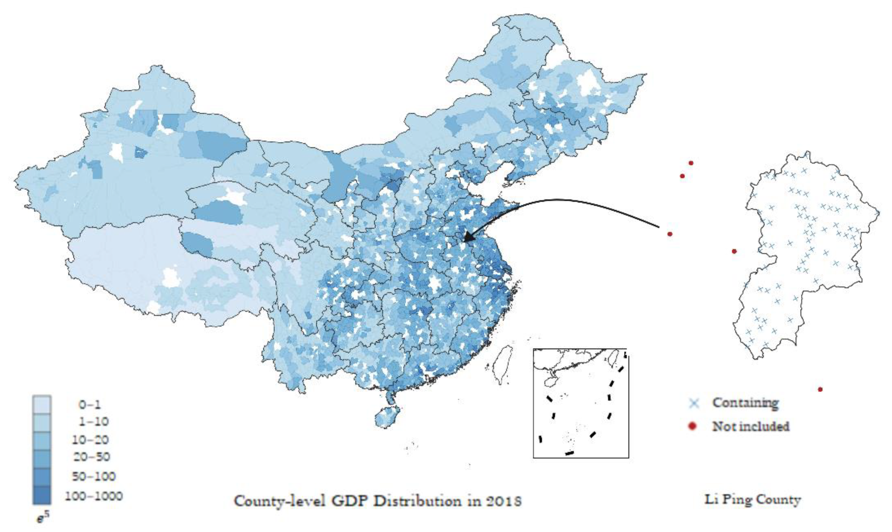
Fine-grained, large-scale measures of economic development levels are vital to resource allocation and policy-making. Gross domestic product (GDP in short) is an elementary but crucial indicator in assessing regional productivity and consumption degrees. Disaggregated GDP maps can reflect both the overall development levels and the regional imbalance within a country. It is worth to emphasize that the geographic administrative hierarchy in China is province, city and county in descending order, county is a relatively small administrative unitwhich is quite different with the system of many other countries. In the Chinese Mainland, the official county-level GDP, i.e., GDP of the second sub-national administrative unit in China [
1,
2], are collected by local government statistical services. The final GDP values are calculated mainly from administrative reporting data and supplemented (or amended) by periodical surveys and censuses. However, official county-level GDP values are often heterogeneous and costly [
3] because statistical institutions at the county level commonly suffer from the lack of specialized persons and the inaccessibility to essential materials [
4,
5].
In recent years, remote sensing data have been increasingly applied to predict socioeconomic indicators [
6]. A series of studies have been conducted to develop convenient and scalable methods to estimating various indices relying on nighttime lights, satellite imagery, and emerging machine learning models. Previous studies have demonstrated the correlation between lit areas and GDP values [
7,
8]. Researchers successfully applied nightlight data and regression methods to generate disaggregated maps of socioeconomic indicators in different regions around the world, including both developed countries such as European Union countries, the United States [
8], and Japan [
9], and developing countries such as India [
10,
11] and China [
12]. However, nightlight data are easily affected by coarse resolution, noise, and oversaturation [
13,
14]. They also overlook the relationship between economic developments and geographic patterns. The rapid development of convolutional neural networks and the availability of high-resolution daytime satellite imagery enable the detection of detailed land appearances thought to be strongly correlated with socioeconomic statuses, such as buildings, cars, roads, and farmlands [
15,
16]. Despite the informativity of daytime satellite imagery, it is often infeasible to estimate socioeconomic indicators directly from daytime images since there are hardly enough ground-truth data to supervise the training of data-intensive CNN-based models. Learned from previous studies, some researchers creatively combined daytime and nighttime remote sensing data [
17,
18]. They regarded nightlight intensities as a data-rich proxy of economic development degrees and applied CNN-based classifiers to predict nightlight from the corresponding daytime images. Later, the high-dimensional output features at a specific layer of CNNs are fed into simple regressors to estimate indicators in interest. In this way, fine-grained GDP maps can be generated conveniently from easily accessed data.
This paper is interested in predicting annual county-level gross domestic product (GDP) around the Chinese Mainland from readily accessed remote sensing data, including daytime satellite imagery and nighttime lights. Our framework is mainly based on the work of Jean et al. [
18], in which paired daytime images and nightlight intensities are utilized for training a CNN classifier, and the output features at a specific layer, after dimensional reduction and statistics calculation, are fed into a simple regressor for the final estimation. We boost the model performance via incorporating attention mechanism into the CNN architecture. To the best of our knowledge, this is the first time that the CNN-based estimation of county-level socioeconomic indicators from remote sensing data have been applied on such a large scale in China, i.e., all over the country. Since the number of image grids belonging to a county-level administrative region varies, each economic index, i.e., annual county-level GDP, corresponds with an indeterminate number of output feature vectors. To uniform the dimensions of downstream model inputs, feature vectors belonging to the same county are regarded as a sample, and the representative statistics are computed as the final independent variables for the regression models.
Our work has the following contributions.
Creativity: To the best of our knowledge, it is the first time that county-level GDP around the Chinese Mainland have been estimated from both daytime satellite imagery and nightlight data using CNNs. Thanks to the scalability of remote sensing data, the proposed model can generate fine-grained estimation maps covering the whole country in a convenient and economical manner;
Convenience: All the daytime satellite images and nightlight intensities fed into the model come from easily accessed, open-source online interfaces. Meanwhile, since the data-rich nighttime lights are applied to supervise the training process, there is also no need to manually annotate the daytime images to ensure the CNN architecture to converge;
Refinement: We modify the CNN classifier by incorporating attention mechanism and achieve better performance;
Robustness: In our framework, all the grid images belonging to the same county are utilized to generate corresponding features. Thus, predicted values are less likely to vary with noise or missing data.
2. Related Work
2.1. Estimating GDP with Nightlight Only
Large amounts of previous studies have investigated the association between economic activities and nighttime lights at different scales and in different areas. The Defense Meteorological Satellite Program (DMSP) and the Visible Infrared Imaging Radiometer Suite (VIIRS) are two main sources of nightlight data applied in socioeconomic research [
19]. The DMSP annual stable lights from 1992 to 2013 published by the NOAA Earth Observation Group (EOG) boosted studies that estimated socioeconomic indicators, GDP for instance, by nighttime luminous data in the last decades. Elvidge et al. [
20] examined the relationship between the area of lighting measured from the DMSP data and country-level GDP for 200 nations. Doll et al. [
7] moved one step further and produced the first-ever global map of GDP using the total lit area of a country, indicating a high correlation between nightlights and GDP at the country level. As fine-grained socioeconomic data became increasingly desirable, the following studies tended to examine the relationship between nightlight and economic activity degrees at smaller geographic units. Doll et al. [
8] successfully produced disaggregated maps for 11 European countries along with the United States at a 5 km spatial resolution using nighttime radiance data and the prevailing land-use data. There also existed evidence that nightlight could be applied to predict sub-national GDP or income levels in developing countries such as India [
10,
11] and China [
12,
21]. These studies verified the rationality of considering nighttime lights (provided by the DMSP data) as a proxy of regional economic activity degrees. However, flaws in DMSP data, including pervasion blurring, no calibration, coarse spatial and spectral resolution, and inter-satellite differences [
14,
22], inflicted inaccuracy and even invalidity upon studies using this data source, especially for smaller units and lower density areas [
23,
24]. In comparison, the new-generation VIIRS data, which became available from 2012 onward, were more pertinent to the needs of socioeconomic researchers. Empirical results proved that the VIIRS data could be a promising supplementary source for socioeconomic indicator measures [
25,
26,
27] and have better performance than the DMSP data [
23,
28].
It should be noticed that despite the superiority to DMSP data, estimation at small geographic units and detection of agricultural activities remained to be challenges for the utilization of VIIRS data [
23,
26]. The estimation of county-level GDP in China from nightlight was only affected by the limitation of data sources. To the best of our knowledge, no studies have ever generated county-level GDP maps covering the whole country. Moreover, many studies either eliminated the output of primary industry, i.e., agricultural output, from local GDP [
29] or incorporated additional information such as land-use status and rural population [
30]. Data that are both informative for small or low-density regions and easily accessed are needed.
2.2. Detection of Economic-Related Visual Patterns from Daytime Satellite Imagery via Deep Learning
Remote sensing data are valuable for economic studies because they provide access to information hard to obtain by other means and generally cover broad geographic areas [
6]. Apart from nighttime lights, daytime satellite imagery is another valuable resource for socioeconomic research. Compared with relatively low-resolution nightlight data, daytime images contain much more features and can reveal more detailed topographic information [
6]. Land appearance detection relying on CNN-based architectures from daytime satellite imagery perform well in locating regions that strongly related to socioeconomic status [
15,
31,
32]. Engstrom et al. [
15] trained CNNs to extract features concerning buildings, cars, roads, farmlands, and roof materials from high-resolution daytime images. They fed these features into a simple linear model and explained nearly sixty percent of both poverty headcount rates and average log consumption at the village level in Sri Lanka. Abitbol and Karsai [
32] applied a CNN model to predict inhabited tiles’ socioeconomic status and projected the class discriminative activation maps onto the original images, interpreting the estimation of wealth in terms of urban topology. To date, daytime imagery and deep neural networks have been widely applied to predict various socioeconomic indicators such as population [
33,
34,
35], poverty distribution [
15,
18,
36], and urbanization [
6,
37]. Despite the convenience and scalability, these studies depend largely on data-intensive CNNs and require large volumes of ground-truth labels to supervise the training process. Han et al. [
6] developed a framework for learning generic spatial representations in a semi-supervised manner. They constructed a small custom dataset in which daytime satellite images were classified into three urbanization degrees by four annotators and applied it to fine-tune the CNN-based classifier pre-trained on ImageNet [
38]. The output features can be adopted to predict various socioeconomic indicators, but the training labels of this method suffered from high expenses and subjective judgments.
2.3. Nightlight as an Intermediate between Economic Indicators and Daytime Satellite Imagery
In many developing countries, reliable sub-regional socioeconomic data are scarce and expensive, making it difficult for data-intensive neural networks to directly learn relevant features from informative daytime satellite imagery. Since nightlight data are much more abundant and commonly correlated with degrees of economic activities, some researchers began to regard them as a data-rich intermediate between economic indicators and daytime satellite imagery. Xie et al. [
17] proposed a two-step transfer learning framework in which a fully convolutional CNN model pre-trained on ImageNet [
38,
39] was tuned to predict nightlight intensities from daytime images and learn poverty-related features simultaneously. They found that the model learned to identify semantically meaningful features such as urban areas, roads, and farmlands from daytime images without direct supervision of poverty indices but with only nighttime lights as a proxy. Jean et al. [
18] refined this method by feeding the features learned from raw daytime satellite imagery by the tuned CNN into ridge regression models to estimate average household wealth in five low-income African countries. Their research further demonstrated that nightlight data could well serve as an intermediate between daytime satellite imagery and socioeconomic indicators relying on deep learning techniques [
40]. Follow-up studies showed that the fully convolutional network, which was tuned to extract high-dimensional features from daytime images under the supervision of corresponding nightlight intensities, could be substituted for various architectures [
40], including DenseNet [
41] and ResNet [
42], and this approach also generalized well to predict poverty-related indices in other countries outside Africa [
43]. Nighttime lights also proved useful when there was a lack of ground-truth socioeconomic data, guiding the CNN-based model to compute economic scores from daytime imagery in an unsupervised way [
18]. Instead of utilizing luminous data as approximate labels to train neural networks, Yeh et al. [
44] trained identical ResNet18 [
42] architectures on daytime and nighttime images, respectively, and then fed the concatenated output features into a ridge regressor to predict cluster-level asset wealth. Although this approach could predict economic indicators from remote sensing data in an end-to-end manner, it required much more efforts processing and matching daytime and nighttime imagery, and would be unable to generate valid estimations when the ground-truth socioeconomic data are insufficient for the CNNs to converge.
3. Data
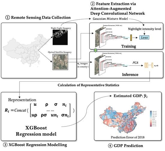
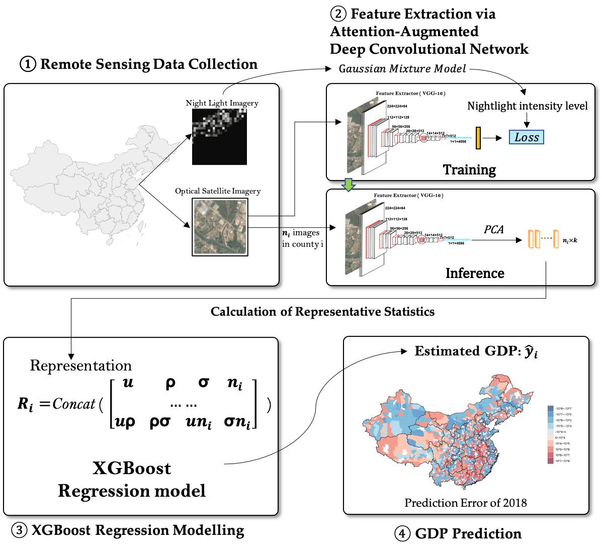
This paper utilizes the following three data sources: daytime satellite imagery, nighttime light maps, and county-level GDP around the Chinese Mainland along with the corresponding administrative boundaries. All the data sources mentioned above are joined together to construct a complete dataset. The brief procedures of collecting and matching data are shown in
Figure 1.
3.1. Daytime Satellite Imagery
We scratch daytime satellite images mainly through an API provided by the Planet satellite. Posting a request consisting of locations and dates in a month-year mode, the API will return a corresponding image of 256 × 256 pixels. In detail, the specific product we utilize is PlanetScope Ortho Scene product (PSScene3Band), where the distortions caused by terrain have been removed.
Each daytime image covers approximately 1 km
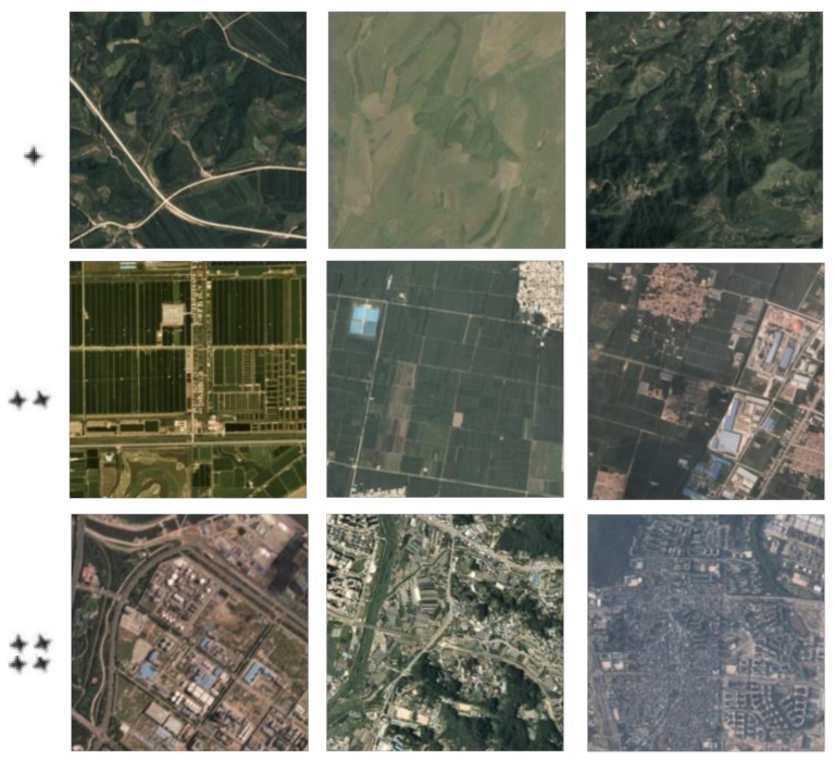
2 with a 5 m resolution, which generally enables human activities to be observed. The natural idea is that we traverse the Chinese Mainland at a 1 km interval so that all the images together can cover the whole territory. However, such a procedure will result in large amounts of images, leading to high time cost in scratching images and over-head computation in training models. As a compromise, we set an interval of 2 km. In this way, the total amount of images is reduced by 4 times, which will greatly speed up for the whole framework. We collect daytime satellite images from 2016 to 2020 according to the grid coordinates. Since the Planet product update image products monthly, the images we scratch are in month granularity of the middle of the year, mostly in June and July. Several instances of daytime satellite imagery are shown in
Figure 2.
3.2. Nighttime Light Maps
As the pioneer of the nocturnal remote sensing technology, the Earth Observation Group (EOG) has been collecting nighttime remote sensing data for years, producing high-quality global nighttime light maps. We utilize the newest V1 annual composites made with the “vcm” version of the year 2016, which covers the Asian area. In this version, the influence of stray light has been excluded. Meanwhile, ephemeral lights and backgrounds (non-lights) are screened out to ensure the ground truth.
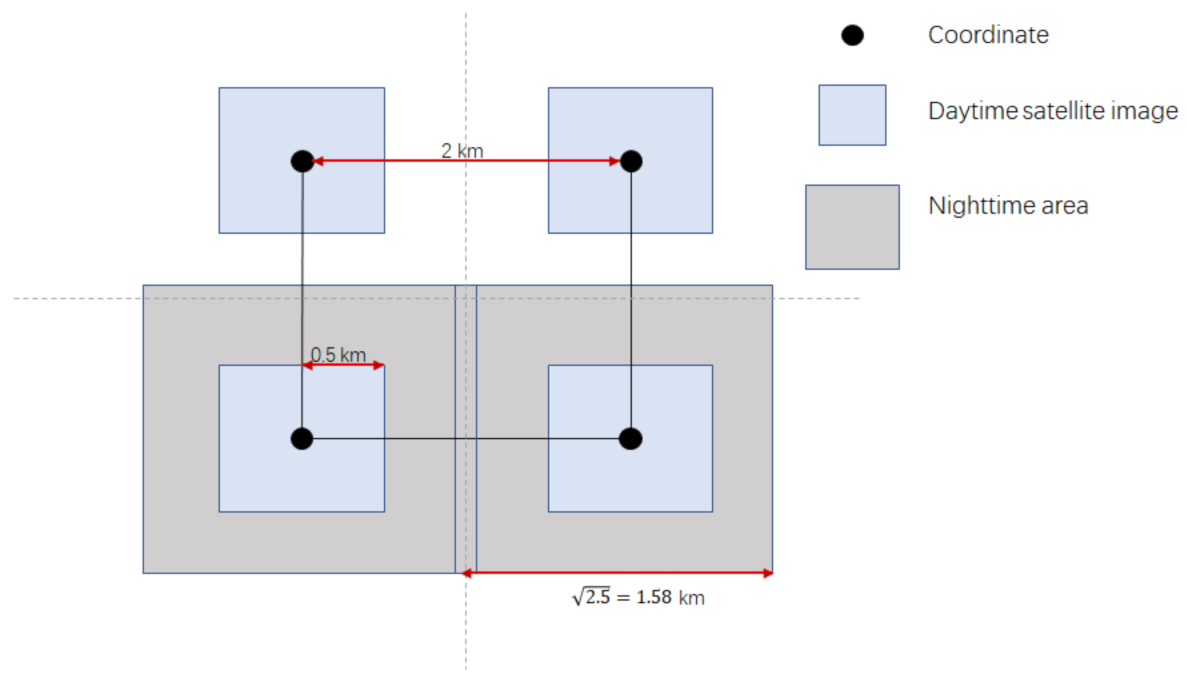
The nighttime light map is then applied to construct labels for daytime satellite imagery. For each daytime satellite image in 2016, we delineate a 2.5 km
2 area centered on the same coordinate and sum up nightlight intensities within the area. The areas we select are slightly larger than daytime images and thus can roughly cover the gaps among those images. We regard the sum of nightlight intensities within each area as a proxy of the economic activity degree for the corresponding daytime satellite image. In addition, we apply the Gaussian mixture model (GMM) to cluster the nighttime light intensities. The Gaussian mixture model is a probabilistic model for representing normally distributed subpopulations within an overall population [
45]. It is a popular clustering algorithm considered as an improvement over k-means clustering. With the GMM clustering method, we divide the nighttime light intensities into three levels: low, medium, and high. Since the proportion of low-level samples is too high, we drop a few samples with low nightlight intensity levels to maintain the data balance. The final distribution of nightlight intensity levels is shown in
Table 1.
3.3. County-Level GDP and County Boundaries
By default, the word “county” in this paper denotes the second sub-national administrative unit in China. County-level units can be mainly divided into three types: municipal districts, counties, county-level cities. Some county-level units, municipal districts for instance, have merged to form larger administrative regions named cities or prefectures, while others are governed directly by the first sub-national units in China, i.e., provinces.
Complex administrative hierarchy makes it difficult to collect annual county-level GDP around the Chinese Mainland from a single publication. This paper sorts to the China Economic and Social Development Statistics Database provided by China National Knowledge Infrastructure (CNKI), where over 28,000 statistical yearbooks concerning different themes released by official statistical institutions at different levels are available. Most annual county-level GDP data can be fetched from the corresponding Provincial Statistical Yearbooks, while a few are supplemented by the Municipal Statistical Yearbooks and the data retrieval function supported by CNKI. In this paper, the annual county-level GDP is measured in ten thousand Chinese Yuan.
The geographic boundary information of county-level units around China is gathered from the National Catalogue Service for Geographic Information (
https://www.webmap.cn, accessec on 14 October 2021). We collected the boundary coordinates of 2900 county-level administrative units along with county names and the names of the cities or provinces these counties are governed by. GDP values are attached to geographic information via names of counties as well as names of the superior administrative units.
In the data matching process, we utilized the geofencing algorithm supported by the Python package geopandas [
46] to compare image coordinates and county boundaries. Specifically, an image along with its nightlight intensity level will be matched with a county once its center falls into the target county-level administrative unit.
Figure 3 shows this matching process.
4. Method
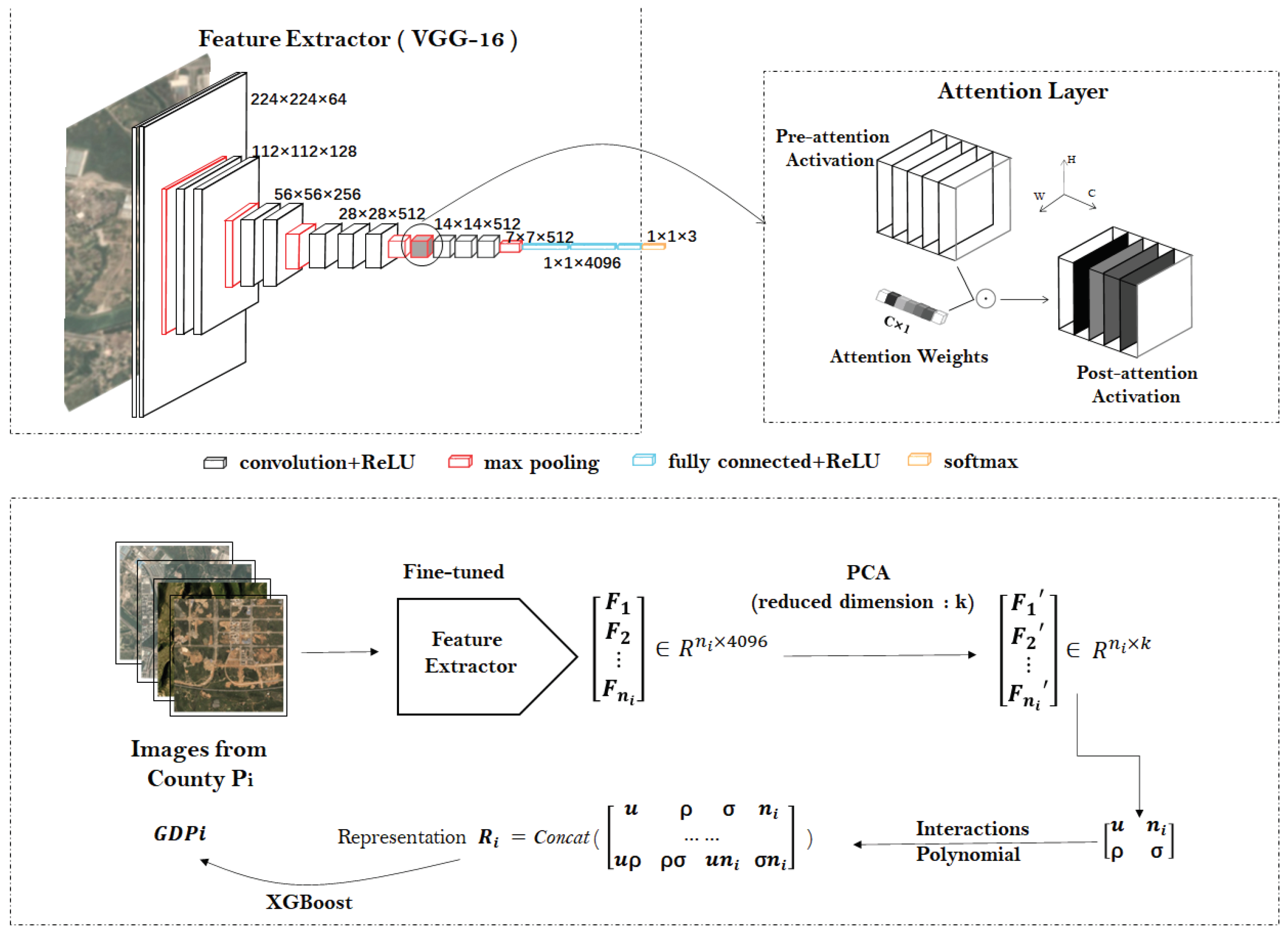
Our target is to predict the annual county-level GDP from daytime satellite imagery and nightlight intensities. Since county-level units in China vary in shape and size, the corresponding amount of satellite images along with nightlight intensity levels are variable. Therefore, it is necessary to uniform input dimensions before estimating GDP values. In our model, we first build an attention-augmented feature extractor under the supervision of paired daytime satellite images and nightlight intensity levels. Given a county i in the whole county set C along with the corresponding daytime satellite image set that contains images, each image such as the j-th image in will be passed through a trained feature extractor to get the economic-related features , , the length of the output vector in the feature extractor. After dimensional reduction, the representative statistical characteristics, including mean, variance, correlation, and the number of each county’s reduced features, are calculated and combined as a fixed-size representation where s is the amount of final used variables. Finally, the representation is fed into a regression model to predict the GDP value at each county.
4.1. Training Feature Extractor via Supervised Learning and Transfer Learning
The attention-based VGG-16 network architecture is utilized to extract features from satellite imagery. The VGG-16 [
47] pre-trained on ImageNet [
38] contains five convolutional blocks, and each block consists of a series of convolution layers, pooling layers, and non-linear activation functions. The convolutional blocks are trained to extract and construct complex features from raw input daytime images. The last two layers of the network are fully connected layers trained to sort stimuli into 1000 predefined categories based on features extracted from the preceding structure. This paper classifies nightlight intensities into three categories, i.e., nightlight intensity levels, and applies them to supervise the training of the extractor. In the last two convolutional blocks of VGG-16, we insert an attention layer that can re-weight the activation representations. Suppose the convolutional block of VGG outputs an activation features
defined as pre-attention activation, the attention layer
matches it in the channel dimension
C correspondingly. Later, the post-attention activation
is calculated as the hadamard product between
and
A:
where
.
The post-attention activation modulated by the attention layer maintains the same shape as the pre-attention activation, and they are then passed into the next block as
Figure 4 shows. We use the Adam optimizer to train the network. The loss function is defined as follows:
where
denotes the ground-truth class probability (i.e., low level, medium level, and high level) and
denotes the predicted probability. When the model converges, we remove the last fully connected layer and utilize the remaining structure to extract features
from satellite imagery.
n, the length of
F, is equal to the length of the output activation flattened by the last convolutional block in VGG-16.
4.2. Dimension Reduction
Once features have been extracted from each satellite image, we intend to reduce the dimension of
F into a smaller size. Since the number of counties applied in this paper of a single year is around 2000, and we aim to utilize the statistical characteristics of a county’s image set to fit GDP values, the dimension is supposed to be less than the number of counties to avoid overfitting. Therefore, we implemented the principal component analysis (PCA) [
48] to reduce the dimensions of the feature
F.
PCA is nonparametric and does not require a parameter tuning process. It applies orthogonal linear transformations of the original vectors to extract principal components with the maximum variance. A sufficient number of principal components should explain most of the variance of the original data and efficiently reducing dimensions. Empirically, the first six components can explain approximately 80 percent of the variance, and additional gains will rapidly become marginal. This paper considers up to the first 25 principal components in the dimension reduction process, i.e., k (3 ≤ k ≤ 25).
4.3. Statistical Characteristics
To address the varying number of daytime images along with nightlight intensity levels belonging to a county, we calculate the statistical characteristics of each image set. In this way, each county has a fixed-sized representation. Following the approach of [
18], we consider the following base statistical characteristics: (1) sample amount
n, i.e., the number of satellite images within a county; (2) the sample mean
; (3) the standard deviation
; and (4) Pearson’s correlation of the reduced features
. These four statistical characteristics are fundamental statistics that can capture the vital traits of an image set. Concretely speaking, these descriptive statistical characteristics represent a sample set through central tendency (the sample mean), dispersion (the standard deviation), association (the correlation), and volume (the sample size). To enrich the independent variable, we apply the feature interaction process in which the interactions and polynomial combinations of features are added. Therefore, the augmented search space can be considered. Finally, for each county
i, we obtain a representation
of the same length
s. The representation is later fed into a regressor to estimate the target county-level GDP.
5. Experimental Results
5.1. Performance Evaluation
In this study, the experiment was conducted in the environment of Public Computing Cloud, Renmin University of China.We applied several methods to evaluate the model performance. Unanimously, we take the data of 2017 as the training set and the data of 2018 as the testing set. K-fold cross-validation is utilized to determine the optimal hyperparameters for PCA and the regression process. The
nightlight method takes the sum of nightlight intensities of each county as the independent variable and applies it to predict the corresponding county-level GDP directly via a regressor. The
no-proxy method utilizes the same VGG-16 architecture as the feature extractor in the proposed framework but only pre-trains it on the ImageNet. The
VAE (variational auto-encoder) method plays the role of feature extractor in our model. A variational auto-encoder [
49] is an unsupervised deep learning algorithm that aims to learn a compressed representation of the input data and recover, limiting the hidden layer’s scale. The
VGG-A denotes our proposed model, which features the attention-augmented VGG network.
As
Table 2 shows, VGG-A (our proposed framework) outperforms all the other methods with an R-squared of 0.71. The satellite imagery does provide abundant features for predicting GDP since the R-squared of only using nightlight intensities is 0.36. Moreover, due to increased predicting quality against no-proxy (0.22) and VAE (0.45), we suggest that using nighttime light as a proxy helps extract more economic-related features.
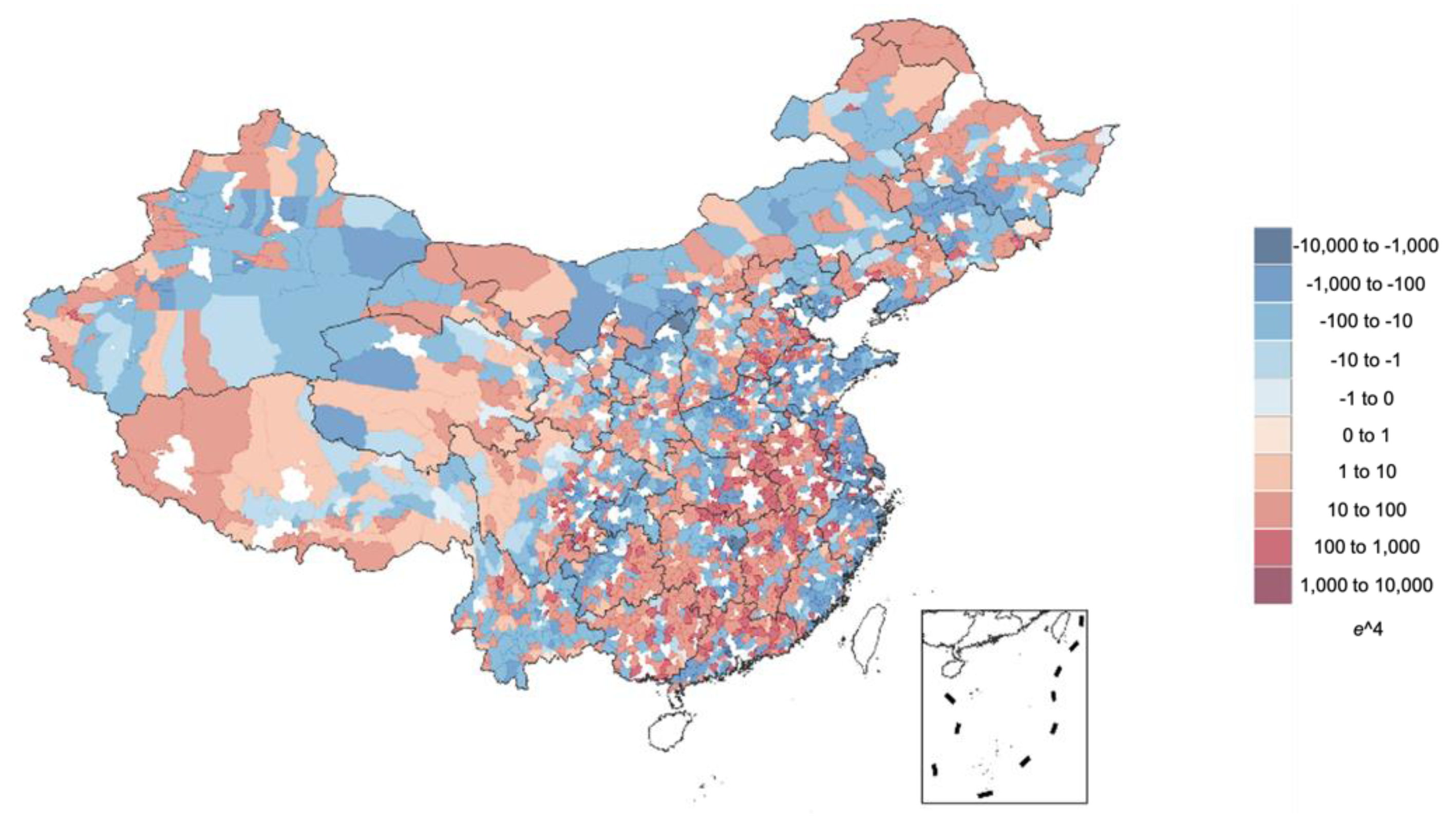
Figure 5 presents the prediction error map of county-level GDP of 2018 in China. The degree of the color reflects the value of the prediction error. Red denotes overestimation, while blue denotes underestimation. According to the prediction error map, we find that estimations of larger counties tend to be more accurate than those of smaller counties. A good reason is that larger counties usually contain more satellite image instances so that the corresponding statistical characteristics are more representative. Another finding is that the proposed framework seems to overpredict in the poorer areas and underpredict in richer areas. In the error map, southeastern coastal areas, the most advanced regions in China, are colored blue, while the middle of China, the less advanced regions, are colored red.
5.2. Ablation Study
To ensure the effectiveness of different modules within our method, we conduct a few ablation experiments. VGG uses only the VGG-16 network, dislodging the attention layer. , , , and n denote methods that remove the sample mean, standard deviation, the Pearson’s correlation, and sample size from statistical characteristics, respectively.
According to the results shown in
Table 3, the insertion of the attention layer effectively improves the R-squared score by 0.02. Meanwhile, any removal of the statistical characteristics decreases the final performance evidently, indicating that each of them makes a meaningful contribution.
5.3. Comparison of Regression Methods
We fed the embedded statistics into different regression models and determined the most suitable method in this case.
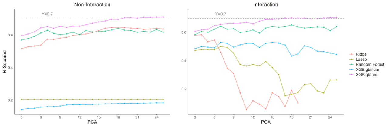
Figure 6 reports the experimental results measured by R-squared. It can be concluded that, in general, random forest and the Xgboost algorithm with a tree kernel (gbtree) perform the best, and that results of gbtree are more stable than those of random forest. The feature interaction process, i.e., construction of extra features, has little influence on these two methods’ performances, probably because random forest and gbtree elect only the most essential features to predict dependent variables. Ridge regression achieves satisfactory results when the original embedded statistics are independent variables, while feature interaction enhances the performance of the Xgboost algorithm with a linear kernel (gblinear). Meanwhile, we find that although feature interaction may enable linear-based models to achieve better results, performances of these models decline rapidly when the dimension of PCA increases.
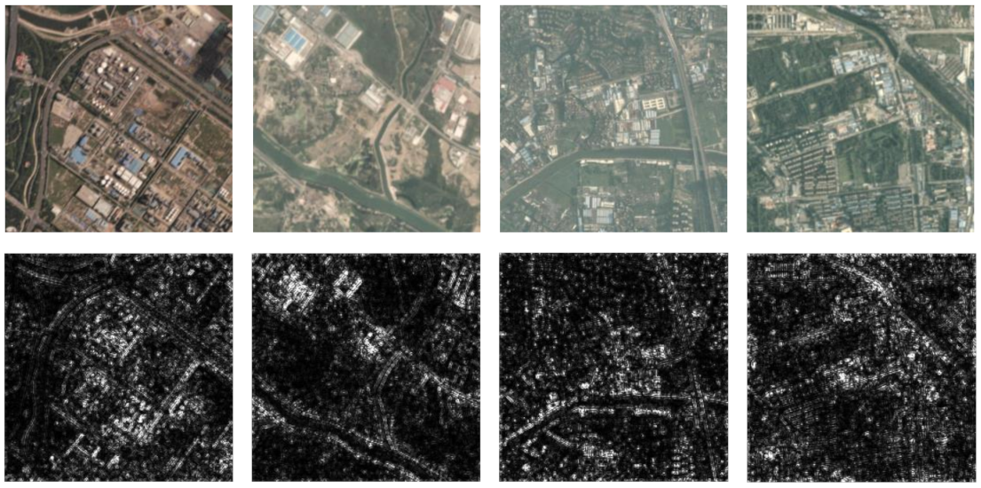
5.4. Gradient Visualization
To explore what our feature extractor focuses on, we conduct gradient visualization with guided back-propagation applied in [
50]. The guided back-propagation method computes the gradient of the target output (nightlight intensity level in our case) concerning the input. Gradients of ReLU functions are overridden so that only non-negative gradients are back-propagated, which is a widely used method in interpreting convolution neural networks. Based on
Figure 7, we can observe the highlighted areas of buildings and the contours of roads in the gradient map, which accords with the perception that a more developed county tends to have denser buildings and advanced transportation systems. It also confirms the validity of using nighttime light intensities as a proxy for economic development levels.
6. Conclusions
This study considered nightlight maps as a proxy of socioeconomic indicators, constructing labels concerning nightlight intensity levels for daytime satellite imagery and training attention-augmented VGG-16 network as a feature extractor. The fixed-length county-level representation was calculated as each county’s statistical characteristics, which were later fed into a simple regressor to predict GDP. Our method yielded a satisfactory performance with an R-squared of 0.71.
Our methods are explainable both quantitatively and qualitatively. The model trained on data from 2017 could achieve relatively high scores in predicting county-level GDP values of 2018. On the other hand, the gradient visualization indicated that the CNN-based classifier performed well in detecting visual patterns that were thought to be closely related to economic development degrees, such as roads and buildings.
Experimental studies confirmed the learning abilities of the VGG structures in our framework. Values of R-squared gradually became stable when the dimension of PCA reduction was greater than 15. The feature interaction process did not contribute much to prediction accuracy, indicating that features learned by the VGG structure were powerfully informative.
This paper contributed to modifying methods that applied remote sensing data in the estimation of socioeconomic indicators. Compared with Jean’s method [
18], our framework is both more applicable to county-level GDP estimation in China and more generalizable. First, Jean’s method was point-to-point, while ours was capable of district-to-point estimation. Concretely speaking, there was a one-to-one relationship between ground-truth data (household wealth) and remote sensing data (paired daytime image and nightlight intensity) in Jean’s method. Consequently, Jean’s method required large volumes of ground-truth socioeconomic data, and the corresponding relationship between socioeconomic data and remote sensing data was strictly constrained. In contrast, thanks to the process of representative statistics calculation, our method could handle the case that a single socioeconomic indicator (or administrative unit) corresponded with variable number of daytime images along with nightlight intensities. Therefore, our method required relatively less ground-truth data and could be applied to estimate socioeconomic indicators at administrative units of variable sizes. Second, since our method enabled all the daytime images and nighttime light intensities belonging to an administrative unit to be used, the estimations were more robust against noise and missing data. Third, the CNN-based classifier in our method was incorporated with the attention mechanism. We successfully augmented the model performance from an R-squared of 0.69 to an R-squared of 0.71 via this module.
Our method still has several limitations. First, missing images degraded model performance, making it unable to learn broad principles around China. Second, while economic development is a continuous process, we applied models trained on data from the previous year to directly predict the next year’s GDP values, leaving the underlying evolution out of consideration. Third, all the images were fed into the same model and, thus, failed to incorporate regional differences.
To the best of our knowledge, there is no previous study that has succeeded in estimating county-level GDP around the Chinese Mainland utilizing daytime and nighttime remote sensing data. This paper filled in this gap, indicating the possibility of convenient socioeconomic data-collecting methods relying on deep learning techniques and remote sensing data. The framework proposed by this paper is still coarse. Nevertheless, it will be fruitful to analyze current experimental results and augment model performance. On the one hand, more accurate estimations are more helpful. On the other hand, research on China, where social development degrees of disparate sub-national regions are measured by the same national economic accounting system, will shed light on the principles of applying remote sensing data in socioeconomic studies.
Author Contributions
Conceptualization, H.L.; methodology, H.L. and X.H.; software, H.L. and X.H.; validation, H.L. and X.H.; formal analysis, H.L. and X.H.; investigation, H.L., X.H., Y.B. and Y.W.; resources, Y.B.; data curation, H.L.; writing—original draft preparation, H.L. and X.H.; writing—review and editing, H.L., X.H., Y.B., X.L.,Y.W. and Y.Z.; visualization, H.L. and X.H.; supervision, Y.B., X.L., H.Y. and Y.Z.; project administration, Y.B.; funding acquisition, Y.B., H.Y., Y.W. and Y.Z. All authors have read and agreed to the published version of the manuscript.
Funding
This research was partly funded by the Fundamental Research Funds for the Central Universities, and the Research Funds of Renmin University of China (17XNLG09), fund for building world-class universities (disciplines) of Renmin University of China.
Data Availability Statement
The data we utilize can be reached at (
www.planet.com, accessed on 11 November 2020). where a python api key is provided to download the images.
Acknowledgments
This work was supported by the Public Computing Cloud, Renmin University of China. We thank Linhao Dong, Ying Hao, Yafeng Wu, Yunhui Xu and Yecheng Tang, students from Renmin University of China; the author gratefully acknowledges the support of the K.C. Wong Education Foundation, Hong Kong.
Conflicts of Interest
The authors declare no conflict of interest.
Abbreviations
The following abbreviations are used in this manuscript:
| CNN | convolutional neural network |
| PCA | principal component analysis |
| GMM | Gaussian mixture model |
| VGG | Visual Geometry Group network |
| VGG-A | Visual Geometry Group network with attention layer |
References
- Bureau, C.N.S. Data Release and Update (10). Available online: http://www.stats.gov.cn/tjzs/cjwtjd/201407/t20140714_580886.html (accessed on 14 October 2020).
- Bureau, C.N.S. National Economic Accounting (17). Available online: http://www.stats.gov.cn/tjzs/cjwtjd/201308/t20130829_74319.html (accessed on 14 October 2020).
- Gao, M.; Fu, H. The overall analysis of current Chinese GDP accounting system. Econ. Theory Econ. Manag. 2014, V34, 5–14. [Google Scholar]
- Liao, X. Considerations on county-level GDP accounting. Mod. Econ. Inf. 2014, 10, 463–465. [Google Scholar]
- Zhang, M. County-level GDP accounting work. Stat. Manag. 2015, 09, 6–7. [Google Scholar]
- Han, S.; Ahn, D.; Cha, H.; Yang, J.; Cha, M. Lightweight and Robust Representation of Economic Scales from Satellite Imagery. Proc. AAAI Conf. Artif. Intell. 2020, 34, 428–436. [Google Scholar] [CrossRef]
- Doll, C.H.; Muller, J.P.; Elvidge, C.D. Night-time Imagery as a Tool for Global Mapping of Socioeconomic Parameters and Greenhouse Gas Emissions. Ambio A J. Hum. Environ. 2000, 29, 157–162. [Google Scholar] [CrossRef]
- Doll, C.N.H.; Muller, J.P.; Morley, J.G. Mapping regional economic activity from night-time light satellite imagery. Ecol. Econ. 2006, 57, 75–92. [Google Scholar] [CrossRef]
- Bagan, H.; Yamagata, Y. Analysis of urban growth and estimating population density using satellite images of nighttime lights and land-use and population data. GIScience Remote Sens. 2015, 52, 765–780. [Google Scholar] [CrossRef]
- Laveesh, B.; Koel, R. Night Lights and Economic Activity in India: A study using DMSP-OLS night time images. Proc. Asia-Pac. Adv. Netw. 2011, 32, 218. [Google Scholar]
- Chaturvedi, M.; Ghosh, T.; Bhandari, L. Assessing Income Distribution at the District Level for India Using Nighttime Satellite Imagery. Proc. Asia Pac. Adv. Netw. 2011, 32, 192–217. [Google Scholar] [CrossRef]
- Wen, W.A.; Hui, C.A.; Li, Z.B. Poverty assessment using DMSP/OLS night-time light satellite imagery at a provincial scale in China. Adv. Space Res. 2012, 49, 1253–1264. [Google Scholar]
- Li, F.; Zhang, X.; Qian, A. DMSP-OLS and NPP-VIIRS night lighting data measurement statistical index capability assessment—Take the Beijing-Tianjin-Hebei area county GDP, population and energy consumption as an example. Mapp. Advis. 2020, 09, 89–93+118. [Google Scholar]
- Elvidge, C.D.; Baugh, K.E.; Zhizhin, M.; Hsu, F.C. Why VIIRS data are superior to DMSP for mapping nighttime lights. Proc. Asia Pac. Adv. Netw. 2013, 35, 62. [Google Scholar] [CrossRef] [Green Version]
- Engstrom, R.; Hersh, J.; Newhouse, D. Poverty from Space: Using High-Resolution Satellite Imagery for Estimating Economic Well-Being; The World Bank: Washington, DC, USA, 2017; Available online: https://elibrary.worldbank.org/doi/abs/10.1596/1813-9450-8284 (accessed on 14 October 2020).
- Rybnikova, N.A.; Portnov, B.A. Estimating geographic concentrations of quaternary industries in Europe using Artificial Light-At-Night (ALAN) data. Int. J. Digit. Earth 2017, 10, 861–878. [Google Scholar] [CrossRef]
- Xie, M.; Jean, N.; Burke, M.; Lobell, D.; Ermon, S. Transfer Learning from Deep Features for Remote Sensing and Poverty Mapping. In Proceedings of the AAAI Conference on Artificial Intelligence, Phoenix, AZ, USA, 12–17 February 2016; Volume 30. [Google Scholar]
- Jean, N.; Burke, M.; Xie, M.; Davis, W.M.; Ermon, S. Combining satellite imagery and machine learning to predict poverty. Science 2016, 353, 790–794. [Google Scholar] [CrossRef] [PubMed] [Green Version]
- Gibson, J.; Olivia, S.; Boe-Gibson, G. Night Lights in Economics: Sources and Uses. LICOS Discuss. Pap. 2020, 34, 955–980. [Google Scholar] [CrossRef]
- Elvidge, C.D.; Imhoff, M.L.; Augh, K.E.B.; Hobson, V.R.; Nelson, I.; Safran, J.; Dietz, J.B.; Tuttle, B.T. Night-time lights of the world: 1994–1995. ISPRS J. Photogramm. Remote Sens. 2001, 56, 81–99. [Google Scholar] [CrossRef]
- Ding, Y.; Yu, Q.; Ling, Y.; Cao, J.; Zhang, H.; Liu, H.; Zhang, E. A study on the pattern of time and space economic development in Shandong Province based on night light data. Mapp. Spat. Geogr. Inf. 2019, 09, 71–73, 77. [Google Scholar]
- Abrahams, A.; Oram, C.; Lozano-Gracia, N. Deblurring DMSP nighttime lights: A new method using Gaussian filters and frequencies of illumination. Remote Sens. Environ. 2018, 210, 242–258. [Google Scholar] [CrossRef]
- Gibson, J.; Olivia, S.; Boe-Gibson, G.; Li, C. Which night lights data should we use in economics, and where? J. Dev. Econ. 2021, 149, 102602. [Google Scholar] [CrossRef]
- Ran, G.; Heilmann, K.; Vaizman, Y. Can Medium-Resolution Satellite Imagery Measure Economic Activity at Small Geographies? Evidence from Landsat In Vietnam; Policy Research Working Paper Series; The World Bank: Washington, DC, USA, 2019. [Google Scholar]
- Chen, X.; William, N. A Test of the New VIIRS Lights Data Set: Population and Economic Output in Africa. Remote Sens. 2015, 7, 4937–4947. [Google Scholar] [CrossRef] [Green Version]
- Chen, X.; Nordhaus, W.D. VIIRS Nighttime Lights in the Estimation of Cross-Sectional and Time-Series GDP. Remote Sens. 2019, 11, 1057. [Google Scholar] [CrossRef] [Green Version]
- Chen, S.; Li, X. Night lighting data predict social and economic activity at different scales. Geography 2020, 40, 1476–1483. [Google Scholar]
- Shi, K.; Yu, B.; Huang, Y.; Hu, Y.; Yin, B.; Chen, Z.; Chen, L.; Wu, J. Evaluating the Ability of NPP-VIIRS Nighttime Light Data to Estimate the Gross Domestic Product and the Electric Power Consumption of China at Multiple Scales: A Comparison with DMSP-OLS Data. Remote Sens. 2014, 6, 1705–1724. [Google Scholar] [CrossRef] [Green Version]
- Sun, Y.; Liu, X.; Su, Y.; Shuang, X.V.; Ji, B.; Zhang, Z. Based on night light data, the level of county-level urbanization in Anhui Province is estimated. J. Earth Inf. Sci. 2020, 22, 89–99. [Google Scholar]
- Li, Y.; Gang Cheng, J.Y.; Yuan, D. The fine simulation of regional economic spatial pattern supported by night light remote sensing data is an example of Henan Province. Reg. Res. Dev. 2020, 04, 41–47. [Google Scholar]
- Vogel, K.B.; Goldblatt, R.; Hanson, G.H.; Khandelwal, A.K. Detecting Urban Markets with Satellite Imagery: An Application to India; NBER Working Papers; National Bureau of Economic Research: Cambridge, MA, USA, 2018. [Google Scholar]
- Abitbol, J.L.; Karsai, M. Socioeconomic Correlations of Urban Patterns Inferred from Aerial Images: Interpreting Activation Maps of Convolutional Neural Networks. arXiv 2020, arXiv:2004.04907. [Google Scholar]
- Robinson, C.; Hohman, F.; Dilkina, B. A Deep Learning Approach for Population Estimation from Satellite Imagery. In Proceedings of the 1st ACM SIGSPATIAL Workshop, Redondo Beach, CA, USA, 7 November 2017; pp. 47–54. [Google Scholar]
- Doupe, P.; Bruzelius, E.; Faghmous, J.; Ruchman, S.G. Equitable Development through Deep Learning: The Case of Sub-National Population Density Estimation. In Proceedings of the 7th Annual Symposium on Computing for Development (ACM DEV ’16), Nairobi, Kenya, 18–20 November 2016; Association for Computing Machinery: New York, NY, USA, 2016. [Google Scholar] [CrossRef]
- Hu, W.; Patel, J.H.; Robert, Z.A.; Novosad, P.; Asher, S.; Tang, Z.; Burke, M.; Lobell, D.; Ermon, S. Mapping Missing Population in Rural India: A Deep Learning Approach with Satellite Imagery. In Proceedings of the 2019 AAAI/ACM Conference on AI, Ethics, and Society, Honolulu, HI, USA, 27–28 January 2019; pp. 353–359. [Google Scholar]
- Babenko, B.; Hersh, J.; Newhouse, D.; Ramakrishnan, A.; Swartz, T. Poverty Mapping Using Convolutional Neural Networks Trained on High and Medium Resolution Satellite Images, With an Application in Mexico. arXiv 2017, arXiv:1711.06323. [Google Scholar]
- Han, S.; Ahn, D.; Park, S.; Yang, J.; Lee, S.; Kim, J.; Yang, H.; Park, S.; Cha, M. Learning to score economic development from satellite imagery. In Proceedings of the 26th ACM SIGKDD International Conference on Knowledge Discovery & Data Mining, Virtual Event, CA, USA, 23–27 August 2020; pp. 2970–2979. [Google Scholar]
- ImageNet Large Scale Visual Recognition Challenge. Int. J. Comput. Vis. 2015, 115, 211–252. [CrossRef] [Green Version]
- Krizhevsky, A.; Sutskever, I.; Hinton, G.E. Imagenet classification with deep convolutional neural networks. Adv. Neural Inf. Process. Syst. 2012, 25, 1097–1105. [Google Scholar] [CrossRef]
- Ni, Y.; Li, X.; Ye, Y.; Li, Y.; Chu, D. An Investigation on Deep Learning Approaches to Combining Nighttime and Daytime Satellite Imagery for Poverty Prediction. IEEE Geosci. Remote Sens. Lett. 2020, 1–5. [Google Scholar] [CrossRef]
- Huang, G.; Liu, Z.; Laurens, V.; Weinberger, K.Q. Densely Connected Convolutional Networks; IEEE Computer Society: Los Alamitos, CA, USA, 2016. [Google Scholar]
- He, K.; Zhang, X.; Ren, S.; Jian, S. Identity Mappings in Deep Residual Networks; Springer: Cham, Switzerland, 2016. [Google Scholar]
- Head, A.; Manguin, M.; Tran, N.; Blumenstock, J.E. Can Human Development Be Measured with Satellite Imagery? In Proceedings of the Ninth International Conference on Information and Communication Technologies and Development (ICTD ’17), Lahore, Pakistan, 16–19 November 2017; Association for Computing Machinery: New York, NY, USA, 2017. [Google Scholar] [CrossRef]
- Yeh, C.; Perez, A.; Driscoll, A.; Azzari, G.; Burke, M. Using publicly available satellite imagery and deep learning to understand economic well-being in Africa. Nat. Commun. 2020, 11, 2583. [Google Scholar] [CrossRef] [PubMed]
- Biernacki, C.; Celeux, G.; Govaert, G. Assessing a mixture model for clustering with the integrated completed likelihood. IEEE Trans. Pattern Anal. Mach. Intell. 2000, 22, 719–725. [Google Scholar] [CrossRef]
- Pypi. GeoPandas. Available online: https://pypi.org/project/geopandas/ (accessed on 11 November 2020).
- Simonyan, K.; Zisserman, A. Very deep convolutional networks for large-scale image recognition. arXiv 2014, arXiv:1409.1556. [Google Scholar]
- Abdi, H.; Williams, L.J. Principal component analysis. Wiley Interdiscip. Rev. Comput. Stat. 2010, 2, 433–459. [Google Scholar] [CrossRef]
- Kingma, D.P.; Welling, M. Auto-encoding variational bayes. arXiv 2013, arXiv:1312.6114. [Google Scholar]
- Arriaga, O.; Valdenegro-Toro, M.; Plöger, P. Real-time convolutional neural networks for emotion and gender classification. arXiv 2017, arXiv:1710.07557. [Google Scholar]
| Publisher’s Note: MDPI stays neutral with regard to jurisdictional claims in published maps and institutional affiliations. |
© 2021 by the authors. Licensee MDPI, Basel, Switzerland. This article is an open access article distributed under the terms and conditions of the Creative Commons Attribution (CC BY) license (https://creativecommons.org/licenses/by/4.0/).


 ,
, 


