Detecting Winter Cover Crops and Crop Residues in the Midwest US Using Machine Learning Classification of Thermal and Optical Imagery

Abstract

Cover crops are an increasingly popular practice to improve agroecosystem resilience to climate change, pests, and other stressors. Despite their importance for climate mitigation and soil health, there remains an urgent need for methods that link winter cover crops with regional-scale climate mitigation and adaptation potential. Remote sensing is ideally suited to provide these linkages, yet, cover cropping has not been analyzed extensively in remote sensing research. Methods used for remote sensing of crops from satellites traditionally leverage the difference between visible and near-infrared reflectance to isolate the signal of photosynthetically active vegetation. However, using traditional greenness indices like the Normalized Difference Vegetation Index (NDVI) for remotely sensing winter vegetation, such as winter cover crops, is challenging because vegetation reflectance signals are often confounded with reflectance of bare soil and crop residues. Here, we present new and established methods of detecting winter cover crops using remote sensing observations. We find that remote sensing methods that incorporate thermal data in addition to traditional reflectance metrics are best able to distinguish between winter farm management practices. We conclude by addressing the potential of existing and upcoming hyperspectral and thermal missions to further assess agroecosystem function in the context of global change.

1. Introduction

As one of the most intensively managed landscapes worldwide, agroecosystems provide a crucial opportunity to mitigate greenhouse gas emissions at a global scale [1]. One of the most promising climate mitigation and adaptation interventions in agroecosystems is the practice of cover cropping [2], where farmers plant a non-commercial crop during fallow periods when the soil is typically bare between cash crop harvest and the following season’s planting. Cover cropping, alongside zero tillage and mulching, represent a set of practices that are jointly referred to as conservation agriculture, which is practiced by farmers worldwide [3]. In temperate climates, such as the U.S. Midwest (also known as ‘the Corn Belt’), cover cropping occurs during winter when growing conditions for vegetation is minimized. Winter cover crops are crucial to climate mitigation because of their potential to dramatically increase soil carbon sequestration [2]. In addition, they offer important climate adaptation benefits to help farmers adapt to prolonged drought and more intense precipitation events [4,5]. Even though cover crops’ mitigation and adaptation benefits are touted as a win-win opportunity (e.g., [6,7,8]), research to detect and analyze the effects of winter cover crops at large spatial and temporal scales remains in the early stages.

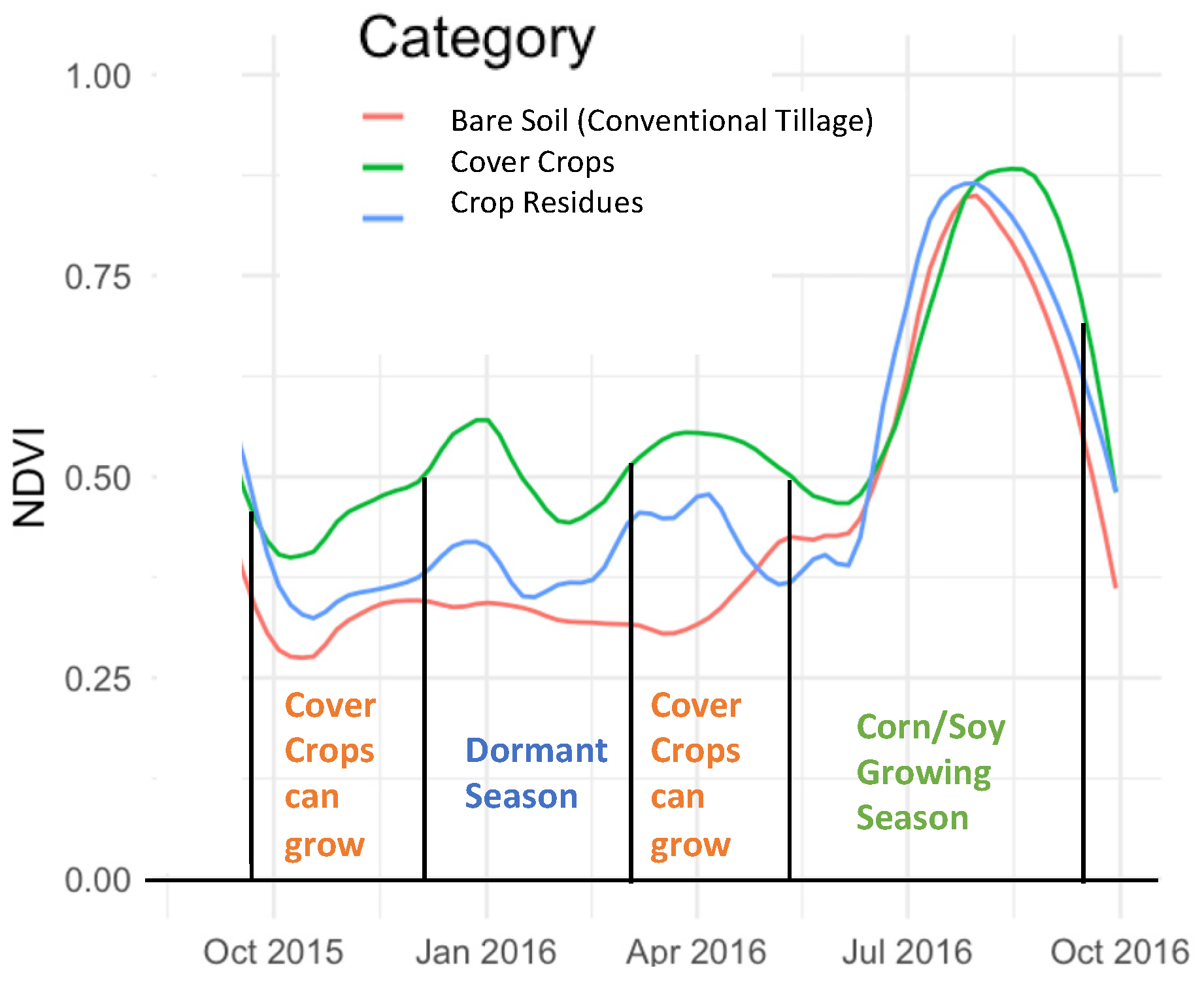
Large-scale analysis of cover crops requires improving upon current multispectral remote sensing techniques to extend our existing understanding of cover crops gained from field-scale research. Cover crops have not been analyzed extensively in remote sensing research, but the field has been growing rapidly in the past decade due to both increased availability of hyperspectral and high-resolution imagery and increased adoption of the practice by farmers [9]. In the U.S. Midwest, cover crops stand out because so much biomass disappears from monocultural agroecosystems after fall harvest that they are the only remaining active vegetation on farmlands (excluding pasturelands; Figure 1). Because of this dynamic, many studies have focused primarily on modifying traditional greenness indices, such as NDVI, to compare different combinations of visible and infrared bands to distinguish between active and inactive vegetation [10,11,12,13,14,15,16,17] (Table 1).

Prabhakara et al. (2015) compared relationships between 10 different visible range and near infrared (NIR) indices and percent ground cover and biomass of winter cover crops [10]. They found that NDVI and the triangular vegetation index (TVI), which is the hypothetical triangle created by green peak reflectance, red minimum chlorophyll absorption bands, and the NIR edge, provided the most accurate estimates of cover crop biomass and percent cover (Table 1). One of the difficulties in relying solely on traditional greenness indices for detecting cover crops is that they are intermixed in agricultural fields alongside bare soils and crop residues, which are the dormant and decaying remains of harvested crops left in the field. Traditional greenness indices have difficulty distinguishing between bare soils and crop residues (Figure 1, [11]). Furthermore, cover crops also become dormant with cold winter temperatures or can be seeding after dormancy, emerging only in the spring [18]. Recently, time series methods to identify cover crops based on phenology from multiple sensors have successfully predicted cover crop and cover crop residue cover over large spatial scales [19] and cover crop end of season [15].

Using wavelengths beyond those in the visible and NIR portions of the electromagnetic spectrum is a promising strategy to differentiate between non-photosynthetically active vegetation (i.e., crop residues) and bare soils in agroecosystems. By incorporating information from wavelengths in the shortwave infrared (SWIR), cellulose and lignin absorption features of crop residues can be detected and used to differentiate them from bare soils ([11,20,21,22]; Table 1). Hively et al. (2018) compared the performance of the normalized difference tillage index (NDTI) index from Landsat observations and six WorldView-3 SWIR indices to map the spatial pattern of crop residues [23]. Their results suggested that two SWIR indices of Lignin Cellulose Absorption Index (LCA) and Shortwave Infrared Normalized Difference Residue Index (SINDRI) performed most accurately (Table 1). Similarly, Sonmez and Slater (2016) found that SWIR-based Cellulose Absorption Index detected crop residue and tillage practices better than three vegetation indices [21]. Rather than estimating percent of ground cover or biomass of cover crops, machine learning methods can predict the presence of cover crops anywhere on the landscape using only remotely sensed data. Seifert et al. 2018 used a random forest classification to incorporate the NDVI and SWIR bands along with additional parameters, such as elapsed days, to classify winter cover crops [24]. We note that the term “Growing Degree Days” generally incorporate a temperature threshold calculation, and henceforth refer to GDD as defined by Seifert et al. (2018) as “Elapsed Days”.

Table 1. Summary of recent (2015 and after) efforts to estimate winter cover crops and crop residues in agricultural farm fields.

Target Parameter	Location	Satellite Data	Most Predictive Indices for Target Parameter	Reference
Crop Residue	Canada	EO-1 Hyperion	SWIR (shortwave infrared) spectral bands	Bannari et al., 2015 [20]
Crop Residue, Cover Crop	Pennsylvania, USA	Landsat + SPOT	NDTI (Normalized Difference Tillage Index) mean NDVI, GDD (“Growing Degree Days”)	Hively et al., 2015 [11]
Crop Residue, Tillage Practices	Ohio, USA	Landast + EO-1 Hyperion	CAI (cellulose absorption index)	Sonmez and Slater 2016 [21]
Crop Residue	Maryland, USA	Landsat + WorldView-3 SWIR	SINDRI (Shortwave Infrared Normalized Difference Residue Index), LCA (Lignin Cellulose Absorption)	Hively et al., 2018 [23]
Crop Residue	Maryland, USA	Worldview-3	Moisture corrected SINDRI	Quemada et al., 2018 [25]
Cover Crop	Marland, USA	16-band CROPSCAN Imagery	NDVI, TVI (Triangular vegetation index), GDD	Prabhakara et al., 2015 [10]
Cover Crop	Kansas, USA & Ukrain	MODIS	GDD, maximum NDVI	Skakun et al., 2017 [14]
Cover crop	Midwestern USA	Landsat + MODIS	Elapsed Days, maximum NDVI	Seifert et al., 2018 [24]
Cover Crop	Maryland, USA	Landsat	GDD	Hively et al., 2020 [26]
Cover Crop	Maryland, USA	Landsat + Sentinel-2	Maximum seasonal NDVI	Thieme et al., 2020 [12]
Cover Crop	Corn Belt regions, USA	Landsat, Sentinel, MODIS	NDVI (timing and intensity)	Hagen et al., 2020 [19]
Cover Crop	Eastern Netherlands	Sentinel-2	GDD, NDVI (timing and intensity)	Fan et al., 2020 [27]
Cover Crop (senescence)	Washington, DC, USA	VENµS and Sentinel-2	NDVI (downward trend)	Gao et al., 2020 [15]

Table 1. Summary of recent (2015 and after) efforts to estimate winter cover crops and crop residues in agricultural farm fields.

Target Parameter	Location	Satellite Data	Most Predictive Indices for Target Parameter	Reference
Crop Residue	Canada	EO-1 Hyperion	SWIR (shortwave infrared) spectral bands	Bannari et al., 2015 [20]
Crop Residue, Cover Crop	Pennsylvania, USA	Landsat + SPOT	NDTI (Normalized Difference Tillage Index) mean NDVI, GDD (“Growing Degree Days”)	Hively et al., 2015 [11]
Crop Residue, Tillage Practices	Ohio, USA	Landast + EO-1 Hyperion	CAI (cellulose absorption index)	Sonmez and Slater 2016 [21]
Crop Residue	Maryland, USA	Landsat + WorldView-3 SWIR	SINDRI (Shortwave Infrared Normalized Difference Residue Index), LCA (Lignin Cellulose Absorption)	Hively et al., 2018 [23]
Crop Residue	Maryland, USA	Worldview-3	Moisture corrected SINDRI	Quemada et al., 2018 [25]
Cover Crop	Marland, USA	16-band CROPSCAN Imagery	NDVI, TVI (Triangular vegetation index), GDD	Prabhakara et al., 2015 [10]
Cover Crop	Kansas, USA & Ukrain	MODIS	GDD, maximum NDVI	Skakun et al., 2017 [14]
Cover crop	Midwestern USA	Landsat + MODIS	Elapsed Days, maximum NDVI	Seifert et al., 2018 [24]
Cover Crop	Maryland, USA	Landsat	GDD	Hively et al., 2020 [26]
Cover Crop	Maryland, USA	Landsat + Sentinel-2	Maximum seasonal NDVI	Thieme et al., 2020 [12]
Cover Crop	Corn Belt regions, USA	Landsat, Sentinel, MODIS	NDVI (timing and intensity)	Hagen et al., 2020 [19]
Cover Crop	Eastern Netherlands	Sentinel-2	GDD, NDVI (timing and intensity)	Fan et al., 2020 [27]
Cover Crop (senescence)	Washington, DC, USA	VENµS and Sentinel-2	NDVI (downward trend)	Gao et al., 2020 [15]

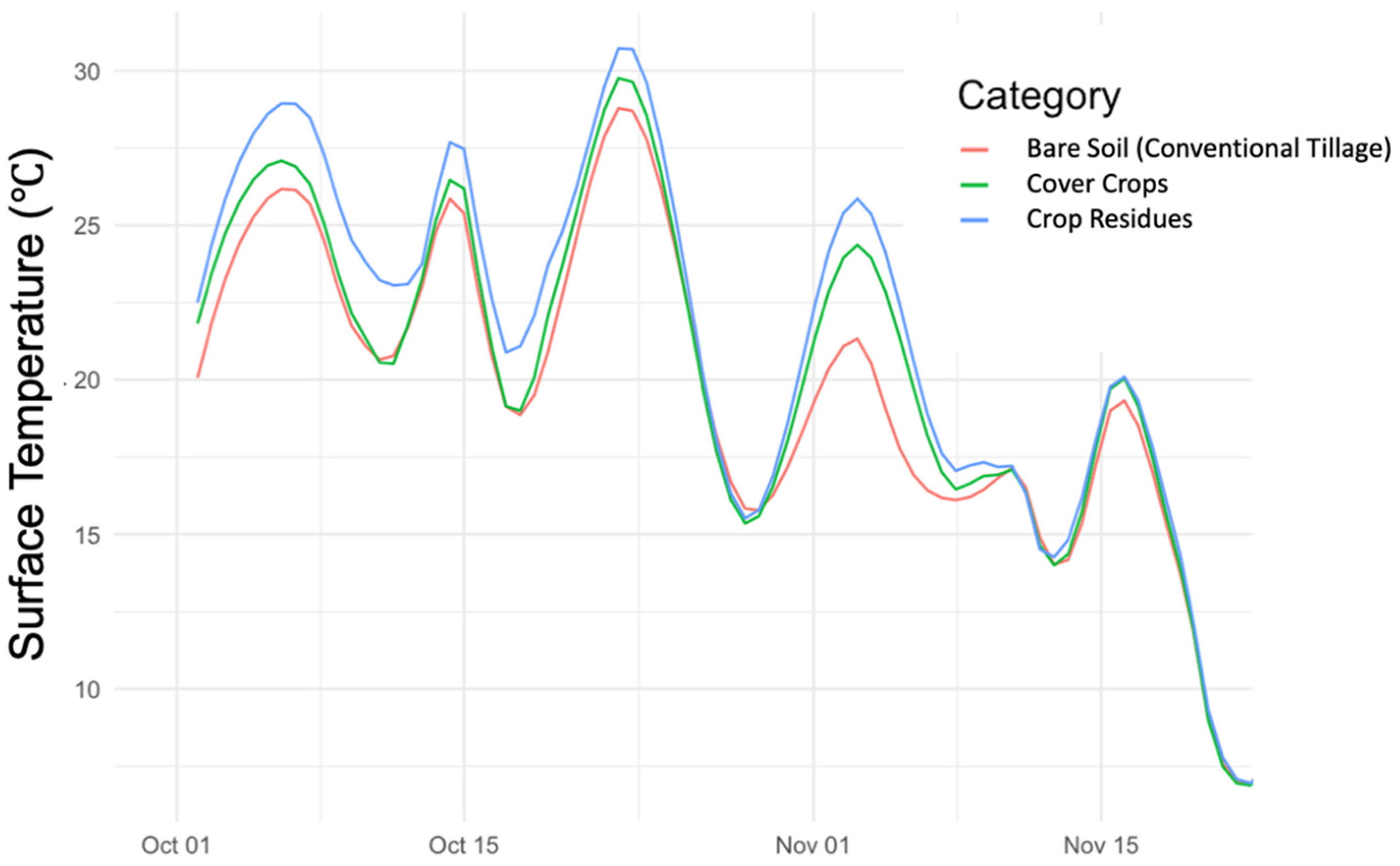
These promising efforts indicate that remote sensing can be an effective approach to analyze cover cropping and related conservation agriculture practices at regional scales. However, most studies have still largely limited their approaches to smaller geographic areas, and few have taken advantage of the potential of machine learning models to explicitly predict cover crop presence in agroecosystems. Additionally, applications of thermal remote sensing in agriculture have been limited compared to those using optical remote sensing data [28]. Thermal remote sensing provides information about temperatures on the earth’s surface, which is linked to landscape-level patterns and processes like vegetation cover [29], plant activity [30], and vegetation water stress [31,32]. While traditionally challenging to process at fine scales, recent developments including the Landsat Provisional Surface Temperature (ST) product [33], provide a key opportunity to test the potential benefits of thermal data for prediction of agroecosystem practices. A preliminary exploration of the differences in ST between winter cover crops, crop residues, and bare soils indicates consistent temperature differences in the fall that could be leveraged by machine learning classification algorithms (Figure 2).

Our ability to monitor cover crop adoption and predict the benefits of widespread cover crop use as a potential climate mitigation strategy depends on our ability to accurately detect cover crops across regional scales. In this paper we evaluate the predictive capacity of established and novel remote-sensing-based metrics for detecting cover crops using a series of machine learning models. The goal of this work is to assess which regions of the electromagnetic spectrum and indices are most effective for detecting cover crops and crop residues. We developed two suites of machine learning models: a two-class model to predict the presence or absence of winter cover crops, and a three-class model to classify winter cover crops, crop residues, and bare soils. The model inputs increase in complexity from traditional greenness indices, to adding SWIR and then thermal data with the Landsat ST product. We anticipate that the addition of thermal data will improve detection of cover crops because cover crops are generally warmer than bare soil in the autumn (Figure 2). We also anticipate that adding SWIR will improve model ability to distinguish between cover crops and crop residues. Our overarching goal is to develop a comprehensive methodology to quantify observed and potential benefits of winter cover crop adoption at spatial and temporal scales relevant for land management.

2. Materials and Methods

We obtained Landsat Operational Land Imager (OLI) and TIRS (Thermal Infrared Sensor) observations and the Landsat Provisional ST product for the 2015–2016 growing season and calculated vegetation-relevant metrics in the visible, near-infrared, shortwave infrared, and thermal regions. Using these remotely sensed input data and ground-truth information from windshield surveys (Section 2.1), we created a series of random forest models to classify (1) the presence/absence of cover crops; and (2) distinguish between cover crops, crop residues, and bare soil/conventional tillage. We then built models with increasing complexity to assess the additional value of each wavelength region beyond simple greenness (NDVI). Remote sensing classification models were assessed using both model accuracy and Cohen’s Kappa.

2.1. Survey Data

Indiana is in the Midwestern United States, a temperate region that produces about one-quarter of the world’s annual soybean supply and one-third of the world’s annual maize supply [34]. There are over 127 million acres of agricultural land in the Midwest, 75% of which is used for corn and soybeans, and the remaining 25% is used to produce a variety of crops including alfalfa, tobacco, and wheat [35]. The most popular cover crops in Indiana are fall-seeded cereals like rye and wheat [36]. Cash crops are typically planted in mid-April to early May, and harvested in mid-September to mid-October.

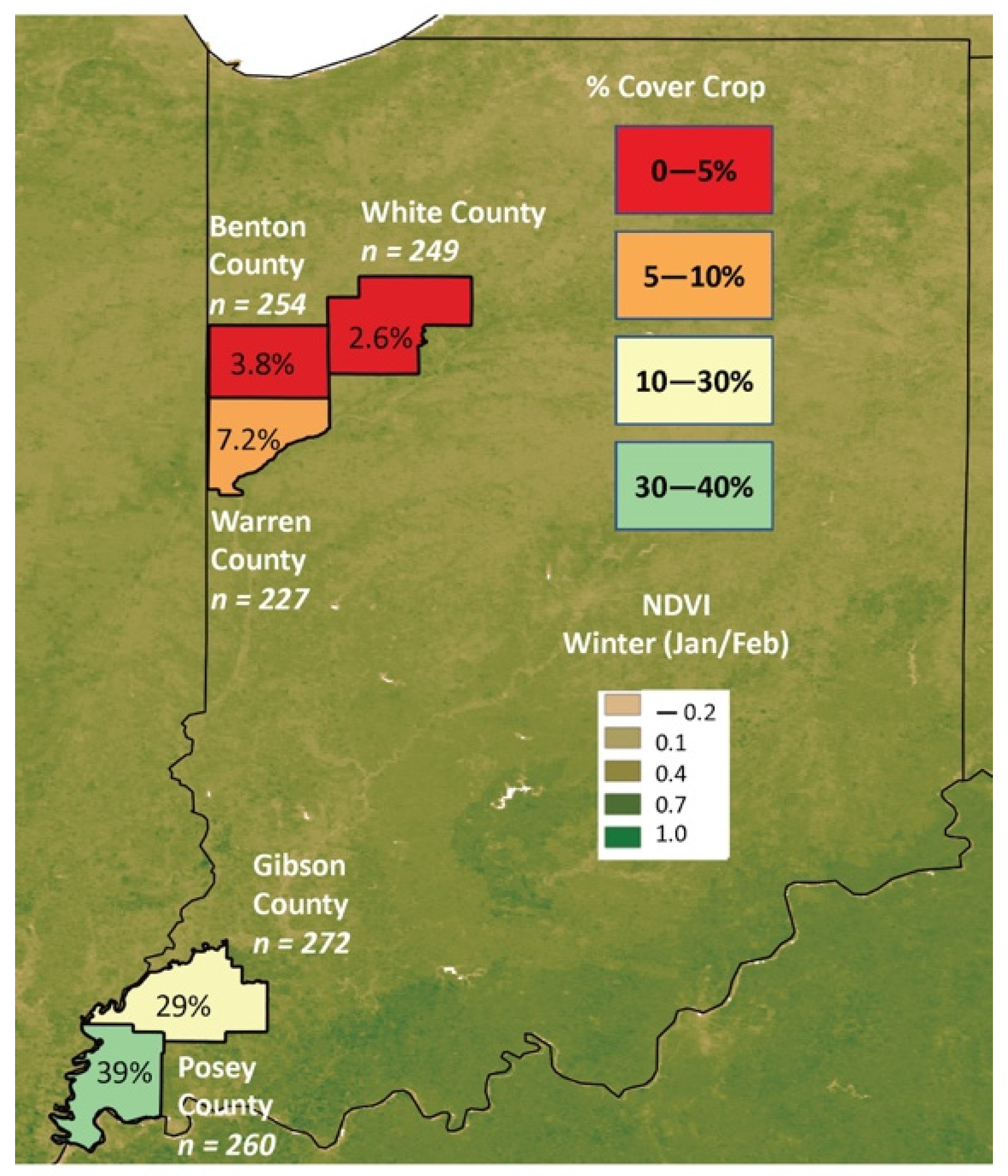
Our study draws on field validation data from fall windshield surveys collected by the U.S. Department of Agriculture’s Natural Resources Conservation Service (NRCS) across five counties in Indiana, USA. A team of surveyors drives along prescribed transects and manually records cover crop presence and species, crop residue presence, and prior cash crop, among other metrics [37]. We obtained the survey transect data from five selected counties in Indiana (Figure 3), resulting in data from a total of 1262 ground-truthing fields. We aggregated the species-specific cover crop observations into presence/absence data. The counties differed in their rates of cover cropping, but the number of transect points documenting the presence of cover crops within each county were generally representative of that county’s cover cropping rate. (

Table 2. Representativeness of study counties in Indiana. The number of GPS points designated as ‘cover crop’ in transects in each county are compared to overall estimates of cover cropping rates in study counties after both corn and soy growing seasons. Total n = 1262.

County	Cover Cropped (Approximate % of GPS Points in Ground Surveys)	Reported County Cover Cropping Rate (from Indiana Conservation Tillage Program Estimates)
Benton	3.8%	5% (corn), 6% (soy)
Gibson	29%	27% (corn), 14% (soy)
Posey	39%	34% (corn), 22% (soy)
Warren	7.2%	7% (corn), 7% (soy)
White	2.6%	3 % (corn), 4% (soy)

). Survey transect data were processed in ESRI ArcGIS version 10.1. Specifically, 120 m buffers (polygons) were created around all 1262 GPS transect points, avoiding roads, ditches, and other non-agricultural land cover areas. We chose 120 m to keep the polygons as close to the roadside points as possible and to maintain proximity to the transect points, while permitting enough pixels to represent the ground. The average spectral signature for each band within a 40 m buffer around the 120 m buffer centroid was used to calculate band metrics in Table 2. These data were then used to train our random forest classification models.

2.2. Remote Sensing Analyses

2.2.1. Landsat OLI Observations

We obtained HLS2 (Harmonized Landsat Sentinel 2 Data) BRDF-adjusted (Bidirectional Reflectance Distribution Function) L30 (Landsat-8 OLI harmonized surface reflectance resampled at 30 m over the Sentinel-2 tiling system) for all of Indiana [38] for the study year (2015–2016 growing season). We used the HLS product to facilitate future incorporation of the HLS S30 (Sentinel-2 30 m) product, which was not used in the present study. The study area required the download of 12 tiles: 16SDH, 16SEH, 16SFH, 16SDJ, 16SEJ, 16SFJ, 16TFK, 16TEK, 16TDK, 16TDL, 16TEL, and 16TFL. Data were reprojected using the ‘gdalwarp’ command in the ‘rgdal’ package, version 1.5–18 [39] in R [40]. For all scenes, we created a cloud mask based on the corresponding Quality Assessment (QA) layer that filtered out pixels with Cirrus (bit 0), Cloud (bit 1), or Adjacent Cloud (bit 2) according to the recommendations in the HLS Product user’s guide Version 1.4 [41]. Data were compiled to represent the hydrologic year rather than the calendar year; the 2016 water year runs from 1 October 2015 through 30 September 2016.

2.2.2. Landsat Analysis-Ready Data

The Landsat ST product and associated Quality Assessment (QA) layers were obtained from the U.S. Landsat Analysis Ready Data product bundle. Only surface temperature estimates from the Landsat 8 thermal imager were used in this analysis for continuity with the OLI observations. The ST data are produced at 100 m resolution every 16 days. Broadly, the surface temperature algorithm uses Level-1 thermal infrared bands from the Thermal InfraRed Sensor (TIRS), along with other ancillary inputs, to estimate surface temperature in Kelvin for the terrestrial land surface. More algorithm details can be found in [33]. For all scenes, we filtered out pixels with high uncertainty in the ST based on the ST QA layer (>70%). Data were compiled to represent the hydrologic year and converted to degrees Celsius.

2.2.3. Band Math for Random Forest Inputs

We applied calculations to the L30 Bands and ST to obtain the metrics described in

Table 3. Band math calculations for Landsat post-harvest relevant metrics. Landsat observations for a total of n = 1262 points were used.

Metric	Math Applied	Reference(s)	Models Included
NDVI	Maximum of fall observations (1 October—1 December)	Skakun et al., 2017 [14]	First level
NDVI	• Minimum of fall observations • Median of fall observations • Amplitude (annual max (1 October—30 September)—fall max (1 October—1 December)) • Annual maximum of NDVI (1 October—30 September) • Ratio of Fall maximum NDVI to annual maximum NDVI (1 October—30 September)	Hagen et al., 2020 [19]	Second level
B3 (Green Band)	Median of fall Observations (1 October—1 December)	Seifert et al., 2018 [24]	Second level
B5 (NIR Band)	Median of fall Observations (1 October—1 December)	Seifert et al., 2018 [24]	Second level
B6 (SWIR 1 Band)	Median of fall Observations (1 October—1 December)	Seifert et al., 2018 [24]	Second level
Elapsed Days	Sum from 11/1 to annual maximum NDVI image date (1 October—30 September)	Seifert et al., 2018 [24]	Second level
Normalized Difference Tillage Index (NDTI)	Median of fall Observations (1 October—1 December)	Hively 2019 [42]	Third level
Simple Tillage Index (STI)	Median of fall Observations (1 October—1 December)	Van Deventer 1997 [43]	Third level
Surface Temperature (ST)	Median of fall Observations (1 October—1 December)	Cook et al., 2014 [33] (Product)	Fourth level
B10 (Thermal infrared 2 Band)	• Median of fall Observations (1 October—1 December) • Annual maximum of B10 (1 October—30 September) • Thermal Ratio (ratio of fall maximum B10 to annual maximum B10).	Developed for this paper	Fourth level

. We transformed Landsat bands to calculate both well-established and novel band metrics that we used as input data for the random forest classification models. We obtained NDVI using the standard Landsat 8 formulation

$$\mathrm{NDVI}=\frac{\mathrm{Band} 5-\mathrm{Band} 4}{\mathrm{Band} 5+\mathrm{Band} 4 }$$

(1)

where Bands 5 and 4 represent the NIR and Red bands, respectively. Further calculations performed on NDVI timeseries are described in Table 2. To calculate the Simple Tillage Index (STI) and Normalized Difference Tillage Index (NDTI), we used the following equations

$$\mathrm{STI}=\frac{\mathrm{Band} 6}{\mathrm{Band} 7}$$

(2)

$$\mathrm{NDTI}=\frac{\mathrm{Band} 6-\mathrm{Band} 7}{\mathrm{Band} 6+\mathrm{Band} 7}$$

(3)

where bands 6 and 7 are SWIR 1 and SWIR 2, respectively. To calculate elapsed days, we counted the number of days between 11/1 of 2015 and the date of maximum NDVI for each pixel

$$\mathrm{Elapsed} \mathrm{Days}={\displaystyle {\sum }_{11/1}^{Date Max NDVI}}ndays$$

(4)

in the formulation of Seifert et al. (2018) [24].

2.3. Random Forest Classification

2.3.1. Model Building

We used a machine learning classification approach in this study to assess cover crop presence on the landscape and distinguish cover crops from crop residues and bare soils. Machine learning is a powerful technique that allows an algorithm to ‘learn’ relationships between output classes (e.g., cover crops vs. bare soil) and input features (e.g., remotely sensed metrics) to classify novel input data. We used random forest, which is a supervised learning algorithm. For classification problems, random forest constructs an ensemble of decision trees based on input features during training, then aggregates votes from individual trees to determine the final predicted class. One strength of random forest (as opposed to other machine learning algorithms) is that the models are interpretable, in that the trained model can be used to gain insight into the relationship between features and classes using variable importance metrics [44].

Here, we developed both two- and three-class random forest models to predict winter land cover and land use practices in the U.S. state of Indiana. The two-class model was trained to predict the presence or absence of winter cover crops across the landscape. The three-class model aimed to distinguish between bare soil (conventional tillage), crop residues, and winter cover crops. To assess the value of adding observations and indices from additional regions of the electromagnetic spectrum, four iterations of each model were run with an increasingly complex set of input parameters. The four levels of complexity were as follows:

• First level: NDVI—we used the maximum of fall (1 October–1 December) NDVI observations for each pixel.
• Second level: VisNIR—we used bands and indices from the visible and near infrared regions of the spectrum (see Table 2), in addition to the NDVI from the first level.
• Third level: SWIR—we added two tillage indices, based on the shortwave infrared bands (see Equations (2) and (3) to the input datasets in the third level of complexity, in addition to all metrics in levels 1 and 2.
• Fourth level: ST (Thermal)—we added the median of fall observations (October—1 December) and the absolute maximum ST from the Landsat provisional surface temperature product to the input datasets in this fourth and final level of complexity, in addition to all metrics in levels 1, 2, and 3.

Random forest models were created using the ‘caret’ package in R [45]. Because the classes were highly imbalanced (i.e., there were many more non-cover crop points than points with winter cover crops), we up-sampled the cover crop points in the training dataset to achieve balanced classes for model training. Specifically, the minority class (cover crops) was sampled with replacement to make the class distributions equal. In random forest model development, we conducted repeated cross-validation of 80% of the training data with 10 folds and 10 repeats. The number of trees (ntree) was set at 500 for all models. We also created a grid of hyper-parameter values that allowed the ‘mtry’ metric, which is the number of variables available for splitting at each tree node, to vary from 1 to 16 (the total number of variables in our input dataset). The models presented in

Table 4. Training accuracy of cover crop detection algorithms when based on increasingly extensive range of wavelengths in the input datasets (total n = 989). We report the overall model accuracy, the value of the kappa statistic for the cover crop class, and the optimal mtry value used for the final model.

Model	First Level: NDVI	Second Level: VisNIR	Third Level: SWI	Fourth Level: Thermal ST
Two-class model: Cover crop presence/absence	Acc = 89.7% k = 0.79 mtry = 1	Acc = 95.2% k = 0.91 mtry = 2	Acc = 95.4% k = 0.91 mtry = 2	Acc = 95.5% k = 0.91 mtry = 2
Three-class model: Cover crop vs. residue vs. bare soil (conventional till)	Acc = 72.1% k = 0.58 mtry = 2	Acc = 77.1% k = 0.66 mtry = 1	Acc = 78.9% k = 0.68 mtry = 1	Acc = 79.7% k = 0.70 mtry = 3

are models with the highest accuracy and kappa.

2.3.2. Model Validation

In addition to reporting model statistics on the 20% of the validation data left out during model building, we also applied the models to all of Posey County Indiana and evaluated model performance against the transect data. The latter is a more difficult classification task for the machine learning algorithm because it must implement the algorithm to classify every pixel across the county. The ‘best’ models were selected based on both accuracy and Cohen’s Kappa statistic:

$$\kappa =\frac{P_o-P_e}{1-P_e}$$

(5)

where P_o is the relative observed agreement, and P_e is the expected agreement. There is no standard scale for interpreting kappa values. The higher the kappa value, the better the match between machine learning classification results and the ground truth data. Here, we consider Landis and Koch’s interpretation for kappa values, where: 0–0.20 is slight, 0.21–0.40 is fair, 0.41–0.60 is moderate, 0.61–0.80 is substantial, and 0.81–1 is ‘almost perfect’ [46].

Overall accuracy was evaluated as

$$\mathrm{Overall} \mathrm{Accuracy}=\frac{\mathrm{TP}+\mathrm{TN}}{\mathrm{TP}+\mathrm{TN}+\mathrm{FP}+\mathrm{FN}}$$

(6)

where true positive (TP); true negative (TN); false positive (FP); and false negative (FN) are all possibilities for the relationship between the predicted condition (modeled class) and true condition (ground truth class). A ‘false positive’ is also known as a ‘Type I statistical error’ and ‘false negative’ is known as a ‘Type II statistical error’. Because it is more important for our cover crop detection model to detect the presence of cover crops, rather than detect the presence of bare soil/conventional tillage, we also report the Positive Class Accuracy

$$\mathrm{Positive} \mathrm{Class} \mathrm{Accuracy}=\frac{\mathrm{TP}}{\left(\mathrm{TP}+\mathrm{FN}\right)}$$

(7)

3. Results

3.1. Within-Model Training Accuracy Model Results

Overall, models that included thermal and surface temperature data were only slight improvements over the simpler greenness-based models (Table 4). For the two class models, the fourth-level ST model, SWIR, and VisNIR model had equivalent kappa values, indicating the more complex model provided marginal benefit. For the three-class model, the addition of the more complicated VisNIR metrics and SWIR band increased model accuracy and kappa (from 72.1% accuracy to 78.9% accuracy and k = 0.58 to k = 0.68, with a slight added benefit of the additional thermal data in terms of model accuracy (79.7% accuracy) and kappa (k = 0.70). Overall, the overall training accuracy of the model was excellent. Next, we tested model strength more rigorously by applying the random forest model to spatially continuous input rasters. Such predictions on new data are more representative of real-world applications of our model than training accuracy.

3.2. Model Testing Results for Novel Predictions in Posey and Gibson Counties

Overall, models that included ST and thermal data were the best models in terms of both accuracy and kappa for both the two- and three-class models (

Table 5. Classification accuracy of cover crop detection algorithms when based on increasingly extensive range of wavelengths in the input datasets. Accuracy metrics were obtained by evaluating the accuracy of predictions on windshield surveys in Posey County (n = 397). We report the overall model accuracy, and the value of the kappa statistic for the cover crop class.

Model	First Level: NDVI	Second Level: VisNIR	Third Level: SWIR	Fourth Level: Thermal ST
Two-class model: Cover crop presence/absence	Acc = 72.0% k = 0.2	Acc = 85.6% k = 0.61	Acc = 87.4% k = 0.67	Acc = 89.4% k = 0.72
Three-class model: Cover crop vs. residue vs. bare soil (conventional till)	Acc = 43.3% k = 0.12	Acc = 74.8% k = 0.62	Acc = 74.1% k = 0.61	Acc = 79.8% k = 0.69

). For the two-class model, the fourth level ST model was the best predictor of cover crop presence, with an overall accuracy of 89.4% and k = 0.72, indicating our model has ‘substantial’ predictive value according to Landis and Koch’s rubric. For the three-class model, the fourth level ST model also performed best, with an overall accuracy of 79.8% and k = 0.69. The fall maximum NDVI-only models performed poorly, with only k = 0.2 and k = 0.12 for the two- and three-class models, respectively (Table 5). However, the biggest jump in improvement for both two and three class models was from the addition of more complicated NDVI-based metrics (Table 5) between the first and second level models.

Confusion matrices for the fourth-level Thermal ST models for the two- and three-class models are presented below. Positive class accuracy for the two-class model was 80.2%, indicating that the model generally predicted cover crops correctly (

Table 6. Confusion matrix for the Thermal/ST(fourth-level) two-class model for Posey and Gibson counties (n = 397). Green text represents true positive and true negative predictions, and red text indicates false positives and false negatives. See equations 5–7 for description of calculation of performance metrics.

	Ground Truth
		Cover Crops	No cover crop
Predicted	Cover Crops	77	19
	Conventional	23	278
	Two Class Model Accuracy = 89.4%
	Kappa = 0.72
	Positive Class Accuracy—cover crops = 80.2%

). Positive class accuracy in the three-class model was 72.8% for cover crops and 88.6% for residues, indicating the model was not as adept at accurately predicting cover crops as crop residues (

Table 7. Confusion matrix for the Thermal/ST (fourth-level) three-class model for Posey and Gibson counties (n = 397). Green text represents true positive and true negative predictions, and red text indicates false positives and false negatives. See equations 5–7 for description of calculation of performance metrics.

	Ground Truth
		Cover Crops	Crop Residue	Bare Soil
Predicted	Cover Crops	86	13	19
	Residue	3	101	10
	Bare Soil	11	24	130
	Three Class Model Accuracy = 79.9%
	Kappa = 0.69
	Positive Class Accuracy—cover crops = 72.8 %
	Positive class Accuracy—residue = 88.6%

).

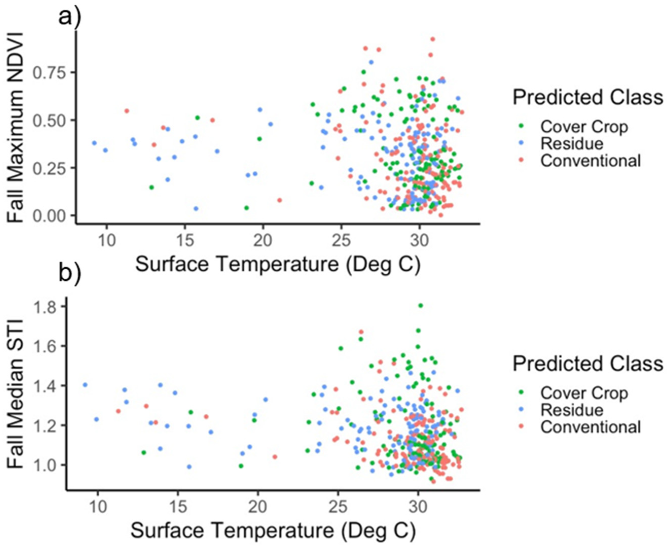
Variable importance scores for both the two- and three-class models showed that surface temperature was the most important predictive variable for both models (

Table 8. Variable importance scores for the two-class cover crop presence/absence and three-class cover crop/residue/bare soil model, ranked from most to least important. All metrics are the median fall observations (1 October—1 December) unless otherwise noted. More information on specific metrics can be found in Table 2. Displayed variable importance scores are scaled mean decrease accuracy (%IncMSE divided by its standard deviation).

Two-Class Model		Variable Importance	Three-Class Model
ST	100	Most Important	ST	100
STI	68.9		STI	82.8
B10-fullmax	57.4		NDTI	74.0
NDTI	54.0		B10_fullmax	69.2
NDVI-min	54.0		NDVI_med	59.8
NDVI-med	53.9		NDVI_min	46.8
NDVI-max	47.0		NDVI-mean	40.1
NDVI-fullmax	30.5		NDVI-max	39.0
NDVI-mean	29.2		B6	38.2
NDVI-amp	28.6		NDVI_fullmax	36.0
NDVI_ratio	25.5		NDVI_amp	31.9
B6	25.2		NDVI-ratio	31.3
Elapsed Days	24.6		B5	24.8
B10	20.3		Therm-Ratio	22.5
B5	19.9		B10	21.0
Therm_ratio	19.6		Elapsed Days	15.7
B3	10.7		B3	8.8
B9	0	Least Important	B9	0

). For the two-class model that predicted cover crop presence/absence, the standardized tillage index was the second most important, with a variable importance score of 68.9, followed by the annual maximum value of band B10 at 57.4 (Table 8). For the three-class model that predicted crop residues and cover crop presence, the STI and NDTI were the second and third most important variables, with variable importance scores of 82.8 and 74.0, respectively. (Table 8). Notably, ‘elapsed days’ were not highly important in either model, with scores of 24.6 and 15.6 for the two- and three-class models, respectively. Variability in ST and variability in fall maximum NDVI were not strongly coupled, (Figure 4a), underscoring the limited predictive power of NDVI in our classification models. There was stronger coupling between ST and STI, particularly for the cover crop class (Figure 4b). This suggests that the relationship between ST and STI may be useful in identifying cover crops.

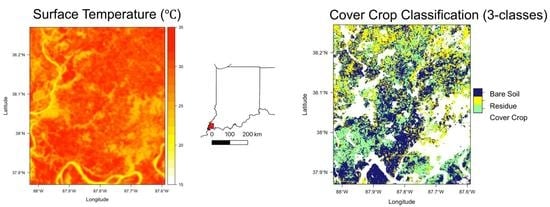
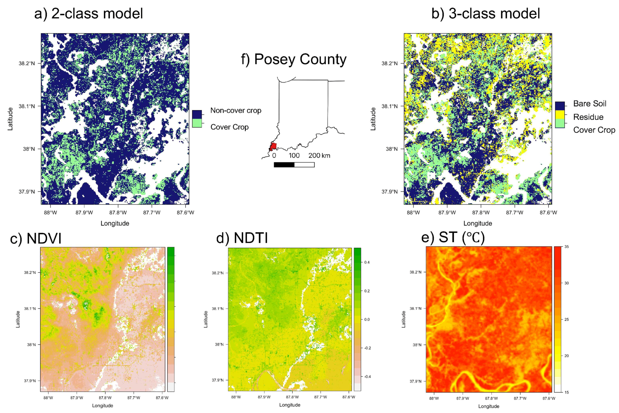
Despite high positive-class accuracy, the two-class model indicated a lower percentage of cover crops over Posey County than estimates from the Indiana Conservation Partnership (Figure 5). Cover crop presence is 24.8% in the two-class model, and 30.0% in the three-class model (Figure 5a,b). In the three-class model, there was also 25.0% crop residue coverage. Corresponding input variables are also plotted alongside random forest model results (Figure 5c–e).

4. Discussion

Our study evaluated the capacity of indices in the visible, NIR, SWIR, and thermal regions to predict winter cover crops and crop residues over the state of Indiana. Overall, we found that NDVI and metrics based solely on visible and NIR were not sufficient to detect cover crops or crop residues in Midwest agroecosystems. Our approach relied on comparing models with varying degrees of complexity by starting with NDVI, then adding a suite of indices from the visible and near-infrared, then incorporating SWIR bands, and finally incorporating thermal surface temperature data. For both our two- and three-class model, we found that a more complex model that included ST yielded the most accurate predictions of both cover crops and crop residues. Our work supports findings elsewhere in the literature [21,23,24] that beyond greenness—that is, going beyond the visible range and infrared bands—is essential to improve the detection of winter cover crops.

Each region of the electromagnetic spectrum tested here—VisNIR, SWIR, and thermal—is related to different characteristics of vegetation and thus each provides unique information for detection. The visible and near-infrared wavelengths are proxies for leaf area index and photosynthetic activity [47,48]. Wavelengths in the SWIR target the water, cellulose, and lignin in non-photosynthetically active vegetation to distinguish it from bare soils [49,50]. ST, which until now has not been used to detect winter agricultural practices at regional scales, is a variable with multifaceted connections to vegetation activity that incorporates the impacts of both vegetation structure (i.e., surface roughness; [51]) and function (i.e., transpiration; [52]).

A crucial finding of our study is that going beyond greenness meaningfully improved model ability to predict cover crop and crop residue presence on the landscape. Overall, remote sensing of vegetation based on the traditional multispectral ‘greenness’ paradigm is not sufficient to detect cover crops at spatial and temporal scales relevant to land use and land cover change. The NDVI-only based models had poor predictive power (k ≤ 0.2; Table 5). Random forest models based on a suite of indices in the visible and near-infrared improved model performance, likely by leveraging variables relevant to both fall vegetation cover (i.e., Fall NDVI) and growing season crop performance (i.e., elapsed days, [24]). Indices in the SWIR were more important in the three-class vegetation model than the two-class model, likely because the three-class model had a specific category for crop residues which are most distinguishable by wavelengths in the SWIR (Table 8). Even so, the SWIR index STI was the second most important predictive variable in the two-class model (Table 8). Finally, the addition of ST led to the best models for both the two- and three-class models (Table 5).

A second key finding from our study is that incorporating thermal data alongside SWIR resulted in the best detection model. Although there is little difference in ST between bare soil, crop residues, and cover crops in the dormant season, there are consistent differences between land cover types in the fall that can be leveraged by detection algorithms (Figure 2). Thermal data improved detection accuracy over the SWIR model for the two-class model, increasing kappa from 0.67 to 0.72 (Table 5). For the three-class model, thermal data also led to increased predictive power, increasing kappa from 0.61 to 0.69 (Table 5). While this improvement may seem small, incorporating thermal data offers several important advantages that should be treated as crucial to future detection. As temperatures drop in the fall, bare soil is the coldest, while crop residues that blanket the land surface keep the land surface relatively warm (Figure 2). Cover crops are in the middle, with slightly warmer temperatures than bare soil [53], potentially due to increased surface roughness of vegetation or lower albedo if snow is present [54]. Thermal data was the most important predictor variable in the three-class model, which suggests that thermal data can amplify the differences between photosynthetically active and non-photosynthetically active vegetation. Overall, incorporating thermal data greatly improves our ability to detect cover crops in Midwest agricultural lands.

Our iterative random forest classification approach allowed us to evaluate the additional predictive value added by each additional wavelength region through a series of increasingly complex models. Furthermore, the variable importance scores of random forest inputs allowed us to evaluate the relative predictive power of explanatory variables (Table 8). In contrast to empirical approaches that test for correlations between biomass and vegetation indices, our machine learning approach allows prediction of cover crop presence on novel regions based solely on remotely sensed inputs. Assessment of variable importance scores indicates that surface temperature has strongest predictive power in both the two- and three-class model (Table 8). Indices in the SWIR were the second most important variables for both the two- and three-class models, underscoring the importance of SWIR for both cover crop detection and crop residue detection. Continuing to improve accuracy is essential given remote sensing’s potential future role in monitoring and contributing to public policies, such as carbon markets and incentives for conservation agriculture adoption.

Ongoing improvements in spaceborne sensors means that additional information beyond greenness can be leveraged for agricultural applications including cover crop detection. Full-waveform information from hyperspectral imaging spectroscopy could distinguish photosynthetically active vegetation from crop residues and bare soils, and also allow investigation of individual species that comprise winter cover crops. Additionally, the increasing availability of high-resolution thermal data, like those provided by the ECOsystem Spaceborne Thermal Radiometer Experiment on Space Station (ECOSTRESS) instrument aboard the International Space Station [55], allows for further exploration of the predictive power of thermal data for questions relating to agricultural land-use practices.

The improved ability to accurately detect cover crops, as well as crop residues, in farmlands provides a critical advantage in understanding the ecological effects of these practices on local and regional carbon, water, and energy cycles (e.g., [4,56]). Being able to link carbon sequestration, changes in crop biomass, and nutrient cycling means researchers will be better able to model the carbon and energy balance mitigation potential of sequestration benefits and improvements in nitrate retention resulting from cover crops.

5. Conclusions and Future Directions: Implications for Policy and Management

This study demonstrated the value of going beyond greenness for the detection of cover crop and crop residues, which have critical climate mitigation and broader ecological implications. Improved detection, even incremental above the promising advantages of incorporating SWIR bands, has important policy and management implications for agriculture. As policymakers look towards additional mechanisms to encourage greater adoption of cover crops to promote carbon sequestration, such as carbon markets [57], the availability of reliable detection methods will be critical to advancing these opportunities as a monitoring tool. The availability of improved detection will also enable better trend analysis that can benefit farmers by identifying how cover crops affect cash crop yields, soil moisture and nitrogen fertilizer retention, and soil organic matter. These opportunities are crucial because farmers in the US Midwest have been slow to adopt zero tillage practices, which leave crop residues on the land surface, and slower still to adopt cover crops [9,58].

The rapid development of improved remote sensing of cover crops and crop residues has shown that relying solely on NDVI to detect cover crops is problematic because once winter cover crops become dormant, it is very difficult to distinguish between cover crops, crop residues, and bare soils that have significantly different ecological benefits but are highly intermixed. Incorporating SWIR bands and thermal data are both important to advancing remote sensing detection of agroecosystems, particularly as sensors improve and provide for more temporally and spatially refined resolutions, which will be very important to account for the variability in management decisions around the timing of planting and termination of cover crops. Thermal data could increase in importance as warming temperatures and changing precipitation patterns facilitate unexpected ecological and managerial responses [59]. Random forest classification is also crucial for prediction on novel data and model interpretability. This work was limited to only five counties in one Midwest US State and looked at fall cover crops only because of the available transect data.

Looking forward, better remote sensing detection of cover crops has the potential to be of critical importance to environmental management and policy. Cover crops are implicated in mitigating water pollution, climate adaption from improved soil moisture retention, climate mitigation through carbon sequestration, and increasing agrobiodiversity by expanding current crop rotations [2,4]. Improving the temporal and spatial resolution of cover crop detection will contribute to more comprehensive analysis of benefits of cover crops from local to regional scales and inform both agricultural and environmental management.

References

- Pielke, R.A.; Marland, G.; Betts, R.A.; Chase, T.N.; Eastman, J.L.; Niles, J.O.; Niyogi, D.D.S.; Running, S.W. The influence of Land-use change and landscape dynamics on the climate system: Relevance to climate-change policy beyond the radiative effect of greenhouse gases. Philos. Trans. R. Soc. Lond. Ser. A Math. Phys. Eng. Sci. 2002, 360, 1705–1719. [Google Scholar] [CrossRef] [PubMed]
- Lal, R. Soil carbon sequestration and aggregation by cover cropping. J. Soil Water Conserv. 2015, 70, 329–339. [Google Scholar] [CrossRef]
- Knowler, D.; Bradshaw, B. Farmers’ adoption of conservation agriculture: A review and synthesis of recent research. Food Policy 2007, 32, 25–48. [Google Scholar] [CrossRef]
- Kaye, J.P.; Quemada, M. Using cover crops to mitigate and adapt to climate change. A review. Agron. Sustain. Dev. 2017, 37, 1–17. [Google Scholar] [CrossRef]
- Feng, Z.; Leung, L.R.; Hagos, S.; Houze, R.A.; Burleyson, C.D.; Balaguru, K. More frequent intense and long-lived storms dominate the springtime trend in central US rainfall. Nat. Commun. 2016, 7, 13429. [Google Scholar] [CrossRef] [Green Version]
- Arbuckle, J.G.; Roesch-McNally, G. Cover crop adoption in Iowa: The role of perceived practice characteristics. J. Soil Water Conserv. 2015, 70, 418–429. [Google Scholar] [CrossRef] [Green Version]
- Montgomery, D.R. Growing a Revolution Bringing Our Soil Back to Life; WW Norton & Company: New York, NY, USA, 2018; ISBN 978-0-393-35609-0. [Google Scholar]
- Moyer, J.; Smith, A.; Rui, Y.; Hayden, J. Regenerative Agriculture and the Soil Carbon Solution. Available online: https://rodaleinstitute.org/wp-content/uploads/Rodale-Soil-Carbon-White-Paper_v11-compressed.pdf (accessed on 15 May 2021).
- USDA National Agriculture Statistics Service 2017 Census of Agriculture. Available online: https://www.nass.usda.gov/Publications/AgCensus/2017/index.php (accessed on 11 November 2020).
- Prabhakara, K.; Hively, W.D.; McCarty, G.W. Evaluating the relationship between biomass, percent groundcover and remote sensing indices across six winter cover crop fields in Maryland, United States. Int. J. Appl. Earth Obs. Geoinf. 2015, 39, 88–102. [Google Scholar] [CrossRef] [Green Version]
- Hively, W.D.; Duiker, S.; McCarty, G.; Prabhakara, K. Remote sensing to monitor cover crop adoption in southeastern Pennsylvania. J. Soil Water Conserv. 2015, 70, 340–352. [Google Scholar] [CrossRef] [Green Version]
- Thieme, A.; Yadav, S.; Oddo, P.C.; Fitz, J.M.; McCartney, S.; King, L.; Keppler, J.; McCarty, G.W.; Hively, W.D. Using NASA earth observations and google earth engine to map winter cover crop conservation performance in the Chesapeake Bay watershed. Remote Sens. Environ. 2020, 248, 111943. [Google Scholar] [CrossRef]
- Hunt, E.R.; Hively, W.D.; McCarty, G.W.; Daughtry, C.S.T.; Forrestal, P.J.; Kratochvil, R.J.; Carr, J.L.; Allen, N.F.; Fox-Rabinovitz, J.R.; Miller, C.D. NIR-green-blue high-resolution digital images for assessment of winter cover crop biomass. GISci. Remote Sens. 2011, 48, 86–98. [Google Scholar] [CrossRef]
- Skakun, S.; Franch, B.; Vermote, E.; Roger, J.-C.; Becker-Reshef, I.; Justice, C.; Kussul, N. Early season large-area winter crop mapping using MODIS NDVI data, growing degree days information and a gaussian mixture model. Remote Sens. Environ. 2017, 195, 244–258. [Google Scholar] [CrossRef]
- Gao, F.; Anderson, M.C.; Hively, W.D. Detecting cover crop end-of-season using VENµS and sentinel-2 Satellite imagery. Remote Sens. 2020, 12, 3524. [Google Scholar] [CrossRef]
- Atzberger, C.; Rembold, F. Mapping the spatial distribution of winter crops at sub-pixel level using AVHRR NDVI time series and neural nets. Remote Sens. 2013, 5, 1335–1354. [Google Scholar] [CrossRef] [Green Version]
- Hively, W.D.; Lang, M.; McCarty, G.W.; Keppler, J.; Sadeghi, A.; McConnell, L.L. Using satellite remote sensing to estimate winter cover crop nutrient uptake efficiency. J. Soil Water Conserv. 2009, 64, 303–313. [Google Scholar] [CrossRef] [Green Version]
- Natural Resources Conservation Service (NRCS) Cover Crop-Planting Specification Guide-NH-340 2011. Available online: https://www.nrcs.usda.gov/Internet/FSE_DOCUMENTS/stelprdb1081555.pdf (accessed on 15 November 2020).
- Hagen, S.C.; Delgado, G.; Ingraham, P.; Cooke, I.; Emery, R.; Fisk, J.P.; Melendy, L.; Olson, T.; Patti, S.; Rubin, N.; et al. Mapping conservation management practices and outcomes in the corn belt using the operational tillage information system (OpTIS) and the denitrification–decomposition (DNDC) model. Land 2020, 9, 408. [Google Scholar] [CrossRef]
- Bannari, A.; Staenz, K.; Champagne, C.; Khurshid, K.S. Spatial variability mapping of crop residue using hyperion (EO-1) hyperspectral data. Remote Sens. 2015, 7, 8107–8127. [Google Scholar] [CrossRef] [Green Version]
- Sonmez, N.K.; Slater, B. Measuring intensity of tillage and plant residue cover using remote sensing. Eur. J. Remote Sens. 2016, 49, 121–135. [Google Scholar] [CrossRef] [Green Version]
- Serbin, G.; Daughtry, C.S.T.; Hunt, E.R.; Reeves, J.B.; Brown, D.J. Effects of soil composition and mineralogy on remote sensing of crop residue cover. Remote Sens. Environ. 2009, 113, 224–238. [Google Scholar] [CrossRef]
- Hively, W.D.; Lamb, B.T.; Daughtry, C.S.T.; Shermeyer, J.; McCarty, G.W.; Quemada, M. Mapping crop residue and tillage intensity using WorldView-3 satellite shortwave infrared residue indices. Remote Sens. 2018, 10, 1657. [Google Scholar] [CrossRef] [Green Version]
- Seifert, C.A.; Azzari, G.; Lobell, D.B. Satellite detection of cover crops and their effects on crop yield in the midwestern United States. Environ. Res. Lett. 2018, 13, 064033. [Google Scholar] [CrossRef]
- Quemada, M.; Hively, W.D.; Daughtry, C.S.T.; Lamb, B.T.; Shermeyer, J. Improved crop residue cover estimates obtained by coupling spectral indices for residue and moisture. Remote Sens. Environ. 2018, 206, 33–44. [Google Scholar] [CrossRef]
- Hively, W.D.; Lee, S.; Sadeghi, A.M.; McCarty, G.W.; Lamb, B.T.; Soroka, A.M.; Keppler, J.; Yeo, I.-Y.; Moglen, G.E. Estimating the effect of winter cover crops on nitrogen leaching using cost-share enrollment data, satellite remote sensing, and soil and water assessment tool (SWAT) modeling. J. Soil Water Conserv. 2020, 75, 362375. [Google Scholar] [CrossRef]
- Fan, X.; Vrieling, A.; Muller, B.; Nelson, A. Winter cover crops in Dutch maize fields: Variability in quality and its drivers assessed from multi-temporal sentinel-2 imagery. Int. J. Appl. Earth Obs. Geoinf. 2020, 91, 102139. [Google Scholar] [CrossRef]
- Khanal, S.; Fulton, J.; Shearer, S. An overview of current and potential applications of thermal remote sensing in precision agriculture. Comput. Electron. Agric. 2017, 139, 22–32. [Google Scholar] [CrossRef]
- Sun, L.; Schulz, K. The improvement of land cover classification by thermal remote sensing. Remote Sens. 2015, 7, 8368–8390. [Google Scholar] [CrossRef] [Green Version]
- Sims, D.A.; Rahman, A.F.; Cordova, V.D.; El-Masri, B.Z.; Baldocchi, D.D.; Bolstad, P.V.; Flanagan, L.B.; Goldstein, A.H.; Hollinger, D.Y.; Misson, L.; et al. A new model of gross primary productivity for north American ecosystems based solely on the enhanced vegetation index and land surface temperature from MODIS. Remote Sens. Environ. 2008, 112, 1633–1646. [Google Scholar] [CrossRef]
- Jang, J.-D.; Viau, A.A.; Anctil, F. Thermal-water stress index from satellite images. Int. J. Remote Sens. 2006, 27, 1619–1639. [Google Scholar] [CrossRef]
- Gerhards, M.; Schlerf, M.; Mallick, K.; Udelhoven, T. Challenges and future perspectives of multi-/hyperspectral thermal infrared remote sensing for crop water-stress detection: A review. Remote Sens. 2019, 11, 1240. [Google Scholar] [CrossRef] [Green Version]
- Cook, M.; Schott, J.R.; Mandel, J.; Raqueno, N. Development of an operational calibration methodology for the landsat thermal data archive and initial testing of the atmospheric compensation component of a land surface temperature (LST) product from the archive. Remote Sens. 2014, 6, 11244–11266. [Google Scholar] [CrossRef] [Green Version]
- FAOSTAT. Available online: http://www.fao.org/faostat/en/#data/QC (accessed on 5 May 2021).
- Agriculture in the Midwest|USDA Climate Hubs. Available online: https://www.climatehubs.usda.gov/hubs/midwest/topic/agriculture-midwest (accessed on 5 May 2021).
- Mannering, J.V.; Griffith, D.R.; Johnson, K.D. Winter Cover Crops—Their Value and Management. Available online: https://www.agry.purdue.edu/Ext/forages/rotational/articles/PDFs-pubs/winter-cover-crops.pdf (accessed on 15 May 2021).
- ISDA Cover Crop and Tillage Transect Data. Available online: https://www.in.gov/isda/divisions/soil-conservation/cover-crop-and-tillage-transect-data (accessed on 5 May 2021).
- Claverie, M.; Ju, J.; Masek, J.G.; Dungan, J.L.; Vermote, E.F.; Roger, J.-C.; Skakun, S.V.; Justice, C. The harmonized landsat and sentinel-2 surface reflectance data set. Remote Sens. Environ. 2018, 219, 145–161. [Google Scholar] [CrossRef]
- Bivand, R.; Keitt, T.; Rowlingson, B.; Pebesma, E.; Sumner, M.; Hijmans, R.; Rouault, E.; Bivand, M.R. Package ‘Rgdal.’ Bindings for the Geospatial Data. Abstraction Library. Available online: https://cran.r-project.org/web/packages/rgdal/index.html (accessed on 15 October 2020).
- Team, R.C. R: The R Project for Statistical Computing. 2019. Available online: https://www.r-project.org/ (accessed on 30 March 2020).
- Claverie, M.; Masek, J.G.; Ju, J.; Dungan, J.L. Harmonized Landsat-8 Sentinel-2 (HLS) Product User’s Guide; National Aeronautics and Space Administration (NASA): Washington, DC, USA, 2017.
- Hively, W.D.; Shermeyer, J.; Lamb, B.T.; Daughtry, C.T.; Quemada, M.; Keppler, J. Mapping crop residue by combining landsat and WorldView-3 satellite imagery. Remote Sens. 2019, 11, 1857. [Google Scholar] [CrossRef] [Green Version]
- Van Deventer, A.P.; Ward, A.D.; Gowda, P.H.; Lyon, J.G. Using thematic mapper data to identify contrasting soil plains and tillage practices. Photogramm. Eng. Remote Sens. 1997, 63, 87–93. [Google Scholar]
- Liaw, A.; Wiener, M. Classification and regression by randomForest. R News 2002, 2, 18–22. [Google Scholar]
- Kuhn, M. Building predictive models in R using the caret package. J. Stat. Soft. 2008, 28. [Google Scholar] [CrossRef] [Green Version]
- Landis, J.R.; Koch, G.G. An application of hierarchical kappa-type statistics in the assessment of majority agreement among multiple observers. Biometrics 1977, 33, 363–374. [Google Scholar] [CrossRef] [PubMed]
- Gamon, J.A.; Field, C.B.; Goulden, M.L.; Griffin, K.L.; Hartley, A.E.; Joel, G.; Penuelas, J.; Valentini, R. Relationships between NDVI, canopy structure, and photosynthesis in three Californian vegetation types. Ecol. Appl. 1995, 5, 28–41. [Google Scholar] [CrossRef] [Green Version]
- Carlson, T.N.; Ripley, D.A. On the relation between NDVI, fractional vegetation cover, and leaf area index. Remote Sens. Environ. 1997, 62, 241–252. [Google Scholar] [CrossRef]
- Asner, G.P.; Lobell, D.B. A biogeophysical approach for automated SWIR unmixing of soils and vegetation. Remote Sens. Environ. 2000, 74, 99–112. [Google Scholar] [CrossRef]
- Peña-Barragán, J.M.; Ngugi, M.K.; Plant, R.E.; Six, J. Object-based crop identification using multiple vegetation indices, textural features and crop phenology. Remote Sens. Environ. 2011, 115, 1301–1316. [Google Scholar] [CrossRef]
- Kalma, J.D.; McVicar, T.R.; McCabe, M.F. Estimating land surface evaporation: A review of methods using remotely sensed surface temperature data. Surv. Geophys. 2008, 29, 421–469. [Google Scholar] [CrossRef]
- Boegh, E.; Soegaard, H.; Hanan, N.; Kabat, P.; Lesch, L. A remote sensing study of the NDVI–Ts relationship and the transpiration from sparse vegetation in the Sahel based on high-resolution satellite data. Remote Sens. Environ. 1999, 69, 224–240. [Google Scholar] [CrossRef]
- Calkins, J.B.; Swanson, B.T. Comparison of conventional and alternative nursery field management systems: Soil physical properties. J. Environ. Hortic. 1998, 16, 90–97. [Google Scholar] [CrossRef]
- Lombardozzi, D.L.; Bonan, G.B.; Wieder, W.; Grandy, A.S.; Morris, C.; Lawrence, D.L. Cover crops may cause winter warming in snow-covered regions. Geophys. Res. Lett. 2018, 45, 9889–9897. [Google Scholar] [CrossRef]
- Hulley, G.; Hook, S.; Fisher, J.; Lee, C. ECOSTRESS, a NASA earth-ventures instrument for studying links between the water cycle and plant health over the diurnal cycle. In Proceedings of the 2017 IEEE International Geoscience and Remote Sensing Symposium (IGARSS), Fort Worth, TX, USA, 23–28 July 2017; pp. 5494–5496. [Google Scholar]
- Hanrahan, B.R.; Tank, J.L.; Christopher, S.F.; Mahl, U.H.; Trentman, M.T.; Royer, T.V. Winter cover crops reduce nitrate loss in an agricultural watershed in the central U.S. Agric. Ecosyst. Environ. 2018, 265, 513–523. [Google Scholar] [CrossRef]
- Thiele, R. Sen. Mike Braun’s Bill Could Help Reward Climate-Friendly Farmers. Available online: https://indianapublicradio.org/news/2020/06/sen-mike-brauns-bill-could-help-reward-climate-friendly-farmers/ (accessed on 12 April 2021).
- Lal, R.; Reicosky, D.C.; Hanson, J.D. Evolution of the plow over 10,000 years and the rationale for no-till farming. Soil Tillage Res. 2007, 93, 1–12. [Google Scholar] [CrossRef]
- Still, C.J.; Rastogi, B.; Page, G.F.M.; Griffith, D.M.; Sibley, A.; Schulze, M.; Hawkins, L.; Pau, S.; Detto, M.; Helliker, B.R. Imaging canopy temperature: Shedding (thermal) light on ecosystem processes. New Phytol. 2021, 230, 1746–1753. [Google Scholar] [CrossRef]
Figure 1.
Seasonal NDVI cycle for farm fields in Indiana, USA, with cover crops (green), crop residues (blue), and conventional tillage (bare soil-red) in the fall of 2015. Each line represents the aggregate cycle of six individual farm NDVI time series for each agricultural land use practice. The MOD13Q1 16-day, 250 m vegetation product point samples were obtained from the Application for Extracting and Exploring Analysis Ready Samples (AppEEARS Team, 2020).
Figure 2.
Autumn land surface temperatures (LST) for farm fields in Posey County with cover crops (green), crop residues (blue), and conventional tillage (bare soil-red) in the fall of 2015. Each line represents the aggregate cycle of six individual farm LST time series for each agricultural land use practice. The MOD11Q1 daily, 1 km daytime LST product point samples were obtained from the Application for Extracting and Exploring Analysis Ready Samples (AppEEARS Team, 2020).
Figure 3.
Counties in Indiana with cover crop/tillage survey data, overlain on winter NDVI from MODIS. Colors indicate the percentage of GPS points with fall cover crops in 2015 (out of all GPS points) per county. The total number of GPS points per county is also indicated.
Figure 4.
Scatter plots of ST against (a) fall maximum NDVI and (b) fall median STI in focal fields in Posey and Gibson counties. Points are colored by classified category (in the three-class model), with cover crops (green), crop residues (blue), and conventional tillage (bare soil-red).
Figure 5.
Results of cover crop estimation over portions of Indiana’s Posey county (f), which has the highest cover crop adoption rates in the state. Estimates based on the two-class cover crop presence/absence (a) and the three-class cover crop and crop residue (b) model are shown alongside key input variables: NDVI (c), the NDTI (d), and surface temperature (e).