
Monitoring the Structure of Regenerating Vegetation Using Drone-Based Digital Aerial Photogrammetry


1
Faculty of Forestry, University of British Columbia, Vancouver, BC V6T 1Z4, Canada
2
TC Energy, Calgary, AB T2P 5H1, Canada
*
Author to whom correspondence should be addressed.
Remote Sens. 2021, 13(10), 1942; https://doi.org/10.3390/rs13101942
Submission received: 3 April 2021
/
Revised: 8 May 2021
/
Accepted: 12 May 2021
/
Published: 16 May 2021
(This article belongs to the Special Issue Drones for Ecology and Conservation)
Abstract
:Measures of vegetation structure are often key within ecological restoration monitoring programs because a change in structure is rapidly identifiable, measurements are straightforward, and structure is often a good surrogate for species composition. This paper investigates the use of drone-based digital aerial photogrammetry (DAP) for the characterization of the structure of regenerating vegetation as well as the ability to inform restoration programs through spatial arrangement assessment. We used cluster analysis on five DAP-derived metrics to classify vegetation structure into seven classes across three sites of ongoing restoration since linear disturbances in 2005, 2009, and 2014 in temperate and boreal coniferous forests in Alberta, Canada. The spatial arrangement of structure classes was assessed using land cover maps, mean patch size, and measures of local spatial association. We observed DAP heights of short-stature vegetation were consistently underestimated, but strong correlations (rs > 0.75) with field height were found for juvenile trees, shrubs, and perennials. Metrics of height and canopy complexity allowed for the extraction of relatively tall and complex vegetation structures, whereas canopy cover and height variability metrics enabled the classification of the shortest vegetation structures. We found that the boreal site disturbed in 2009 had the highest cover of classes associated with complex vegetation structures. This included early regenerative (22%) and taller (13.2%) wood-like structures as well as structures representative of tall graminoid and perennial vegetation (15.3%), which also showed the highest patchiness. The developed tools provide large-scale maps of the structure, enabling the identification and assessment of vegetational patterns, which is challenging based on traditional field sampling that requires pre-defined location-based hypotheses. The approach can serve as a basis for the evaluation of specialized restoration objectives as well as objectives tailored towards processes of ecological succession, and support prioritization of future inspections and mitigation measures.

1. Introduction
Global demand for natural resources such as natural gas and minerals is expected to continue to grow in the next two decades [1,2] which in turn has ongoing implications for biodiversity and ecosystem functions in forest ecosystems [3]. Forest disturbances associated with these anthropogenic activities have been shown to be drivers of alien species invasion, changing soil stability including erosion and compaction, groundwater storage, water flow, and landscape fragmentation [3,4,5]. Forest restoration activities, which involve reestablishing biodiversity and ecological processes on disturbed sites to accelerate forest recovery, have been successful in offsetting or minimizing the impacts of industrial activities and developments, including mines, seismic lines, and roads [6,7]. As a result, there is a growing interest in mandatory restoration policies, some of which have been implemented by industry in the last decade [8,9,10].
Restoration goals and objectives must be set in order to evaluate restoration success. These can be unambiguous, such as the implementation of quick erosion control, improving water quality, or limiting invasion of alien species, or more complex and holistic when focused on restoring ecological processes and biodiversity towards a resilient state [11]. Theory-driven reference targets can be developed in line with project goals that combine knowledge about ecological principles, present-day reference sites, on-the-ground restoration experience, and historical records [12,13,14]. To be able to evaluate success, a set of indicators should be developed that reflect restoration objectives, are easy to measure, have a known response to stresses in the ecosystem and ecological succession, and can be linked to management actions [15].
In terrestrial ecosystems, quantitative indicators that capture vegetation structure are commonly used, e.g., cover by vertical stratum, cover by life form, and canopy height [16]. Vegetation structure is relatively static, efficient, and rapid to measure, and has been associated with successional stages [16]. It can also be used as an indirect indicator for processes such as controlling erosion or improving water quality [11]. The spatial arrangement, patterns, and patchiness of vegetation structure can be associated with topography and ecological processes across spatial, temporal, and thematic scales [17] and as a result, provide insights into recovery patterns [18].
Measuring forest structure, however, especially of short-stature vegetation over large areas that have undergone disturbance, is difficult and constrained by resources (e.g., time, costs, and expertise). Traditional field sampling is typically undertaken manually using quadrats positioned with Global Navigation Satellite Systems (GNSS) which is demanding on project resources especially when large, remote, or hazardous areas need to be covered [19]. In addition, it is challenging to define spatial, temporal, and thematic scales at which monitoring is carried out, resulting in trade-offs and indicators not being well-aligned with restoration objectives as well as processes of ecological succession [18,20].
Remote sensing, in combination with geospatial data analysis techniques, can be used to provide spatially continuous, i.e., wall-to-wall, measurements of vegetation structure. Currently, a range of remote sensing sensors and platforms exist that allow the characterization and mapping of vegetation structure at scales previously unavailable to ecologists and restoration professionals. Relevant remote-sensing technologies include Light Detection and Ranging (LiDAR, i.e., laser scanning) and structure-from-motion photogrammetry, which can be deployed from manned or unmanned aerial systems (drones), spaceborne systems, tripods, or movable handheld devices [17,21,22]. Airborne LiDAR, i.e., airborne laser scanning (ALS) data are increasingly available, partly due to joint public–private campaigns reducing acquisition costs, providing opportunities for characterizing vertical and horizontal vegetation structure over large areas [22]. Digital aerial photogrammetry (DAP) utilizes conventional or multispectral cameras, structure-from-motion photogrammetry, and accurate GNSS measurements (typically including ground-control-points) to reconstruct detailed three-dimensional surfaces, represented as point clouds, meshes, or digital surface models, from sequences of photographs with high spatial overlap. Increasing computing power, automated and simplified processing workflows, development of open-source software, and decreasing computer costs are making DAP increasingly accessible for ecological monitoring [23,24]. Critically, DAP can be acquired by drones which have been shown to be able to acquire information about vegetation structure at reduced costs, more frequent intervals, and higher spatial resolutions compared to airborne and spaceborne platforms. The advantages of DAP reconstructions are their high level-of-detail and the ability to incorporate spectral information [25,26,27]. Unlike ALS, drone-based DAP primarily characterizes the outer canopy envelope [28], limiting the ability to accurately model terrain which is a prerequisite for measuring vegetation height. Despite this, others have shown that DAP is capable of characterizing the structure of small plants depending on vegetation density, the slope of the terrain, careful ground filtering, and implemented geometric control [25,26,29,30,31].
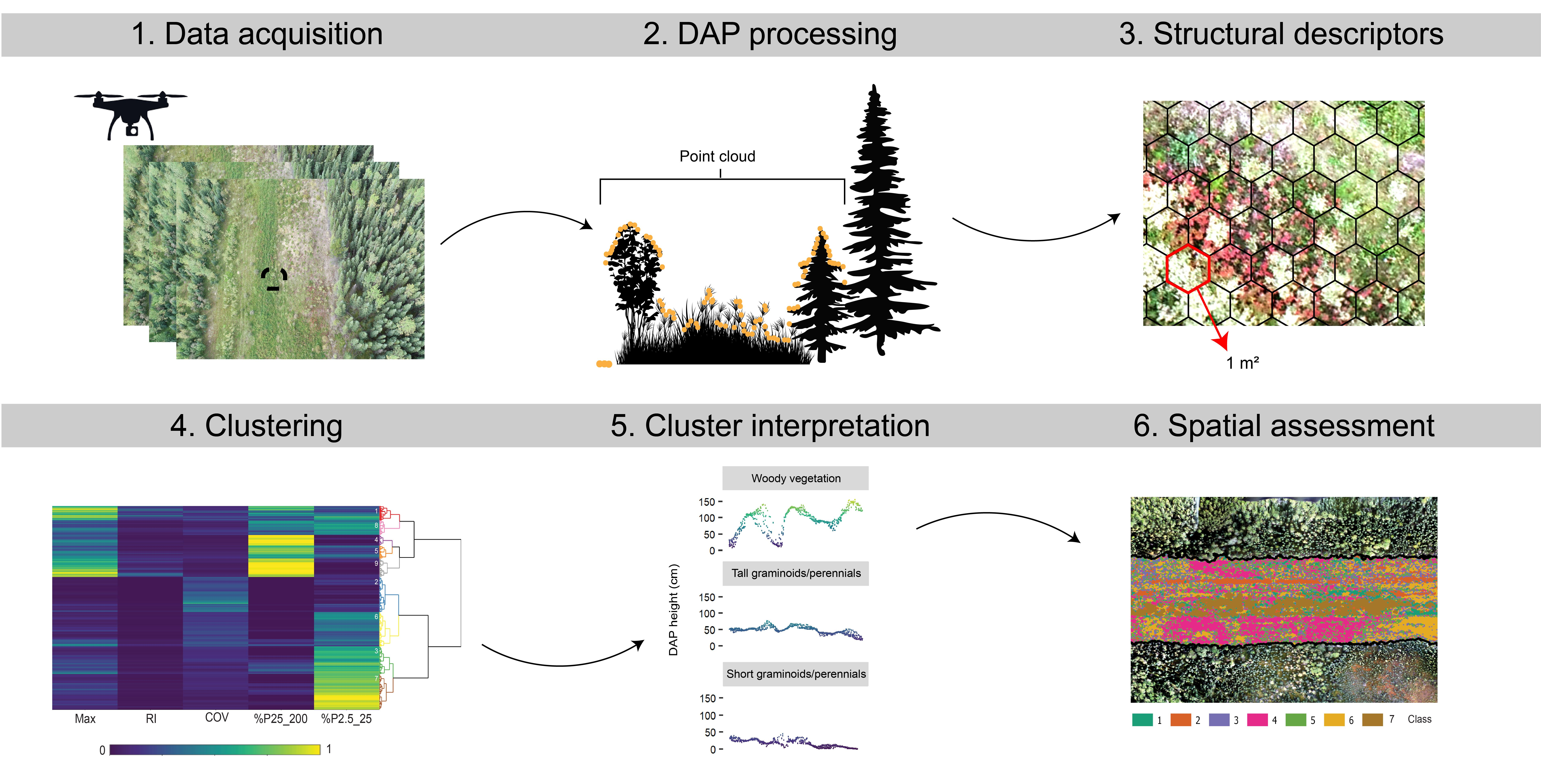
In this study, we examine the capacity of DAP-based vegetation structure metrics, acquired by a drone, to map classes of regenerating vegetation structure to inform ecological management and restoration. DAP data were acquired on three natural gas pipeline rights-of-ways (ROWs) in northwest Alberta, Canada. First, DAP-derived vegetation heights were compared to in situ heights of various vegetation life forms. Second, vegetation structure metrics were calculated over a regularized surface over the ROW, representing vegetation cover, vegetation height, height distribution, variability, and surface complexity. Classes of structure were then developed using a two-stage clustering analysis and patterns of structure were evaluated across sites using indicators of local spatial associations. Understanding the capacity of rapidly deployed DAP datasets to characterize short-stature vegetation structure (i.e., <2 m) within environments with high complexity and variability of vegetation cover is important, as timely mitigation measures are desired within these areas of ongoing anthropogenic disturbance. Similarly, the developed workflow aims to inform users of these data of potential in these applications.
2. Materials and Methods
2.1. Research Context: Pipeline Operations, Restoration, and Monitoring
The Province of Alberta is a key producer of oil and gas production within Canada, and the 4th largest producer of oil and natural gas worldwide, representing 81% and 64% of Canada’s total oil and gas production, respectively [32,33]. The production is characterized by the development of a complex network of seismic lines, roads, and pipelines and other infrastructure, e.g., wells and oil sands [34]. The infrastructural networks can have ecological implications for both plant and animal biodiversity and as a result, operators and regulators aim to reduce their impact on the landscape. This includes implementing reclamation and monitoring frameworks [5,35,36,37,38]. Pipelines are typically constructed underground (0.8 to 2 m depth) requiring a 15 to 30 m wide ROW [39,40]. Since the early 2000s, pipeline construction in Alberta uses minimal surface disturbance (MSD) construction practices, where possible, to reduce their overall construction footprint. MSD techniques where root layers and seedbed sources are left largely undisturbed, lay the foundation for natural regeneration and rapid re-establishment of planted vegetation on pipeline ROWs. MSD techniques during construction can be achieved by mulching in the ROW during frozen conditions to reduce disturbance of surface soils except where grading is necessary, limiting the size of machinery used, and using heavy machinery only on frozen soils or rig mats [40,41,42].
The industry is required to develop environmental protection plans associated with regeneration of native vegetation (e.g., minimizing soil disturbance, seeding, and weed management), erosion control, access management (e.g., limiting public access and minimizing the footprint of access routes on ROW) and when in caribou range, provide provincially required Woodland Caribou (Rangifer tarandus caribou) protection plans (e.g., breaking line-of-sight for predators) [43,44,45]. Post-construction monitoring is performed to confirm the effectiveness of environmental protection and mitigation measures. Objectives include, among others, monitoring of drainage patterns (e.g., erosion and stream bank stability), assessment of total live cover on the ROW versus off-ROW, assessment of wetland-specific species composition, and identification of undesirable species as defined under the Alberta Weed Control Act [46,47]. In Woodland Caribou range, there may be federal requirements, depending upon the project approval conditions, to assess line-of-sight, seedling density, species richness, and composition of general life forms including lichen, moss, graminoids, herbaceous, shrubs, and trees according to three general ecosite types: non-wetland forests, treed, and non-treed wetlands [38].
2.2. Study Sites
Across the region, we selected three sections on ROWs which are part of an extensive natural gas transmission pipeline system and which covered a range of ecosites and ages of pipeline construction. Details are summarized in Table 1 including ecoregion, elevation, aspect, construction year, and area of image acquisition. To include a range of different ecosite conditions, we focused on two Natural Regions and Subregions [48], the Lower Boreal Highlands and Upper Foothills, and located sites with a close proximity to roads (for field and drone control access) representing a variety of slopes and elevations.
The Lower Boreal Highlands are characterized by extensive wetlands within flat areas and mixedwood forests on slopes of hill systems, whereas a more diverse complex of conifer, deciduous, and mixedwood forest stands as well as fens and shrubby grasslands characterize the Upper Foothills region. Elevations in the Lower Boreal Highlands range from 400 to 1075 m. Mixedwood forests are found on moist slopes and include aspen poplar (Populus tremuloides), balsam poplar (Populus balsamifera), black spruce (Picea mariana), white spruce (Picea glauca), white birch (Betula papyrifera), or hybrids between lodgepole pine (Pinus contorta) and jack pine (Banksiana) [48,49]. Extensive wetlands are found on level sites and are typically treed, shrubby, or graminoid fens. Within the Chinchaga Plain, which is south of the two study sites in the Lower Boreal region, the bog wetland type makes up almost 50% of total wetland cover [48]. The Upper Foothills region, with elevations ranging between 950 and 1750 m, is typically dominated by conifer forest stands including lodgepole pine, black spruce, and white spruce [49]. Deciduous and mixedwood stands occur on south and west-facing slopes. Poor-to-rich fens occur in valleys and shrubby grasslands on the driest sites [48].
2.3. In Situ Measurements
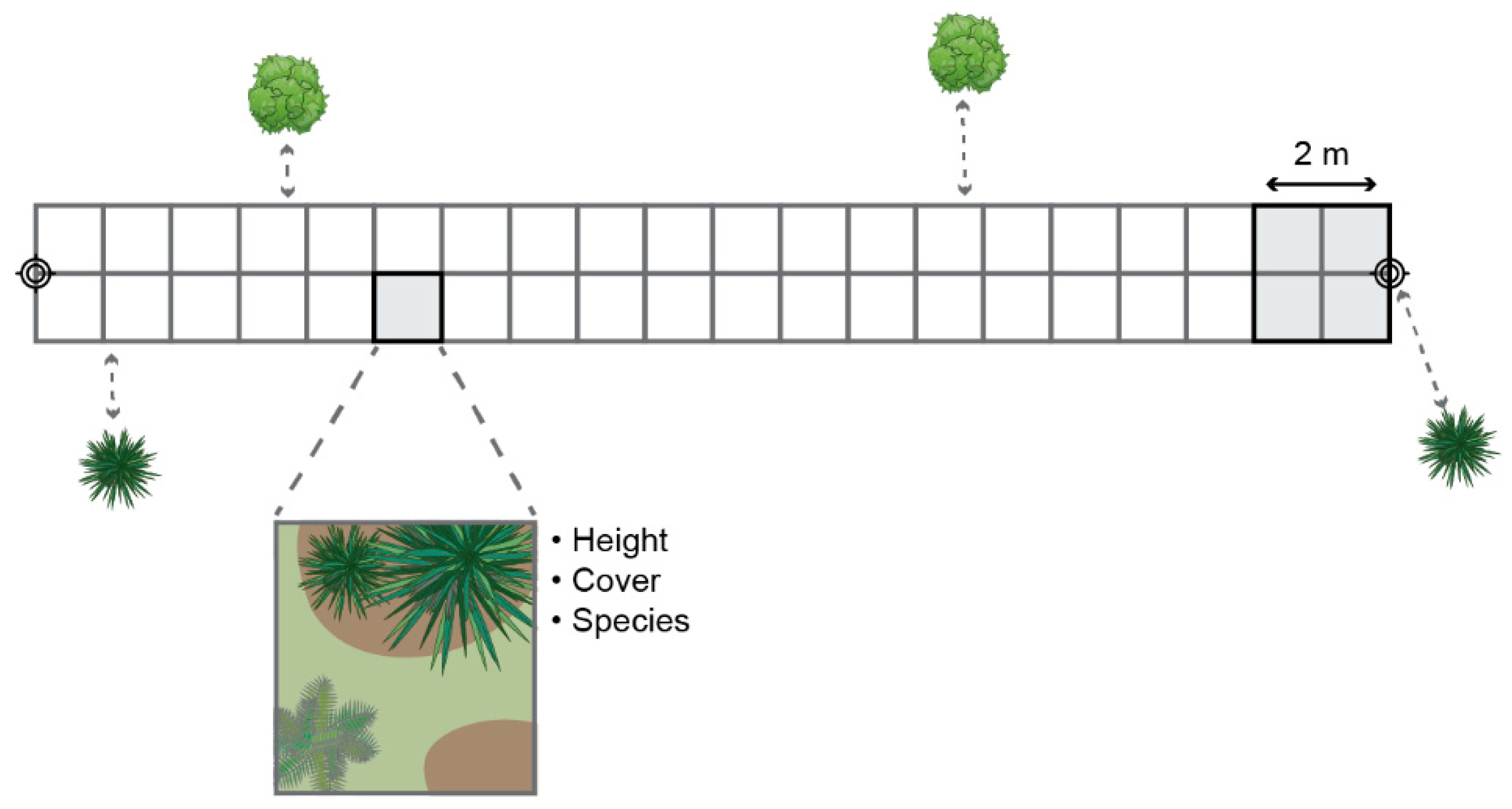
Vegetation height and structure on the ROW were sampled across seven transects at each of the three study sites. It was hypothesized that transects, placed perpendicular to the pipelines, would best represent species diversity, as they may cross sections with various soil and illumination, as well as underground infrastructure. All field samples were collected in August 2019. Transect locations were determined in the field based on an optimal representation of vegetation type diversity visually observed at each study site. Start and end locations of each transect were recorded using a Trimble Geo7X ground station, which were post-processed using differential GNSS data of a station in Fort Saint John, British Columbia. Each transect consisted of 40 1 x 1 m2 cells, as shown in Figure 1. Within each cell, maximum height, cover percentage, and associated species were recorded. A species was not recorded when it covered less than 10% of the cell. To verify transect alignment with the acquired imagery, locations of known neighboring trees or large shrubs were used. Additionally, up to 300 terrestrial photographs were taken along each transect as a reference.
It was anticipated that lower stature vegetation would show little structural variation in the DAP reconstructions and that heights derived from DAP datasets would be underestimated [26,29,50]. Therefore, in situ measurements and clustering, which are described in Section 2.5.4, were limited to heights up to 2 m potentially improving the capability to distinguish the shortest life forms from DAP such as grasses and perennials. The observed plant species are listed in Table 2, including representative life form and study site(s) of occurrence. Species identification was limited to conifer and deciduous trees, shrubs, perennials (both herbaceous and woody), and weeds listed under Alberta’s Weed Control Act [51]. Cover percentages and, if applicable, heights of graminoids, mosses, or bare soil were recorded, however, graminoids were only identified as short- or tall-growing (rushes and sedges) graminoids and moss species were not identified.
2.4. Data Acquisition and Photogrammetric Processing
Imagery from three drone flights was acquired in August and September 2019 using a 20-megapixel camera, measuring in red, green, and blue, carried by a DJI Phantom 4 Pro (integrated camera) or DJI Matrice 200 v2 (Zenmuse X5S camera) system. Drones include a ground control station with integrated flight planning software, collision avoidance systems, and IMU and GPS units, allowing for semi-autonomous data collection. Mean flying height, overlap, and weather conditions varied between the three data acquisitions. Table 3 summarizes flight parameters, conditions, and data specifications. High height above ground level (HAGL) was necessary to comply with visual line-of-sight requirements and to allow for rapid data collection. Overcast weather resulted in minimal shadowing at sites A and B, while sunny conditions resulted in heavy shadowing at site C. A pair of ground control points (GCPs) was placed on the ROW approximately every 200 m, resulting in a total of 4, 10, and 6 GCPs at site A, B, and C, respectively. GCPs were registered using a Real-Time Kinematic (RTK) GPS ground station and post-processed using a Precise Point Positioning (PPP) service.
Structure-from-motion photogrammetry was used to produce georectified wall-to-wall point clouds and orthomosaics [52]. The developed workflow incorporates a Scale-Invariant Feature Transform (SIFT) algorithm to locate conjugate tie-points between overlapping images, followed by a bundle block adjustment procedure that determines positions and altitudes of images in 3D space, incorporating GCPs and in-flight GPS and IMU measurements [53,54,55]. Following image alignment, orthomosaics and dense DAP point clouds were built with ground sample distances (GSDs) ranging between 1.6 and 1.95 cm/pixel and mean point densities between 885 and 1190 points m−2. Original image scales were used throughout all photogrammetric processing steps. Root mean square errors (RMSE) of the models of sites A and B were close to 1 cm in X, Y, and Z whereas RMSEs for site C were 34.4 (X), 34.8 (Y), and 7.8 (Z) cm.
2.5. Processing and Analysis
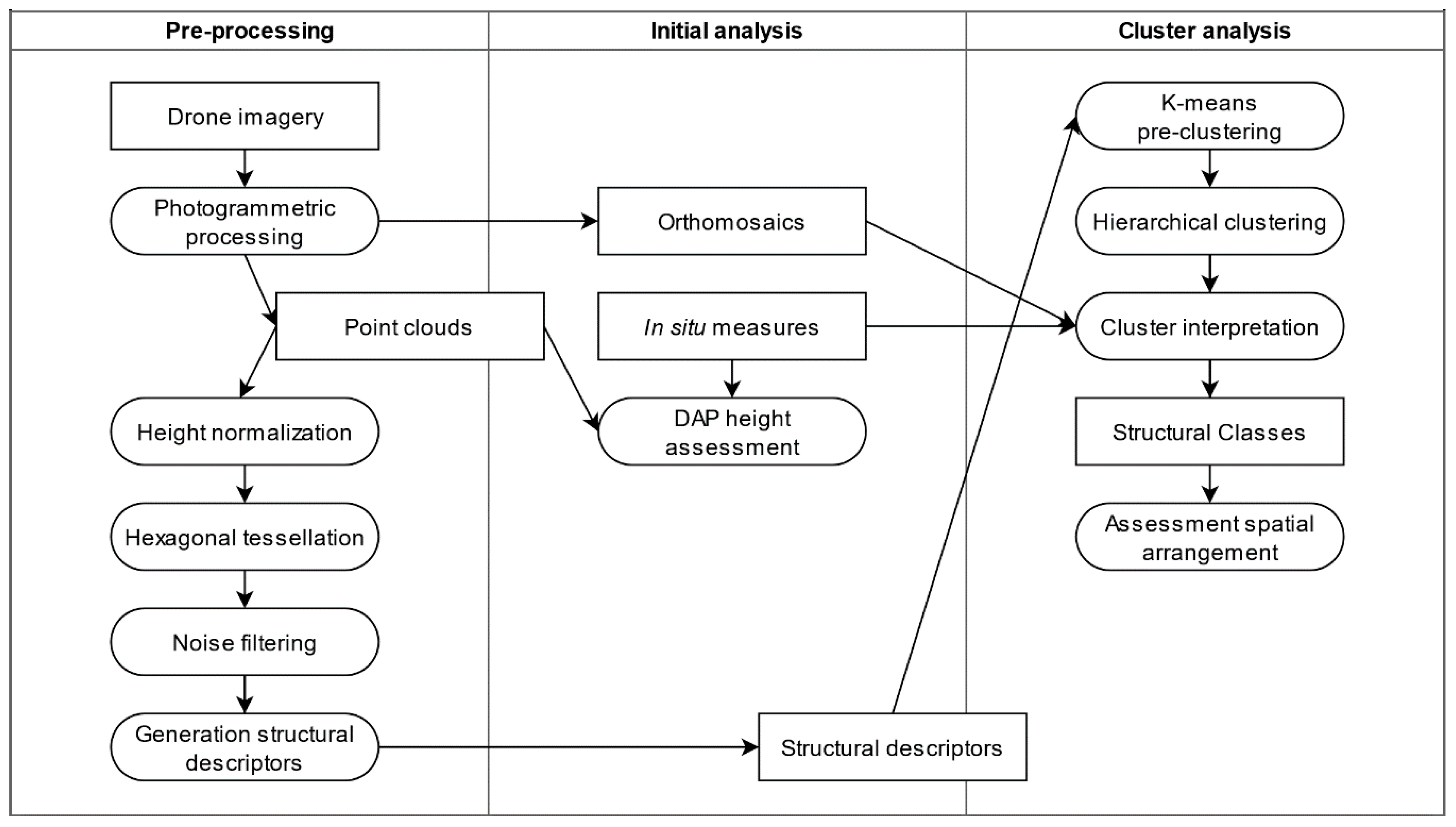
Processing and analysis comprised six steps: (1) point cloud post-processing including ground filtering and height normalization, (2) DAP height assessment, (3) generation of hexagon-based descriptions of structure, (4) clustering analysis, (5) cluster interpretation, and (6) assessment of arrangement of vegetation structure across the study sites. Figure 2 presents a methodological flow diagram and each processing step is described in detail below.
2.5.1. Point-Cloud Processing
Critical to the derivation of structure metrics, including vegetation heights, is the accurate definition of terrain which is especially important when focusing on lower-stature vegetation. Ground points were filtered conservatively in the DAP point clouds using triangulated irregular network (TIN) densification followed by an iterative surface lowering (ISL) method [56,57]. In short, the TIN densification method creates a sparse triangular surface model based on the lowest points within a search window, after which spikes are removed and points added iteratively based on certain criteria such as maximum distance away from the surface and angle [56,57]. Set parameters include step (5 m), spike (50 cm), offset (10 cm), and bulge (0°). The ISL refinement method was applied to remove ground points at the foot of bulges, i.e., mounds that may have been classified incorrectly. ISL uses ground points from TIN densification and iteratively removes points below a digital terrain model (DTM) created at each step using Delaunay triangulation.
Consistent point densities are required to derive point-based metrics of vegetation structure. Point densities vary between data acquisitions, as shown in Table 3, but also within each site depending on vegetation cover. Therefore, all point clouds were thinned after normalization, keeping only the highest point per 4 × 4 cm2. Since the focus of the analysis was short-stature vegetation (<2 m), an additional filtering step was undertaken to remove high points from overhanging branches.
2.5.2. DAP Height Assessment
To confirm that short-stature vegetation heights can be accurately reconstructed in the DAP point clouds, we investigated the relationship between in situ and DAP height, which was assessed by life form. First, the in situ heights measured along the transects were summarized into 2 × 2 m2 cells to reduce positioning errors. Second, for each 2-m cell the maximum DAP and in situ height were derived, stratified by life form, and compared using regression and Spearman correlation coefficients. In addition, mean height offsets (i.e., bias), root-mean-square errors (RMSEs), and normalized RMSEs, were calculated as described by [29].
2.5.3. Structure Metrics
Previous analysis of vegetation structure using DAP datasets has incorporated metrics describing the 3D point distribution, which are related to vegetation height, height variability, and canopy cover [58,59]. Most of these metrics have been shown to be representative of forest structure at the stand level, however, their applicability at finer spatial resolutions and for short-stature vegetation is less well demonstrated. We summarized the DAP point clouds using a hexagonal tessellation, with each hexagon being 1 m2, on the assumption that hexagons better represent natural vegetation features compared to a grid. The metrics derived within each 1 m2 hexagon are listed in Table 4 and were selected to describe key characteristics of vegetation structure.
High multicollinearity between height metrics, as well as reduced dispersion in height variability between different short vegetation types was anticipated. We also computed metrics of canopy surface complexity, the Rumple index, which represents the area of a canopy surface modeled using Delaunay triangulation divided by the area of a projected flat surface [60]. Metrics of point density, i.e., vegetation cover, by vertical height strata and variability were also calculated [61].
All metrics were tested for multicollinearity and removed from analysis if inter-correlation (r) > 0.8. Selected metrics include maximum height (Max), coefficient of variation (COV), Rumple index, percentage points between 2.5 and 25 cm (%P2.5_25), and total vegetation cover (%P25_200). Maximum height was preferred over percentile heights as it retains treetops. Principle Component Analysis (PCA) was performed on the initial hexagon-based summaries to analyze the distribution of variance across the selected metrics and assess their contribution to variance [62].
2.5.4. Two-Step Clustering Analysis
We clustered the selected metrics over the landscape to produce a classification of vegetation structure to inform restoration activities. Two-step clustering approaches have been shown to be highly effective on large remotely sensed datasets, [61,63,64], improving scalability and reducing computing times compared to conventional multivariate clustering by incorporating a pre-clustering method, in our case, the k-means++ algorithm [64]. As a result, agglomerative hierarchical clustering was performed to group the pre-clusters using the Ward linkage algorithm and Euclidian distance [65]. From the initial pre-clusters, an optimal number of clusters was defined by the gap statistic which compares total intra-cluster variation with a hypothetical distribution showing no natural grouping. The optimal number of clusters (k) is found where the gap statistic is maximized but k is minimized.
2.5.5. Cluster Comparison and Interpretation
To assess the uniqueness of the derived clusters, we performed Dunn’s post hoc multiple pairwise comparisons that evaluates, for each metric, whether clusters are significantly different [66,67]. In addition, exploratory data analysis through visualization was used to assess cluster characteristics, which included: a heatmap and dendrogram organized by hierarchical relations, boxplots of metrics, and cross-sections of the point clouds. Based on these assessments, similar clusters were merged to result in a final classification of structure. To interpret the indicative vegetation features and types in each cluster, such as a dominant life form, level of regeneration, or dominant species, we overlaid and assessed the seven transects.
2.5.6. Cover and Spatial Arrangement
Lastly, to demonstrate how class cover and spatial arrangement can be used to evaluate the state of regeneration, we summarized and mapped measures of local spatial association of the structure classes. To do so we utilized a novel entropy-based local indicator of spatial association (ELSA), introduced by [68], that can be applied to categorical data. We used a search radius of 3.3 m.
2.6. Software
The structure-from-motion photogrammetric processing workflow was fully implemented in Agisoft Metashape (v 1.6.3). TIN densification (i.e., initial ground filtering), height normalization, clipping point clouds to hexagonal extents, and noise filtering were performed using LasTools [56]. LidR R package’s function grid_canopy in combination with dsmtin was used for ISL (i.e., refining filtered ground points) and cloud_metrics for generation of structure metrics. Python’s scikit-learn library functions RobustScalor and MinMaxScaler were used for scaling and standardizing data. Factoextra R package was used to determine the optimal number of final clusters. The R packages ClusterR and Stats were used for K-means++ and agglomerative hierarchical clustering, in combination with Heatmaply for extensive visualization. PMCMR R package’s function posthoc.kruskal.dunn.test was used to evaluate cluster uniqueness. The R package Ggfortify was used for PCA. Finally, the Elsa R package was used to calculate local spatial autocorrelation.
3. Results
3.1. DAP Height Assessment
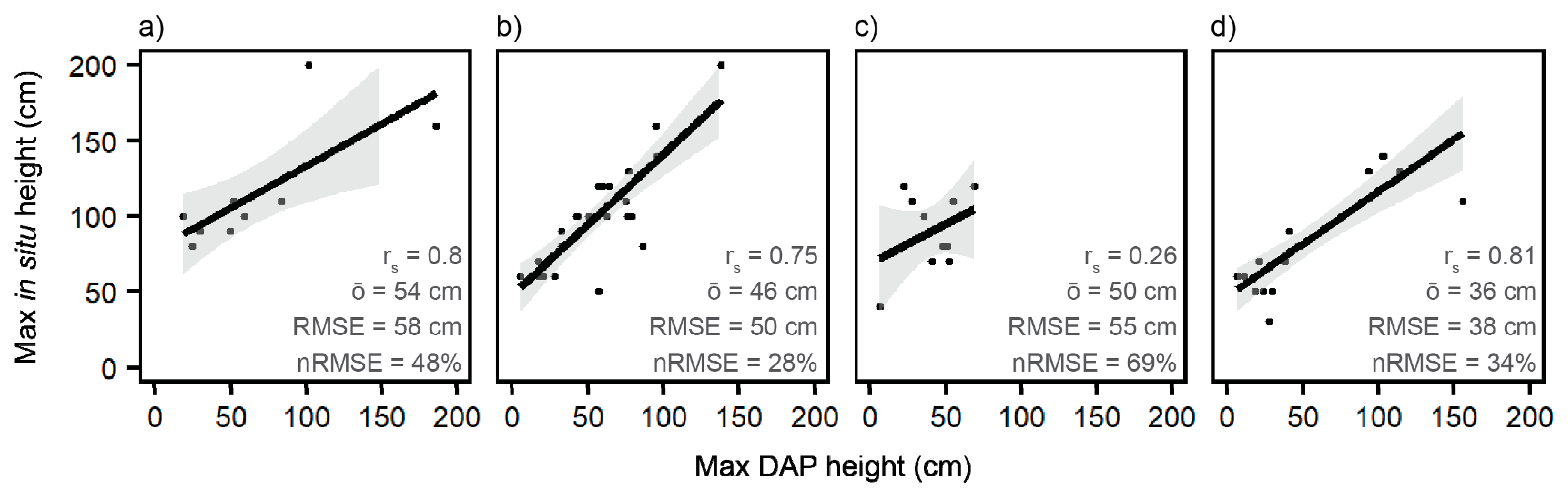
The relationship between maximum in situ and DAP height was investigated by life form (conifer, deciduous, graminoid, and perennial) using transect-based cells. Figure 3 shows strong correlations (rs > 0.75) for all lifeforms, except for graminoid species (rs = 0.26) with p-values < 0.05. However, DAP heights were consistently underestimated, expressed by large mean height offsets, ranging from 35.6 cm for perennials and 54.4 cm for conifers. According to the slope of the linear regression lines, height offsets of deciduous vegetation samples are consistent throughout all height strata, while offsets of samples representative of the other three life forms are greater for short vegetation (<75 cm) than tall vegetation. Offsets between DAP and in situ height were consistent across study sites ranging from an average offset of 44.1 cm for site B to 47.0 cm for site A.
3.2. Clustering Analysis
We extracted structure metrics, examined multicollinearity, and performed a clustering analysis including k-means++ pre-clustering and agglomerative hierarchal clustering. Table 5 shows cross-correlations of the five selected structure metrics. Correlations are typically much lower than rp = 0.8. Max and RI (rp = 0.80) and Max and %P25_200 (rp = 0.78) are the exception. Again, all p-values were < 0.05.
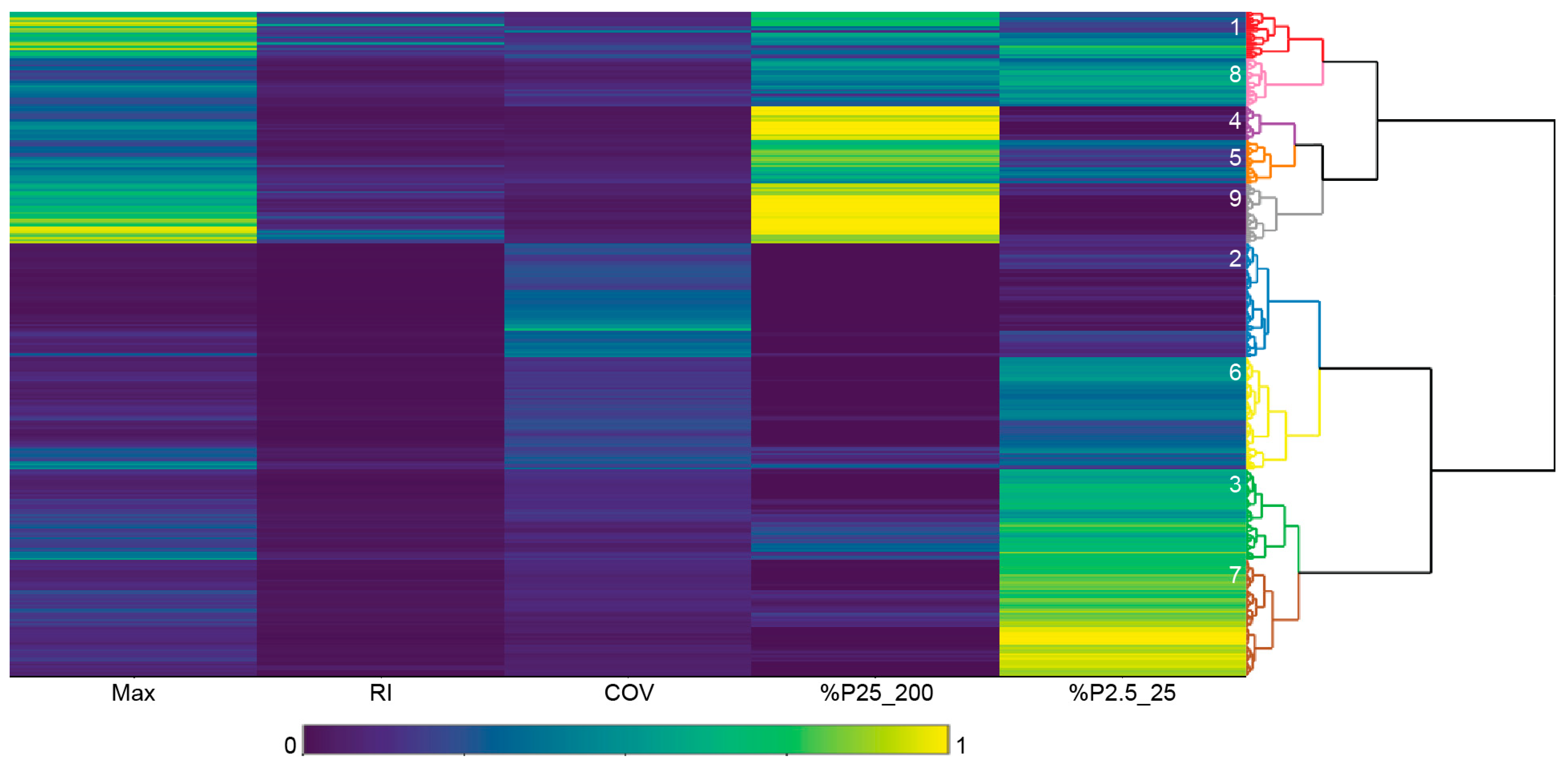
Figure 4 illustrates the optimal number of clusters (k) selected based on 325 pre-clusters was nine, which is where intra-cluster variation is maximized while a small number of clusters is maintained. Sharp increases of the gap statistic were found up to a k of seven. The dendrogram in Figure 5 shows the similarity between pre-clusters according to a distance matrix and agglomerative hierarchical clustering. The final clusters were color-coded based on the optimal k. The dendrogram consists of stacked branches that partition the pre-clusters into more homogeneous clusters. This means that clusters one and eight were more similar than clusters eight and four. The heatmap in Figure 5 shows the structure metrics for the pre-clusters, all scaled from zero to one. The metrics facilitated cluster characterization and interpretation, for example, cluster nine could be distinguished based on %P25_200 (close to one) and Max (between 0.6 and one). Note that metrics of a few clusters showed more similarity with distant clusters than with neighboring clusters, for example, clusters three with eight.
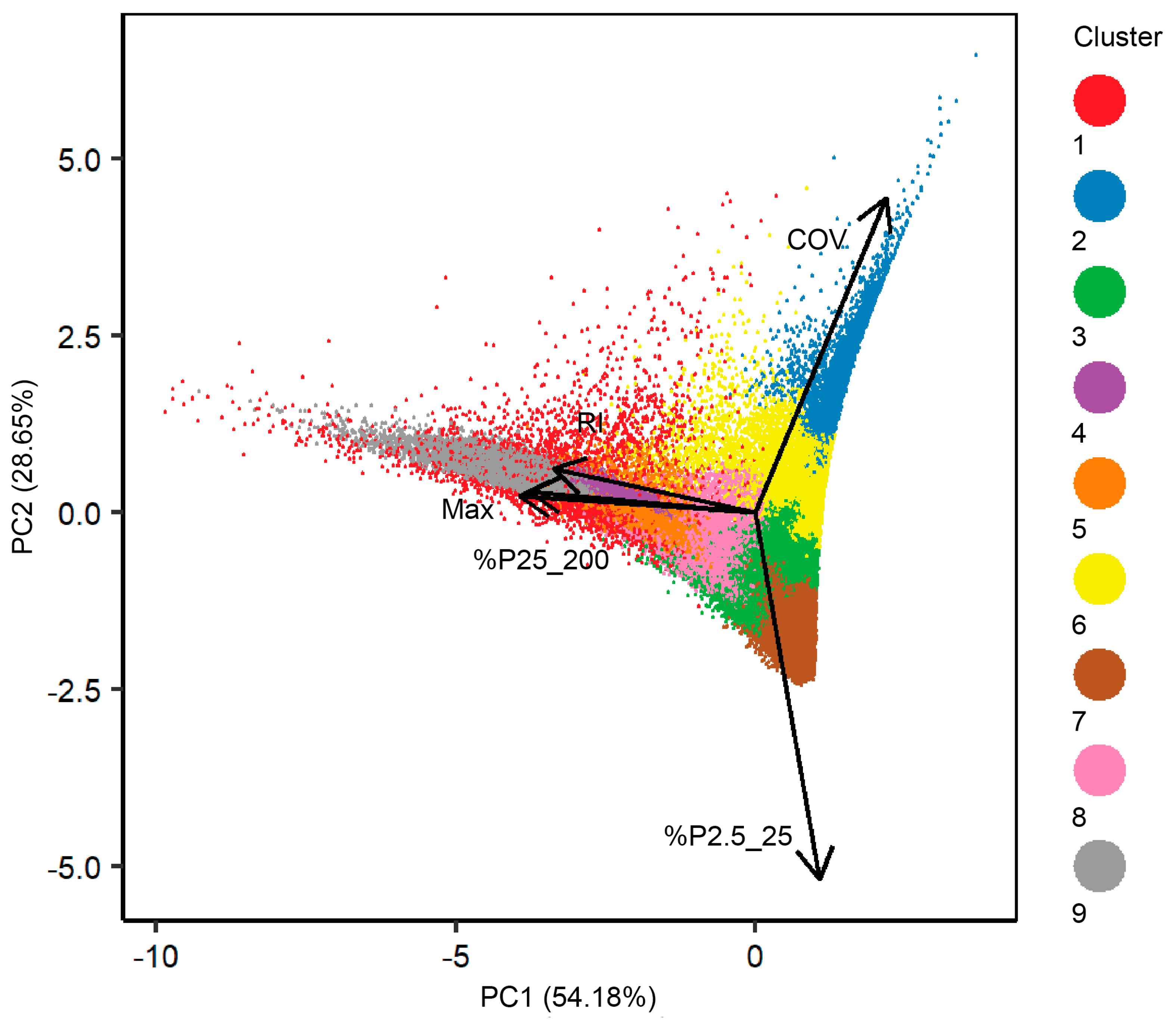
Principle components 1 and 2 described 54% and 28% of the total variance in the dataset (Figure 6). The direction of the vectors, or loadings, indicates how metrics drive the separability of the clusters. COV and %P2.5_25 were most influential in terms of discriminatory power among clusters and drove separability among clusters associated with relatively short-stature vegetation and homogenous canopy heights. The stronger correlated metrics, which included Max, RI, and %P25_200, drove separability of the clusters with larger vegetation and more heterogeneous structures. In more detail, COV drove the separability of cluster two and six, and %P2.5_25 drove the separability of cluster three, seven, and eight. Cluster three and eight, which show high overlap along the vector associated with %P2.5_25 in Figure 6, could be separated from each other based on Max, RI, and %P25_200.
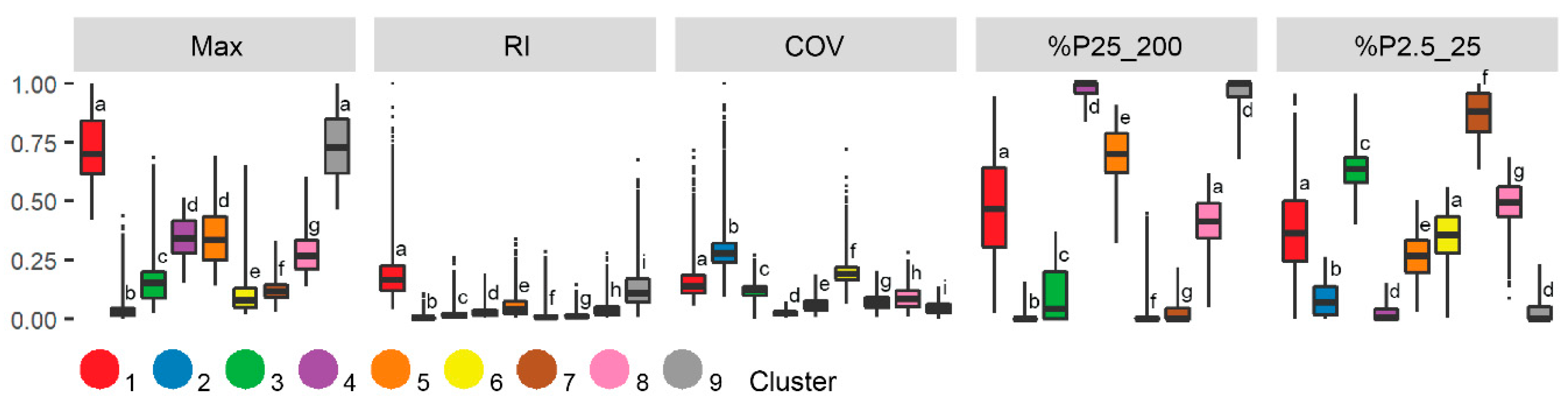
Figure 7 compares the structure metrics across nine clusters. Generally, three groupings of clusters can be discerned, principally based on maximum height. The first group consisting of cluster one and nine had a standardized height around 0.75 (~150 cm). The second group included cluster four and five approximately 0.37 (~80 cm) and the remaining clusters lower than 0.2 (~40 cm). The first group also showed relatively high RI values and was representative of relatively tall vegetation and complex canopy structures. The second group showed relatively high %P25_200 values and was characteristic of medium-tall vegetation and high canopy cover. In addition, RI and COV indicated a relatively smooth canopy for clusters in the second group. The third group was characterized by relatively low or no canopy cover, indicated by %P2.5_25 and %P25_200, and a smooth to extremely smooth canopy surface, indicated by RI and COV.
Within the three groups, we found subtle differences across metrics related to canopy cover and height variability. In the first and second groups, one of the clusters was characteristic of a more closed and flatter canopy, clusters nine and four, respectively, while their counterparts had a more open canopy. Differences between clusters in the third group were small, although the clusters were still significantly different (p < 0.01). We found clusters characterized by the absence of vegetation structure, including cluster two and six, as well as clusters with very short vegetation (three, seven, and eight). Clusters in the third group can be characterized in more detail with the height and cover between 2.5 and 25 cm greater for cluster six compared to two, likely indicating some presence of very low stature vegetation. Clusters three, seven, and eight all had high total canopy cover, but cluster seven stood out as %P2.5_25 was close to 1, which is representative of dense, very short vegetation.
3.3. Final Structure Classes
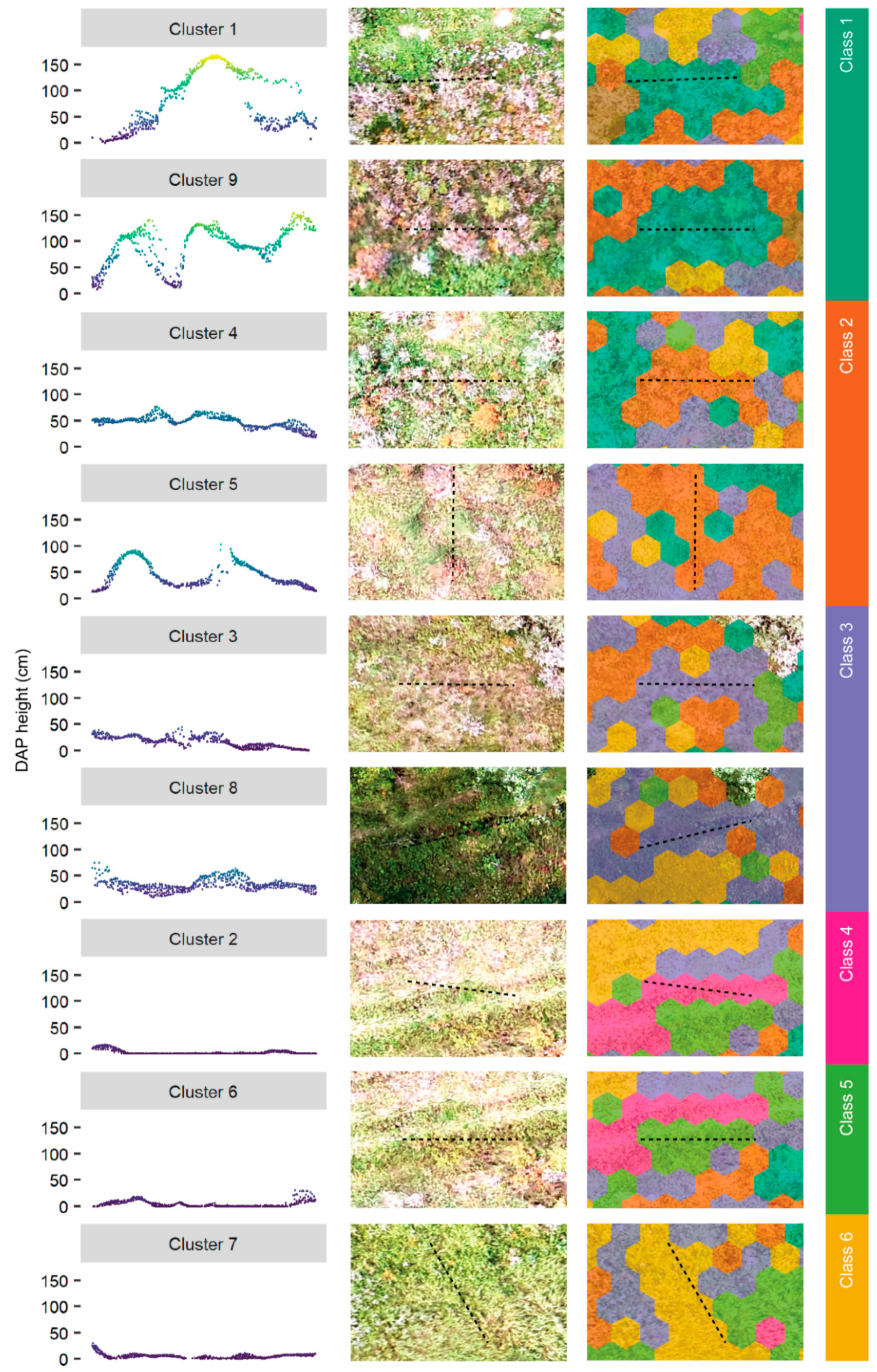
We merged the clusters into final classes based on the structure metrics, point-cloud visualizations, and field observations. The final classes, including structural descriptions and indicative life forms, are summarized in Table 6, and representative point clouds are illustrated in Figure 8 using cross-sections. Relatively tall and complex vegetation was represented by classes one and two. Field observations indicated the presence of woody vegetation, predominantly willow (Salix spp.) shrubs, was characteristic of class one. Single occurrences of aspen poplar and lodgepole pine were also found. Class two was characterized by tall (>50 cm) graminoids and perennials including yellow sweet clover and white clover. A few noxious weed species were recorded in the in situ transects overlapping with class two. The difference in canopy height heterogeneity between underlying clusters, described in the previous paragraph, was related to the inclusion of more exposed soil and short vegetation, e.g., graminoids. Figure 8 illustrates that clusters one and five were found on boundaries of vegetation patches or include single isolated plants.
Classes three to six were characteristic of short-stature vegetation with homogenous canopy height and vegetation structure absent. Class three, which is based on two merged clusters, was characterized by the presence of graminoid species and short perennials such as white clover. The cross-sections in Figure 8 illustrate strong similarity among classes four, five, and six, all of which characterized the absence of vegetation structure, however, differences exist. Class four is absent of vegetation structures and characterized by exposed soil, mosses, and short grass. Class five includes mosses, short grasses, and small seedlings (approximately 30 to 40 cm). Class six is representative of short graminoids and perennials, that sometimes grew together with small seedlings, including aspen, black spruce, and willow.
3.4. Land Cover and Spatial Arrangement
Figure 9a shows the proportions of structural classes by site. Total cover by relatively large and complex structures, presumably woody vegetation, was highest at site A (Lower Boreal Highlands) with 35.2% followed by site C (Upper Foothills) and B (Lower Boreal Highlands) with 27.6% and 13.9%, respectively. Site A was mostly covered by young woody vegetation shorter than 1.5 m (class one; 22%) followed by short as well as mid-tall vegetation structures representing graminoids and perennials (class two and three; 37.1%). In contrast, site C had a high cover of developed woody vegetation (class seven; 19.6%) and absent or near-absent vegetation structures (class four and five; 40.5%) but relatively low cover by classes representative of short graminoids and perennials (classes two, three, and six; 31.8%) and young woody vegetation (class two; 8%). Cover percentages found at Site B were similar to site C except for the cover by short dense vegetation structures (class six; 20.1%) being more than twice as high as the developed woody vegetation cover (class seven; 7.5%).
Patch size distributions of the structural classes are shown in Figure 9b and indicate that across all sites the largest mean patch size occurred for class seven, ranging from 10.6 m2 for site A to 26.3 m2 for site C. At site A, the second largest mean patch size was for class one, representing young regenerating woody vegetation. At sites B and C, there were also a number of areas of class four with vegetation structures absent with mean patch sizes of 8.3 and 13.7 m2, respectively. In addition, relatively large patches with very short vegetation structures and homogenous canopy heights, representative of class six, were found at site B. The mean patch size of class six at this site was 6.1 m2. The remaining classes at all sites had mean patch sizes ranging from 2.4 to 4.3 m2.
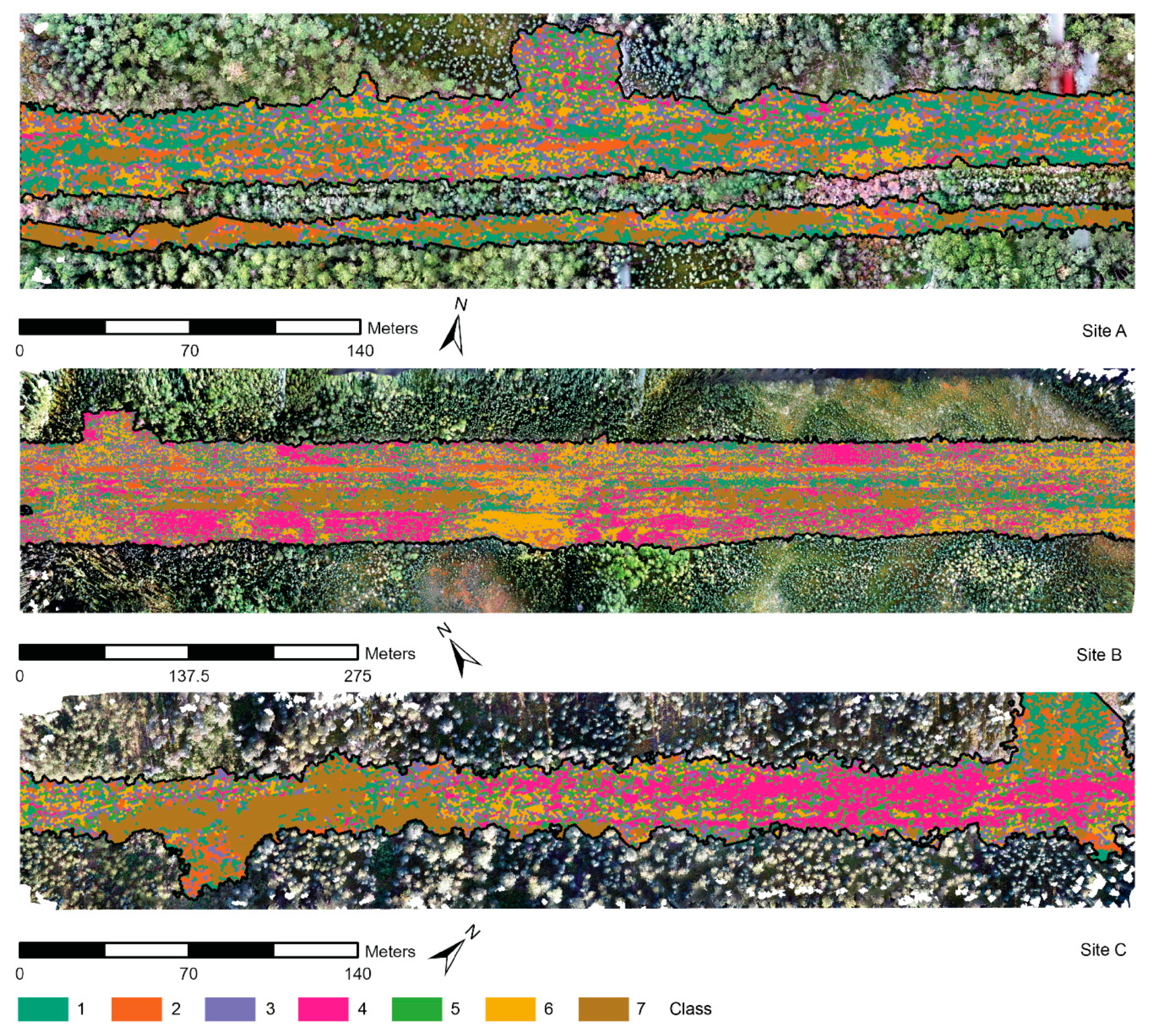
Figure 10 shows maps of the structural vegetation classes across the three sites based on the classified 1 m2 hexagons. Multiple adjacent ROWs, including an approximately 30-m-wide ROW of a pipeline constructed in 2009 and a 10-m-wide ROW, were observed at site A with varying compositions of vegetation structure. The narrow ROW was predominantly covered by large patches with tall and complex vegetation structures representative of classes one and seven, with an anticipated trajectory towards a mature forest. A small section with mid-to-tall vegetation representative of class two, presumably tall graminoids and perennials, was found in the east section. A complex mosaic of structure classes was found on the wide ROW. Relatively large patches with regenerating woody vegetation representative of class one were observed that connected both sides of the ROW at three sections. Patches representative of very short but dense vegetation structures, characterized by class six, connected both sides of the ROW at the east section. Long, narrow continuous patches representative of class two, characterizing tall graminoids and perennials, were found in the middle of the wide ROW.
Site B included an approximately 75 m wide ROW on which multiple parallel sections with distinctive vegetation structures were found. The southwestern half of the ROW, which included a power line, had large amounts of class four (vegetation structure absent) and six (very short but dense vegetation structures). This half was largely separated by vegetation representative of class seven. The northeastern section, which includes three pipelines, included long, narrow stretches of young regenerating woody vegetation representative of class one. Stretches of tall perennials and graminoids representative of class two were also observed. Lastly, a few relatively large patches of class four were found adjacent to the forest edge.
At cite C, which included an approximately 26-m-wide ROW of a single pipeline, two major areas were observed with a high cover of predominantly a single structure class. A large continuous area with vegetation representative of class seven was found in the western section (left), while vegetation characteristic of class four (structures absent) was predominantly found in the eastern section (right).
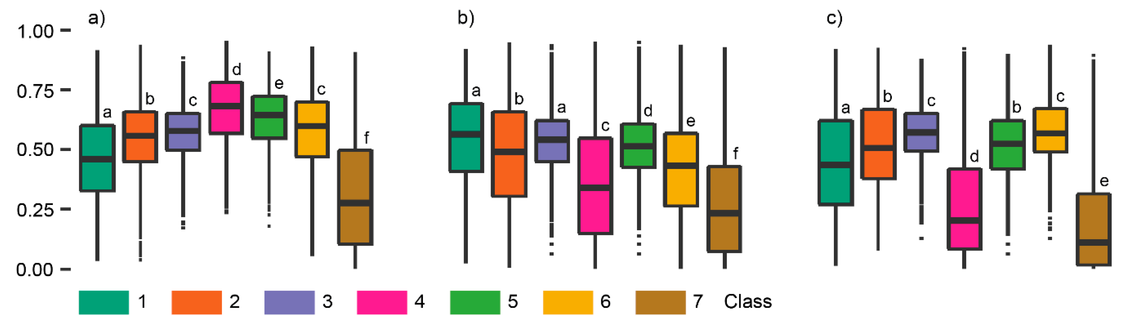
Measures of local spatial association between structure classes by site, using entropy-based local spatial association (ELSA) scores ranging from zero to one are shown in Figure 11. At site A, relatively low ELSA scores were found for class one and seven indicating both classes occur generally in patches, having a median of 0.47 and 0.25, respectively. Class four, which is closely followed by class five, had the highest scores, indicating hexagons representative of absent or almost-absent vegetation structures were generally randomly distributed at site A. Contrarily, at sites B and C, class four showed relatively low ELSA scores of 0.37 and 0.2, respectively, indicating hexagons with vegetation structures absent typically occurring in patches. At site B, young woody vegetation (class one) and short graminoids and perennials (class three) show the same level of random distribution, both having a median ELSA score of approximately 0.55. At site C, classes three and six had the highest scores with medians around 0.5.
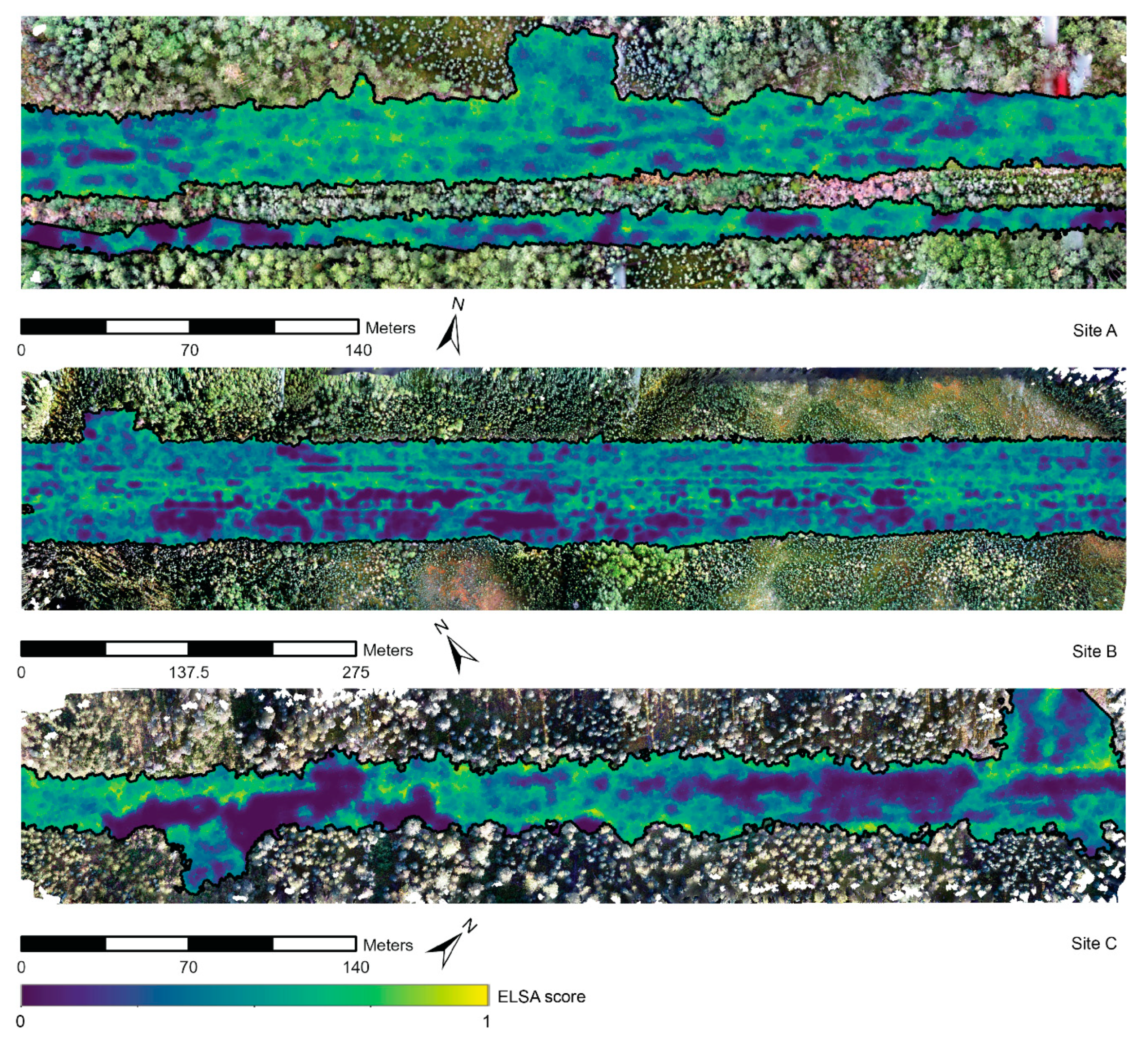
Figure 12 shows maps of the three study sites indicating the level of local spatial association based on all classified hexagons. At site A, relatively low ELSA scores were found at multiple locations on the narrow ROW. ELSA scores were relatively high in the ROW’s east section indicating a more random class distribution of class two. The wide ROW showed generally high ELSA scores but included some sections with high patchiness. In the west section (left), patches were representative of regenerating or more developed woody vegetation. In the east section (right), patches were found of class six, representative of very short but dense vegetation structures, that largely formed a connection between the ROW’s boundaries.
At site B, multiple parallel stretches, as well as large sections adjacent to the ROW’s boundaries, had low ELSA scores. At the southwestern half of the ROW (bottom), areas of bare ground surface were highly patchy, becoming more random towards the eastern (right) locations. Lastly, at site C, two extensive sections with high patchiness were present in the southwest (left) and northeast (right).
4. Discussion
The past five years have seen considerable progress on the application of DAP for characterizing short vegetation structures for monitoring, however, research has principally been focused on DAP height measurement or mapping of structures in sparsely vegetated landscapes such as savannas [25,26,29]. This study focused on areas of ongoing anthropogenic disturbance in temperate coniferous and boreal forest ecoregions which are generally densely vegetated and include heterogeneous mosaics of early successional vegetation types. The incorporation of metrics derived over a regularized surface, describing vegetation height, cover, variability, and surface complexity, allowed a more detailed characterization of vegetation patterns than studies that simply utilize the canopy height model such as [25].
Concurrently, innovations in drone design are resulting in systems with longer flight range and speed, improved autopilot and safety features, and greater maximum payloads [69,70]. Furthermore, drones are becoming more user-friendly due to plug-and-play sensor systems, improved smartphone-operated mission planning software, and in cloud processing [69]. New drone-specific aviation legislation and streamlined permit systems have been implemented by Canadian, American, and, as of 2021, European aviation safety agencies, making it easier and safer for organizations to start deploying drones [71,72].
In our study, DAP heights were underestimated and show reduced height variability, which is in line with findings of [29]. This can be explained by height error introduced during data collection, DAP processing, or ground filtering, being close to short-stature vegetation height. Observed RMSE values ranged from 38 to 58 cm for various life forms, while [29] found values in the range of 20 to 46 cm for two height strata (0 to 0.5 m and 0.51 to 2.0 m) at comparable sites with respect to forest type, disturbance type, and successional stage. Different flight parameters could have caused such a discrepancy. An investigation by [73] found that small image pitch angle, high solar elevation, and low flight altitudes ideally between 25 and 50 m (while retaining high image overlap) improved structure measurements of tree crops. We acknowledge that high flight altitudes (90 to 180 m), chosen to comply with visual line-of-sight requirements and limit data acquisition time, may have reduced data quality in our study. In addition, image pitch angles from the DJI Phantom 4 acquired imagery were highly variable. High bidirectional reflectance was observed above exposed soil at sites A and B and heavy shadowing was found at site C. Our study suggests that errors can partially be explained by vegetation characteristics. The large height offsets found for conifers suggest that DAP has difficulties resolving seedlings that ideally stand out more clearly and form an unambiguous structure class. This could be caused by a combination of flight altitude, illumination conditions, and, as a result, issues with the identification of treetops during image matching. Automated ground filtering can become problematic in densely vegetated areas [30,74] which could explain the large normalized RMSE found for graminoids. Novel flight protocols including oblique imagery such as those developed by [25,31] can produce very detailed reconstructions of graminoid and shrub canopies as well as terrain, however, this will require multiple consecutive flights. We recommend further investigation of optimal flight parameters for short-stature vegetation, which should also consider battery performance and flight time.
Despite these technological issues, direct measurements of height and canopy attributes were accurate and allowed us to distinguish three broad groupings of structure associated with young woody vegetation, large perennials, and graminoids as well as remaining short-stature vegetation. Subtle differences in metrics describing height variability and canopy cover allow for the classification of the shortest vegetation structures representative of meadow grasses, seedlings, short shrubby, and herbaceous perennials. Previously, [61] demonstrated that such metrics enabled the characterization of forest stand structure from LiDAR. Early successional vegetation shows much less layering along the vertical dimension but higher structural variation along the horizontal dimension compared to mature forests, which may explain the success of comparable metrics for the classification of short vegetation structures from DAP. Note that DAP typically has a higher spatial resolution in comparison to conventionally flown LiDAR point clouds but is limited to characterization of the top canopy.
Hexagon-based clustering analysis using ELSA provided maps of vegetation structures at relevant spatial and thematic scales for ecologists and restoration professionals, requiring limited field sampling for validation and interpretation purposes. Traditional studies based on field sampling are constrained by time, costs, and resources, which may result in arbitrarily chosen scales of observation, not well-matched with scales of ecological processes or environmental variables [18,20]. Such risks are now partially averted, as underlying environmental variables and processes can be worked out after data acquisition based on shape, location, and patterns of patches of particular structure classes.
Some unambiguous restoration objectives are analogous to vegetation structure [11]. Such objectives, including soil stabilization and undesirable species control, can be monitored using combined measures of structural cover, patch size, and spatial arrangement. Areas of potential erosion could be identified based on cover without structures in combination with associated levels of patchiness as illustrated by Figure 9 and Figure 11. Mapped shapes and patterns can support restoration professionals by describing and identifying underlying factors such as existing erosion, terrain wetness, seedbank issues, or soil conditions. In addition, where erosion control includes willow or shrub staking [42], vegetation establishment can potentially be tracked using the developed tools. One of the shortcomings of our approach is that species composition is hard to determine, which is necessary for assessing the presence of invasive species. Alternatively, restoration professionals may find that specific structural vegetation classes are more likely to represent undesirable species or, if showing high patchiness, limit successional development towards a treed environment.
Future studies should investigate the potential for the application of off-the-shelf multispectral and hyperspectral drone-based sensors, in combination with spectral vegetation indices that capture unique characteristics of plant reflectance, for improving effective discrimination between plant communities. Where a structural or spectral dataset alone may not be able to resolve the boundaries of a plant community, a combination of the two may improve discrimination as demonstrated by [75]. In addition, it is important to investigate the consistency of the derived information under varying flight parameters and develop novel flight protocols considering simplicity, cost-effectiveness, and quality of derived information. Considering that there is a growing push for the restoring and monitoring of sites impacted by resource extraction, as well as interest in monitoring of present-day reference sites within the ecological restoration community [76], we suggest that drones will play an increasingly important role in forest restoration projects in the future.
5. Conclusions
Our approach demonstrates how drone-based DAP can be used to characterize short-stature vegetation structures on sites displaying a complex mosaic of vegetation types typical for temperate and boreal coniferous forests in Alberta, Canada. Extraction of classes representative of mid-to-tall vegetation structures, such as young woody vegetation, tall graminoids, and perennials, is relatively straightforward based on metrics describing canopy height and surface complexity, while more carefully selected metrics describing canopy cover and height variability are necessary to obtain classes of most short-stature vegetation structures. The spatial arrangement of mapped structures can improve our understanding of vegetation patterns, which could help to describe the driving environmental variables and processes of ecological succession within the landscape. In return, this could support the evaluation in relation to restoration objectives, as well as prioritization of mitigation measures and future monitoring. We anticipate that optimized flight protocols, optimal weather conditions, and enhanced sensors can further improve the capability of DAP to characterize early regenerative vegetation structures.
Author Contributions
Conceptualization, R.J.G.N., N.C.C., and C.W.; pre-processing, R.J.G.N.; formal analysis, R.J.G.N.; investigation, R.J.G.N.; methodology, R.J.G.N.; resources, R.J.G.N.; supervision, N.C.C. and C.W.; visualization, R.J.G.N.; writing—original draft, R.J.G.N.; writing—review and editing, R.J.G.N., N.C.C., C.W., and D.T. All authors have read and agreed to the published version of the manuscript.
Funding
This research was funded by TC Energy and Natural Sciences and Engineering Research Council of Canada (NSERC) grant CRDPJ 537625–18.
Acknowledgments
We thank the drone pilots from Midwest Surveys for their dedication to data acquisition and all staff from TC Energy that initiated and supported our research. We would like to thank our field crew from the Integrated Remote Sensing Studio at UBC Forestry and our environmental officer from TC Energy that provided us with the much-needed technical and species identification skills. We would like to thank Cindy Prescott of UBC’s Department of Forest and Conservation Sciences for editing the final manuscript. We thank all anonymous reviewers and journal editorial staff for their efforts in improving the quality of this manuscript.
Conflicts of Interest
The authors declare no conflict of interest.
References
- Lambin, E.F.; Meyfroidt, P. Global land use change, economic globalization, and the looming land scarcity. Proc. Natl. Acad. Sci. USA 2011, 108, 3465–3472. [Google Scholar] [CrossRef] [PubMed] [Green Version]
- British Petroleum. Energy Outlook 2020 Edition Explores the Forces Shaping the Global Energy Transition out to 2050 and the Surrounding That Transition; British Petroleum: London, UK, 2020. [Google Scholar]
- Food and Agriculture Organization of the United Nations. The State of the World’s Forests; Food and Agriculture Organization of the United Nations: Rome, Italy, 2020. [Google Scholar]
- Convention on Biological Diversity. Invasive Alien Species: A Threat to Biodiversity; Convention on Biological Diversity: Quebec, QC, Canada, 2009. [Google Scholar]
- Dabros, A.; Pyper, M.; Castilla, G. Seismic lines in the boreal and arctic ecosystems of North America: Environmental impacts, challenges, and opportunities. Environ. Rev. 2018, 26, 214–229. [Google Scholar] [CrossRef] [Green Version]
- Aerts, R.; Honnay, O. Forest restoration, biodiversity and ecosystem functioning. BMC Ecol. 2011, 11, 1–21. [Google Scholar] [CrossRef] [Green Version]
- Ciccarese, L.; Mattsson, A.; Pettenella, D. Ecosystem services from forest restoration: Thinking ahead. New For. 2012, 43, 543–560. [Google Scholar] [CrossRef]
- McClung, M.R.; Moran, M.D. Understanding and mitigating impacts of unconventional oil and gas development on land-use and ecosystem services in the U.S. Curr. Opin. Environ. Sci. Heal. 2018, 3, 19–26. [Google Scholar] [CrossRef]
- Bendor, T.; Lester, T.W.; Livengood, A.; Davis, A.; Yonavjak, L. Estimating the size and impact of the ecological restoration economy. PLoS ONE 2015, 10, 1–15. [Google Scholar] [CrossRef]
- National Energy Board. Environmental Protection Plan Guidelines; National Energy Board: Calgary, AB, Canada, 2011. [Google Scholar]
- Prach, K.; Durigan, G.; Fennessy, S.; Overbeck, G.E.; Torezan, J.M.; Murphy, S.D. A primer on choosing goals and indicators to evaluate ecological restoration success. Restor. Ecol. 2019, 27, 917–923. [Google Scholar] [CrossRef]
- Stanturf, J.A.; Palik, B.J.; Dumroese, R.K. Contemporary forest restoration: A review emphasizing function. For. Ecol. Manage. 2014, 331, 292–323. [Google Scholar] [CrossRef]
- Thorpe, A.S.; Stanley, A.G. Determining appropriate goals for restoration of imperilled communities and species. J. Appl. Ecol. 2011, 48, 275–279. [Google Scholar] [CrossRef]
- Murphy, S.D. Restoration Ecology’s Silver Jubilee: Meeting the challenges and forging opportunities. Restor. Ecol. 2018, 26, 3–4. [Google Scholar] [CrossRef]
- Dale, V.H.; Beyeler, S.C. Remote sensing of vegetation 3-D structure for biodiversity andhabitat: Review and implications for lidar and radar spacebornemissions. Ecol. Indic. 2001, 1, 3–10. [Google Scholar] [CrossRef] [Green Version]
- Gibbons, P.; Freudenberger, D. An overview of methods used to assess vegetation condition at the scale of the site. Ecol. Manag. Restor. 2006, 7, 10–17. [Google Scholar] [CrossRef]
- D’Urban Jackson, T.; Williams, G.J.; Walker-Springett, G.; Davies, A.J. Three-dimensional digital mapping of ecosystems: A new era in spatial ecology. Proc. R. Soc. B Biol. Sci. 2020, 287, 1–10. [Google Scholar] [CrossRef] [Green Version]
- Levin, S.A. The problem of pattern and scale in ecology. Ecology 1992, 73, 1943–1967. [Google Scholar] [CrossRef]
- Anderson, K.; Gaston, K.J. Lightweight unmanned aerial vehicles will revolutionize spatial ecology. Front. Ecol. Environ. 2013, 11, 138–146. [Google Scholar] [CrossRef] [Green Version]
- Wheatley, M.; Johnson, C. Factors limiting our understanding of ecological scale. Ecol. Complex. 2009, 6, 150–159. [Google Scholar] [CrossRef]
- Bergen, K.M.; Goetz, S.J.; Dubayah, R.O.; Henebry, G.M.; Hunsaker, C.T.; Imhoff, M.L.; Nelson, R.F.; Parker, G.G.; Radeloff, V.C. Remote sensing of vegetation 3-D structure for biodiversity and habitat: Review and implications for lidar and radar spaceborne missions. J. Geophys. Res. Biogeosciences 2009, 114, 1–10. [Google Scholar] [CrossRef] [Green Version]
- Wulder, M.A.; Bater, C.W.; Coops, N.C.; Hilker, T.; White, J.C. The role of LiDAR in sustainable forest management. For. Chron. 2008, 84, 807–826. [Google Scholar] [CrossRef] [Green Version]
- Forsmoo, J.; Anderson, K.; Macleod, C.J.A.; Wilkinson, M.E.; DeBell, L.; Brazier, R.E. Structure from motion photogrammetry in ecology: Does the choice of software matter? Ecol. Evol. 2019, 9, 12964–12979. [Google Scholar] [CrossRef]
- Colomina, I.; Molina, P. Unmanned aerial systems for photogrammetry and remote sensing: A review. ISPRS J. Photogramm. Remote. Sens. 2014, 92, 79–97. [Google Scholar] [CrossRef] [Green Version]
- Cunliffe, A.M.; Brazier, R.E.; Anderson, K. Ultra-fine grain landscape-scale quantification of dryland vegetation structure with drone-acquired structure-from-motion photogrammetry. Remote Sens. Environ. 2016, 183, 129–143. [Google Scholar] [CrossRef] [Green Version]
- van Iersel, W.; Straatsma, M.; Addink, E.; Middelkoop, H. Monitoring height and greenness of non-woody floodplain vegetation with UAV time series. ISPRS J. Photogramm. Remote Sens. 2018, 141, 112–123. [Google Scholar] [CrossRef]
- Quirós Vargas, J.J.; Zhang, C.; Smitchger, J.A.; McGee, R.J.; Sankaran, S. Phenotyping of Plant Biomass and Performance Traits Using Remote Sensing Techniques in Pea (Pisum sativum, L.). Sensors 2019, 19, 2031. [Google Scholar] [CrossRef] [PubMed] [Green Version]
- White, J.C.; Wulder, M.A.; Vastaranta, M.; Coops, N.C.; Pitt, D.; Woods, M. The utility of image-based point clouds for forest inventory: A comparison with airborne laser scanning. Forests 2013, 4, 518–536. [Google Scholar] [CrossRef] [Green Version]
- Chen, S.; McDermid, G.J.; Castilla, G.; Linke, J. Measuring vegetation height in linear disturbances in the boreal forest with UAV photogrammetry. Remote Sens. 2017, 9, 1257. [Google Scholar] [CrossRef] [Green Version]
- Zahawi, R.A.; Dandois, J.P.; Holl, K.D.; Nadwodny, D.; Reid, J.L.; Ellis, E.C. Using lightweight unmanned aerial vehicles to monitor tropical forest recovery. Biol. Conserv. 2015, 186, 287–295. [Google Scholar] [CrossRef] [Green Version]
- James, M.R.; Robson, S. Mitigating systematic error in topographic models derived from UAV and ground-based image networks. Earth Surf. Process. Landf. 2014, 39, 1413–1420. [Google Scholar] [CrossRef] [Green Version]
- Government of Canada. Natural Gas Facts. Available online: https://www.nrcan.gc.ca/science-data/data-analysis/energy-data-analysis/energy-facts/natural-gas-facts/20067#L1 (accessed on 1 June 2020).
- Canada Energy Regulator. Canada’s Energy Future 2020; Canada Energy Regulator: Calgary, AB, Canada, 2020. [Google Scholar]
- Northrup, J.M.; Wittemyer, G. Characterising the impacts of emerging energy development on wildlife, with an eye towards mitigation. Ecol. Lett. 2013, 16, 112–125. [Google Scholar] [CrossRef]
- Dabros, A.; James Hammond, H.E.; Pinzon, J.; Pinno, B.; Langor, D. Edge influence of low-impact seismic lines for oil exploration on upland forest vegetation in northern Alberta (Canada). For. Ecol. Manage. 2017, 400, 278–288. [Google Scholar] [CrossRef]
- Government of Canada. Considerations in Developing Oil and Gas Industry Best Practices in the North; Government of Canada: Whitehorse, YT, Canada, 2009.
- Canadian Energy Regulator. Lifecycle Approach. Available online: https://www.cer-rec.gc.ca/en/safety-environment/environment/index.html (accessed on 1 June 2020).
- TC Energy. Year Three Caribou Monitoring Report—NWML, LKXO and Chinchaga Project; TC Energy: Calgary, AB, Canada, 2020. [Google Scholar]
- Alberta Energy Regulator Data and Reports: Pipelines and Other Infrastructure. Available online: https://www.aer.ca/providing-information/data-and-reports/statistical-reports/st98/pipelines-and-other-infrastructure (accessed on 1 June 2020).
- Desserud, P.; Gates, C.C.; Adams, B.; Revel, R.D. Restoration of foothills rough fescue grassland following pipeline disturbance in Southwestern Alberta. J. Environ. Manage. 2010, 91, 2763–2770. [Google Scholar] [CrossRef]
- Caners, R.T.; Lieffers, V.J. Divergent pathways of successional recovery for in situ oil sands exploration drilling pads on wooded moderate-rich fens in alberta, Canada. Restor. Ecol. 2014, 22, 657–667. [Google Scholar] [CrossRef]
- Barker, J. Minimum disturbance pipeline construction in boreal forests to reduce restoration challenges. In Proceedings of the SER-WC: Restoration for Resilience—Ecological Restoration in the 21st Century, Burnaby, BC, Canada, 14–16 February 2018; pp. 1–29. [Google Scholar]
- Government of Alberta. Provincial Woodland Caribou Range Plan: Alberta’s Approach to Achieve Caribou Recovery (Draft); Government of Alberta: Edmonton, AB, Canada, 2017.
- TC Energy. Restoration Plan for the Chinchaga Lateral Loop No. 3 (Chinchaga Section); TC Energy: Calgary, AB, Canada, 2014. [Google Scholar]
- Eyre, M.; Kerkhof, S.; Pfeiffer, Z.; Titman, S. Cumulative Effects, woodland caribou and NEB regulated pipelines—A regultory perspective. In Proceedings of the 11th Symposium on Environmental Concerns in RoW Management, Halifax, NS, Canada, 20–23 September 2015; pp. 267–279. [Google Scholar]
- Government of Alberta. Weed Control Act. Alberta Regulation AR 171/2001; Government of Alberta: Edmonton, AB, Canada, 2010.
- TC Energy. Third Year Post-Construction Monitoring Report for the NOVA Gas Transmission LTD. Musreau Cutbank Expension; TC Energy: Calgary, AB, Canada, 2019. [Google Scholar]
- Natural Regions Committee. Natural Regions and Subregions of Alberta. Compiled by D.J. Downing and W.W. Pettapiece; Natural Regions Committee: Edmonton, AB, Canada, 2006. [Google Scholar]
- Alberta Parks. Natural Regions and Subregions of Alberta: A Framework for Alberta’s Parks; Alberta Parks: Edmonton, AB, Canada, 2015. [Google Scholar]
- Willkomm, M.; Bolten, A.; Bareth, G. Non-destructive monitoring of rice by hyperspectral in-field spectrometry and UAV-based remote sensing: Case study of field-grown rice in North Rhine-Westphalia, Germany. Int. Arch. Photogramm. Remote. Sens. Spat. Inf. Sci. ISPRS Arch. 2016, XLI-B1, 1071–1077. [Google Scholar] [CrossRef] [Green Version]
- Province of Alberta. Weed Control Act Statutes of Alberta Chapter W-5.1; Province of Alberta: Edmonton, AB, Canada, 2008; pp. 1–14. [Google Scholar]
- Agisoft LLC. Agisoft Metashape Professional v1.6.3; Agisoft LCC: Saint Petersburg, Russia, 2020. [Google Scholar]
- Chiabrando, F.; Donadio, E.; Rinaudo, F. SfM for orthophoto generation: A winning approach for cultural heritage knowledge. Int. Arch. Photogramm. Remote. Sens. Spat. Inf. Sci. ISPRS Arch. 2015, 40, 91–98. [Google Scholar] [CrossRef] [Green Version]
- Murtiyoso, A.; Grussenmeyer, P.; Börlin, N.; Vandermeerschen, J.; Freville, T. Open source and independent methods for bundle adjustment assessment in close-range UAV photogrammetry. Drones 2018, 2, 3. [Google Scholar] [CrossRef] [Green Version]
- Granshaw, S.I. Bundle Adjustment Methods in Engineering Photogrammetry. Photogramm. Rec. 1980, 10, 181–207. [Google Scholar] [CrossRef]
- Isenburg, M. LAStools-Efficient Tools for LiDAR Processing. Available online: https://rapidlasso.com/lastools/ (accessed on 10 January 2020).
- Anders, N.; Valente, J.; Masselink, R.; Keesstra, S. Comparing Filtering Techniques for Removing Vegetation from UAV-Based Photogrammetric Point Clouds. Drones 2019, 3, 61. [Google Scholar] [CrossRef] [Green Version]
- Goodbody, T.R.H.; Coops, N.C.; Tompalski, P.; Crawford, P.; Day, K.J. Updating residual stem volume estimates using ALS- and UAV-acquired stereo-photogrammetric point clouds. Int. J. Remote Sens. 2016, 38, 2938–2953. [Google Scholar] [CrossRef]
- White, J.C.; Stepper, C.; Tompalski, P.; Coops, N.C.; Wulder, M.A. Comparing ALS and image-based point cloud metrics and modelled forest inventory attributes in a complex coastal forest environment. Forests 2015, 6, 3704–3732. [Google Scholar] [CrossRef]
- Jenness, J.S. Calculating landscape surface area from digital elevation models. Wildl. Soc. Bull. 2004, 32, 829–839. [Google Scholar] [CrossRef]
- Guo, X.; Coops, N.C.; Tompalski, P.; Nielsen, S.E.; Bater, C.W.; John Stadt, J. Regional mapping of vegetation structure for biodiversity monitoring using airborne lidar data. Ecol. Inform. 2017, 38, 50–61. [Google Scholar] [CrossRef]
- Wold, S.; Esbensen, K.; Geladi, P. Principal Component Analysis. Chemom. Intell. Lab. Syst. 1987, 2, 37–52. [Google Scholar] [CrossRef]
- Chiu, T.; Fang, D.P.; Chen, J.; Wang, Y.; Jeris, C. A robust and scalable clustering algorithm for mixed type attributes in large database environment. In Proceedings of the seventh ACM SIGKDD international conference on Knowledge discovery and data mining, San Francisco, CA, USA, 26–29 August 2001; pp. 263–268. [Google Scholar]
- Tamura, Y.; Obara, N.; Miyamoto, S. A method of two-stage clustering with constraints using agglomerative hierarchical algorithm and one-pass k-means++. Adv. Intell. Syst. Comput. 2014, 2, 9–19. [Google Scholar]
- Ward, J.H. Hierarchical Grouping to Optimize an Objective Function Author. J. Am. Stat. Assoc. 1963, 58, 236–244. [Google Scholar] [CrossRef]
- Dunn, O.J. Multiple Comparisons Using Rank Sums. Technometrics 1964, 6, 241–252. [Google Scholar] [CrossRef]
- Kruskal, W.H.; Wallis, W.A. Use of Ranks in One-Criterion Variance Analysis. J. Am. Stat. Assoc. 1952, 47, 583–621. [Google Scholar] [CrossRef]
- Naimi, B.; Hamm, N.A.S.; Groen, T.A.; Skidmore, A.K.; Toxopeus, A.G.; Alibakhshi, S. ELSA: Entropy-based local indicator of spatial association. Spat. Stat. 2019, 29, 66–88. [Google Scholar] [CrossRef]
- Crutsinger, G.M.; Short, J.; Sollenberger, R. The future of UAVs in ecology: An insider perspective from the Silicon Valley drone industry. J. Unmanned Veh. Syst. 2016, 4, 161–168. [Google Scholar] [CrossRef] [Green Version]
- Pádua, L.; Vanko, J.; Hruška, J.; Adão, T.; Sousa, J.J.; Peres, E.; Morais, R. UAS, sensors, and data processing in agroforestry: A review towards practical applications. Int. J. Remote Sens. 2017, 38, 2349–2391. [Google Scholar] [CrossRef]
- Transport Canada. Canadian Aviation Regulations Part IX; Transport Canada: Ottowa, OT, Canada, 2020. [Google Scholar]
- European Union Aviation Safety Agency. Easy Access Rules for Unmanned Aircraft Systems (Regulations (EU) 2019/947 and (EU) 2019/945); European Union Aviation Safety Agency: Brussels, Belgium, 2020. [Google Scholar]
- Tu, Y.H.; Phinn, S.; Johansen, K.; Robson, A.; Wu, D. Optimising drone flight planning for measuring horticultural tree crop structure. ISPRS J. Photogramm. Remote. Sens. 2020, 160, 83–96. [Google Scholar] [CrossRef] [Green Version]
- Graham, A.; Coops, N.C.; Wilcox, M.; Plowright, A. Evaluation of ground surface models derived from unmanned aerial systems with digital aerial photogrammetry in a disturbed conifer forest. Remote Sens. 2019, 11, 84. [Google Scholar] [CrossRef] [Green Version]
- Cao, J.; Leng, W.; Liu, K.; Liu, L.; He, Z.; Zhu, Y. Object-Based Mangrove Species Classification Using Unmanned Aerial Vehicle Hyperspectral Images and Digital Surface Models. Remote. Sens. 2018, 10, 89. [Google Scholar] [CrossRef] [Green Version]
- Gann, G.D.; McDonald, T.; Walder, B.; Aronson, J.; Nelson, C.R.; Jonson, J.; Hallett, J.G.; Eisenberg, C.; Guariguata, M.R.; Liu, J.; et al. International principles and standards for the practice of ecological restoration. Second edition. Restor. Ecol. 2019, 27, 1–46. [Google Scholar] [CrossRef] [Green Version]
Figure 1.
Overview of field sampling approach.

Figure 2.
Methodological flow diagram of data pre-processing, initial analysis (i.e., DAP height assessment), and cluster analysis.
Figure 2.
Methodological flow diagram of data pre-processing, initial analysis (i.e., DAP height assessment), and cluster analysis.

Figure 3.
Comparison of maximum digital aerial photogrammetry (DAP) and maximum in situ height samples by life form: (a) conifers, (b) deciduous (incl. shrubs), (c) graminoids, and (d) perennials. Graphs show the number of samples, regression lines (with 95% confidence interval), Spearman correlation coefficients (rs), mean height offsets (ō), root mean square errors (RMSE), and normalized RMSE. All p-values < 0.05.

Figure 4.
Line graph of the gap statistic by number of clusters (k) based on agglomerative hierarchical clustering and 325 pre-clusters. The optimal (k) is found at nine.
Figure 4.
Line graph of the gap statistic by number of clusters (k) based on agglomerative hierarchical clustering and 325 pre-clusters. The optimal (k) is found at nine.

Figure 5.
Dendrogram and associated heatmap showing structure metrics scaled from zero to one. They are based on 325 k-means pre-clusters and agglomerative hierarchical clustering. The nine final clusters are color-coded.
Figure 5.
Dendrogram and associated heatmap showing structure metrics scaled from zero to one. They are based on 325 k-means pre-clusters and agglomerative hierarchical clustering. The nine final clusters are color-coded.

Figure 6.
Distance bi-plot of the first two principal components (PC’s) based on hexagons and associated structure metrics. The plot includes percentages of explained variance by PC as well as the strength and direction of each structure metric. The nine final clusters are color-coded.
Figure 6.
Distance bi-plot of the first two principal components (PC’s) based on hexagons and associated structure metrics. The plot includes percentages of explained variance by PC as well as the strength and direction of each structure metric. The nine final clusters are color-coded.

Figure 7.
Boxplots showing the five structure metrics used during two-step clustering analysis by cluster. The letters indicate whether clusters are significantly different according to Dunn’s post hoc test. All p-values < 0.01.
Figure 7.
Boxplots showing the five structure metrics used during two-step clustering analysis by cluster. The letters indicate whether clusters are significantly different according to Dunn’s post hoc test. All p-values < 0.01.

Figure 8.
Point-cloud cross-sections by cluster and class, including orthomosaic and classified hexagons. The hexagons are colored according to the final classes described in Table 6. The cross-sections were 0.5 × 5 m2.
Figure 8.
Point-cloud cross-sections by cluster and class, including orthomosaic and classified hexagons. The hexagons are colored according to the final classes described in Table 6. The cross-sections were 0.5 × 5 m2.

Figure 9.
Barplots of (a) land cover percentages and (b) mean patch sizes (m2) by structure class and site. Study site characteristics are summarized in Table 1 and class descriptions in Table 6.

Figure 10.
Land cover maps of the three study sites showing the final structure classes. Class descriptions are summarized in Table 6.
Figure 10.
Land cover maps of the three study sites showing the final structure classes. Class descriptions are summarized in Table 6.

Figure 11.
Entropy-based local spatial association (ELSA) scores by structure class and site including (a) North Central Corridor, (b) Chinchaga Lateral Loop, and (c) Smoky River Extension. ELSA scores are based on individual 1 m2 hexagons and a search radius of 3.3 m. The letters indicate whether clusters are significantly different according to Dunn’s post hoc test. All p-values < 0.01.

Figure 12.
Maps of the three study sites showing entropy-based local spatial association (ELSA) scores. The scores are based on all classified 1 m2 hexagons and a local search radius of 3.3 m. Zero indicates a random distribution was not present and one indicates a random distribution.
Figure 12.
Maps of the three study sites showing entropy-based local spatial association (ELSA) scores. The scores are based on all classified 1 m2 hexagons and a local search radius of 3.3 m. Zero indicates a random distribution was not present and one indicates a random distribution.


Table 1.
A summary of the study sites. LBH = Lower Boreal Highlands subregion and UF = Upper Foothills subregion.
Table 1.
A summary of the study sites. LBH = Lower Boreal Highlands subregion and UF = Upper Foothills subregion.
| Pipeline | ConstructionYear | Ecoregion | Elevation (m) | Slope (°) and Aspect | Site Area (ha) |
|---|---|---|---|---|---|
| A | 2009 | LBH | 720 | Level | 2.6 |
| B | 2014 | LBH | 785 | Level | 8.2 |
| C | 2005 | UF | 1180 | 7.5, NW | 1.6 |
Table 2.
Plant species observed on the transects, including representative life form and study site(s) of occurrence.
Table 2.
Plant species observed on the transects, including representative life form and study site(s) of occurrence.
| Life Form | Observed Species | Occurrence |
|---|---|---|
| Coniferous trees | Black Spruce (Picea mariana) Lodgepole Pine (Pinus contorta) White Spruce (Picea glauca) | A, B, C A, B, C A |
| Deciduous trees and shrubs | Aspen Poplar (Populus tremuloides) Balsam Poplar (Populus balsamifera) Bog Birch (Betula pumila) Willow (Salix Spp.) | A, B B, C B A, B, C |
| Perennials | Aster (Symphyotrichum Spp.) Bearberry (Arctostaphylos uva-ursi) Blueberry (Vaccinium Spp.) Canada buffaloberry (Shepherdia Canadensis) Cloudberry (Rubus chamaemorus) Common Yarrow (Achillea millefolium) Cranberry (Vaccinium Spp.) Dandelion (Taraxacum officinale) Fireweed (Chamerion angustifolium) Honeysuckle (Lonicera dioica) Horsetail (Equisetum arvense) Indian Paintbrush (Castilleja Spp.) Labrador Tea (Rhododendron groenlandicum) Milkvetch (Cicer milkvetch) Raspberry (Rubus Spp.) Strawberry (Fragaria virginiana) White Clover (Trifolium repens) White Peavine (Lathyrus palustris) Wild Rose (Rosa acicularis) Yellow Rattle (Rhinanthus minor) Yellow Sweet Clover (Melilotus officinalis) | A, B, C B C A B A, B A A, C A, B, C C A, B, C C A A, B C A, C A, B, C A A, B B, C B |
| Listed weeds | Broad-leaved Pepper-grass (Lepidium latifolium) Marsh Thistle (Cirsium palustre) Meadow Hawkweed (Hieracium caespitosum) Perennial Sow Thistle (Sonchus arvensis) | A A A A |
| Graminoids | Short-growing graminoids (sp. not recorded Tall-growing graminoids (sp. not recorded) | A, B, C C |
| Mosses | Sp. not recorded | A, B, C |
Table 3.
Summary of flight parameters, conditions, and data specifications. Mean values are listed for acquisition time, height above ground level (HAGL), forward overlap, ground sample distance (GSD), and point density.
Table 3.
Summary of flight parameters, conditions, and data specifications. Mean values are listed for acquisition time, height above ground level (HAGL), forward overlap, ground sample distance (GSD), and point density.
| Study Site | Platform | Date | Time | Weather | HAGL (m) | Forward Overlap (%) | GSD (cm/px) | Point Density (pts m−2) |
|---|---|---|---|---|---|---|---|---|
| A | Phantom | 2019-08-14 | 16:20 | Overcast | 90 | 75 | 2.5 | 885 |
| B | Phantom | 2019-08-24 | 13:15 | Overcast | 180 | 80 | 4.9 | 940 |
| B | Phantom | 2019-08-25 | 09:40 | Overcast | 125 | 85 | 3.4 | 970 |
| C | Matrice | 2019-09-17 | 11:00 | Sunny | 110 | 90 | 2.4 | 1190 |
Table 4.
DAP metrics, descriptions, and categories. Metrics selected for cluster analysis are indicated with an asterisk (*).
Table 4.
DAP metrics, descriptions, and categories. Metrics selected for cluster analysis are indicated with an asterisk (*).
| Metric | Description | Category |
|---|---|---|
| Pn | nth percentile point height. | Height |
| Mean | Mean point height. | Height |
| Max * | Maximum point height. | Height |
| SD | Standard deviation of point heights. | Height Variability |
| Skew, Kurt | Skewness and kurtosis of point heights. | Height Variability |
| COV * | Coefficient of variation is the ratio of standard deviation to mean height. | Height Variability |
| RI * | Rumple index is the ratio of canopy surface area, calculated using Delaunay triangulation, to projected ground area. | Surface Complexity |
| %P_below2.5, %P2.5_25 *, %P25_50, %P50_75 | % Points, i.e., density, within lower height strata. For example, between 2.5 and 25 cm. | Cover |
| %P25_200 * | % Points, i.e., density, between 25 and 200 cm representing total vegetation cover. | Cover |
Table 5.
Pearson correlation coefficients (rp) across the five selected structure metrics, based on 1 m2 hexagons. All p < 0.05. Metrics and associated abbreviations and descriptions are listed in Table 4.
Table 5.
Pearson correlation coefficients (rp) across the five selected structure metrics, based on 1 m2 hexagons. All p < 0.05. Metrics and associated abbreviations and descriptions are listed in Table 4.
| Max | RI | COV | %P2.5_25 | %P25_200 | |
|---|---|---|---|---|---|
| Max | 1.0 | ||||
| RI | 0.80 | 1.0 | |||
| COV | −0.38 | −0.20 | 1.0 | ||
| %P2.5_25 | −0.20 | −0.15 | −0.44 | 1.0 | |
| %P25_200 | 0.78 | 0.52 | −0.54 | −0.39 | 1.0 |
Table 6.
Final structure classes with corresponding descriptions of vegetation structure and observed life forms, based on the structure metrics, point-cloud visualizations, and field observations.
Table 6.
Final structure classes with corresponding descriptions of vegetation structure and observed life forms, based on the structure metrics, point-cloud visualizations, and field observations.
| Class | Cluster(s) | Structural Description | Observed Life Forms |
|---|---|---|---|
| 1 | 1 and 9 | Tall and complex vegetation structures. | Woody vegetation, e.g., willow. |
| 2 | 4 and 5 | Mid-tall vegetation structures with low-moderate height variability. | Tall graminoids and perennials. |
| 3 | 3 and 8 | Short vegetation structures with low-moderate height variability. | Short graminoids and perennials, e.g., white clover. |
| 4 | 2 | Structures absent and very flat canopy surface. | Bare soil, mosses, and short graminoids. |
| 5 | 6 | Structures absent and flat canopy surface. | Seedlings, mosses, and short graminoids. |
| 6 | 7 | Very short vegetation structures and flat, or closed, canopy surface. | Short graminoids and perennials possibly side-by-side with seedlings. |
| 7 | N.A. | Vegetation above 2 m, excluded from cluster analysis. | N.A. |
Publisher’s Note: MDPI stays neutral with regard to jurisdictional claims in published maps and institutional affiliations. |
© 2021 by the authors. Licensee MDPI, Basel, Switzerland. This article is an open access article distributed under the terms and conditions of the Creative Commons Attribution (CC BY) license (https://creativecommons.org/licenses/by/4.0/).
Share and Cite
MDPI and ACS Style
Nuijten, R.J.G.; Coops, N.C.; Watson, C.; Theberge, D. Monitoring the Structure of Regenerating Vegetation Using Drone-Based Digital Aerial Photogrammetry. Remote Sens. 2021, 13, 1942. https://doi.org/10.3390/rs13101942
AMA Style
Nuijten RJG, Coops NC, Watson C, Theberge D. Monitoring the Structure of Regenerating Vegetation Using Drone-Based Digital Aerial Photogrammetry. Remote Sensing. 2021; 13(10):1942. https://doi.org/10.3390/rs13101942
Chicago/Turabian StyleNuijten, Rik J. G., Nicholas C. Coops, Catherine Watson, and Dustin Theberge. 2021. "Monitoring the Structure of Regenerating Vegetation Using Drone-Based Digital Aerial Photogrammetry" Remote Sensing 13, no. 10: 1942. https://doi.org/10.3390/rs13101942
Note that from the first issue of 2016, this journal uses article numbers instead of page numbers. See further details here.