
Estimation of Lower-Stratosphere-to-Troposphere Ozone Profile Using Long Short-Term Memory (LSTM)
by
 , ,
, ,
Xinxin Zhang
1,2 ,
,
Ying Zhang
1,*, 
Xiaoyan Lu
3,
Lu Bai
4,
Liangfu Chen
1,2,
Jinhua Tao
1,
Zhibao Wang
5 and
Lili Zhu
1,2 1
State Key Laboratory of Remote Sensing Science, Aerospace Information Research Institute, Chinese Academy of Sciences, Beijing Normal University, Beijing 100101, China
2
University of Chinese Academy of Sciences, Beijing 100049, China
3
Guangxi Eco-Environmental Monitoring Center, Nanning 530028, China
4
School of Computing, Ulster University, Belfast BT37 0QB, UK
5
School of Computer and Information Technology, Northeast Petroleum University, Daqing 163318, China
*
Author to whom correspondence should be addressed.
Remote Sens. 2021, 13(7), 1374; https://doi.org/10.3390/rs13071374
Submission received: 5 February 2021
/
Revised: 29 March 2021
/
Accepted: 30 March 2021
/
Published: 2 April 2021
(This article belongs to the Special Issue Artificial Intelligence in Remote Sensing of Atmospheric Environment)
Abstract
:Climate change and air pollution are emerging topics due to their possible enormous implications for health and social perspectives. In recent years, tropospheric ozone has been recognized as an important greenhouse gas and pollutant that is detrimental to human health, agriculture, and natural ecosystems, and has shown a trend of increasing interest. Machine-learning-based approaches have been widely applied to the estimation of tropospheric ozone concentrations, but few studies have included tropospheric ozone profiles. This study aimed to predict the Northern Hemisphere distribution of Lower-Stratosphere-to-Troposphere (LST) ozone at a pressure of 100 hPa to the near surface by employing a deep learning Long Short-Term Memory (LSTM) model. We referred to a history of all the observed parameters (meteorological data of European Centre for Medium-Range Weather Forecasts (ECMWF) Reanalysis v5 (ERA5), satellite data, and the ozone profiles of the World Ozone and Ultraviolet Data Center (WOUDC)) between 2014 and 2018 for training the predictive models. Model–measurement comparisons for the monitoring sites of WOUDC for the period 2019–2020 show that the mean correlation coefficients (R2) in the Northern Hemisphere at high latitude (NH), Northern Hemisphere at middle latitude (NM), and Northern Hemisphere at low latitude (NL) are 0.928, 0.885, and 0.590, respectively, indicating reasonable performance for the LSTM forecasting model. To improve the performance of the model, we applied the LSTM migration models to the Civil Aircraft for the Regular Investigation of the Atmosphere Based on an Instrument Container (CARIBIC) flights in the Northern Hemisphere from 2018 to 2019 and three urban agglomerations (the Sichuan Basin (SCB), North China Plain (NCP), and Yangtze River Delta region (YRD)) between 2018 and 2019. The results show that our models performed well on the CARIBIC data set, with a high R2 equal to 0.754. The daily and monthly surface ozone concentrations for 2018–2019 in the three urban agglomerations were estimated from meteorological and ancillary variables. Our results suggest that the LSTM models can accurately estimate the monthly surface ozone concentrations in the three clusters, with relatively high coefficients of 0.815–0.889, root mean square errors (RMSEs) of 7.769–8.729 ppb, and mean absolute errors (MAEs) of 6.111–6.930 ppb. The daily scale performance was not as high as the monthly scale performance, with the accuracy of R2 = 0.636~0.737, RMSE = 14.543–16.916 ppb, MAE = 11.130–12.687 ppb. In general, the trained module based on LSTM is robust and can capture the variation of the atmospheric ozone distribution. Moreover, it also contributes to our understanding of the mechanism of air pollution, especially increasing our comprehension of pollutant areas.
1. Introduction
Ozone (O3) is considered to be a particularly significant trace gas in the Earth’s atmosphere, 90% of which is distributed in the stratosphere and 10% in the troposphere [1]. Stratospheric ozone protects the Earth’s biota from harmful UV radiation. In the troposphere, ozone is a type of greenhouse gas [2,3] and is the main air pollutant endangering human health, agriculture, and natural ecosystems, and it also traps heat in the Earth’s atmosphere and plays as an important role in atmospheric chemistry, impacting air quality and climate change [4,5]. Mills et al. demonstrated that a long-term ozone rate over 40 ppb may result in some loss of crops and ecosystems [6,7]. Ayres et al. and Taylan et al. suggested that hourly ozone concentrations should not exceed 80 ppb and/or 50–60 ppb in a maximum daily eight-hour average (MDA8) [7,8]. The World Health Organization (WHO 2006 and 2017) recommended that the ozone level of the MDA8 should be within 100 µg/m−3 [9]. If the ozone concentration is higher than these values, it will pose a threat to human health. Now, more than ever, incidents of tropospheric ozone pollution are frequently reported and are thus arousing widespread concern in society [10]. Li et al. indicated that the mean ozone concentration over China increased from 87.65 ± 16.74 µg/m3 in 2014 to 98.57 ± 14.86 μg/m3 in 2016 [11]. In some fast-developing regions of China, including Beijing–Tianjin–Hebei, the Yangtze River Delta, and Pearl River Delta regions, much effort has been made to improve the air quality. The primary pollutants (e.g., PM2.5) have decreased as a consequence, but secondary pollutants (e.g., ozone) are on the rise [12,13]. Contrary to the increasing trend of ozone observed in China, Li et al. (2018) found that the surface ozone in the southeastern United States has gradually decreased in the last decade [10]. Therefore, monitoring the global distribution of vertical ozone profiles is essential for ozone transport studies, which will further help us to understand the physical and chemical processes in the atmosphere, track stratospheric ozone depletion and tropospheric pollution, and estimate the impact of ozone on climate [4,14].
Currently, ground-based measurement, in situ observation, and spaceborne measurement are recognized as the three main methods for atmospheric ozone concentration monitoring. The World Ozone and Ultraviolet Data Center (WOUDC) (http://www.woudc.org, accessed on 1 February 2021) mostly employs two kinds of instruments: Electrochemical Concentration Cell (ECC) and Brewer Mast (BM) to supply ozone profiles from the surface to the stratosphere with vertical resolution of ∼150 m and accuracy of 5% [15]. The ozone sounding stations are mostly located in Europe and North America with a small number in South America, Asia, and Africa. Therefore, the coverage is still sparse under different observation quality standards. Ozone is also measured in situ by aircraft. In situ measurements from Civil Aircraft for the Regular Investigation of the Atmosphere Based on an Instrument Container (CARIBIC) are made using a fully automatic scientific device that is packaged in a 1.5 ton container on an airliner to measure ozone concentrations. Although the ground-based and in situ observations benefit from high accuracy, good stability, and continuity, ground-based measurement is a single point observation method and is limited by the number of observation stations [16], and these in situ measurements are also spatially and temporally sparse in terms of the estimation of ozone concentrations. Ozone profile observations with a consistent quality and wide area of coverage are greatly desired. Compared with ground-based and in situ observations, spaceborne measurement, which makes ozone observations from space, can provide continuous observation data at large regional scales. Currently, spaceborne measurement can monitor ozone concentration at a large scale due to its wide spatial coverage and high temporal resolution [17]. The sounders mounted on satellites for ozone observation are mainly thermal infrared observations and ultraviolet observations. The sounders of thermal infrared observations include the Atmospheric Infrared Sounder (AIRS) [18], Tropospheric Emission Spectrometer (TES) [19], Infrared Atmospheric Sounding Interferometer (IASI) [20], and Cross-track Infrared Sounder (CrIS) [4]. These thermal infrared instruments are only sensitive to the middle and upper troposphere. The other type consists of the Ozone Monitoring Instrument (OMI) [21], Tropospheric Monitoring Instrument (TROPOMI) [22], and Ozone Mapping and Profiler Suite (OMPS) [23]. Ultraviolet sensors with high precision regarding the ozone columns are affected by the surface reflectance, absorbing dust aerosol, and other factors, causing retrieval error; the vertical distribution information for ultraviolet on ozone is therefore limited.
Recently, satellite data-based, ground-based, and in situ measurements have provided a new way to monitor atmospheric ozone. Ghoneim et al. proposed a new deep-learning-based ozone model that comprehensively considered the correlation between pollution and weather [24]. Based on the meteorological factors and air pollutants affecting ozone, Feng et al. applied the machine learning method to predict the surface ozone in Hangzhou, China, and the results demonstrated that the dewpoint and NO2 were primary factors in surface ozone formation [25]. Zhan et al. developed a random forest model to predict MDA8 ozone concentrations across China, and the ozone dataset is valuable for related epidemiological analyses in ozone pollution [26]. At present, tropospheric ozone mainly comes from the downward transport of stratospheric ozone and from photochemical reactions in the troposphere [27]. It is assumed that tropospheric ozone is affected by meteorological conditions (temperature, water vapor, cloud, solar radiation, and potential vorticity) [28,29], NOx, and volatile organic compounds (VOCs), making tropospheric ozone concentration difficult to estimate. Machine learning has been utilized in many areas to solve complex problems due to its advantages in terms of selecting and using a great many factors that affect the predictions of the dependent variable.
Machine learning methods have been put to use to predict surface ozone concentrations [30,31,32], but most are for the region where the training data are located and not migrated to other untrained regions [33,34]. In this study, LSTM is applied to estimate the vertical distribution of the tropospheric ozone profile from 100 hPa to the surface. First, the models are trained, based on different latitudes with satellite radiances of ozone absorption bands, the apparent reflectance, and other pertinent variables related to meteorological conditions; second, the trained models are applied to predict the daily Lower-Stratosphere-to-Troposphere (LST) ozone profile concentrations with a spatial resolution of 25 km × 25 km, with the inputs of ERA5 reanalysis data (i.e., temperature, water vapor, potential vorticity, and wind) and satellite data. The structure of this paper follows. Section 2 describes the input data of the model and the data used to verify the model. Section 3 introduces the LSTM model in detail, and Section 4 presents the validation and comparison of tropospheric ozone profile estimates of CARIBIC (Civil Aircraft for the Regular Investigation of the Atmosphere Based on an Instrument Container) flight data and three regions of China. Section 5 concludes this work.
2. Data
The datasets used in this study include LST ozone data (WOUDC ozonesonde dataset, CARIBIC data, and near-surface ozone data of typical urban agglomerations in China), satellite data from AIRS and OMI, and meteorological data that coincide with the ozone data in time and space.
2.1. LST Ozone Datasets
2.1.1. WOUDC Datasets
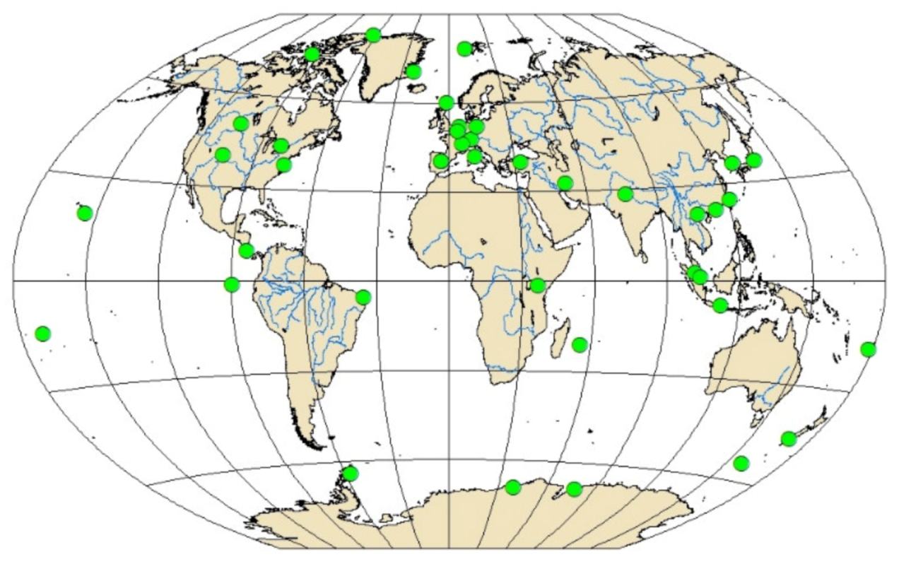
Ozonesonde data used in the study were obtained from WOUDC (Figure 1). The ECC and BM types for the ozonesondes are widely used at present. Stubi et al. demonstrated that there was no significant difference between ECC and BM of radiosonde at 90% confidence level [35]. Logan et al. [36] compared the radiosonde and the Measurements of Ozone and Water Vapor by In-Service Airbus Aircraft (MOZAIC) data in Frankfurt and Munich from 1999 to 2008, and showed that the average ozone deviation in the lower troposphere (681~580 hPa) was 0.9 ± 2.8 ppb, and the deviation was 1.7 ± 3.8 ppb at 501–430 hPa. In general, the ozone profiles data of WOUDC were sufficiently accurate, and could be used as the reference for satellite and other observation methods (WOUDC, 2007). In this study, 20 sounding stations were selected across the Northern Hemisphere from 2014 to 2020 (as shown in Table A1).
2.1.2. CARIBIC Flights Data
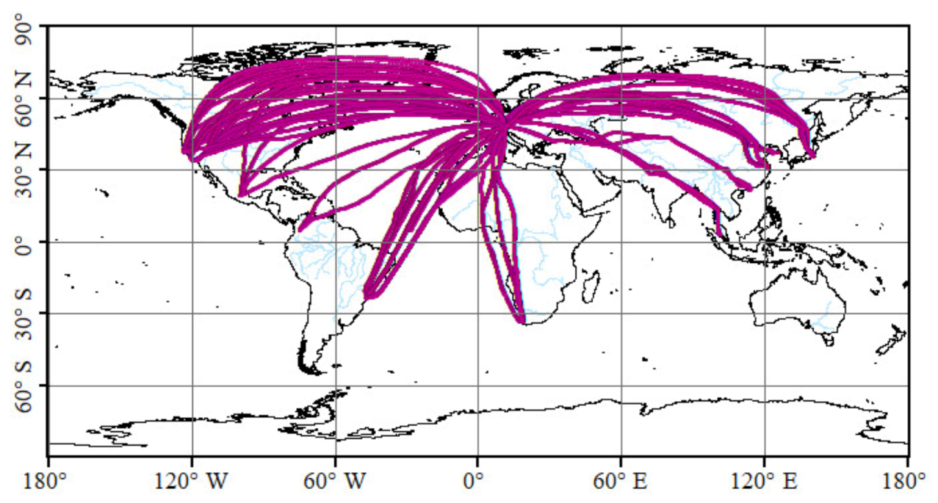
CARIBIC is a scientific project that studies and monitors the important chemical and physical processes of trace gases and other components in the Earth’s atmosphere with a 1 s time resolution. The Northern Hemisphere data from CARIBIC synthesized in 2 min intervals from January 2014 to December 2020 were chosen in this study. The container of CARIBIC is operated monthly on flights from Germany to the Americas, Asia, and Africa. Only in a few flights is the Southern Hemisphere is probed. Flight data ranging from 2014 to 2019 were collected in different locations within a narrow spectrum of altitudes. Each flight covers a wide range of areas, such as tropical middle tropospheric air or middle and high latitudes upper tropospheric air and lower tropospheric air [37]. In the tropics, the plane flies in the free troposphere, whereas in the extratropics, this altitude range corresponds to the tropopause region, and the aircraft frequently encounters stratospheric air masses. The container on the flight includes the equipment for in situ measurements of greenhouse gases (carbon dioxide, nitrogen oxides, and methane) including ozone, water vapor, carbon monoxide, dust particles, and many more. Air sampling is carried out at cruise altitude, and more than 99% of the samples are collected at a typical pressure altitude of 230 ± 60 hPa. Comparisons with a laboratory standard showed that ozone measured with a UV photometer at a time resolution of 4 s can achieve a precision of 0.3 ppb and a total uncertainty of ~1.5% [38]. Figure 2 shows the selected CARIBIC flights data from 2014 to 2019.
2.1.3. Near-Surface Ozone Data
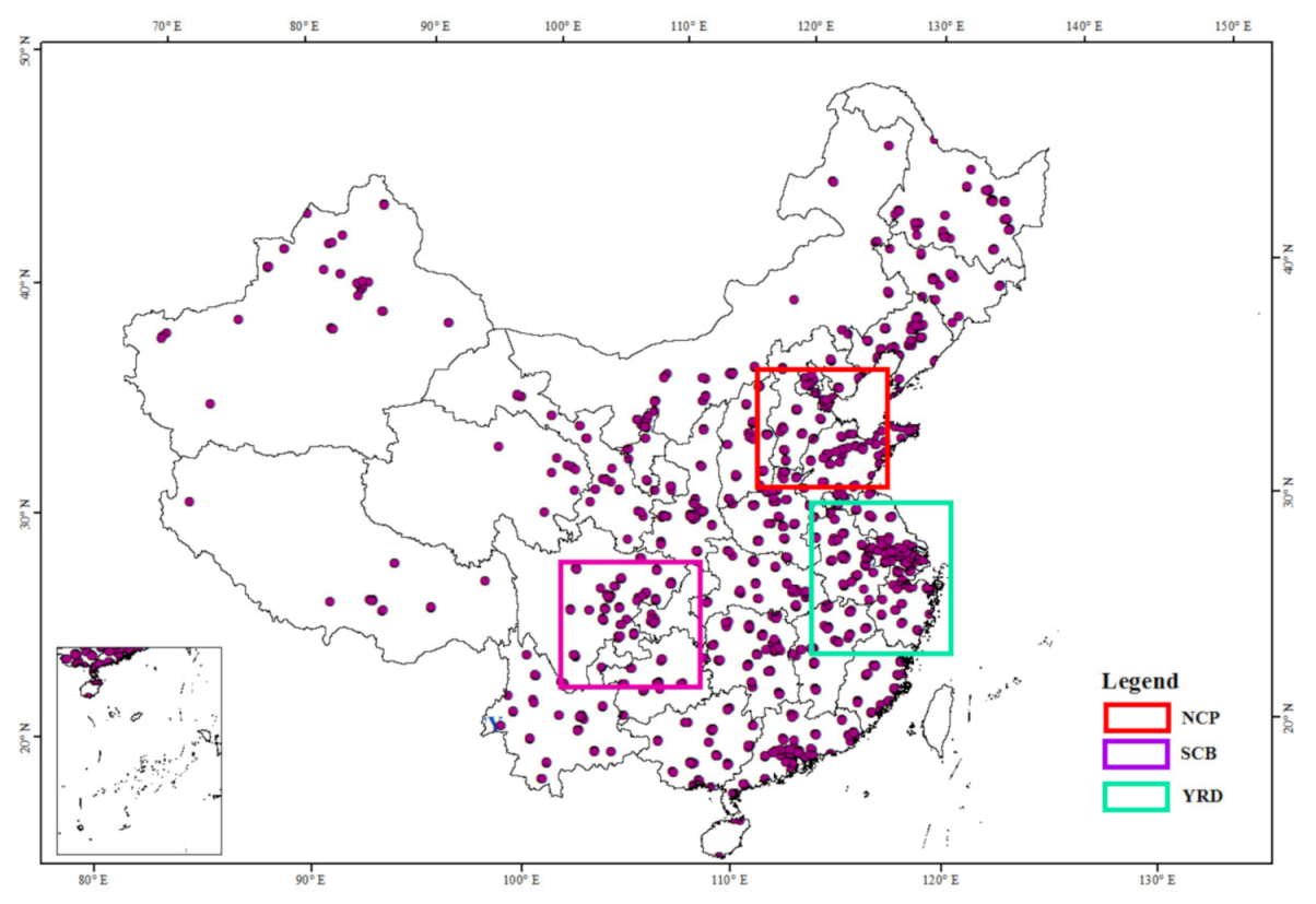
China’s continuous observation of near ozone concentrations began in 2005 [39]. The hourly data of near-surface ozone concentrations online in real time are reported by China Environmental Monitoring Center (CNEMC, http://www.cnemc.cn, accessed on 1 February 2021), but it is still not possible to obtain the historical ozone data from the network publicly. There may be errors and suspect values in the data of CNEMC. Therefore, the quality control test was carried out through a quality assurance program. Near-surface ozone data (1000 hPa is regarded as the surface pressure) in three typical areas (Figure 3) of China were selected for validating the accuracy and generalizability of the model, which are of great concern to the public, including the Sichuan Basin (SCB), North China Plain (NCP), and Yangtze River Delta region (YRD). Hourly (13:00–14:00) in situ surface ozone observations at monitoring stations (139, 240, and 331 uniformly distributed surface ozone monitoring stations in SCB, NCP, and YRD, respectively) acquired by the China National Environmental Monitoring Center (CNEMC) of three typical areas from January 2017 to December 2019 were collected.
2.2. Satellite Data
Satellite data were taken from AIRS and OMI onboard the Aqua and Aura, respectively. The AIRS sounder onboard of NASA’s Aqua platform provided us with the capability to retrieve daily ozone data over land, ocean, and polar regions during the day and night. This study used the Aqua L2 product—AIRS Cloud-Cleared Radiances (CCRs) [40]. The CCRs employed the cloud-clearing method that removed the cloud from an infrared cloudy field of view and derived the cloud-cleared radiances, with a spatial resolution of 50 km. The parameters in the Aqua L2 product are the radiance of seven channels near the absorption band of 9.6 μm, together with geographic information related to the solar azimuth angle, solar zenith angle, satellite zenith, and azimuth angle. OMI is an ozone monitor on the Aura satellite with a spectral range of 0.27–0.5 μm. In this study, the apparent reflectance (ρ) was calculated using 15 channels in the spectral radiance band of 310–340 nm (ozone absorption band) and the average solar spectral irradiance was provided by OMI:
where ρ is the apparent reflectance, π is 3.1415, L is the spectral radiance of the satellite sensor entering the top of the atmosphere, D is the distance between the Sun and the Earth, ESUN is the average solar spectral irradiance at the top of the atmosphere, and θ is the solar zenith angle. The spectral radiance and irradiance of OMI were taken from the Aura L1B product, with a spatial resolution of 13 km × 24 km. Both L and ESUN were provided by OMI. According to the temporal and spatial information of ozone data, coincident satellite data were extracted.
2.3. Meteorological Data
The meteorological data were taken from ERA5 reanalysis data. ERA5 is the fifth- generation climate reanalysis dataset of the European Centre for Medium-Range Weather Forecasts (ECMWF) [41,42], with a spatial resolution of 25 km and a 1 h resolution. Ten meteorological factors with 27 pressure levels in 1000–100 hPa, i.e., the divergence (d, unit: s−1), fraction of cloud cover (CC), potential vorticity (PV, unit: K m2 kg−1 s−1), relative vorticity (VO, unit: Pa s−1), temperature (T, unit: K), specific humidity (q, unit: kg/kg), vertical velocity (w, unit: Pa s−1), eastward component of wind (U, unit: m s−1), northward component of wind (V, unit: m s−1), and relative humidity (r, unit: %) at a 0. 25° × 0.25° resolution were used in this study. In addition, the input data also include the time (year, month, day, and hour) and geographic location information (geo, including latitude and longitude). We extracted the matching ERA5 meteorological data based on the time and space information of LST ozone data.
2.4. Dataset Used and Processing
Table 1 presents detailed information about the selected datasets. Because the datasets used in the study have different spatial and temporal resolutions, all data sets were uniformly resampled to the same spatial size (0.25° × 0.25°) using the bilinear interpolation method and the same time interval. The meteorological variables selected (d, CC, PV, VO, T, q, w, U/V, and r), the radiance of seven channels near the ozone absorption band from AIRS CCRs, the apparent reflectance of 15 channels from OMI and time, and geographic location information were matched to the daily LST ozone concentrations for each station. All the datasets used were uniformly resampled to the same vertical grid based on the ERA5 pressure.
3. Methods
3.1. Variable Analysis
LST ozone is affected by many factors. The strong solar radiation and long duration of sunshine are generally assumed to lead to the photochemical generation of ozone [43]. In addition to the these factors, the pressure (P) closely related to the atmospheric circulation and synoptic-scale meteorological pattern is also recognized as a main driving force for the ozone concentration over the Northern Hemisphere [44]. The U/V-component of wind (U/V) is widely used to capture the influence of wind on air pollutants over a certain period of time. The ozone concentration also relies on temperature. As depicted in many studies, a high ozone concentration correlates with high temperature [45]. Relative humidity (RH) affects heterogeneous reactions of ozone and particles [46,47]. Potential vorticity (PV) reflects the stratospheric tropospheric exchange, and the main reason for the cause of this is the change of tropopause. The vertical velocity (W) at different pressure levels can provide information on the ability of low-pressure systems to transport air masses vertically by convection [48]. Relative vorticity (VO) is a measure of the rotation of horizontal air around a vertical axis relative to a fixed point on the Earth’s surface.
According to the previous research on the influence factors of LST ozone, we use the random forest [49] method to analyze the importance of the factors affecting LST ozone. Recently, the variable importance measures yielded by random forests have also been suggested for the selection of relevant predictor variables in the analysis of microarray data and other applications. The “mean decrease accuracy” method of random forest [50] was applied in this study. The method determines the variable importance by directly measuring the influence of each feature on the prediction accuracy of the model. The basic idea of the method is to add a random noise to a certain eigenvalue, and then observe the degree to which the accuracy of the prediction is reduced. For the unimportant features, this method has little influence on the prediction accuracy of the model, but for the important features, it will greatly reduce the prediction accuracy of the model. The data used were meteorological data, satellite data, latitude, longitude, and time matched with WOUDC LST ozone data from 2014 to 2020. The LST ozone data were from WOUDC, taken from 2014 to 2020. The specific steps follow to determine the benchmark value of prediction accuracy in the training model:
- (1)
- Add a random noise to the variable X (temperature, humidity, and so on), and the prediction accuracy of the model was recalculated. If the prediction accuracy of the model is greatly reduced after adding the noise, then it is of high importance.
- (2)
- Repeat for all variables to calculate the variable importance.
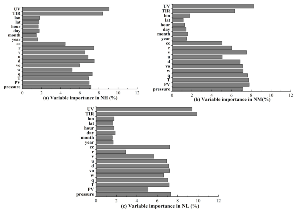
Because of the obvious difference of ozone with latitude and season, in this study we divided the Northern Hemisphere into three regions according to latitude for characteristic importance analysis: Northern Hemisphere at low latitude (0–30°N, NL), Northern Hemisphere at middle latitude (30°N–60°N, NM), and Northern Hemisphere at high latitude (60°N–90°N, NH). The results showing the variable importance of input parameters are shown in Figure 4. In the three different regions, the meteorological variables collectively account for more than 50% of the overall relative importance. Temperature, specific humidity, relative humidity, divergence, vertical velocity, vorticity, and the U/V-component of wind are the predominant variables. The high importance of meteorology for tropospheric ozone has also been found in several studies [20,51]. Following the meteorological factors, UV and TIR serve as the main factors for predicting the Lower-Stratosphere-to-Troposphere ozone values. Although variables importance results show that time (year, month, day, and hour) and geographic information (latitude and longitude) are not the most important factors affecting LST ozone concentrations, geographical and seasonal changes are still indispensable factors affecting LST ozone concentrations [52].
3.2. LSTM Model
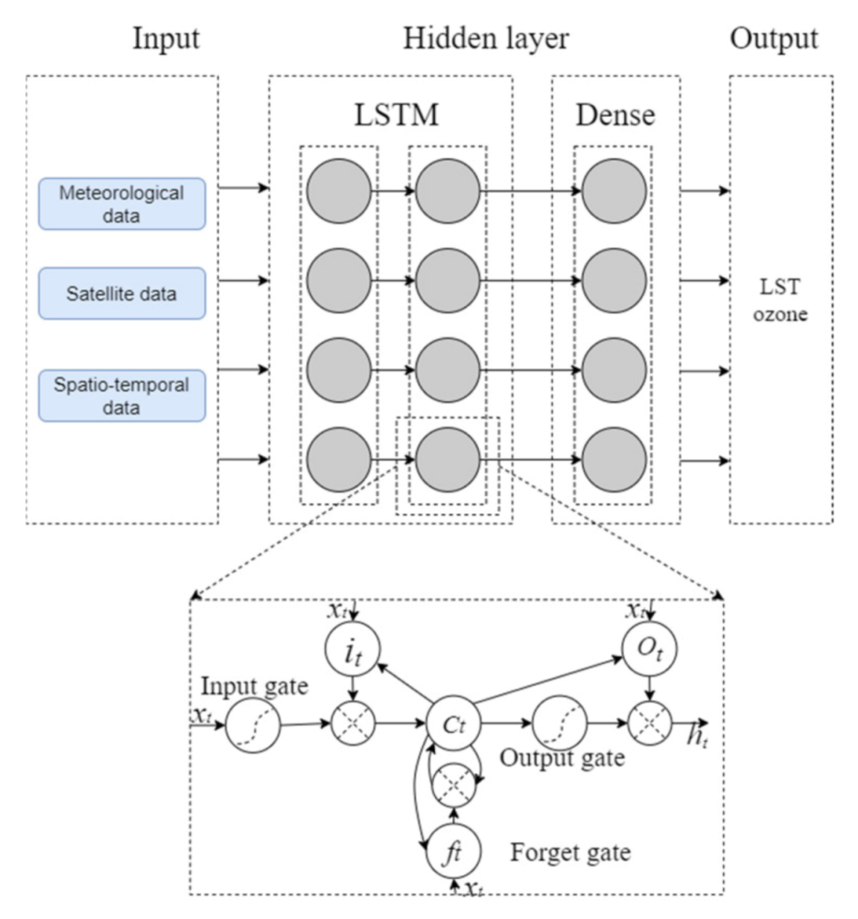
LSTM optimizes the problems of gradient vanishing and gradient explosion in Recurrent Neural Networks (RNNs), and is an effectively optimized network with the ability to memorize the sequence of data and to deal with sequential pattern recognition problems [53]. The basic unit for a common LSTM is a memory cell composed of three gates: an input gate, an output gate, and a forget gate. An adaptive “forgetting gate” enables the LSTM network to learn automatically and judge whether to store memory information. The cell state carries all the previous state information and the cell state will be adaptively adjusted with the new states by discarding the old information or adding information. Figure 5 shows the LSTM neurons, which include the input gate it, forgetting gate ft, unit Ct, output gate Ot, and output response ht. The input gate and forgetting gate control the inflow and outflow of information. The output gate controls the amount of information from the unit to the output ht. Supposing W is the weight vector of a gate and b is the bias value, then the gate can be expressed as Equation (2):
where σ is the activation function, and bi, bf, and bo are it, ft, and Ot bias values, respectively. Figure 5 is the structure of our model used to predict the LST ozone. In a series of experiments, three layer types were applied to predict LST ozone: the input layer with LSTM, hidden layers (the first two hidden layer were LSTM, the third hidden layer was the dense layer), and the output layer with the dense layer. The input layer of the module accepted three kinds of datasets: meteorological variables, satellite radiances/apparent reflectance parameters, and spatial temporal information. Because of the different samples in different regions of the Northern Hemisphere, the number of neurons in each layer was typically set manually, and the best composition was problem-specific. The numbers of the input layer’s neurons at NH, NM, and NL were 40, 60, and 40, respectively. The numbers of neurons in hidden layers of NH, NM, and NL were 20–10–10, 20–10–10, and 30–15–15, respectively. The output is the LST ozone profile concentrations.
In order to improve the training accuracy and speed up the convergence of the module, the z-score standardization method was used to transform the input data, with the mean value of 0 and the standard deviation of 1. The z-score function [54] is given as follows:
where x is the input data, μ and σ are the mean value and standard deviation value of x, respectively. The model adopted the default activation function Tanh in the input layer. The Tanh is a smoother zero-centered function whose range lies from −1 to 1. The hidden layers used the activation function ReLU, which was able to speed up the learning convergence [55]. The activation functions Tanh and ReLU are given in Formulas (7) and (8), respectively. The learning rate, as an important hyperparameter in deep learning, determined whether the objective function converged to a local minimum and the speed at which it converges to the minimum. A proper learning rate can make the objective function converge to a local minimum in a reasonable time. In this study, we employed the LearningRateScheduler [56] function, which can automatically adjust the learning rate according to the number of epochs. At the beginning of training, a high learning rate was used to increase the convergence and training speed; we then gradually reduced the learning rate to reduce the overfitting and improve the training accuracy. The learning rate was reduced to 0.5 of the original in every 100 epochs. When training the model, we used the RMSprop [57] optimizer with a batch size of 72 to minimize the cost function. The output layer that adopted the dense layer produced the LST ozone profiles.
In order to reflect the performance of the model, in this paper, we used the correlation coefficient (R2), mean root mean square error (RMSE), and mean absolute error (MAE) to evaluate the performance of the model. The implementation of the model was based on Keras, which is a high-level neural network application programming interface written in Python.
where is the predicted value, is the average value of predicted values, is the observation value, and is the average value of observation values.
4. Results
In this section, Section 4.1 describes the trained models at NH, NM, and NL, and the trained models are applied to the same data source (WOUDC) at different times. In order to further prove the generalizability of the model, the trained models were applied to different data sources (CARIBIC and CNEMC), as shown in Section 4.2.
4.1. Model Training
In this section, the LST ozone data of the trained model taken from WOUDC are presented. The module was trained, validated, and tested in three different regions using a history of all observed parameters (ERA5, satellite data, and WOUDC ozone profiles) from 2014 to 2020—the data from 2014 to December 2017 were used for training (80% of total data), the data from January 2018 to December 2018 were used for validation (10% of total data), and the data from January 2019 to December 2020 were used as the test set (10% of total data). The reason why WOUDC datasets were divided into three parts is that the training sets were used to train the LSTM modules, the validation sets were used to adjust hyperparameters during training, and the testing sets were used to objectively evaluate the performance of the model.
Table 2 shows statistical results of training, validation, and test from ozone concentrations in all pressures. As shown in Table 2, the number of samples is smaller than that of corresponding profiles multiplied by 27 due to missing values in some pressures. However, to analyze the overall performance of the model, we compute the R2, root mean square error (RMSE) and the mean average error (MAE) in NH, NM, and NL by using ozone concentrations in all pressures. The results illustrate that the R2 values of the training set in NH, NM, and NL were 0.978, 0.905, and 0.695, respectively, and the R2 values of the validation sets in NH, NM, and NL were 0.936, 0883, and 0.612, respectively. The R2 of the training model was highest in NH, but the RMSE and MAE of the training model in NL were low, at 20.640 and 13.085 ppb, respectively. The RMSE of the training model in NH and NM was 86.921 and 68.042 ppb, and the MAE was 34.847 and 31.013 ppb, respectively. In total, 1909, 7780, and 1933 test samples were collected from NH, NM, and NL respectively. The model in NH performed well, with a high R2 equal to 0.905, RMSE of 94.222 ppb, and MAE of 36.348 ppb. The mean R2, RMSE, and MAE in NM and NL were 0.885 and 0.590, 71.110 ppb and 20.153 ppb, 29.079 and 13.322, respectively. The training models performed differently in the three regions, mainly due to significant variations in climate conditions.
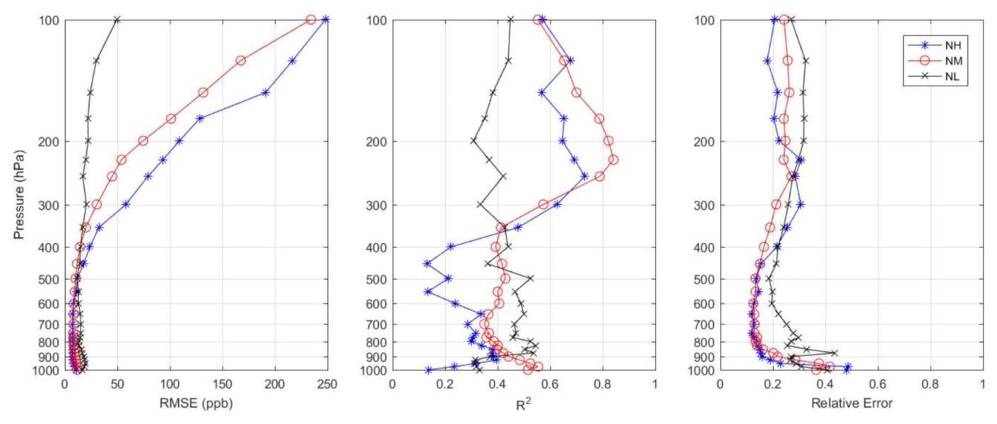
Figure 6 shows the testing samples of mean RMSE, R2, and Relative Error (RD) stratification of LST ozone for the test sets ranging from 2019 to 2020 in different latitudes (NH, NM, and NL). RD can be expressed by Formula (12):
The RMSE in NH and NM increased with the increase of altitude, to a maximum of 100 hPa. While the RMSE in NL showed little change with the altitude, and the RMSE in each pressure was less than 50 ppb. Particularly, the maximum R2 of each layer in NH was 250 hPa, which was greater than 0.7. The R2 of each layer in NL was almost in the range of 0.3–0.6. The R2 values of each layer in NM were almost in the range of 0.36–0.85, and the maximum R2 happened in 225 hPa. The RD stratification values of each layer on the test sets were larger at 850–1000 hPa in the three different latitudes. The mean RD of all pressures from 100 to 1000 hPa in NH, NM, and NL were 0.217, 0.23, and 0.278, respectively.
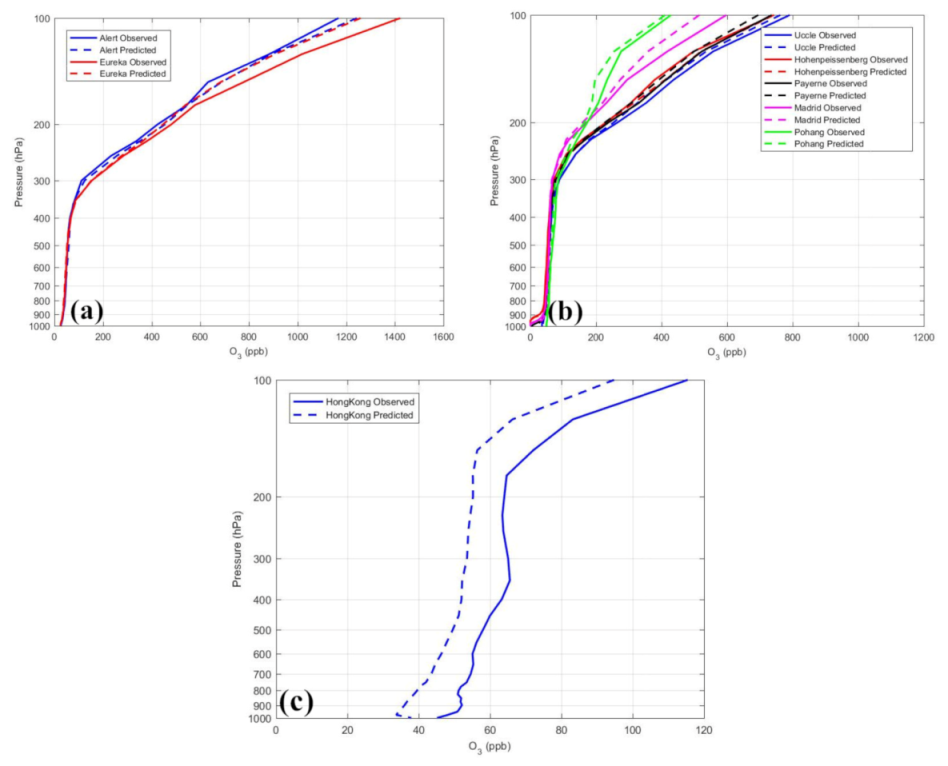
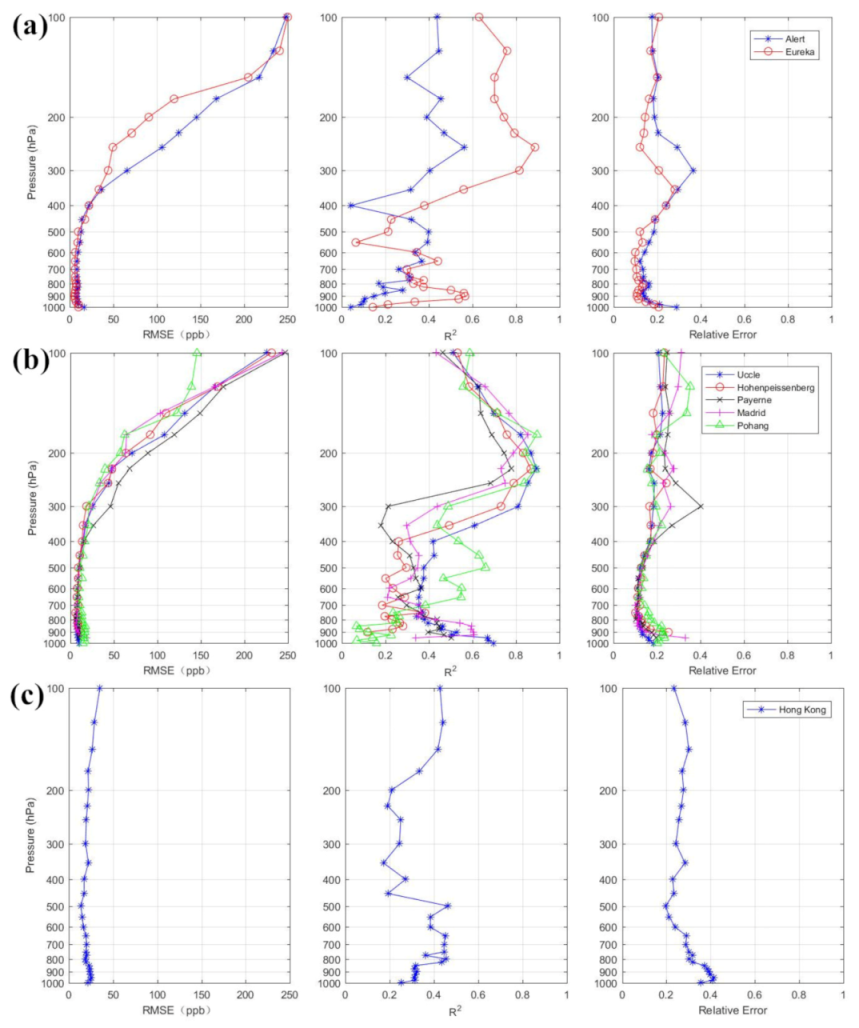
Figure 7 shows the mean of vertical concentrations of LST ozone on the test sets at eight WOUDC stations since 2019. We can see that the predicted LST ozone profiles are consistent with the observations, while the predicted values are generally lower than the observations. Figure 8 shows the RMSE, R2, and relative error of WOUDC stations, since 2019 was at different pressures. The RMSE of these stations in NH and NM increased with altitude, while the RMSE of Hong Kong in NL showed little change at different pressures. It is seen from Figure 8 that the correlations between the prediction results and observations above 400 hPa at most stations in NH and NL regions are greater than that of 400 hPa. This is because the influencing factors of tropospheric ozone are different in different pressure layers. The LST ozone concentrations may be affected by meteorological factors above 400 hPa in a large extent, and below 400 hPa due to photochemical reactions, a precursor, which make ozone changes more complex; the ozone precursors are not trained in the model. This is also the reason why the results of the model in the middle and lower troposphere are generally worse than those in the middle and upper troposphere. The R2 of Hong Kong in NL changes little at different pressures, with a R2 = 0.2~0.4. The performance of Hong Kong stations is different with the stations in NH and NM; this may be due to the tropospheric ozone in Hong Kong being affected by the increase in photochemical production, and the increase in transboundary transport [58].
4.2. Model Evaluation
In order to improve the model’s accuracy, we migrated the trained model to different regions and verified it with ozone data from different data sources. Different data sources have invisible characteristic information such as region and special climate. The larger the information gap between data sources, the greater the difference of these invisible characteristics, and the greater the difference of ozone distribution. In this case, applying models that were pretrained on other data sources may lead to the inapplicability of feature information. Therefore, the model needed to be migrated in order to learn some implicit features of the new data. In this section, we present the fine-tuning of the LSTM models presented in Section 4.1.
4.2.1. Applied to CARIBIC
The CARIBIC flights data, with typical pressure of 230 ± 60 hPa, were matched with the pressure of ERA5. Most of the matched data were distributed at 200, 225, 250, and 300 hPa. The CARIBIC flights data chosen, ranging from January 2014 to February 2019 in NH, NM, and NL, were divided into a pretraining part (2014–2017) and a fine-tuning part (January 2018–February 2019), respectively. Table A2 shows the prediction performance of the migration models on CARIBIC flight data from January 2018 to February 2019 under different hidden frozen layers [59] in NH, NM, and NL. To freeze a layer means that it excludes the layer from the training process. The process of the transfer training is performed by using the weight parameters of trained models in Section 4.1, and keeping the weight parameters of the frozen layer unchanged to train the migration model. This was done to observe the predictive performance of the model with different frozen hidden layers ((0), (1), (1,2), and (1,2,3)). We can see that the transfer model of NH and NM with the hidden frozen layers (1,2) achieved a higher R2 (0.774 and 0.443, respectively), and a lower RMSE (77.410 and 109.334 ppb, respectively) and MAE (92.978 and 72.932 ppb, respectively). The transfer model of NL with the different hidden frozen layers did not change greatly, with an R2 = 0.359, RMSE = 17.972 ppb and MAE = 17.061 ppb, respectively, in hidden frozen layers (1). The R2, RMSE, and MAE in Table A2 were calculated by using the ozone concentrations from all pressures in the pretraining part.
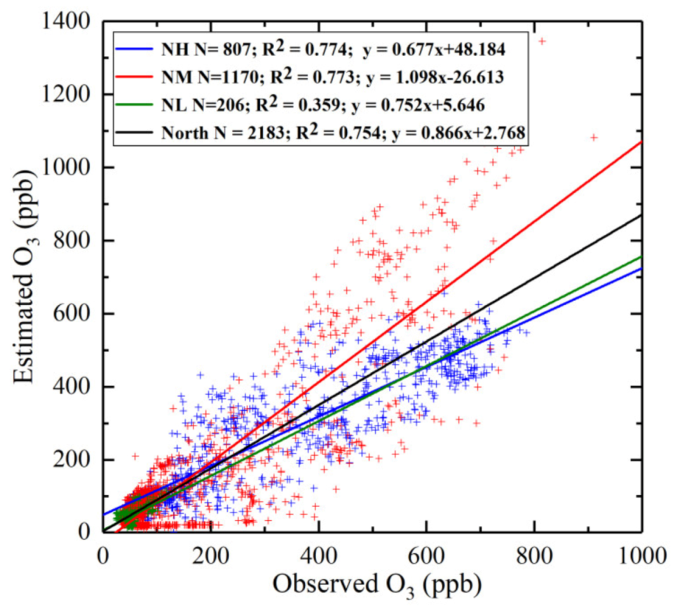
Figure 9 displays the comparison results of the CARIBIC flight data that ranged from January 2018 to February 2019 with a pressure 200–300 hPa derived from LSTM and aircraft measurements. The N in Figure 9 represents the number of samples used to evaluate the tropospheric ozone estimation performance. The R2, RMSE, and MAE in Figure 9 were calculated by using the LST ozone profiles at each pressure in NH, NM, and NL of the fine-tuning part. Overall, the LST ozone derived from the migration model agrees well with the CARIBIC measurements; the model presents good results in the Northern Hemisphere, with a high R2 = 754. The performance of the models in NH and NM were overall better (e.g., R2 ≈ 0.770) than in NL (with an R2 = 0.359). The factors affecting tropospheric ozone in NL are complex. This may be due to the redistribution of ozone concentration caused by the thermal and dynamic forcing of atmospheric circulation in NL.
4.2.2. Applied to CNEMC
This part focuses on evaluating the predictability of the trained models in three urban agglomerations of China. For this purpose, the prediction of surface ozone of three typical areas (Figure 3) was validated using the data provided by CNEMC. Hourly (13:00–14:00) in situ surface ozone observations at monitoring stations of three typical areas from January 2017 to December 2019 were collected and then averaged to obtain daily mean ozone measurements. The matched CNEMC data of three urban agglomerations from January 2017 to December 2019 were divided into a pretraining part (2017) and a fine-tuning part (2018–2019), respectively. The transfer model used in SCB was trained based the model in NL, with the hidden frozen layers (1,2) performing better, and the best results can be seen in Figure 10a. The transfer model used in NCP was trained based on the model in NM, with the hidden frozen layers (1,2) showing better achievement, and the best results can be seen in Figure 10b. The transfer model used in YRD was trained based on the model in NL, with the hidden frozen layers (1,2,3) performing better, and the best results can be seen in Figure 10c.
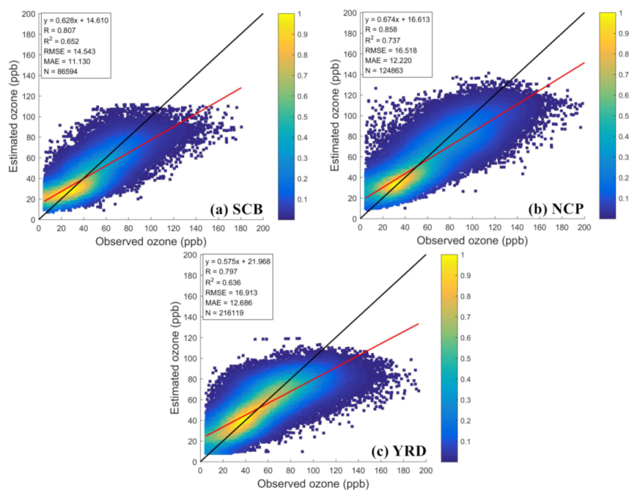
Figure 10 shows the predicted and observed daily surface ozone distribution in SCB, NCP, and YRD. There were 86,594; 124,863; and 216,120 daily samples collected from surface ozone monitoring stations in SCB, NCP, and YRD, respectively. The daily estimated ozone concentrations in the typical urban agglomerations of the SCB, NCP, and YRD were consistent with surface measurements (R2 = 0.652−0.737), with overall estimation uncertainties (i.e., an RMSE = 14.543−16.916 ppb and MAE = 11.130−12.687 ppb) from 2018 to 2019. The performances of LSTM showed slight differences for each year during 2018~2019 in the three typical urban agglomerations. As shown in Table 3, the R2 value showed the highest value (0.706) in NCP in 2019, followed by that in 2018 (0.747), and showed the lowest value in SCB (0.648 in 2018 and 0.670 in 2019) and YRD (0.621 in 2018 and 0.650 in 2019). Higher RMSE and MAE values were found in NCP (15.881–17.157 ppb and 11.734–12.720 ppb) and YRD (16.207–17.764 ppb and 12.134–13.276 ppb), while the lowest RMSE and MAE were found in SCB (14.194–14.930 ppb and 10.783–11.496 ppb). The lowest R2 value being in SCB might be attributable to meteorological factors. The variation of surface ozone concentration in SCB was greatly affected by the high annual temperature, seasonal cycle, small wind speed, mostly static wind, short sunshine time, and obvious seasonal heat island effect and meteorological conditions (such as high temperature, low humidity, low wind speed, and long sunshine time) [33], which have a greater comprehensive effect on high concentrations of ozone. We also find outliers of high surface ozone concentrations that were underestimated by the model. The underestimation of the predicted ozone largely depended on the number, geographical distribution, and sampling frequency of training samples, which did not cover mainland China (except for the Hong Kong and Taiwan sites) and the sparsity of training samples on the surface.
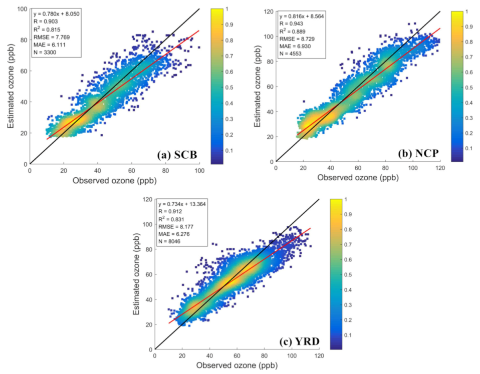
Based on the prediction results for near-surface ozone of three urban agglomerations presented above for the period of 2018–2019 at the daily scale, we conducted a statistical comparison of results at the monthly scale. When considering the monthly scale, the stations with >15% of valid daily surface ozone concentration measurements in a month were used in the calculations. Figure 11 shows the cross-validation results for surface ozone monthly estimates from 2018 to 2019 in China. From 2018 to 2019, each site had at least eight months of effective monthly averages to be counted. Figure 11 shows that the predicted values of surface ozone were highly correlated with the observations. The accuracy in NCP was 0.889, 8.729 ppb, and 6.930 ppb for R2, RMSE, and MAE, respectively. The monthly ozone estimations performed better than the daily estimations in SCB and YRD regions (i.e., R2 = 0.815, MAE = 6.111 ppb and RMSE = 7.769 ppb in SCB, R2 = 0.831, MAE = 6.276 ppb, and RMSE = 8.177 ppb in YRD). Overall, despite some differences in the three clusters’ performance, the LSTM model showed overall good prediction accuracy for surface ozone concentrations at the regional scale on monthly averages.
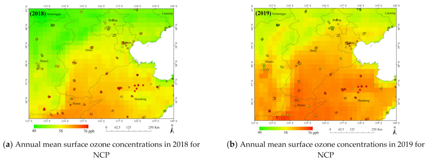
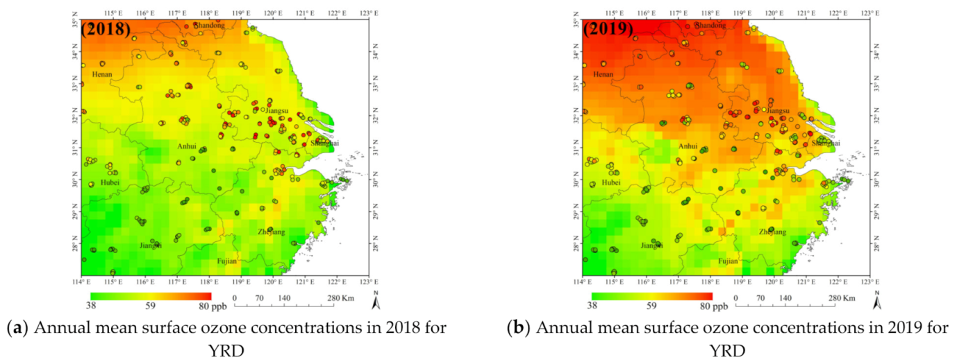
Figure 12, Figure 13 and Figure 14 show the 0.25° × 0.25° spatial distributions of the migration models applied above in the three typical areas and the ground-based surface ozone measurements for 2018–2019. Figure 12 shows annual surface ozone spatial distributions across SCB for 2018 and 2019. The model in SCB has a good performance in areas with low values of ozone, but the areas with high ozone concentrations are underestimated. We see that the surface ozone concentrations of eastern Sichuan and western Chongqing are higher than other parts in Figure 12. It is obvious that the annual mean surface ozone concentrations in 2019 for North Central Hebei, most of Shandong, and southern Shanxi are higher than those in 2018, which are consistent with the trend of the ground-based observations in NCP (Figure 13). The evaluation of the model in YRD performs well in areas with low ozone values, such as Jiangxi Province and southern Zhejiang Province (Figure 14). We also can see the surface ozone concentrations for northern YRD in 2019 are larger than those in 2018. The performance of the model in the south of Jiangsu Province is poor, however, and the ozone concentrations in northern YRD are higher than other parts in YRD.
5. Discussion
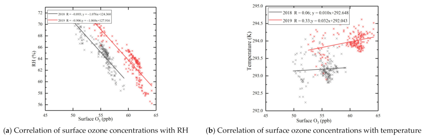
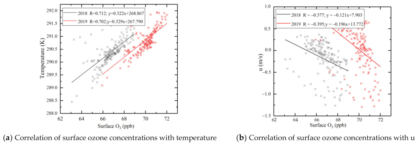
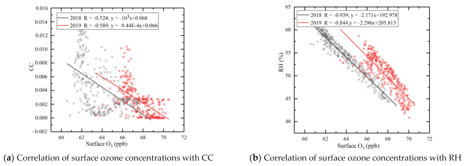
In this study, we considered the meteorological and radiance factors that affect LST ozone. Because LST ozone is also affected by a photochemical reaction, LST ozone is also affected by NO2, HCHO, CHOCHO, and other precursors. However, at present, there is almost no profile information for ozone precursors, so the influence of gas precursors was not considered in this study. The models trained in this study were applied to three typical urban agglomerations in China to predict surface ozone concentrations. It could be seen that the prediction results were generally underestimated. This may be due to the ozone at 1000 hPa of WOUDC stations being lower than that at 1000 hPa of the China regions, and LST ozone not fully representative of surface ozone. Figure 12, Figure 13 and Figure 14 show the spatial distributions of the migration models applied in SCB, NCP, and YRD for 2018–2019. Based on the input of the model, we analyzed the influencing factors of the high value of ozone. Figure 15, Figure 16 and Figure 17 list the input parameters with high ozone correlation. The surface ozone concentrations of eastern Sichuan and western Chongqing are higher than other parts in SCB. This may be caused by high temperature and low humidity [60]. Figure 15 shows the correlation of surface ozone concentrations with temperature and RH in eastern Sichuan and western Chongqing from 2018 to 2019. We can see that ozone concentrations are positively correlated with temperature and negatively correlated with relative humidity. Moreover, the absolute values of correlation of surface ozone concentrations with temperature and RH in 2019 are higher than those in 2018. This also shows that high temperature and low humidity are the factors affecting ozone concentrations. The ozone concentrations in southern of NCP are higher than other parts in NCP. Figure 16 shows the correlation of surface ozone concentrations with temperature and u in the southern of NCP (36°–38°N, 114°–118°E) from 2018 to 2019. We can see that ozone concentrations are positively correlated with temperature and negatively correlated with u. Cloud cover and low humidity are also the main factors affecting ozone concentrations in YRD. The ozone concentrations in the northern part of YRD are higher than other parts of YRD. Figure 17 shows the correlation of surface ozone concentrations with CC and RH in the northern part of YRD (32°–34°N, 116°–119°E) from 2018 to 2019. We can see that ozone concentrations are negatively correlated with CC and RH. Cloud cover and low humidity are also the main factors affecting ozone concentrations in YRD.
6. Conclusions
With the increase of atmospheric ozone pollution in recent years, a large number of studies focusing on estimating tropospheric ozone have been conducted. Traditional methods also face great challenges of tropospheric ozone estimates due to large uncertainties in the retrieval as it is influenced by numerous factors. In order to tackle these challenges, LSTM models are proposed to estimate lower-stratosphere-to-troposphere ozone concentrations from 100 hPa to the surface. In this study, three models were trained to estimate the ozone concentrations in the Northern Hemisphere. The training models in NH, NM, and NL perform well, giving high R2 values of 0.978, 0.905, and 0.695, respectively. The model performance was evaluated using the data of WOUDC ranging from 2019 to 2020 in different latitudes, CARIBIC flight data from 2018 to 2019, and in situ surface ozone observations at monitoring stations of three typical areas (SCB, NCP, and YRD) in China from January 2018 to December 2019.
By applying the models to the validation sets of WOUDC data of 2019–2020, the results in NH and NM were shown to perform well (R2 = 0.928 and 0.885, respectively), while the R2 = 0.590 in NL was lower than NH and NM. However, the RMSE value of NL was smaller than the other regions, probably because the NL region has a small range of tropospheric ozone. Meanwhile, the LSTM models were applied to the CARIBIC flights data, with a high precision of R2 = 0.881 and RMSE = 52.402 ppb. Finally, the models were applied to estimate the tropospheric ozone of the three typical urban agglomerations of the SCB, NCP, and YRD from 2018 to 2019. Our results suggest that the performance of the LSTM models showed a good estimation of the monthly surface ozone concentrations in all the three clusters, with a relatively high coefficient of 0.815−0.889, RMSE of 7.769−8.729 ppb, and MAE of 6.111−6.930 ppb. The daily scale performance was not as high as the monthly scale performance, with an accuracy of R2 = 0.636−0.737, RMSE = 14.543−16.916 ppb, MAE of= 11.130−12.687 ppb. The ozone concentrations in SCB might be affected by the high annual temperature and relative humidity. The overall predicted surface ozone concentration of our models was underestimated compared to the observations. The underestimation of the predicted ozone largely depends on the number of training samples and the sampling frequency. The distribution of the retrieval lower-stratosphere-to-troposphere ozone concentrations can be conducive to the study of ozone transportation and pollution in some small- and medium-scale regions, which is of great significance for the study of long-term ozone variation and its causes.
Author Contributions
Conceptualization, X.Z., Y.Z. and L.C.; formal analysis, X.Z., Y.Z. and L.Z.; funding acquisition, L.C., Y.Z., J.T., X.L. and Z.W.; methodology, Y.Z.; supervision, Y.Z. and L.B.; visualization, X.Z.; writing—original draft, X.Z.; writing—review and editing, X.Z., Y.Z. and L.B. All authors have read and agreed to the published version of the manuscript.
Funding
This study is supported by the National Natural Science Foundation of China (Grant No. 91644216, 41771391), National Key Research and Development Program of China (2018YFC0213903, 2018YFC0213904), Strategic Priority Research Program of the Chinese Academy of Sciences (Grant No. XDA19010403, XDA19040201), Guangxi Key Research and Development Project (Grant No. Guike AB20238015), TUOHAI special project (Grant No. HBHZX202002) 2020 and the project of Excellent and Middle-aged Scientific Research Innovation Team of Northeast Petroleum University (Grant No. KYCXTD201903).
Acknowledgments
Thanks given for the in situ ozone ground-measurements used in this study that were available from the China National Environmental Monitoring Center, the OMI and AIRS data at Level 1 provided by NASA (https://disc.gsfc.nasa.gov/datasets, accessed on 1 October 2020), ERA5 reanalysis data provided by ECMWF, the WOUDC data (https://woudc.org/data/, accessed on 1 October 2020), and the CARIBIC flight data (https://www.ecmwf.int/, accessed on 20 October 2020).
Conflicts of Interest
The authors declare no conflict of interest.
Appendix A

Table A1.
Information of ozonesonde stations.
| Site | Country | Latitude (°) | Longitude (°) | Height (m) | Days | Dates |
|---|---|---|---|---|---|---|
| Alert | Canada | 82.49 | −62.34 | 75 | 166 | August 2015 to April 2020 |
| Eureka | Canada | 79.98 | −85.04 | 10 | 312 | January 2015 to September 2020 |
| Resolute | Canada | 74.7 | −94.96 | 46 | 114 | April 2015 to November 2018 |
| United Kingdom | Great Britain | 60.14 | −1.19 | 84 | 143 | January 2015 to December 2016 |
| Legionowo | Poland | 52.41 | 20.96 | 96 | 203 | January 2015 to October 2019 |
| Bilt | Netherlands | 52.100 | 5.177 | 4 | 182 | January 2015 to December 2018 |
| Uccle | Belgium | 50.8 | 4.35 | 100 | 768 | January 2015 to December 2020 |
| Hohenpeissenberg | Germany | 47.8 | 11 | 976 | 733 | January 2015 to December 2020 |
| Payerne | Switzerland | 46.49 | 6.57 | 491 | 781 | January 2015 to October 2020 |
| Vigna di Valle | Italy | 42.08 | 12.21 | 260 | 50 | January 2015 to November 2015 |
| Madrid | Spain | 40.47 | −3.58 | 631 | 315 | January 2014 to December 2020 |
| Boulder | USA | 39.9491 | −105.1 | 1743 | 144 | January 2015 to June 2017 |
| Tsukuba | Japan | 36.06 | 140.13 | 31 | 172 | April 2015 to February 2019 |
| Pohang | Korea | 36.03 | 129.38 | 6 | 97 | January 2018 to December 2019 |
| Taiwan | China | 24.9979 | 121.443 | 11 | 48 | January 2015 to March 2019 |
| Hong Kong | China | 22.31 | 114.17 | 66 | 294 | January 2014 to September 2020 |
| Hilo | USA | 19.43 | −155.04 | 11 | 187 | January 2015 to December 2017 |
| San Pedro | Costa Rica | 9.9396 | −84.0423 | 1240 | 156 | January 2015 to December 2017 |
| Sepang Airport | Malaysia | 2.73 | 101.7 | 17 | 68 | January 2014 to December 2017 |
| Singapore | Singapore | 1.34 | 103.89 | 36 | 18 | January 2014 to September 2015 |
Table A2.
Prediction performance of migration model under different frozen hidden layers of CARIBIC in NH, NM, and NL.
Table A2.
Prediction performance of migration model under different frozen hidden layers of CARIBIC in NH, NM, and NL.
| Frozen Layers | Region | R2 | RMSE (ppb) | MAE (ppb) |
|---|---|---|---|---|
| 0 | NH | 0.721 | 80.549 | 96.425 |
| NM | 0.727 | 112.301 | 76.264 | |
| NL | 0.354 | 18.012 | 17.956 | |
| 1 | NH | 0.741 | 79.256 | 94.821 |
| NM | 0.731 | 111.931 | 74.189 | |
| NL | 0.359 | 17.972 | 17.061 | |
| 1,2 | NH | 0.774 | 77.410 | 92.978 |
| NM | 0.773 | 109.334 | 72.932 | |
| NL | 0.352 | 17.523 | 17.496 | |
| 1,2,3 | NH | 0.769 | 78.736 | 93.648 |
| NM | 0.758 | 110.192 | 73.245 | |
| NL | 0.356 | 17.945 | 17.154 |
References
- Lelieveld, J.; Dentener, F.J. What controls tropospheric ozone? J. Geophys. Res. Atmos. 2000, 105, 3531–3551. [Google Scholar] [CrossRef]
- Rieder, H.E.; Polvani, L.M. Are recent Arctic ozone losses caused by increasing greenhouse gases? Geophys. Res. Lett. 2013, 40, 4437–4441. [Google Scholar] [CrossRef] [Green Version]
- Baasandorj, M.; Fleming, E.L.; Jackman, C.H.; Burkholder, J.B. O(D-1) Kinetic Study of Key Ozone Depleting Substances and Greenhouse Gases. J. Phys. Chem. A 2013, 117, 2434–2445. [Google Scholar] [CrossRef] [PubMed]
- Ma, P.; Chen, L.; Wang, Z.; Zhao, S.; Li, Q.; Tao, M.; Wang, Z. Ozone Profile Retrievals from the Cross-Track Infrared Sounder. IEEE Trans. Geosci. Remote Sens. 2016, 54, 3985–3994. [Google Scholar] [CrossRef]
- Young, P.J.; Naik, V.; Fiore, A.M.; Gaudel, A.; Guo, J.; Lin, M.Y.; Neu, J.L.; Parrish, D.D.; Rieder, H.E.; Schnell, J.L.; et al. Tropospheric Ozone Assessment Report: Assessment of global-scale model performance for global and regional ozone distributions, variability, and trends. Elem. Sci. Anth. 2018, 6. [Google Scholar] [CrossRef]
- Mills, G.; Buse, A.; Gimeno, B.; Bermejo, V.; Holland, M.; Emberson, L.; Pleijel, H. A synthesis of AOT40-based response functions and critical levels of ozone for agricultural and horticultural crops. Atmos. Environ. 2007, 41, 2630–2643. [Google Scholar] [CrossRef]
- Taylan, O. Modelling and analysis of ozone concentration by artificial intelligent techniques for estimating air quality. Atmos. Environ. 2017, 150, 356–365. [Google Scholar] [CrossRef]
- Ayres, J.G.; Ayres, J.; Maynard, R.L.; Richards, R. Air Pollution and Health; Imperial College Press: London, UK, 2006. [Google Scholar]
- Lupaşcu, A.; Butler, T. Source attribution of European surface O-3 using a tagged O-3 mechanism. Atmos. Chem. Phys. 2019, 19, 14535–14558. [Google Scholar] [CrossRef] [Green Version]
- Li, J.Y.; Mao, J.Q.; Fiore, A.M.; Cohen, R.C.; Crounse, J.D.; Teng, A.P.; Wennberg, P.O.; Lee, B.H.; Lopez-Hilfiker, F.D.; Thornton, J.A.; et al. Decadal changes in summertime reactive oxidized nitrogen and surface ozone over the Southeast United States. Atmos. Chem. Phys. 2018, 18, 2341–2361. [Google Scholar] [CrossRef] [Green Version]
- Li, R.; Cui, L.L.; Li, J.L.; Zhao, A.; Fu, H.B.; Wu, Y.; Zhang, L.W.; Kong, L.D.; Chen, J.M. Spatial and temporal variation of particulate matter and gaseous pollutants in China during 2014–2016. Atmos. Environ. 2017, 161, 235–246. [Google Scholar] [CrossRef]
- Li, X.; Zhang, Q.; Zhang, Y.; Zhang, L.; Wang, Y.X.; Zhang, Q.Q.; Li, M.; Zheng, Y.X.; Geng, G.N.; Wallington, T.J.; et al. Attribution of PM2.5 exposure in Beijing–Tianjin–Hebei region to emissions: Implication to control strategies. Sci. Bull. 2017, 62, 957–964. [Google Scholar] [CrossRef] [Green Version]
- Tan, Z.F.; Lu, K.D.; Dong, H.B.; Hu, M.; Li, X.; Liu, Y.H.; Lu, S.H.; Shao, M.; Su, R.; Wang, H.C.; et al. Explicit diagnosis of the local ozone production rate and the ozone-NOx-VOC sensitivities. Sci. Bull. 2018, 63, 1067–1076. [Google Scholar] [CrossRef] [Green Version]
- Liu, X.; Chance, K.; Sioris, C.E.; Spurr, R.J.D.; Kurosu, T.P.; Martin, R.V.; Newchurch, M.J. Ozone profile and tropospheric ozone retrievals from the Global Ozone Monitoring Experiment: Algorithm description and validation. J. Geophys. Res. Atmos. 2005, 110, 110. [Google Scholar] [CrossRef] [Green Version]
- Fu, D.; Kulawik, S.S.; Miyazaki, K.; Bowman, K.W.; Worden, J.R.; Eldering, A.; Livesey, N.J.; Teixeira, J.; Irion, F.W.; Herman, R.L.; et al. Retrievals of tropospheric ozone profiles from the synergism of AIRS and OMI: Methodology and validation. Atmos. Meas. Tech. 2018, 11, 5587–5605. [Google Scholar] [CrossRef] [Green Version]
- Vanicek, K. Differences between ground Dobson, Brewer and satellite TOMS-8, GOME-WFDOAS total ozone observations at Hradec Kralove, Czech. Atmos. Chem. Phys. 2006, 6, 5163–5171. [Google Scholar] [CrossRef] [Green Version]
- Li, R.; Zhao, Y.L.; Zhou, W.H.; Meng, Y.; Zhang, Z.Y.; Fu, H.B. Developing a novel hybrid model for the estimation of surface 8 h ozone (O-3) across the remote Tibetan Plateau during 2005–2018. Atmos. Chem. Phys. 2020, 20, 6159–6175. [Google Scholar] [CrossRef]
- Susskind, J.; Barnet, C.; Blaisdell, J.; Iredell, L.; Keita, F.; Kouvaris, L.; Molnar, G.; Chahine, M. Accuracy of geophysical parameters derived from Atmospheric Infrared Sounder/Advanced Microwave Sounding Unit as a function of fractional cloud cover. J. Geophys. Res. Atmos. 2006, 111. [Google Scholar] [CrossRef] [Green Version]
- Nassar, R.; Logan, J.A.; Worden, H.M.; Megretskaia, I.A.; Bowman, K.W.; Osterman, G.B.; Thompson, A.M.; Tarasick, D.W.; Austin, S.; Claude, H.; et al. Validation of Tropospheric Emission Spectrometer (TES) nadir ozone profiles using ozonesonde measurements. J. Geophys. Res. Atmos. 2008, 113. [Google Scholar] [CrossRef] [Green Version]
- Clerbaux, C.; Hadji-Lazaro, J.; Turquety, S.; George, M.; Boynard, A.; Pommier, M.; Safieddine, S.; Coheur, P.F.; Hurtmans, D.; Clarisse, L.; et al. Tracking pollutants from space: Eight years of IASI satellite observation. Comptes Rendus Geosci. 2015, 347, 134–144. [Google Scholar] [CrossRef]
- Liu, X.; Bhartia, P.K.; Chance, K.; Spurr, R.J.D.; Kurosu, T.P. Ozone profile retrievals from the Ozone Monitoring Instrument. Atmos. Chem. Phys. 2010, 10, 2521–2537. [Google Scholar] [CrossRef] [Green Version]
- Garane, K.; Koukouli, M.-E.; Verhoelst, T.; Lerot, C.; Heue, K.P.; Fioletov, V.; Balis, D.; Bais, A.; Bazureau, A.; Dehn, A.; et al. TROPOMI/S5P total ozone column data: Global ground-based validation and consistency with other satellite missions. Atmos. Meas. Tech. 2019, 12, 5263–5287. [Google Scholar] [CrossRef] [Green Version]
- Bai, K.X.; Liu, C.S.; Shi, R.H.; Gao, W. Comparison of Suomi-NPP OMPS total column ozone with Brewer and Dobson spectrophotometers measurements. Front. Earth Sci. 2015, 9, 369–380. [Google Scholar] [CrossRef]
- Ghoneim, O.A.; Manjunatha, B.R. Forecasting of Ozone Concentration in Smart City using Deep Learning. In Proceedings of the 2017 International Conference on Advances in Computing, Communications and Informatics (Icacci), Udupi, India, 13–16 September 2017; pp. 1320–1326. [Google Scholar]
- Feng, R.; Zheng, H.J.; Zhang, A.R.; Huang, C.; Gao, H.; Ma, Y.C. Unveiling tropospheric ozone by the traditional atmospheric model and machine learning, and their comparison:A case study in hangzhou, China. Environ. Pollut. 2019, 252, 366–378. [Google Scholar] [CrossRef] [PubMed]
- Zhan, Y.; Luo, Y.Z.; Deng, X.F.; Grieneisen, M.L.; Zhang, M.H.; Di, B.F. Spatiotemporal prediction of daily ambient ozone levels across China using random forest for human exposure assessment. Environ. Pollut. 2018, 233, 464–473. [Google Scholar] [CrossRef]
- Danielsen, E.F. Stratospheric-Tropospheric Exchange Based on Radioactivity Ozone and Potential Vorticity. J. Atmos. Sci. 1968, 25, 502. [Google Scholar] [CrossRef]
- Ancellet, G.; Daskalakis, N.; Raut, J.C.; Tarasick, D.; Hair, J.; Quennehen, B.; Ravetta, F.; Schlager, H.; Weinheimer, A.J.; Thompson, A.M.; et al. Analysis of the latitudinal variability of tropospheric ozone in the Arctic using the large number of aircraft and ozonesonde observations in early summer 2008. Atmos. Chem. Phys. 2016, 16, 13341–13358. [Google Scholar] [CrossRef] [Green Version]
- Pittman, J.V.; Pan, L.L.; Wei, J.C.; Irion, F.W.; Liu, X.; Maddy, E.S.; Barnet, C.D.; Chance, K.; Gao, R.-S. Evaluation of AIRS, IASI, and OMI ozone profile retrievals in the extratropical tropopause region using in situ aircraft measurements. J. Geophys. Res. 2009, 114. [Google Scholar] [CrossRef] [Green Version]
- Watson, G.L.; Telesca, D.; Reid, C.E.; Pfister, G.G.; Jerrett, M. Machine learning models accurately predict ozone exposure during wildfire events. Environ. Pollut. 2019, 254, 112792. [Google Scholar] [CrossRef]
- Sayeed, A.; Choi, Y.; Eslami, E.; Lops, Y.; Roy, A.; Jung, J. Using a deep convolutional neural network to predict 2017 ozone concentrations, 24 hours in advance. Neural Networks 2020, 121, 396–408. [Google Scholar] [CrossRef]
- Müller, M.D.; Kaifel, A.K.; Weber, M.; Tellmann, S.; Burrows, J.P.; Loyola, D. Ozone profile retrieval from Global Ozone Monitoring Experiment (GOME) data using a neural network approach (Neural Network Ozone Retrieval System (NNORSY)). J. Geophys. Res. Atmos. 2003, 108. [Google Scholar] [CrossRef]
- Liu, R.Y.; Ma, Z.W.; Liu, Y.; Shao, Y.C.; Zhao, W.; Bi, J. Spatiotemporal distributions of surface ozone levels in China from 2005 to 2017: A machine learning approach. Environ. Int. 2020, 142, 105823. [Google Scholar] [CrossRef]
- Jumin, E.; Zaini, N.; Ahmed, A.N.; Abdullah, S.; Ismail, M.; Sherif, M.; Sefelnasr, A.; El-Shafie, A. Machine learning versus linear regression modelling approach for accurate ozone concentrations prediction. Eng. Appl. Comput. Fluid 2020, 14, 713–725. [Google Scholar] [CrossRef]
- Stubi, R.; Levrat, G.; Hoegger, B.; Viatte, P.; Staehelin, J.; Schmidlin, F.J. In-flight comparison of Brewer-Mast and electrochemical concentration cell ozonesondes. J. Geophys. Res. Atmos. 2008, 113. [Google Scholar] [CrossRef] [Green Version]
- Logan, J.A.; Staehelin, J.; Megretskaia, I.A.; Cammas, J.P.; Thouret, V.; Claude, H.; De Backer, H.; Steinbacher, M.; Scheel, H.E.; Stübi, R.; et al. Changes in ozone over Europe: Analysis of ozone measurements from sondes, regular aircraft (MOZAIC) and alpine surface sites. J. Geophys. Res. Atmos. 2012, 117. [Google Scholar] [CrossRef] [Green Version]
- Assonov, S.S.; Brenninkmeijer, C.A.M.; Schuck, T.J.; Taylor, P. Analysis of C-13 and O-18 isotope data of CO2 in CARIBIC aircraft samples as tracers of upper troposphere/lower stratosphere mixing and the global carbon cycle. Atmos. Chem. Phys. 2010, 10, 8575–8599. [Google Scholar] [CrossRef] [Green Version]
- Schuck, T.J.; Brenninkmeijer, C.A.M.; Baker, A.K.; Šlemr, F.; Von Velthoven, P.F.J.; Zahn, A. Greenhouse gas relationships in the Indian summer monsoon plume measured by the CARIBIC passenger aircraft. Atmos. Chem. Phys. 2010, 10, 3965–3984. [Google Scholar] [CrossRef] [Green Version]
- Wang, T.; Xue, L.; Brimblecombe, P.; Lam, Y.F.; Li, L.; Zhang, L. Ozone pollution in China: A review of concentrations, meteorological influences, chemical precursors, and effects. Sci. Total Environ. 2017, 575, 1582–1596. [Google Scholar] [CrossRef]
- Reale, O.; McGrath-Spangler, E.L.; Mccarty, W.; Holdaway, D.; Gelaro, R. Impact of Adaptively Thinned AIRS Cloud-Cleared Radiances on Tropical Cyclone Representation in a Global Data Assimilation and Forecast System. Weather Forecast. 2018, 33, 909–931. [Google Scholar] [CrossRef]
- Hoffmann, L.; Günther, G.; Li, D.; Stein, O.; Wu, X.; Griessbach, S.; Heng, Y.; Konopka, P.; Müller, R.; Vogel, B.; et al. From ERA-Interim to ERA5: The considerable impact of ECMWF’s next-generation reanalysis on Lagrangian transport simulations. Atmos. Chem. Phys. 2019, 19, 3097–3124. [Google Scholar] [CrossRef] [Green Version]
- Xue, C.D.; Wu, H.; Jiang, X.G. Temporal and Spatial Change Monitoring of Drought Grade Based on ERA5 Analysis Data and BFAST Method in the Belt and Road Area during 1989–2017. Adv. Meteorol. 2019, 2019, 1–10. [Google Scholar] [CrossRef]
- Malik, A.; Tauler, R. Exploring the interaction between O-3 and NOx pollution patterns in the atmosphere of Barcelona, Spain using the MCR–ALS method. Sci. Total Environ. 2015, 517, 151–161. [Google Scholar] [CrossRef] [PubMed]
- Santurtún, A.; González-Hidalgo, J.C.; Sanchez-Lorenzo, A.; Zarrabeitia, M.T. Surface ozone concentration trends and its relationship with weather types in Spain (2001–2010). Atmos. Environ. 2015, 101, 10–22. [Google Scholar] [CrossRef]
- Kerr, G.H.; Waugh, D.W.; Strode, S.A.; Steenrod, S.D.; Oman, L.D.; Strahan, S.E. Disentangling the Drivers of the Summertime Ozone-Temperature Relationship Over the United States. J. Geophys. Res. Atmos. 2019, 124, 10503–10524. [Google Scholar] [CrossRef]
- He, X.; Pang, S.F.; Ma, J.B.; Zhang, Y.H. Influence of relative humidity on heterogeneous reactions of O-3 and O-3/SO2 with soot particles: Potential for environmental and health effects. Atmos. Environ. 2017, 165, 198–206. [Google Scholar] [CrossRef]
- He, X.; Zhang, Y.-H. Influence of relative humidity on SO2 oxidation by O3 and NO2 on the surface of TiO2 particles: Potential for formation of secondary sulfate aerosol. Spectrochim. Acta A 2019, 219, 121–128. [Google Scholar] [CrossRef]
- Dufour, G.; Eremenko, M.; Cuesta, J.; Doche, C.; Foret, G.; Beekmann, M.; Cheiney, A.; Wang, Y.; Cai, Z.; Liu, Y.; et al. Springtime daily variations in lower-tropospheric ozone over east Asia: The role of cyclonic activity and pollution as observed from space with IASI. Atmos. Chem. Phys. 2015, 15, 10839–10856. [Google Scholar] [CrossRef] [Green Version]
- Strobl, C.; Boulesteix, A.L.; Kneib, T.; Augustin, T.; Zeileis, A. Conditional variable importance for random forests. BMC Bioinform. 2008, 9, 307. [Google Scholar] [CrossRef] [Green Version]
- Archer, K.J.; Kirnes, R.V. Empirical characterization of random forest variable importance measures. Comput. Stat. Data Anal. 2008, 52, 2249–2260. [Google Scholar] [CrossRef]
- Krzyzanowski, M.; Cohen, A. Update of WHO air quality guidelines. Air Qual. Atmos. Health 2008, 1, 7–13. [Google Scholar] [CrossRef] [Green Version]
- Williams, R.S.; Hegglin, M.I.; Kerridge, B.J.; Jöckel, P.; Latter, B.G.; Plummer, D.A. Characterising the seasonal and geographical variability in tropospheric ozone, stratospheric influence and recent changes. Atmos. Chem. Phys. 2019, 19, 3589–3620. [Google Scholar] [CrossRef] [Green Version]
- Hochreiter, S.; Schmidhuber, J. Long Short-Term Memory. Neural Comput. 1997, 9, 1735–1780. [Google Scholar] [CrossRef]
- Pedregosa, F.; Varoquaux, G.; Gramfort, A.; Michel, V.; Thirion, B.; Grisel, O.; Blondel, M.; Prettenhofer, P.; Weiss, R.; Dubourg, V.; et al. Scikit-learn: Machine Learning in Python. J. Mach. Learn. Res. 2011, 12, 2825–2830. [Google Scholar]
- Hara, K.; Saito, D.; Shouno, H. Analysis of Function of Rectified Linear Unit Used in Deep learning. In Proceedings of the 2015 International Joint Conference on Neural Networks (IJCNN), Killarney, Ireland, 12–17 July 2015. [Google Scholar]
- Chollet, F.O. Deep Learning with Python; Manning Publications, Co.: Shelter Island, NY, USA, 2018; p. 361. [Google Scholar]
- Wang, Y.X.; Liu, J.Q.; Misic, J.; Misic, V.B.; Lv, S.H.; Chang, X.L. Assessing Optimizer Impact on DNN Model Sensitivity to Adversarial Examples. IEEE Access 2019, 7, 152766–152776. [Google Scholar] [CrossRef]
- Liao, Z.H.; Ling, Z.H.; Gao, M.; Sun, J.R.; Zhao, W.; Ma, P.K.; Quan, J.N.; Fan, S.J. Tropospheric Ozone Variability Over Hong Kong Based on Recent 20 years (2000–2019) Ozonesonde Observation. J. Geophys. Res. Atmos. 2021, 126, e2020JD033054. [Google Scholar] [CrossRef]
- Xiao, X.L.; Mudiyanselage, T.B.; Ji, C.Y.; Hu, J.; Pan, Y. Fast Deep Learning Training Through Intelligently Freezing Layers. In Proceedings of the 2019 International Conference on Internet of Things (Ithings) and IEEE Green Computing and Communications (Greencom) and Ieee Cyber, Physical and Social Computing (Cpscom) and Ieee Smart Data (Smartdata), Atlanta, GA, USA, 14–17 July 2019; pp. 1225–1232. [Google Scholar] [CrossRef]
- Yang, X.Y.; Wu, K.; Wang, H.L.; Liu, Y.M.; Gu, S.; Lu, Y.Q.; Zhang, X.L.; Hu, Y.S.; Ou, Y.H.; Wang, S.G.; et al. Summertime ozone pollution in Sichuan Basin, China: Meteorological conditions, sources and process analysis. Atmos. Environ. 2020, 226, 117392. [Google Scholar] [CrossRef]
Figure 1.
Locations of the worldwide ozonesonde launch stations of the World Ozone and Ultraviolet Data Center (WOUDC) (medium green dots) from 2014 to 2020.
Figure 1.
Locations of the worldwide ozonesonde launch stations of the World Ozone and Ultraviolet Data Center (WOUDC) (medium green dots) from 2014 to 2020.

Figure 2.
The flight paths of the Civil Aircraft for the Regular Investigation of the Atmosphere Based on an Instrument Container (CARIBIC) used for ozone analyses from January 2014 to 2019.
Figure 2.
The flight paths of the Civil Aircraft for the Regular Investigation of the Atmosphere Based on an Instrument Container (CARIBIC) used for ozone analyses from January 2014 to 2019.

Figure 3.
Spatial distributions of surface ozone monitoring stations in China and three typical areas, including the Sichuan Basin (SCB), North China Plain (NCP), and Yangtze River Delta region (YRD).
Figure 3.
Spatial distributions of surface ozone monitoring stations in China and three typical areas, including the Sichuan Basin (SCB), North China Plain (NCP), and Yangtze River Delta region (YRD).

Figure 4.
Variable importance plot predicting the LST ozone profile concentrations for (a) the Northern Hemisphere at high latitude (NH), (b) Northern Hemisphere at medium latitude (NM), and (c) Northern Hemisphere at low latitude (NL).
Figure 4.
Variable importance plot predicting the LST ozone profile concentrations for (a) the Northern Hemisphere at high latitude (NH), (b) Northern Hemisphere at medium latitude (NM), and (c) Northern Hemisphere at low latitude (NL).

Figure 5.
Architecture of Long Short-Term Memory (LSTM) models used in the study.

Figure 6.
RMSE, R2, and relative error stratification of tropospheric ozone on test sets in the Northern Hemisphere.
Figure 6.
RMSE, R2, and relative error stratification of tropospheric ozone on test sets in the Northern Hemisphere.

Figure 7.
The mean vertical distribution of LST ozone on the test sets at WOUDC stations since 2019 for (a) NH, (b) NM, and (c) NL.
Figure 7.
The mean vertical distribution of LST ozone on the test sets at WOUDC stations since 2019 for (a) NH, (b) NM, and (c) NL.

Figure 8.
RMSE, R2, and RD stratification of tropospheric ozone on the test sets at WOUDC stations since 2019 for (a) NH, (b) NM, and (c) NL.
Figure 8.
RMSE, R2, and RD stratification of tropospheric ozone on the test sets at WOUDC stations since 2019 for (a) NH, (b) NM, and (c) NL.

Figure 9.
Scatter plots of LST ozone predictions versus ozone observations of CARIBIC flights in Northern Hemisphere from January 2018 to February 2019. The blue line indicates the results of CARIBIC at low latitude (NL), the red line indicates the results of CARIBIC at middle latitude (NM), the green line indicates the results of CARIBIC at low latitude (NL), and the black line indicates the results of CARIBIC in the Northern Hemisphere.

Figure 10.
Scatter plots of surface ozone retrievals versus ozone observations in (a) SCB, (b) NCP, and (c) YRD.
Figure 10.
Scatter plots of surface ozone retrievals versus ozone observations in (a) SCB, (b) NCP, and (c) YRD.

Figure 11.
Validation of monthly surface ozone estimates in 2018–2019 for (a) SCB, (b) NCP, and (c) YRD. Statistical metrics are given in each panel, along with the linear regression relation, including the correlation of determination (R2), the root mean square error (RMSE), the mean absolute error (MAE), and the number of samples (N).

Figure 12.
The map of 0.25° × 0.25° annual mean surface ozone concentrations in 2018 (a) and 2019 (b) for SCB; the colored dots represent the annual mean of concentrations of each surface ozone site from CNEMC.
Figure 12.
The map of 0.25° × 0.25° annual mean surface ozone concentrations in 2018 (a) and 2019 (b) for SCB; the colored dots represent the annual mean of concentrations of each surface ozone site from CNEMC.

Figure 13.
The map of 0.25° × 0.25° annual mean surface ozone concentrations in 2018 (a) and 2019 (b) for NCP; the colored dots represent the annual mean of concentrations of each surface ozone site from CNEMC.
Figure 13.
The map of 0.25° × 0.25° annual mean surface ozone concentrations in 2018 (a) and 2019 (b) for NCP; the colored dots represent the annual mean of concentrations of each surface ozone site from CNEMC.

Figure 14.
The map of 0.25° × 0.25° annual mean surface ozone concentrations in 2018 (a) and 2019 (b) for YRD; the colored dots represent the annual mean of concentrations of each surface ozone site from CNEMC.
Figure 14.
The map of 0.25° × 0.25° annual mean surface ozone concentrations in 2018 (a) and 2019 (b) for YRD; the colored dots represent the annual mean of concentrations of each surface ozone site from CNEMC.

Figure 15.
Correlation of surface ozone concentrations with RH (a) and temperature (b) in eastern Sichuan and western Chongqing (28.5°–32°N, 103°–120°E) from 2018 to 2019.
Figure 15.
Correlation of surface ozone concentrations with RH (a) and temperature (b) in eastern Sichuan and western Chongqing (28.5°–32°N, 103°–120°E) from 2018 to 2019.

Figure 16.
Correlation of surface ozone concentrations with temperature (a) and u (b) in southern NCP (36°–38°N, 114°–118°E) from 2018 to 2019.
Figure 16.
Correlation of surface ozone concentrations with temperature (a) and u (b) in southern NCP (36°–38°N, 114°–118°E) from 2018 to 2019.

Figure 17.
Correlation of surface ozone concentrations with CC (a) and RH (b) in northern YRD (32°–34°N, 116°–119°E) from 2018 to 2019.
Figure 17.
Correlation of surface ozone concentrations with CC (a) and RH (b) in northern YRD (32°–34°N, 116°–119°E) from 2018 to 2019.

Table 1.
Datasets selected for the study. LST: Lower-Stratosphere-to-Troposphere; CNEMC: China National Environmental Monitoring Center.
Table 1.
Datasets selected for the study. LST: Lower-Stratosphere-to-Troposphere; CNEMC: China National Environmental Monitoring Center.
| Dataset | Variable | Unit | Temporal Resolution | Spatial Resolution | Data Source |
|---|---|---|---|---|---|
| LST ozone datasets | LST ozone profile | ppb | Daily | In situ | WOUDC |
| LST ozone profile | ppb | Daily | In situ | CARIBIC | |
| Near-surface ozone | μg/m3 | Hourly | Ground based | CNEMC | |
| Satellite Data | Radiances of seven channels near the ozone absorption bands | milliwatts/ m2/cm−1 | Daily | 50 km × 50 km | AIRS/Aqua |
| Apparent reflectance of 15 channels | _ | Daily | 13 km × 24 km | OMI/Aura | |
| Meteorological | Divergence (d) | s−1 | Hourly | 0.25° | ERA5 |
| Fraction of cloud cover (CC) | _ | ||||
| Potential vorticity (PV) | K m2 kg−1 s−1 | ||||
| Relative vorticity (VO) | Pa s−1 | ||||
| Temperature (T) | K | ||||
| Specific humidity (q) | kg/kg | ||||
| Vertical velocity (w) | Pa s−1 | ||||
| Eastward component of wind (U) | m s−1 | ||||
| Northward component of wind (V) | m s−1 | ||||
| Relative humidity (r) | % | ||||
| Pressure(P) | hPa |
Table 2.
Training, validation, and testing results in the Northern Hemisphere. RMSE: root mean square error; MAE: mean average error.
Table 2.
Training, validation, and testing results in the Northern Hemisphere. RMSE: root mean square error; MAE: mean average error.
| NH | NM | NL | |||||||
|---|---|---|---|---|---|---|---|---|---|
| Training | Validation | Testing | Training | Validation | Testing | Training | Validation | Testing | |
| Number of samples | 15,000 | 1878 | 1909 | 62,130 | 7766 | 7780 | 15,458 | 1932 | 1933 |
| Number of profiles | 571 | 72 | 75 | 2378 | 298 | 312 | 570 | 75 | 79 |
| R2 | 0.978 | 0.936 | 0.928 | 0.905 | 0.883 | 0.885 | 0.695 | 0.612 | 0.590 |
| RMSE (ppb) | 86.921 | 94.377 | 94.222 | 68.042 | 68.806 | 71.110 | 20.640 | 19.825 | 20.153 |
| MAE (ppb) | 34.874 | 37.062 | 36.348 | 31.013 | 26.863 | 29.079 | 13.085 | 11.643 | 13.322 |
Table 3.
The R2 values, RMSE, and MAE during years 2018–2019 over the SCB, NCP, and YRD.
| R2 | RMSE | MAE | |||||||
|---|---|---|---|---|---|---|---|---|---|
| SCB | NCP | YRD | SCB | NCP | YRD | SCB | NCP | YRD | |
| 2018 | 0.648 | 0.736 | 0.621 | 14.930 | 17.157 | 17.764 | 11.496 | 12.720 | 13.276 |
| 2019 | 0.670 | 0.747 | 0.650 | 14.194 | 15.881 | 16.207 | 10.783 | 11.734 | 12.134 |
Publisher’s Note: MDPI stays neutral with regard to jurisdictional claims in published maps and institutional affiliations. |
© 2021 by the authors. Licensee MDPI, Basel, Switzerland. This article is an open access article distributed under the terms and conditions of the Creative Commons Attribution (CC BY) license (https://creativecommons.org/licenses/by/4.0/).
Share and Cite
MDPI and ACS Style
Zhang, X.; Zhang, Y.; Lu, X.; Bai, L.; Chen, L.; Tao, J.; Wang, Z.; Zhu, L. Estimation of Lower-Stratosphere-to-Troposphere Ozone Profile Using Long Short-Term Memory (LSTM). Remote Sens. 2021, 13, 1374. https://doi.org/10.3390/rs13071374
AMA Style
Zhang X, Zhang Y, Lu X, Bai L, Chen L, Tao J, Wang Z, Zhu L. Estimation of Lower-Stratosphere-to-Troposphere Ozone Profile Using Long Short-Term Memory (LSTM). Remote Sensing. 2021; 13(7):1374. https://doi.org/10.3390/rs13071374
Chicago/Turabian StyleZhang, Xinxin, Ying Zhang, Xiaoyan Lu, Lu Bai, Liangfu Chen, Jinhua Tao, Zhibao Wang, and Lili Zhu. 2021. "Estimation of Lower-Stratosphere-to-Troposphere Ozone Profile Using Long Short-Term Memory (LSTM)" Remote Sensing 13, no. 7: 1374. https://doi.org/10.3390/rs13071374
Note that from the first issue of 2016, this journal uses article numbers instead of page numbers. See further details here.