Technical Note

Urban Land Mapping Based on Remote Sensing Time Series in the Google Earth Engine Platform: A Case Study of the Teresina-Timon Conurbation Area in Brazil

1
Federal Institute of Education, Science and Technology of Piauí (IFPI), Federal University of Piauí, Teresina 64000-040, Brazil
2
Department of Civil and Architecture, Federal University of Piauí (UFPI), Teresina 64049-550, Brazil
*
Author to whom correspondence should be addressed.
Remote Sens. 2021, 13(7), 1338; https://doi.org/10.3390/rs13071338
Submission received: 15 February 2021 / Revised: 19 March 2021 / Accepted: 28 March 2021 / Published: 31 March 2021
(This article belongs to the Section Remote Sensing Image Processing)

Abstract

:
Teresina-Timon conurbation (TTC) area is an example of urban agglomeration, situated in the semiarid environment of the northeast region of Brazil, which has shown an accelerated process of urban development over the last four decades (1985–2019). In this study, we developed a semi-automatic urban land mapping framework at the Google Earth Engine (GEE) platform to (a) evaluate spatiotemporal sprawl of the TTC area (1985–2018); and (b) quantify current urban fabric structures of TTC area (2019). The main empirical results demonstrate that the use of the Landsat historical dataset is a suitable option for generating consistent urban land maps across the years in semiarid environments. Teresina and Timon expanded, respectively, from 70.34 km2 and 12.20 km2 in 1985 to 159.02 km2 and 30.68 km2 in 2018, increasing annually at 3.05% and 3.69% averaged rate, showing an underlying tendency of continuous growth, and magnitude similar to Asian cities. The results of the urban fabric (UF) structures mapping demonstrates a high complexity of the urbanized surfaces, characterized by irregular shapes and variability of urban coverage. In 2019, the TTC metropolitan area was covered by urban land use classes as ceramic roofs, other types of roofs, and impervious surface, in the proportions of 28.02%, 11.97%, and 5.67%, respectively.

1. Introduction

Urbanization has permanently transformed ecosystems, causing massive amounts of carbon dioxide (CO2) emissions, land degradation, air pollution, social inequalities, and diminishing human health. The process of deforestation and native vegetation clearing in urban settlements had accelerated mechanisms of net carbon losses from the natural vegetation, biodiversity disturbance, and soil rarefaction [1,2,3,4]. In 2018, the Intergovernmental Science-Policy Platform on Biodiversity and Ecosystem Services (IPBES) identified urban expansion as one of the significant drivers of land-use change [5], contributing to the loss of ecosystem services and fall of forest-based livelihoods in peri-urban areas. Combined with population growth, rapid processes of urban sprawl (US) are pointed worldwide as a crucial challenge for human well-being on Earth.
Between 2000 and 2014, urban areas sprawled globally faster than the world population, resulting in a fall of inhabitant densities in cities, which poses an additional threat to environmental sustainability. In this context, the Sustainable Development Goal (SDG) associated with sustainable cities prescribes that to guarantee sustainable urbanization, we need to improve our understanding of managing urban expansion [6,7]. Besides, the United Nations New Urban Agenda (UN-Habitat) established the necessity to optimize the spatial dimension of the urban form and extension, prioritizing urban renewal [8]. On the other hand, the discussion regarding the optimal urban design, its sustainable population densities, and the integration of the areas by well-connected infrastructure and services are increasing globally. However, the realities are contrasting from the northern and southern hemispheres [9].
Timely and accurate controlling of urban extensions are critical for framing effective public planning strategies to prioritize regeneration and retrofitting of urban zones. Frameworks to effectively monitor urban land over time, taking into consideration its intra-urban characteristics, need to be developed [10]. In Latin America (LA), and more precisely in most cities of Brazil, the difficulty in managing, maintaining, and updating large datasets of spatial-temporal information results partially from the lack of systematic urban land mapping [11]. However, recent advancements in cloud computing platforms, such as the Google Earth Engine (GEE) platform, makes available a full range of remote sensing land observations accessed freely in a semi-automated way.
Several studies have demonstrated the robustness of the Landsat time series in monitoring urban sprawl [12,13,14]. Landsat family characteristics, as moderate spatial resolution (30 m), 16-day repeat coverage, similar acquisition mechanisms (spectral resolution, size of the scenes), and the free access of historical data since 1985, made these satellites an available dataset for mapping urban land [15,16,17]. Besides, after 2015, Sentinel-2A and Sentinel-2B satellites became another option accessible for mapping intra-urban structures. Sentinel-2 satellites, with four spectral bands at 10 m spatial resolution and six bands at 20 m, had increased our ability of urban fabric (UF) mapping, for example, being able to identify the presence of vegetation or green areas, the density of buildings or housing with distinct types and roofs, and transport network [18,19,20]. In this sense, monitoring the complexity of urban fabric in medium-sized cities, specifically in the northeast of Brazil, is even more challenging and relevant in the context of public planning development.
To obtain information on urban expansion and intra-urban structures, most of the recent urban studies have used a combination of multiple remote sensing datasets and classifier algorithms, as this combination was reported as being more accurate than the traditional approach, which considers the use of one single image-classifier with a relatively small training sample [21,22]. Predictive models, such as random forest (RF), were used to generate an optimum decision tree for classifying Landsat or Sentinel-2 datasets in distinguished applications worldwide [15,18,19,20,23,24].
In this sense, despite the increment of novel studies on the spatial and temporal dynamics of metropolitan areas in Brazil, there is still a lack of knowledge in producing urban land mapping of medium-sized cities, most of them described as facing an accelerated process of urban development over the last several decades. Brazil is a vast country, with a large variety of socioeconomic and geographical characteristics among its biomes. Urbanization processes across the country have mostly followed the typical center-periphery pattern characterized by an advanced center urban area and a less-developed periphery [25,26].
In this study, we developed a semi-automatic urban land mapping framework at the Google Earth Engine platform for mapping the Teresina-Timon conurbation area using a random forest algorithm. We aim to: (a) systematically evaluate the spatial dynamics of urban sprawl over the last four decades (1985–2018) with the Landsat historical dataset; and (b) quantify urban fabric structures in 2019 with Sentinel-2 dataset. With this effort, we aim to create maps of yearly urban land expansion and updated intra-urban characteristics for further explorations of the main drivers of urban dynamics, such as the increase of population, the transformation of socio-economic aspects, conditions of health, and ecological attributes, considered into a geographical perspective. All the resulting maps and methods are freely available.

2. Materials and Methods
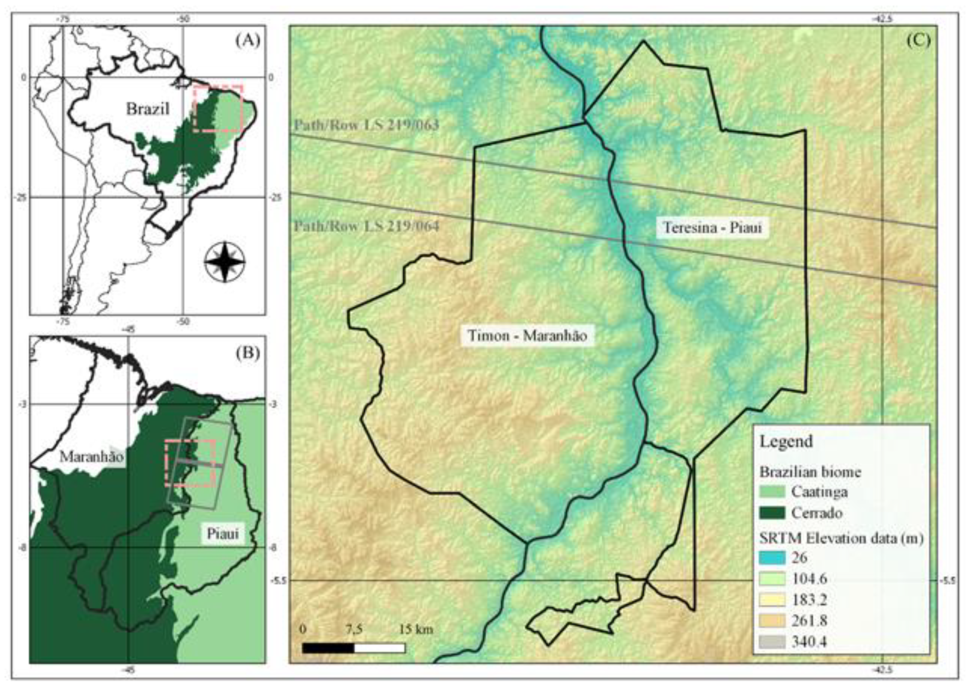
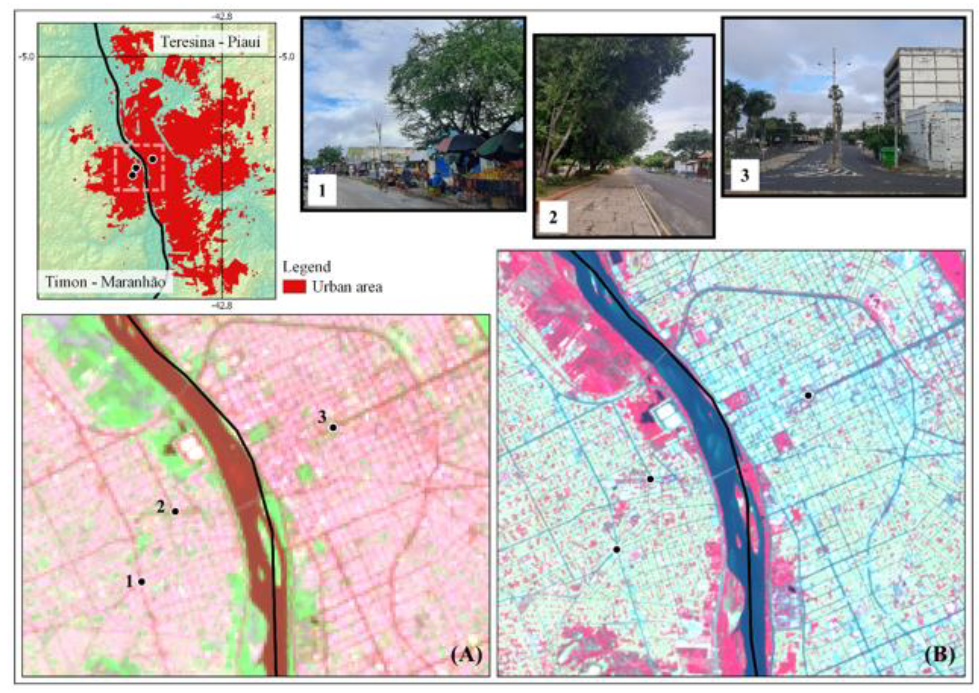
2.1. Study Area

The two adjacent cites of Teresina, in the Brazilian state of Piauí (PI), and Timon, in Maranhão (MA), have been growing at an accelerated rate over the last few decades. Teresina-Timon conurbation (TTC) area is one of the three Brazilian Integrated Economic Development Regions (IEDR) of bi-state urban areas and more than one federative unit. The Brazilian IEDR’s are similar to metropolitan areas, though, the individual cities at the IEDR’s are under distinct political-institutional arrangements. Teresina and Timon are connected by three bridges, across the 300 m wet border of the Parnaíba River. These cities share flows of commodities, capital, and inhabitants every day, and their urban dynamics over the years is an interdependent system.
The TTC urban agglomeration is located in the semiarid region of the northeast of Brazil, placed among the Cerrado and Caatinga biomes (Figure 1). This ecotone zone comprises natural vegetation characterized by a mix of semi-humid forest and savannas, with most of them degraded by mosaics of agriculture or pasture. Teresina-Timon conurbation area has a semiarid climate with recurrent droughts, which historically had motivated major waves of rural-urban migration [12,27]. The total population estimated in 2019 was equal to one million inhabitants, with averaged population densities varying from 89.18 persons per km2 in Timon municipality to 584.94 persons per km2 in Teresina (Table 1). In terms of the total population, Timon is larger than the second most populated city in the state of Piauí, after Teresina. Both cities have most of the urban population concentrated into their continuous fabric, circumcised by an expressive rural area.
Each one of these two cities has implemented different urban strategies over the past several years, although both cities have been following the main dimensions of the 2001 City Statute, the legal framework governing urban development and management in Brazil [28]. Teresina, as the capital of Piauí, and a major center for commerce, industry, and services, concentrates the majority of efforts on urban municipal legislation, regarding the delimitation of urban districts and guidelines for urban occupation, recently increasing its attention to environmental sustainability. The building areas in Teresina are much more concentrated than in Timon, and the arborization in the streets in the Teresina downtown are, as a result, also less evident (Figure 2) [27,29,30]. However, despite the interdependency among these two cities, there are still little efforts to understand the TTC urban dynamics as a unit. We lack information on the timing and magnitude of their changes, and although the Human Development Index (HDI) among these two cities is relatively close (Table 1: 0.751 in Teresina, and 0.649 in Timon), the percentage of wastewater sanitation network, for example, varies mostly (Table 1: 61.6% in Teresina, and 38.0% in Timon).

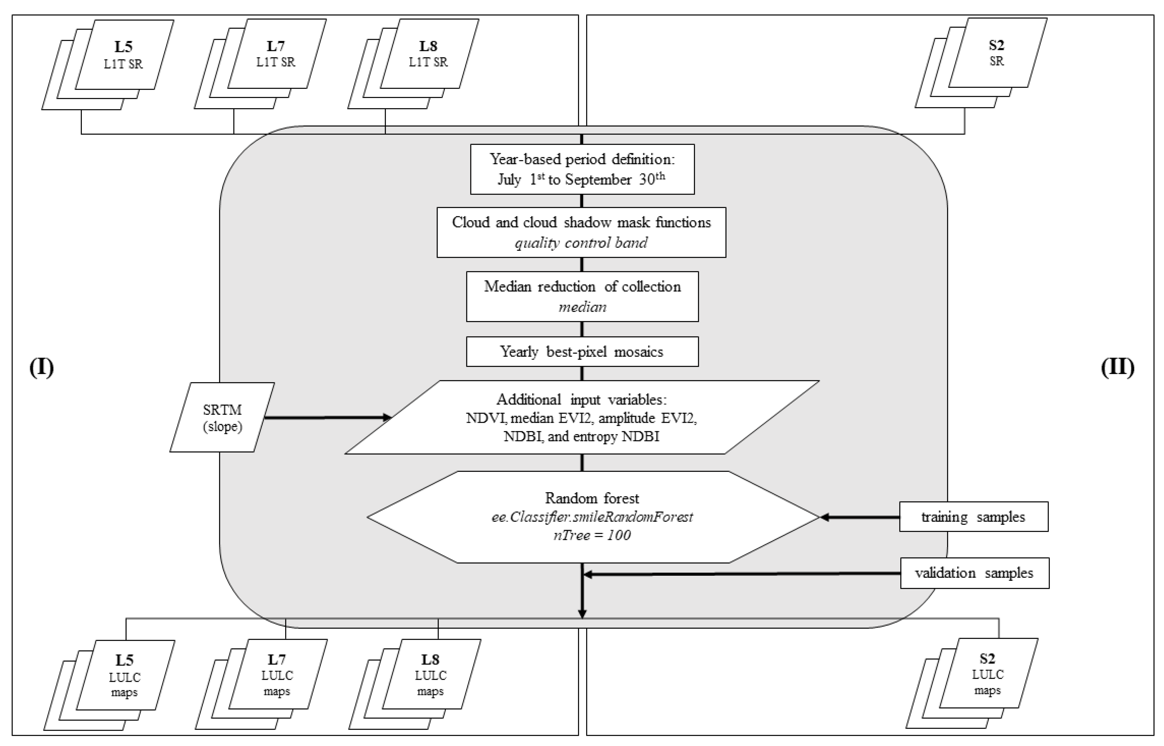
2.2. Classification Approach

Figure 3 presents the proposed framework to generate urban land maps. Our framework is virtually the same for our two major procedures: (I) classification of yearly mosaics of Landsat (LS) collection from 1985 to 2018; and (II) classification of the yearly mosaic of Sentinel-2 (S2) collection in 2019. Regarding the territorial coverage, we classified the entire two municipalities in (I); and the two adjacent urban lands in (II). In addition to the selection of different datasets, we also made adaptations on each procedure regarding the thematic land use and land cover (LULC) classes and the sample points used (Table 2). Our workflow procedure was based in Rosa [31] and Alencar et al. [32].

2.2.1. Yearly Landsat and Sentinel-2 Mosaics

We processed Thematic Mapper (TM) Landsat-5 (L5), Enhanced Thematic Mapper Plus (ETM+) Landsat-7 (L7), Operational Land Imager (OLI) Landsat-8 (L8), and MultiSpectral Instrument (MSI) Sentinel-2 (S2) imagery, accessed via Google Earth Engine (GEE) platform (https://earthengine.google.com (15 February 2021)). For Landsat (LS) mosaics, we used atmospherically corrected surface reflectance (SR) data (Collection 1 Tier 1 surface reflectance), at 30 m spatial resolution, and with five visible and near-infrared (VNIR) bands plus two short-wave infrared (SWIR) bands, processed to orthorectified reference [33]. For Sentinel-2 (S2) mosaic, we used surface reflectance (Level-2A) data [34,35]. For this last collection, we selected all four 10 m, spatial resolution bands, from visible and near-infrared spectral lengths and one short-wave infrared band at 20 m spatial resolution (Table 3 and Table 4).
We produced yearly best-pixel mosaics by merging pixels of distinct images collected from 1st July to 30th September [32], which covers the dry season. The date filtering returned a range of five to ten LS scenes for each path/row (219/063 and 219/064) in each year. We applied cloud and cloud shadow mask functions with a quality control band for each image, which returned pixels with minimum cloud coverage and better atmospheric conditions (Figure 3).
For each band, we used the GEE median function in each selected pixel-location into the period window. The resulting value was allocated for the final respective pixel-location in the annual mosaic. The median value is aimed at data dimensionality reduction and eliminating pixels corrupted by noise caused by clouds or cloud shadows not removed in the initial mask. Table 3 shows the years considered for filtering each data collection.

2.2.2. Landsat and Sentinel-2 Data Processing

Additional input variables were included in the procedure workflow, as shown in Figure 3 and Table 4. From the Landsat and Sentinel-2 datasets, we added values from the: normalized difference vegetation index (NDVI), the median of enhanced vegetation index 2 (median EVI2) [36], range of variation of EVI2 relative to the difference between the minimum and maximum values (amplitude EVI2), normalized difference built-up index (NDBI), and spatial texture computed by the entropy GEE function for NDBI values using a 5-pixel kernel centered (entropy NDBI). Furthermore, we added the slope value from the shuttle radar topography mission (SRTM). We resampled and regularized the range validity of values before inputting these new bands.
Rosa [31] and Alencar et al. [32] have shown that the addition of variables from remote sensing indexes and topographic data has contributed to the increment of the overall accuracy of classification results. For example, the amplitude EVI2 allows to better differentiate targets that remain stable throughout the year (buildings, roads, or industrial areas) from targets that vary during the year (shadows, vegetation, agriculture, or water). The textured band (entropy NDBI) allows a differentiation by the surrounding pixels, adding context information, and it helped to classify more homogeneous regions, reflecting a good generalization that is expected for classifications of urban areas.
For the classification processing, we selected the optimal parameters for the random forest (RF) algorithm from the literature (Figure 3) [37], expecting to get the highest overall classification accuracy possible. Several studies have used the number of trees equal to 100, and the number of variables in each split equal to the square root of the number of total variables [31,32,38].
Our training and validation sample data was collected based on the remote sensing visual interpretation of high-resolution imagery available in Google Earth. Based on this visual interpretation, we created polygons for each thematic land use category in areas that had not changed along the years. 80% of the total sampling in each thematic class was selected randomly from these polygons and used for training the RF algorithm, and 20% of the sample data was used for validation, considering the values described in Table 2. To assess the accuracy of classification, we used the two most popular metrics in the literature: overall accuracy (OA) and Kappa coefficient (KC), derived from the confusion matrix of the random sampling. The OA and KC coefficients were obtained for each year.

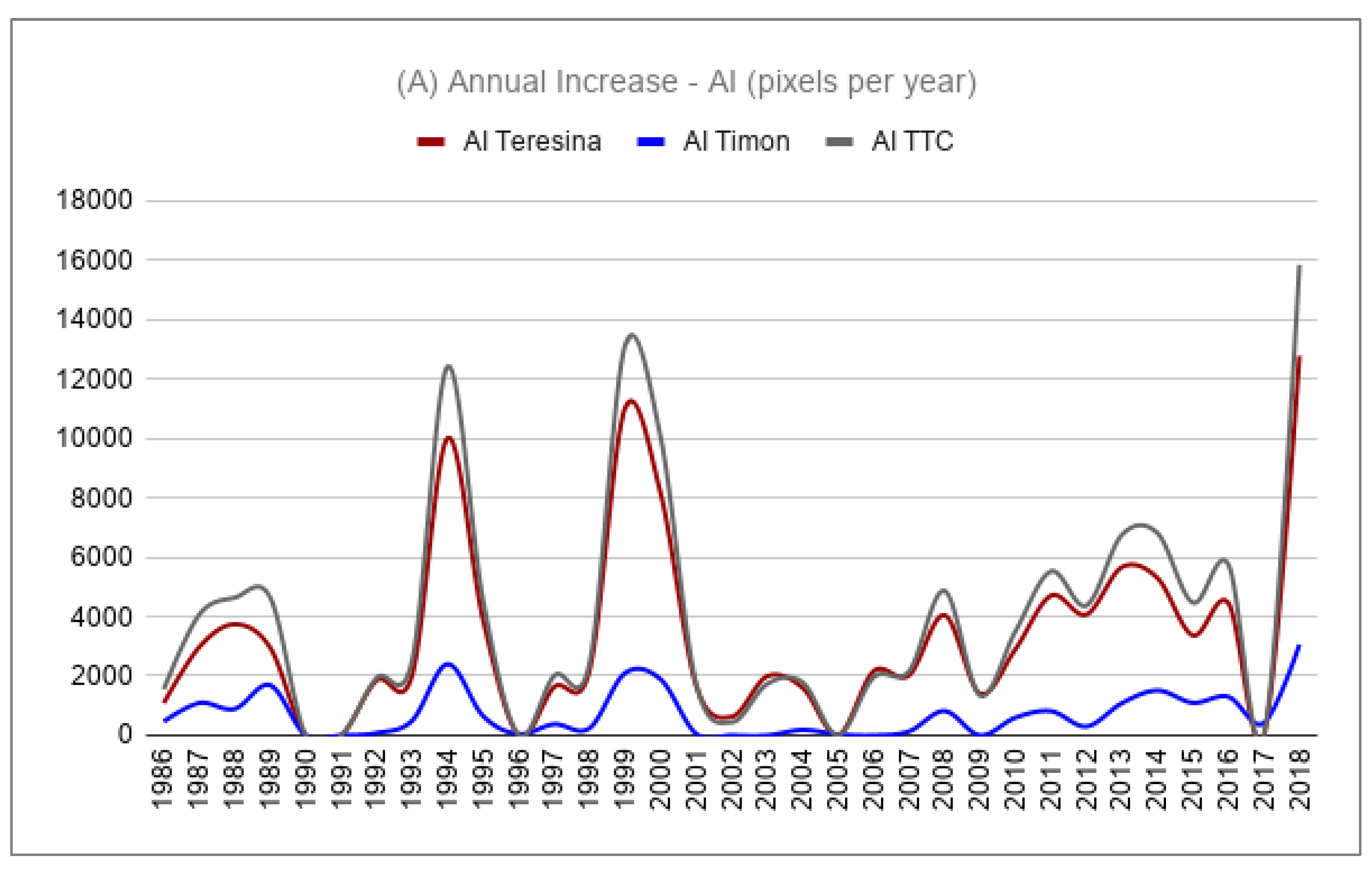
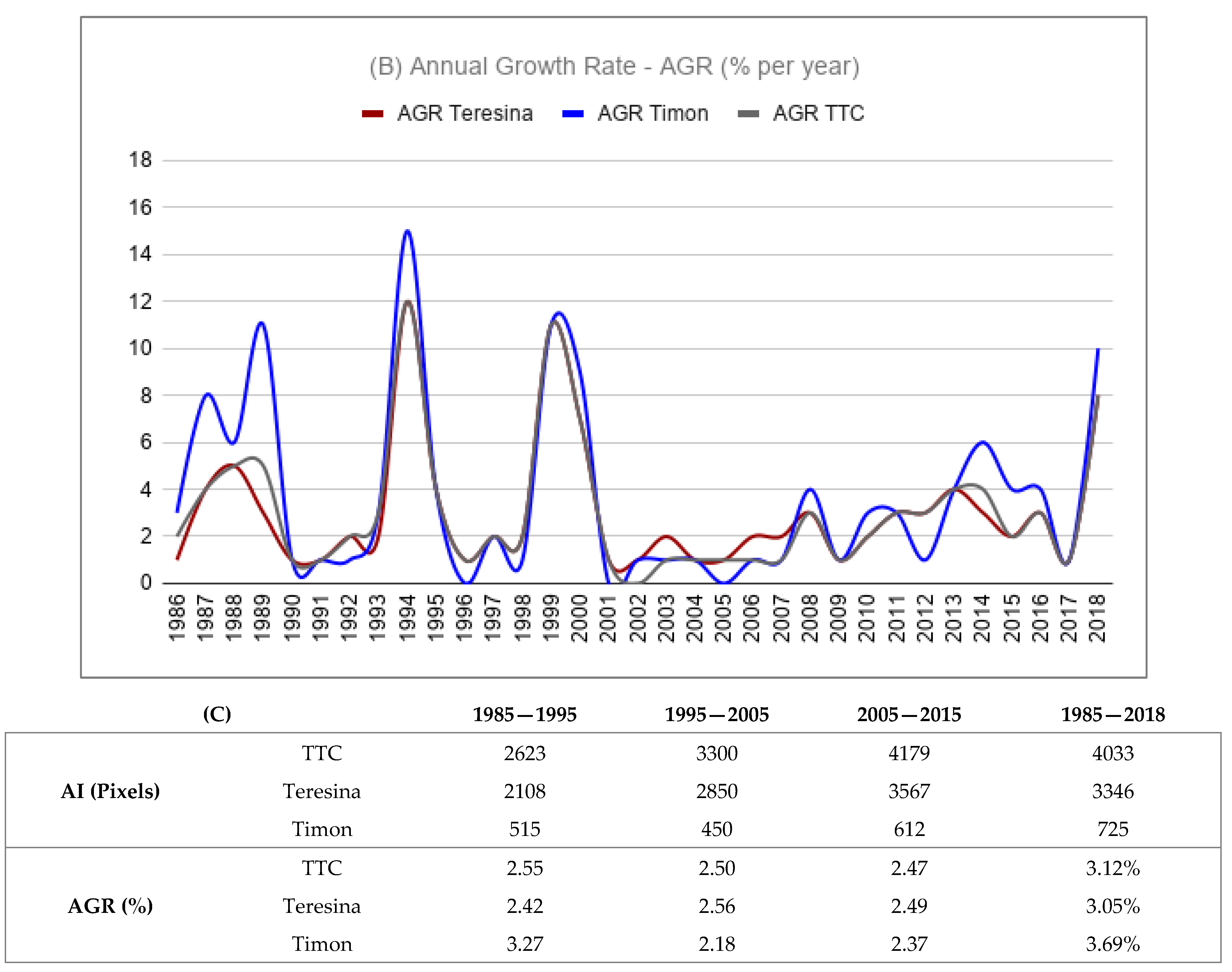
2.3. Urban Dynamics Metrics
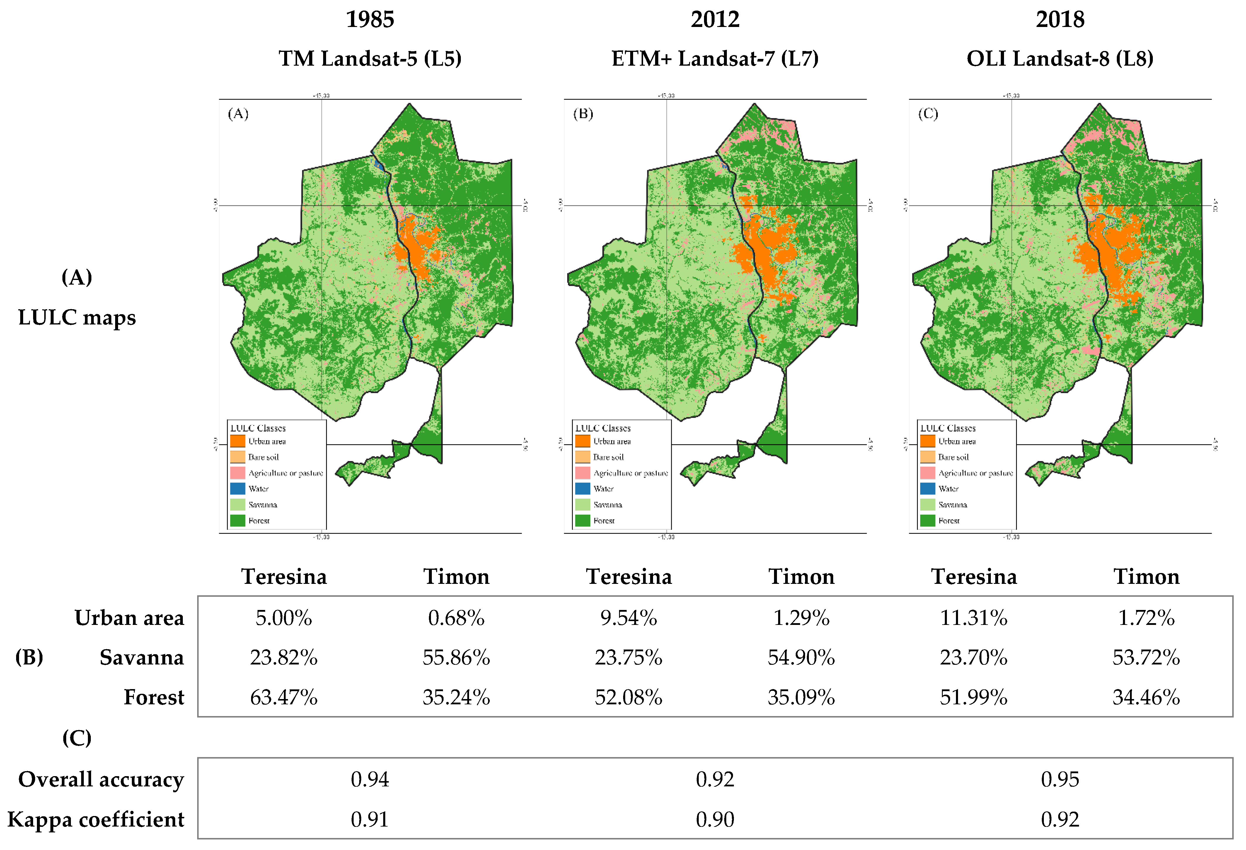
As suggested by Espindola et al. [12] and Wu et al. [39], we calculated two indexes to quantify the magnitude of urban expansion: the annual increase (AI) and the normalized annual growth rate (AGR). AI (pixels per year) and AGR (%) is the annual growth extent and the annual growth rate of the urban class, respectively. P e n d and P s t a r t are the numbers of pixels labeled as urban at the end and start periods, respectively, and d is the time interval in years.
A I = P e n d P s t a r t d
A G R = 100 % × [ ( P e n d P s t a r t ) 1 d 1 ]

3. Results

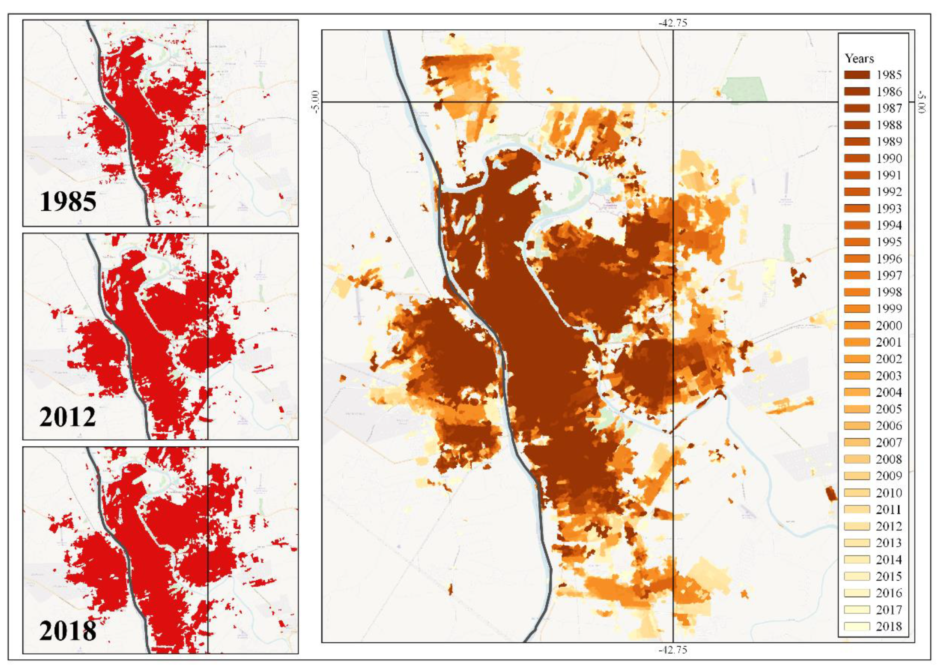
3.1. Spatial Dynamic of Urban Sprawl

The TTC area experienced notable urban expansion between 1985 and 2018. To systematically evaluate the spatial dynamics of urban sprawl over these last four decades, we present the urban land maps generated by the processing of the Landsat historical dataset. Figure 4 shows LULC maps for one selected date (1985, 2012, and 2018), and each one of the sensors used: TM (L5), ETM+ (L7), and OLI (L8), respectively. Even considering that in Figure 4 the time interval is not constant, we found it relevant to demonstrate the consistency of the LULC classification among these sensors and across the years. We see that the proportion of the urban area has increased in both municipalities, ranging from 5.00% (1985) to 11.31% (2018) in Teresina; and 0.68% (1985) to 1.72% (2018) in Timon. Teresina expanded from 70.34 km2 to 159.02 km2 from 1985 to 2018. Timon expanded from 12.20 km2 to 30.68 km2 in the same period.
Our results also demonstrate that the increment of the urban area was based on the replacement of the natural vegetation (Savanna and Forest), which has decreased considerably since 1985. Between 1985 and 2018, 161.31 km2 of Forest and 39.75 km2 of Savanna were lost. In Teresina and Timon municipalities, the predominant savanna vegetation is characterized by tree-shrub stratum, with a canopy cover of around 60%, and an averaged plant biomass and carbon stocks of 39.9 t C/ha [40]. This vegetation type differs from the forest canopy, characterized by more dense vegetation with relatively large trees, which correspond to carbon stocks of 68.6 t C/ha [40,41,42]. As an outcome, urban sprawl directly impacted the carbon and water cycles in the TTC area.
To further understand the annual patterns of urban sprawl (US) in Teresina, Timon, and in the TTC area as a unit, we show in Figure 5 the annual and continuous movement of expansion of their urban land, presenting the urban land coverage for 1985 (L5), 2012 (L7), and 2018 (L8), and each annual urban land map combined. Here, all classification results showed high overall accuracies (OA) and Kappa coefficients (KC), ranging from 90% to 95%. The combined LULC map annually demonstrates that the urban land continued to increase and expand to suburban areas. Besides, over these 33 years, Teresina and Timon have undergone rapid processes of land consumption in almost every direction from the original urban core. Our results demonstrate the feature and the trends of the urban landscape in the TTC area, as these two cities presented a monotonic increasing trajectory. In Figure 6, we analyze the main directions of the sprawling in the TTC area in more detail. Although we have a significant increase in all trends, the expansion movement to the south (S) and east (E) directions was prominent. The center of these directions is the point labeled as 3 in Figure 2.
Moreover, from Figure 7A–C, we can draw that, although the increase was constant in the TTC area, the speed of growth varied over the years. We present the magnitude of urban sprawl revealed by the annual increase (AI, in pixels) metric and normalized annual urban growth rate (AGR, %) for Teresina, Timon, and the TTC area as a unit. As the proportion of the urban area of Teresina is higher in the TTC area, the pattern of the AI in the graph (Figure 7A) is similar to the pattern presented for Teresina. In 2018, 84% of the urban land of the TTC area was in Teresina, and 16% in Timon. Then, the most massive AI occurred during the 2017–2018 period for all three areas, followed by 1998–1999 and 1993–1994. Furthermore, Figure 7A shows a positive increasing trend in the 2006–2016 decade.
After removing the effect of the city size, the TTC area, Teresina and Timon had an average AGR of 3.12%, 3.05%, and 3.69% (2018–1985), ranging from 0.30% to 12.31%, 0.51% to 11.74%, and 0.17% to 15.38% in 2018–1985 period, respectively (Figure 7B). From Figure 7C, we note that during the three decades selected, the AGR’s were almost constant across the two cities and in the conurbation area. These numbers are similar in magnitude to the ones found by Wu et al. [39] in Asian cities, such as Beijing, which had an average AGR of 3.70% in the 1980–2010 period. In another study conducted by Fu et al. [43], the annual expansion rate in another cluster of cities in China reported was between 4% and 10% during the 2000–2010 period.

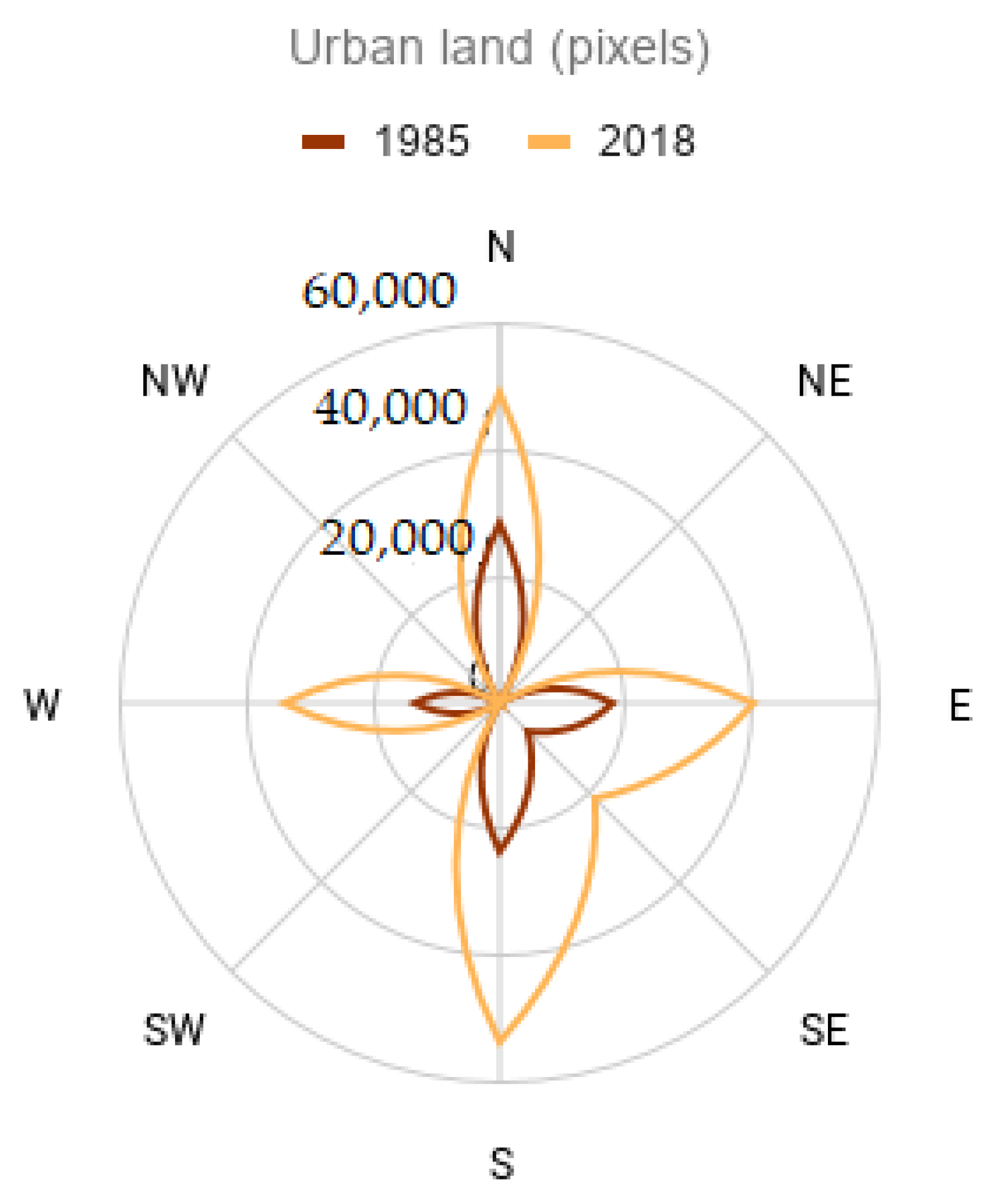
3.2. Characterization of the Urban Fabric

In Figure 8, we illustrate the 2019 LULC classification generated from the Sentinel-2 dataset. For this result, we got an OA and KC of 0.94 and 0.91, respectively. To characterize the urban fabric (UF) in the TTC area, we present the proportion of the LULC classes directly associated with intra-urban characteristics: Residential—Ceramic roofs, Residential—Other roofs, and Impervious surfaces. In the TTC area, 28.02% of the urban land was covered by ceramic roof tiles, and 11.97% by other roofs, including roofs of concrete, metallic, or asbestos. Usually, red ceramic roof tiles are associated with households, and our results show a predominance of this material with a high built-up density across Teresina (30.84%) and Timon (21.38%). On the other hand, other types of roofs are also frequent, and in this area, they are mostly associated with commercial buildings or apartments. This coverage shows a considerable difference among Teresina (15.42%) and Timon (3.85%). Indeed, part of the recent urban development of Teresina was based on vertical growth, especially in its high-income district.
In the literature, impervious surface cover is usually used as an indicator of the built-up urban land density [44]. We defined impervious surfaces as the surfaces that water cannot infiltrate. They are usually made up of anthropogenic materials, e.g., streets and roads, rooftops, parking lots, and outdoor facilities [45]. Although roof tiles may also be included in this category, we differentiate roofs in other thematic classes, aiming to distinguish places without population settlement. Even showing a similar proportion of the impervious surface in Teresina (6.45%) and Timon (3.83), the visual interpretation of our results (Figure 8B,C) demonstrates that in Timon, besides being less recurrent, this land use category is arranged with natural vegetation class. This category also corresponds to 5.67% of the total urban land in the TTC area.
The impervious surface category is relevant when associated with the urban land surface temperature. Impervious surface areas are reported to yield a temperature of around 10 degrees higher when compared with forest coverage [46]. Then, mapping this category is important for urban planning and environmental and resources management. As a result, the pattern of the land use found in Timon may contribute to an urban design that enhances the thermal comfort of the population [47].

4. Discussion

Understanding the spatial dynamics of urban development is relevant in conurbation cities under distinct political-institutional arrangements, as in the case of the Teresina-Timon area. Most remote sensing datasets are currently freely available, giving us a vast panorama of how twins cities evolved and allowing more effective urban planning. Additionally, cloud computing platforms are revolutionizing the ways we deal with image processing features. However, frameworks that integrate freely available remote sensing data into cloud computing platforms designed for urban land monitoring are still scarce. Our results showed the robustness of Landsat and Sentinel-2 imagery for urban planning and management. The use of Landsat historical imagery is well documented in the literature for monitoring urban sprawl [48,49,50,51]. On the other hand, Sentinel-2 satellites are still being evaluated [52,53,54], and we demonstrated that the urban land classes selected for this study were well classified. The ability of Sentinel-2 imagery to distinguish different types of roofs opens new possibilities for modeling populational densities in the urban land. The landscape metrics used also promoted a deeper understanding of the environmental sustainability of TTC growth.
Besides, we showed that the urban land in the TTC area presented an underlying tendency of continuous growth. Analysis results from this study suggest that, compared with other cities in Latin America, this growth has been horizontal rather than vertical. A basic finding from this study is that the TTC area’s sprawling pattern is still more relevant than the urban fabric’s densification. During the last four decades, a large amount of vegetation removal and land consumption in the TTC area imposed a critical threat to urban sustainability, as this type of land-use change is often associated with a rapid decline in local ecosystem services. In this scenario, the opening of new spaces to urban development in Teresina and Timon cities had central environmental implications, especially knowing that the main drivers of the urban fringe sprawl are usually more related to economic and agrarian factors, rather than related to the well-being of the population. The landscape analysis provided with our results summarizes the size, shape, and spatial distribution of the urban sprawl dynamics in the TTC area, reinforcing that the observed patterns are a result of complex environmental and socio-political interactions. As a conurbation area located along rivers, thus the necessity of balancing urban development and water quality should also be stressed.
In the TTC area, urban dynamics were influenced by the diversification and growth of national and local economies and by population increase. This area presented cycles of heavy urban expansion, followed by periods of sparse growth. These cycles were directly related to the importance of the federal government’s role in financing urban infrastructure. In our region, the federal grants typically followed the form of political and economic constraints.
During the 1990s, the population grew at a breakneck pace, accompanying a movement that was reported in other medium-sized cities in Brazil and Latin America [55,56,57,58,59]. After the 1990s, the TTC area sprawl was partially motivated by federal government programs that implemented national housing plans aimed to eradicate the large housing deficit in the country and focusing on low-income families.
After the 2008 economic crisis, massive investments in infrastructure displaced the population to peripheral zones without adequate urban planning, which reflected in alteration in land use and land cover (LULC), followed by environmental impacts and public health issues caused by thermal discomfort, particularly in semiarid regions. The implementation of the national housing policy in TTC contributed to the current shape of the urban land, as most of the housing settlements were in peripherical zones of Teresina and Timon. Nevertheless, the investments in urban infrastructure were never compatible with the amount of the population relocated to the new peripheral areas.
Despite empirical works that address the sprawl of Latin America medium-cities have been scarcer, commonly emphasizing only the major metropolitan areas such as São Paulo and Rio de Janeiro in Brazil, our results corroborate with Inostroza et al. [60]. Our findings show that, as a typical urban area of Latin America, TTC expressed spatial dynamics characterized by high rates of land consumption and fragmentation degrees. The TTC area manifested the same pattern of the radial growth of other Latin American cities, characterized by a low-density peripherical expansion with a lack of infrastructure, motivated by poorly regulated land use [12,61,62,63,64]. Usually, this overall tendency of sprawling growth also contributes to the reduction of residential activities in well-serviced central areas, willing to the socio-spatial segregation [65,66].

5. Conclusions

Urbanization processes are one of the major drivers affecting ecosystem functioning and services locally. In semiarid environments, urban expansion contributes to the recurrence of extreme climate events that may further impact the landscape. This study aimed to improve the understanding of urbanization processes in one conurbation area in Latin America, using cloud computing platforms and free remote sensing data. Currently, the Landsat historical dataset is the most used source to track continuous regional land-use changes back to the 1980s. However, Sentinel-2 is arising as an alternative for more detailed analysis. The high-performance of the GEE computing platform makes the manipulation of a large amount of remote sensing data more user-friendly and suitable for urban assessments and management.
Then, we proposed a semi-automatic framework to map urban land in the TTC area. The produces maps resulting in spatially explicit inventories of the urban extents and conditions. The results demonstrated that the urban agglomeration in the TTC area experienced accelerated growth from 1985 to 2019. Despite our promising results, it is still necessary to incorporate these approaches into the mainframe of urban governance that accommodates each city’s political-institutional arrangement. The joint governance of Teresian and Timon based on the use of the proposed framework would allow a more dynamic urban management by the creation of integrated urban public policies. As a future investigation, we suggest additional studies on the new dynamics of medium-sized cities in the context of urban sprawl and planning policies. We need to investigate deeper the main drivers of urban development in Latin America in contrast with distinct local, national, and international panoramas.

Author Contributions

E.C. analyzed the data and performed the experiments and computed the remote sensing analysis. W.L. and G.E. supervised the conception and design of the analysis; and worked on the final manuscript. All authors developed and discussed the manuscript together and finally wrote the paper. All authors have read and agreed to the published version of the manuscript.

Funding

UFPI and IFPI partially funded this research paper.

Acknowledgments

The authors would like to thank UFPI, IFPI for supporting this research.

Conflicts of Interest

The authors declare no conflict of interest. The funder had no role in the design of the study, in the collection, analysis, or interpretation; in the writing of the manuscript; or in the decision to publish the results.

References

  1. Moroke, T.; Schoeman, C.; Schoeman, I. Developing a neighbourhood sustainability assessment model: An approach to sustainable urban development. Sustain. Cities Soc. 2019, 48, 101433. [Google Scholar] [CrossRef]
  2. Ioppolo, G.; Cucurachi, S.; Salomone, R.; Shi, L.; Yigitcanlar, T. Integrating strategic environmental assessment and material flow accounting: A novel approach for moving towards sustainable urban futures. Int. J. Life Cycle Assess 2019, 24, 1269–1284. [Google Scholar] [CrossRef]
  3. Rovai, M.; Zetti, I.; Lucchesi, F.; Rossi, M.; Andreoli, M. Peri-urban Open Spaces and Sustainable Urban Development Between Value and Consumption. In Values and Functions for Future Cities; Springer: Berlin/Heidelberg, Germany, 2020; pp. 249–265. [Google Scholar]
  4. Friis, C.; Nielsen, J.Ø. Global Land-Use Change through a Telecoupling Lens: An Introduction. In Telecoupling; Springer: Cham, Switzerland, 2019; pp. 1–15. [Google Scholar]
  5. Obermeister, N. Local knowledge, global ambitions: IPBES and the advent of multi-scale models and scenarios. Sustain. Sci. 2019, 14, 843–856. [Google Scholar] [CrossRef]
  6. Rivera, M. Political criteria for Sustainable Development Goal (SDG) selection and the role of the urban dimension. Sustainability 2013, 5, 5034–5051. [Google Scholar] [CrossRef] [Green Version]
  7. Acuto, M.; Parnell, S.; Seto, K.C. Building a global urban science. Nat. Sustain. 2018, 1, 2–4. [Google Scholar] [CrossRef]
  8. Caprotti, F.; Cowley, R.; Datta, A.; Broto, V.C.; Gao, E.; Georgeson, L.; Herrick, C.; Odendaal, N.; Joss, S. The New Urban Agenda: Key opportunities and challenges for policy and practice. Urban Res. Pract. 2017, 10, 367–378. [Google Scholar] [CrossRef] [Green Version]
  9. Seto, K.C.; Reenberg, A.; Boone, C.G.; Fragkias, M.; Haase, D.; Langanke, T.; Marcotullio, P.; Munroe, D.K.; Olah, B.; Simon, D. Urban land teleconnections and sustainability. Proc. Natl. Acad. Sci. USA 2012, 109, 7687–7692. [Google Scholar] [CrossRef] [Green Version]
  10. Dobbs, C.; Escobedo, F.J.; Clerici, N.; de la Barrera, F.; Eleuterio, A.A.; MacGregor-Fors, I.; Reyes-Paecke, S.; Vásquez, A.; Camaño, J.D.Z.; Hernández, H.J. Urban ecosystem Services in Latin America: Mismatch between global concepts and regional realities? Urban Ecosyst. 2019, 22, 173–187. [Google Scholar] [CrossRef]
  11. Sefair, J.A.; Espinosa, M.; Behrentz, E.; Medaglia, A.L. Optimization model for urban air quality policy design: A case study in Latin America. Comput. Environ. Urban Syst. 2019, 78, 101385. [Google Scholar] [CrossRef]
  12. Espindola, G.M.; Carneiro, E.L.N.C.; Façanha, A.C. Four decades of urban sprawl and population growth in Teresina, Brazil. Appl. Geogr. 2017, 79, 73–83. [Google Scholar] [CrossRef]
  13. Almazroui, M.; Mashat, A.; Assiri, M.E.; Butt, M.J. Application of landsat data for urban growth monitoring in Jeddah. Earth Syst. Environ. 2017, 1, 1–11. [Google Scholar] [CrossRef] [Green Version]
  14. Saini, V.; Tiwari, R.K. Remote sensing based time-series analysis for monitoring urban sprawl: A case study of Chandigarh capital region. J Geom. 2019, 13, 94–97. [Google Scholar]
  15. Li, X.; Gong, P.; Liang, L. A 30-year (1984–2013) record of annual urban dynamics of Beijing City derived from Landsat data. Remote Sens. Environ. 2015, 166, 78–90. [Google Scholar] [CrossRef]
  16. Lu, Y.; Coops, N.C.; Hermosilla, T. Estimating urban vegetation fraction across 25 cities in pan-Pacific using Landsat time series data. Isprs J. Photogramm. Remote Sens. 2017, 126, 11–23. [Google Scholar] [CrossRef]
  17. Song, X.-P.; Sexton, J.O.; Huang, C.; Channan, S.; Townshend, J.R. Characterizing the magnitude, timing and duration of urban growth from time series of Landsat-based estimates of impervious cover. Remote Sens. Environ. 2016, 175, 1–13. [Google Scholar] [CrossRef]
  18. Mendili, L.E.; Puissant, A.; Chougrad, M.; Sebari, I. Towards a Multi-Temporal Deep Learning Approach for Mapping Urban Fabric Using Sentinel 2 Images. Remote Sens. 2020, 12, 423. [Google Scholar] [CrossRef] [Green Version]
  19. Iannelli, G.C.; Gamba, P. Jointly exploiting Sentinel-1 and Sentinel-2 for urban mapping. In Proceedings of the IGARSS 2018-2018 IEEE International Geoscience and Remote Sensing Symposium, Valencia, Spain, 22–27 July 2018; pp. 8209–8212. [Google Scholar]
  20. Pesaresi, M.; Corbane, C.; Julea, A.; Florczyk, A.J.; Syrris, V.; Soille, P. Assessment of the added-value of Sentinel-2 for detecting built-up areas. Remote Sens. 2016, 8, 299. [Google Scholar] [CrossRef] [Green Version]
  21. Pal, M. Random forest classifier for remote sensing classification. Int. J. Remote Sens. 2005, 26, 217–222. [Google Scholar] [CrossRef]
  22. Bhat, P.A.; ul Shafiq, M.; Mir, A.A.; Ahmed, P. Urban sprawl and its impact on landuse/land cover dynamics of Dehradun City, India. Int. J. Sustain. Built Environ. 2017, 6, 513–521. [Google Scholar] [CrossRef]
  23. Teluguntla, P.; Thenkabail, P.S.; Oliphant, A.; Xiong, J.; Gumma, M.K.; Congalton, R.G.; Yadav, K.; Huete, A. A 30-m landsat-derived cropland extent product of Australia and China using random forest machine learning algorithm on Google Earth Engine cloud computing platform. ISPRS J. Photogramm. Remote Sens. 2018, 144, 325–340. [Google Scholar] [CrossRef]
  24. He, Y.; Wang, C.; Chen, F.; Jia, H.; Liang, D.; Yang, A. Feature Comparison and Optimization for 30-M Winter Wheat Mapping Based on Landsat-8 and Sentinel-2 Data Using Random Forest Algorithm. Remote Sens. 2019, 11, 535. [Google Scholar] [CrossRef] [Green Version]
  25. Castriota, R.; Tonucci, J. Extended urbanization in and from Brazil. Environ. Plan. D Soc. Space 2018, 36, 512–528. [Google Scholar] [CrossRef]
  26. Chauvin, J.P.; Glaeser, E.; Ma, Y.; Tobio, K. What is different about urbanization in rich and poor countries? Cities in Brazil, China, India and the United States. J. Urban Econ. 2017, 98, 17–49. [Google Scholar] [CrossRef] [Green Version]
  27. Nogueira, L.L.F.; Espindola, G.M.; Carneiro, E.L.N.C. Análise da ocupação urbana na zona Centro-Norte de Teresina: Considerações sobre a região do Encontro dos Rios. Rev. Equador 2016, 5, 25–42. [Google Scholar]
  28. Gonzalez, E.L.; Chinelli, C.K.; Azevedo Guedes, A.L.; Vazquez, E.G.; Hammad, A.W.; Haddad, A.N.; Pereira Soares, C.A. Smart and sustainable cities: The main guidelines of City Statute for increasing the intelligence of Brazilian cities. Sustainability 2020, 12, 1025. [Google Scholar]
  29. De Freitas Rocha, A.T.; Mira de Espindola, G.; Araujo Soares, M.R.; de Ribamar de Sousa Rocha, J.; Nery Costa, C.H. Visceral leishmaniasis and vulnerability conditions in an endemic urban area of Northeastern Brazil. Trans. R. Soc. Trop. Med. Hyg. 2018, 112, 317–325. [Google Scholar] [CrossRef] [PubMed]
  30. Barbosa Júnior, P.A.; Espindola, G.M.; Carneiro, E.L.N.C. Cartografias do Piauí: Relacionando infraestrutura e desenvolvimento social. Rev. Geogr. Acad. 2016, 10, 56–68. [Google Scholar]
  31. Rosa, M.R. Classificação do Padrão de Ocupação Urbana de São Paulo Utilizando Aprendizagem de Máquina e Sentinel 2. Rev. Dep. Geogr. 2018, 15–21. [Google Scholar] [CrossRef]
  32. Alencar, A.; Shimbo, J.Z.; Lenti, F.; Balzani Marques, C.; Zimbres, B.; Rosa, M.; Arruda, V.; Castro, I.; Fernandes Márcico Ribeiro, J.P.; Varela, V. Mapping Three Decades of Changes in the Brazilian Savanna Native Vegetation Using Landsat Data Processed in the Google Earth Engine Platform. Remote Sens. 2020, 12, 924. [Google Scholar] [CrossRef] [Green Version]
  33. Li, S.; Wang, W.; Ganguly, S.; Nemani, R.R. Radiometric Characteristics of the Landsat Collection 1 Dataset. Adv. Remote Sens. 2018, 7, 203–217. [Google Scholar] [CrossRef] [Green Version]
  34. Drusch, M.; Del Bello, U.; Carlier, S.; Colin, O.; Fernandez, V.; Gascon, F.; Hoersch, B.; Isola, C.; Laberinti, P.; Martimort, P. Sentinel-2: ESA’s optical high-resolution mission for GMES operational services. Remote Sens. Environ. 2012, 120, 25–36. [Google Scholar] [CrossRef]
  35. Li, S.; Ganguly, S.; Dungan, J.L.; Wang, W.; Nemani, R.R. Sentinel-2 MSI radiometric characterization and cross-calibration with Landsat-8 OLI. Adv. Remote Sens. 2017, 6, 147. [Google Scholar] [CrossRef] [Green Version]
  36. Jiang, Z.; Huete, A.R.; Didan, K.; Miura, T. Development of a two-band enhanced vegetation index without a blue band. Remote Sens. Environ. 2008, 112, 3833–3845. [Google Scholar] [CrossRef]
  37. Breiman, L. Random forests. Mach. Learn. 2001, 45, 5–32. [Google Scholar] [CrossRef] [Green Version]
  38. Thanh Noi, P.; Kappas, M. Comparison of random forest, k-nearest neighbor, and support vector machine classifiers for land cover classification using Sentinel-2 imagery. Sensors 2018, 18, 18. [Google Scholar] [CrossRef] [PubMed] [Green Version]
  39. Wu, W.; Zhao, S.; Zhu, C.; Jiang, J. A comparative study of urban expansion in Beijing, Tianjin and Shijiazhuang over the past three decades. Landsc. Urban Plan. 2015, 134, 93–106. [Google Scholar] [CrossRef]
  40. Ribeiro, S.C.; Fehrmann, L.; Soares, C.P.B.; Jacovine, L.A.G.; Kleinn, C.; de Oliveira Gaspar, R. Above-and belowground biomass in a Brazilian Cerrado. For. Ecol. Manag. 2011, 262, 491–499. [Google Scholar] [CrossRef]
  41. Bonini, I.; Marimon-Junior, B.H.; Matricardi, E.; Phillips, O.; Petter, F.; Oliveira, B.; Marimon, B.S. Collapse of ecosystem carbon stocks due to forest conversion to soybean plantations at the Amazon-Cerrado transition. For. Ecol. Manag. 2018, 414, 64–73. [Google Scholar] [CrossRef]
  42. Batlle-Bayer, L.; Batjes, N.H.; Bindraban, P.S. Changes in organic carbon stocks upon land use conversion in the Brazilian Cerrado: A review. Agric. Ecosyst. Environ. 2010, 137, 47–58. [Google Scholar] [CrossRef]
  43. Fu, Y.; Li, J.; Weng, Q.; Zheng, Q.; Li, L.; Dai, S.; Guo, B. Characterizing the spatial pattern of annual urban growth by using time series Landsat imagery. Sci. Total Environ. 2019, 666, 274–284. [Google Scholar] [CrossRef]
  44. Slonecker, E.T.; Jennings, D.B.; Garofalo, D. Remote sensing of impervious surfaces: A review. Remote Sens. Rev. 2001, 20, 227–255. [Google Scholar] [CrossRef]
  45. Weng, Q. Remote sensing of impervious surfaces in the urban areas: Requirements, methods, and trends. Remote Sens. Environ. 2012, 117, 34–49. [Google Scholar] [CrossRef]
  46. Lu, D.; Weng, Q. Use of impervious surface in urban land-use classification. Remote Sens. Environ. 2006, 102, 146–160. [Google Scholar] [CrossRef]
  47. Correia Filho, W.L.F.; de Barros Santiago, D.; de Oliveira-Júnior, J.F.; da Silva Junior, C.A. Impact of urban decadal advance on land use and land cover and surface temperature in the city of Maceió, Brazil. Land Use Policy 2019, 87, 104026. [Google Scholar] [CrossRef]
  48. Rahman, M.T. Detection of land use/land cover changes and urban sprawl in Al-Khobar, Saudi Arabia: An analysis of multi-temporal remote sensing data. Isprs Int. J. Geo-Inf. 2016, 5, 15. [Google Scholar] [CrossRef]
  49. Lu, L.; Guo, H.; Corbane, C.; Li, Q. Urban sprawl in provincial capital cities in China: Evidence from multi-temporal urban land products using Landsat data. Sci. Bull. 2019, 64, 955–957. [Google Scholar] [CrossRef] [Green Version]
  50. Mohammady, S.; Delavar, M.R. Urban sprawl assessment and modeling using landsat images and GIS. Model. Earth Syst. Environ. 2016, 2, 155. [Google Scholar] [CrossRef]
  51. Grădinaru, S.R.; Kienast, F.; Psomas, A. Using multi-seasonal Landsat imagery for rapid identification of abandoned land in areas affected by urban sprawl. Ecol. Indic. 2019, 96, 79–86. [Google Scholar] [CrossRef]
  52. Benedetti, A.; Picchiani, M.; Del Frate, F. Sentinel-1 and sentinel-2 data fusion for urban change detection. In Proceedings of the IGARSS 2018-2018 IEEE International Geoscience and Remote Sensing Symposium, Valencia, Spain, 22–27 July 2018; pp. 1962–1965. [Google Scholar]
  53. Loret, E.; Martino, L.; Fea, M.; Sarti, F. Enhanced urban sprawl monitoring over the Entire District of Rome through joint analysis of ALOS AVNIR-2 and SENTINEL-2A data. Adv. Remote Sens. 2017, 6, 76. [Google Scholar] [CrossRef] [Green Version]
  54. Rahar, P.S.; Pal, M. Comparison of Various Indices to Differentiate Built-up and Bare Soil with Sentinel 2 Data. In Applications of Geomatics in Civil Engineering; Springer: Berlin/Heidelberg, Germany, 2020; pp. 501–509. [Google Scholar]
  55. Bolay, J.-C.; Rabinovich, A. Intermediate cities in Latin America risk and opportunities of coherent urban development. Cities 2004, 21, 407–421. [Google Scholar] [CrossRef] [Green Version]
  56. Henríquez, C.; Azócar, G.; Romero, H. Monitoring and modeling the urban growth of two mid-sized Chilean cities. Habitat Int. 2006, 30, 945–964. [Google Scholar] [CrossRef]
  57. Da Mata, D.; Deichmann, U.; Henderson, V.J.; Lall, S.V.; Wang, H.G. Examining the Growth Patterns of Brazilian Cities; The World Bank: Washington, DC, USA, 2005. [Google Scholar]
  58. Ferguson, B.W. Inducing local growth: Two intermediate-sized cities in the state of Parana, Brazil. Third World Plan. Rev. 1992, 14, 245. [Google Scholar] [CrossRef]
  59. Sridhar, K.S.; Wan, G. Firm location choice in cities: Evidence from China, India, and Brazil. China Econ. Rev. 2010, 21, 113–122. [Google Scholar] [CrossRef] [Green Version]
  60. Inostroza, L.; Baur, R.; Csaplovics, E. Urban sprawl and fragmentation in Latin America: A dynamic quantification and characterization of spatial patterns. J. Environ. Manag. 2013, 115, 87–97. [Google Scholar] [CrossRef] [PubMed]
  61. Barton, J.R.; Ramírez, M.I. The Role of Planning Policies in Promoting Urban Sprawl in Intermediate Cities: Evidence from Chile. Sustainability 2019, 11, 7165. [Google Scholar] [CrossRef] [Green Version]
  62. Monkkonen, P.; Comandon, A.; Escamilla, J.A.M.; Guerra, E. Urban sprawl and the growing geographic scale of segregation in Mexico, 1990–2010. Habitat Int. 2018, 73, 89–95. [Google Scholar] [CrossRef] [Green Version]
  63. Huang, J.; Lu, X.X.; Sellers, J.M. A global comparative analysis of urban form: Applying spatial metrics and remote sensing. Landsc. Urban Plan. 2007, 82, 184–197. [Google Scholar] [CrossRef]
  64. Alencar, P.G.d.; de Espindola, G.M.; da Costa Carneiro, E.L.N. Dwarf cashew crop expansion in the Brazilian semiarid region: Assessing policy alternatives in Pio IX, Piauí. Land Use Policy 2018, 79, 1–9. [Google Scholar] [CrossRef]
  65. Machado, A.L.M.; Maraschin, C. Urban segregation and socio-spatial interactions: A configurational approach. Urban Sci. 2018, 2, 55. [Google Scholar]
  66. Lopes, L.; Motte-Baumvol, B.; Thévenin, T. Urban Mobility and the Spatial Distribution of Economic Activities in Rio de Janeiro (Brazil). The European Colloquium on Theoretical and Quantitative Geography (ECTQG). 2017. Available online: https://hal.archives-ouvertes.fr/hal-01744913/ (accessed on 15 February 2021).
Figure 1. Location of the study area: (A) Cerrado and Caatinga biomes in Brazil; (B) Maranhão (MA) and Piauí (PI) Brazilian states, and the location of Landsat (LS) scenes of path/row 219/063 (north) and 219/063 (south); (C) Timon-MA and Teresina-PI municipalities, and the Shuttle Radar Topography Mission (SRTM) elevation map.
Remotesensing 13 01338 g001
Figure 2. Urban area coverage of Teresina-Timon conurbation (TTC) expansion in 2018 with the location of panoramic field photos; (A) Operational Land Imager (OLI) Landsat-8 color composition, bands 6(R)5(G)4(B), acquisition date in 07/12/2019, vegetation appears green and urban area has a magenta hue; (B) Multispectral Instrument (MSI) Sentinel-2A color composition, bands 8(R)4(G)3(B), acquisition date in 08/11/2019, vegetation appears red and urban area has a blue hue; (1 and 2) panoramic field photos of Timon; (3) panoramic field photo of Teresina.
Remotesensing 13 01338 g002
Figure 3. The workflow of the procedures with sensors: TM Landsat-5 (L5), ETM+ Landsat-7 (L7), OLI Landsat-8 (L8), and MSI Sentinel-2 (S2). For Landsat (LS) dataset: Collection 1, Tier 1, orthorectified surface reflectance (L1T SR). For Sentinel-2 dataset: surface reflectance (SR) Level-2A. Additional variables: Normalized Difference Vegetation Index (NDVI), Enhanced Vegetation Index 2 (EVI2), Normalized Difference Built-Up Index (NDBI), Shuttle Radar Topography Mission (SRTM).
Remotesensing 13 01338 g003
Figure 4. (A) TM (L5), ETM+ (L7), and OLI (L8) LULC maps from 1985, 2012, and 2018, respectively. (B) The proportion of LULC thematic classes: Urban area, Savanna, and Forest in Teresina and Timon municipalities. (C) Overall accuracy (OA) and Kappa coefficient (KC) of each LULC classification.
Remotesensing 13 01338 g004
Figure 5. Urban land classification obtained from TM (L5), ETM+ (L7), and OLI (L8) imagery from 1985, 2012, and 2018, respectively. Resultant temporal urban sprawl from 1985 to 2018 in the TTC area.
Remotesensing 13 01338 g005
Figure 6. Changes in pixels (spatial resolution of 30 m) of urban land coverage from 1985 to 2018 for each of the five sectors (N, E, SE, S, and W) in the TTC area in 1985 and 2018.
Remotesensing 13 01338 g006
Figure 7. (A) Annual increase (AI) (in pixels) for each year from 1985 to 2018 for: TTC area (grey); Teresina (red); and Timon (blue). (B) Normalized annual urban growth rate (AGR) (%) for each year from 1985 to 2018 for: TTC area (grey); Teresina (red); and Timon (blue). (C) AI and AGR computed for decades: 1985—1995, 1995—2005, 2005—2015, and the average for 1985—2018 period.
Remotesensing 13 01338 g007aRemotesensing 13 01338 g007b
Figure 8. 2019 LULC map derived from Sentinel-2 data. (A) TTC urban area. (B) Subset showing the central zone of Teresina. (C) Subset showing the central zone of Timon. The proportion of LULC thematic classes in the urban area: Residential—Ceramic roofs, Residential—Other roofs, and Impervious surface.
Remotesensing 13 01338 g008
Table 1. Socioeconomic characterization of the Teresina-Timon conurbation area.
CharacteristicsTeresinaTimon
Brazilian statePiauí (PI)Maranhão (MA)
Population estimated in 2019864,845 inhabitants169,107 inhabitants
Population surveyed in 2010814,230 inhabitants155,460 inhabitants
Urban population in 201080.54%71.15%
Population density in 2010584.94 persons per km289.18 persons per km2
Total area1391.046 km21764.612 km2
Human Development Index (HDI) in 20100.7510.649
Wastewater sanitation network61.6%38.0%
Table 2. List of the thematic LULC classes used with each remote sensing dataset—Landsat and Sentinel-2, and quantities of sample data used, respectively.
Thematic Classes for Landsat (I)Quantities of Sample Data
Urban area1463
Bare soil1484
Agriculture or pasture1249
Water1495
Savanna1495
Forest1441
Thematic Classes for Sentinel-2 (II)Quantities of Sample Data
Residential—Ceramic roofs1457
Residential—Other roofs1459
Impervious surfaces1386
Bare soil1484
Water1495
Natural vegetation (Savanna and Forest)1492
Table 3. Temporal coverage considered for Landsat (LS) and Sentinel-2 (S2) data.
Sensor/SatelliteFiltered CollectionSpatial Resolution
TM Landsat-5 (L5)1985 to 2011 30 m
ETM+ Landsat-7 (L7)201230 m
OLI Landsat-8 (L8)2013 to 201830 m
MSI Sentinel-2 (S2)201910 m
MSI Sentinel-2 (S2)201920 m (Band 11 only)
Table 4. List of predictive input variables considered to be included in the classification procedures. TM Landsat-5 (L5), ETM+ Landsat-7 (L7), OLI Landsat-8 (L8), MSI Sentinel-2 (S2), and Shuttle Radar Topography Mission (SRTM).
Input VariableMeaning/Formula
Blue bandBand 1 (L5 and L7); Band 2 (L8); Band 2 (S2)
Green bandBand 2 (L5 and L7); Band 3 (L8); Band 3 (S2)
Red bandBand 3 (L5 and L7); Band 4 (L8); Band 4 (S2)
Near-infrared (NIR) bandBand 4 (L5 and L7); Band 5 (L8); Band 8 (S2)
Short-wave infrared (SWIR1) bandBand 5 (L5 and L7); Band 6 (L8); Band 11 (S2)
Short-wave infrared (SWIR2) bandBand 7 (L5, L7, and L8)
Normalized Difference Vegetation Index (NDVI) N D V I = N I R     R e d N I R   +   R e d
Enhanced Vegetation Index 2 (EVI2) E V I 2 = 2.5 N I R     R e d N I R   +   2.4   R e d   +   1
Normalized Difference Built-Up Index (NDBI) N D B I = S W I R 1     N I R S W I R 1   +   N I R
Shuttle Radar Topography Mission (SRTM)Slope (in degrees)
Publisher’s Note: MDPI stays neutral with regard to jurisdictional claims in published maps and institutional affiliations.

