Article

Spatial Correlation between Ecosystem Services and Human Disturbances: A Case Study of the Guangdong–Hong Kong–Macao Greater Bay Area, China

1
Key Laboratory of Ocean and Marginal Sea Geology, Guangzhou Institute of Geochemistry, Chinese Academy of Sciences, Guangzhou 510640, China
2
University of Chinese Academy of Sciences, Beijing 100049, China
3
School of Environment, Jinan University, Guangzhou 511443, China
4
Guangdong Academy of Social Sciences, Guangzhou 510635, China
*
Author to whom correspondence should be addressed.
Remote Sens. 2021, 13(6), 1174; https://doi.org/10.3390/rs13061174
Submission received: 9 January 2021 / Revised: 14 March 2021 / Accepted: 17 March 2021 / Published: 19 March 2021
(This article belongs to the Special Issue Human–Environment Interactions Research Using Remote Sensing)

Abstract

:
Exploring the spatial relationship between ecosystem services (ES) and human disturbance intensity (HDI) is vital for maintaining regional ecological security. This study aims to explore the spatial correlation between ES and HDI in the Guangdong–Hong Kong–Macao Greater Bay Area (GBA) and provide meaningful implications for coastal ecological planning. Multi-source remote sensing data, remote sensing software, and geographic information system provided initial data and technical support for this research. We integrated four human pressures (population, land-use, traffic, and energy) to map the HDI in the GBA for 2018. Coastal ES were comprehensively considered and spatially visualized by extracting the ES sources. The geographically weighted Pearson correlation coefficient and bivariate local Moran were used to quantitatively reflect and spatially visualize the detailed relationship between ES and HDI. Our study presents several key findings. First, the central and southern parts of the GBA are under strong HDI, dominated by a dense population and intense land utilization. Second, the kernel density of ES sources can better manifest the spatial distribution of ES objectively in comparison to the traditional model calculation. Provisioning services mainly originate from the periphery of the central cities; cultural services are highly concentrated in the heartland of the GBA; and regulating and maintenance services have high density in the outermost regions. Third, ES and HDI have a significant correlation, and the geographically weighted Pearson correlation coefficient and local indicator of spatial association cluster maps illustrate that unlike the global findings, the local correlation is spatially nonstationary as the local scale is affected by specific human activities, natural conditions, regional development, and other local factors. Four, high-capacity regions of ES provision are mainly under high HDI. Areas with high provisioning service values are mainly affected by population and traffic pressure, whereas regulating and maintenance services and cultural services are mainly dominated by high-density populations. Regulating and maintenance services are also affected by land-use pressure. We determine that human disturbance has negative spillover effects on ES, which should be the focus in regional ecological planning.

Graphical Abstract

1. Introduction

Ecosystem services (ES) are defined as the benefits people directly or indirectly obtain from ecosystems; they are classified into three categories by the Common International Classification of Ecosystem Services (CICES): provisioning, regulating, and maintenance, and cultural services [1]. These services are a necessary basis for socioeconomic development; ES abundance is also a resilience descriptor for ecological security [2]. Intensified human disturbance and the tight-coupled human–environment system have dramatic impacts on the quality and quantity of ES [3,4,5,6,7]. Coastal areas are economically important and provide abundant ES. However, coastal regions are ecologically fragile and sensitive to environmental change [8]. The vulnerability of coastal ecosystems has been increasing as a result of human perturbations that compromise the ability to provide multiple ecosystem services. Human pressures caused by natural resource exploitation, infrastructure construction, and sea reclamation can exert irreversible effects on coastal ecosystems [9,10,11]. Therefore, exploring the spatial relationship between ES and human disturbance intensity (HDI) is fundamental to making informed decisions regarding regional ecological security and alleviating the contradiction between ES supply and human demand.
The dynamic mechanism between human activities and ES has been a topic of considerable interest in studies on human–nature interaction systems. Many studies have been conducted to construct a globally standardized measure of the human footprint on natural ecosystems. Sanderson et al. (2002) mapped the intensity of human influence over the entire land surface based on remote sensing data from the early 1990s [12]. It is the most complete and with the highest resolution global dataset of accumulated human pressure on the environment. Halpern (2008) developed an ecosystem-specific and multiscale spatial model to synthesize 17 global datasets of anthropogenic drivers of ecological change for 20 marine ecosystems [13]. Venter et al. (2016) used 1 km2 resolution remote sensing data from 1993 to 2009 of infrastructure, land cover and human access to natural areas to construct a globally standardized measure of the cumulative human footprint on the terrestrial environment [14]. Tapia-Armijos et al. (2017) tailored the Human Footprint Index at the global level to evaluate the spatial and temporal patterns of human pressure in the protected areas of South Ecuador [15]. These studies indicate that human demands on natural systems are accelerating and could be undermining the stability of ecosystems, and that most regions are strongly affected by multiple artificial drivers. They also suggest that remote sensing can play a significant role in human–nature interaction research for important initial data and technical support.
The main human disturbance factors vary between spatial scales, and differ by geographical location; furthermore, global datasets and measurements often overlook information that may be unique to specific localities. Rogers et al. (2010) incorporated human-related threats obtained by remote sensing data processing with ES and biological measures to identify priorities within a developing protected area network [16]. Li (2018) used human footprint scores processed by Landsat datasets to reveal the spatial relationships between the human footprint and the environmental quality of nature reserves in Tibet [17]. Mustafa and Blaine (2020) examined the variation in habitat quality associated with HDI [18]. Although these studies attempted to explore the interaction between ES and HDI in local areas, there are still some factors that remain unexplored (like the clustering patterns between ES and HDI), especially at the local scale. Peng et al. (2017) used linear regression to estimate the linear relationship between the total ES value and three indicators of urbanization [19]. Nevertheless, linear regression and the global Moran method for correlation analysis can merely analyze the correlation quantitatively, and the correlation cannot be visualized in space [20,21].
The aforementioned studies were conducted in inland nature reserves and habitats; research on sensitive coastal areas with important ecological functions is relatively scarce. Compared with terrestrial ecosystems, coastal areas have more complex environmental conditions and ecosystem components. Existing studies have mainly estimated and mapped the value of ES [7,22,23], which seriously underestimate the actual value of ES in coastal areas. Therefore, determining ways to effectively and comprehensively identify the types and distribution characteristics of ES in coastal urban areas is of great significance for ecological planning, and ecosystem function restoration and improvement in coastal zones. Hu et al. (2019) used the hot/cool-spot mapping method to assess the patterns of ES values in the Pearl River Delta, and discussed the response mechanism of ES value to land-use/cover changes [24]. However, there have been no studies on human-nature interactions in the coastal region of south China.
This study aims to explore the spatial relationship between ES and HDI in the Guangdong–Hong Kong–Macao Greater Bay Area (GBA) in 2018 and provide foundations for mitigating environmental damage in sensitive or ecologically valuable coastal areas. The objectives of this study are to: (1) map the cumulative HDI by incorporating four types of human pressures based on multi-source remote sensing data; (2) depict the spatial pattern of ES according to the coastal ES classification system; (3) analyze the spatial correlations and clustering patterns of ES and HDI; and (4) identify the implications for coastal ecological planning.
The GBA is the fourth largest bay area in the world, and it is one of the most economically vibrant regions in China. In recent decades, large-scale land exploitation and reclamation have been carried out, which have resulted in irreversible adverse effects on the coastal ecological environment [25]. To ensure the harmonious and sustainable development of human society and environmental preservation in the GBA, it is important to explore the spatial correlation between HDI and ES. In this study, we mapped the cumulative HDI by incorporating four main types of human pressures in the GBA (population, land-use, traffic, and energy). Pressures caused by navigable waterways were included to ensure the HDI calculation reflected the specific context of coastal zones. The spatial pattern of ES was depicted according to the coastal ES classification system; the multiple types of ES provided by coastal ecosystems were fully considered. The density analysis of points of interest could reflect urban economic and population hotspots [26]. Therefore, we extracted the ES source points to visualize the spatial distribution of ES hotspots and calculated the kernel density for the division of regional ES capacity. The kernel density of ES sources surpasses the subjectivity of traditional modeling methods and manifests the spatial distribution of ES more objectively [27]. The spatial correlations and clustering patterns of ES and HDI were analyzed by applying the geographically weighted Pearson correlation coefficient and the local spatial autocorrelation, which can spatially visualize and quantitatively reflect the correlation between the two variables in the local area.

2. Materials and Methods
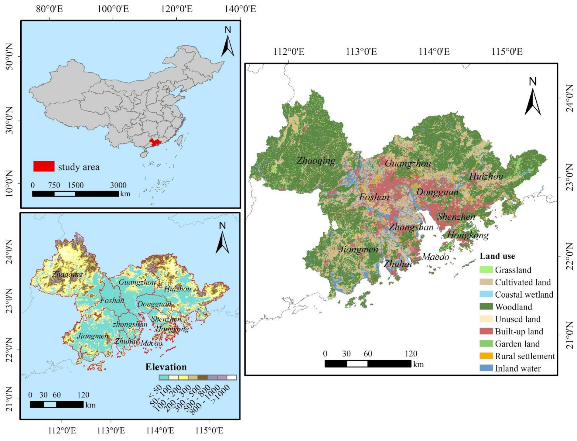
2.1. Study Area

The GBA is located in southern China (21°25′ N–24°30′ N, 111°12′ E–115°35′ E) and covers a total area of 56,000 km2 (Figure 1). It consists of the Pearl River Delta and two special administrative regions (Hong Kong, and Macao); the region plays a significant strategic role in the land-based “Silk Road Economic Belt,” and “the 21st Century Maritime Silk Road” [28]. The GBA is characterized by subtropical and tropical monsoon climates; it records an annual average precipitation ranging from 1300 mm to 2500 mm, an average temperature of 22.3 °C, and exhibits two primary seasons: a high-temperature summer with more rain, and a milder winter, with less rain. The altitude is higher in the north, and lower in the south. The mountains are mainly distributed in the northeast and northwest regions; the central and coastal zones are dominated by plains [29].

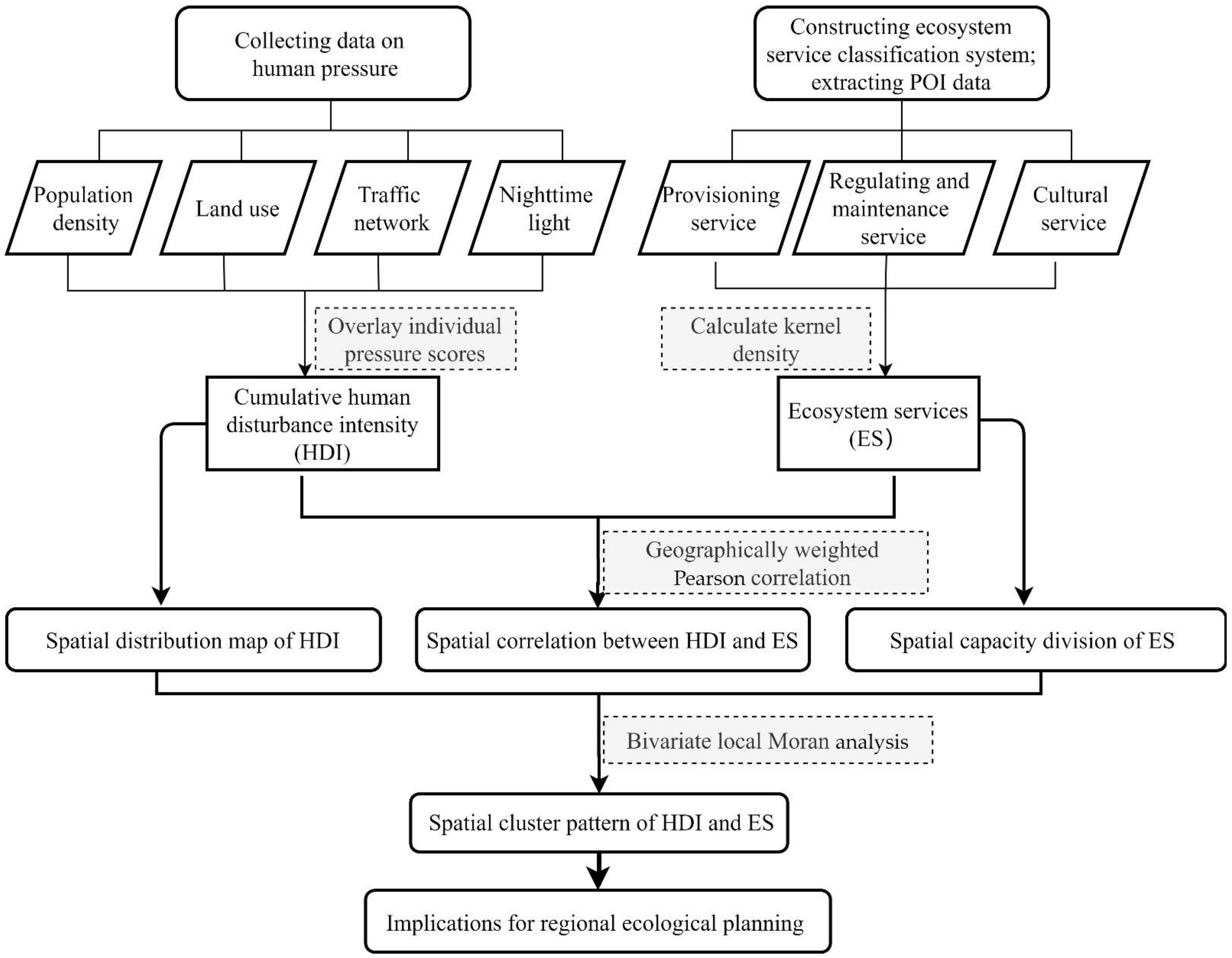
2.2. Overview of the Methodological Steps

In this study, four main types of human disturbance were identified and superposed to obtain the cumulative HDI. Three types of ES were identified based on the coastal ES classification system and were extracted via the points of interest extractor. The spatial correlations and clustering patterns of ES and HDI were analyzed using the geographically weighted Pearson correlation coefficient in R Programming language and bivariate local Moran in GeoDa software. The flow chart of the entire process is shown in Figure 2.

2.3. Human Disturbance Intensity

The human population of the GBA far exceeds that of the other three world-class bay areas (New York Bay Area, San Francisco Bay Area, and Tokyo Bay Area); in 2018, the GBA recorded a population density of 881.17 people/km2 [29,30]. Population growth has increased the burden on the local ecological environment.
A large number of reclamation projects have been conducted in coastal areas and the offshore islands of the GBA. The built-up land covers an area of 6769.17 km2, which accounts for 12.18% of the total land area of the GBA. High-intensity human activities have led to changes in land cover to varying degrees and have greatly affected the ecosystem [31,32]. We preprocessed the remote sensing images (Landsat 8 OLI/TIRS) using ENVI 5.3, including performing geometric, radiometric, atmospheric corrections, image cropping, and mosaics, and then classified the preprocessed images through support vector machine supervised classification to obtain the land-use data. We combined Google Earth data with land-use data to establish a confusion matrix to verify the accuracy of the classification results. The verification results show a Kappa coefficient >0.85, which means the interpretation accuracy meets the use requirements of medium-resolution remote sensing images.
Dense transportation networks negatively affect the integrity of the ecological landscape, aggravate landscape fragmentation, and weaken landscape connectivity [33]. In 2018, the GBA had 4300 km of highways, and the road network density was much higher than that of New York, Tokyo, London, the Yangtze River Delta, the Beijing–Tianjin–Hebei region, and other domestic and foreign city clusters [28,29,30]. In addition, the degree of connectivity of the night-time lights in the GBA is significantly higher than in other urban agglomeration.
Satellite images capture visible lights at night and indicate the degree of development of an area [34]. There is a strong correlation between power consumption intensity and night-time light disturbance [35,36].
Considering the aforementioned observation, we took the four types of human disturbance as leading contributors to cumulative HDI; the data sources are shown in Table 1. We used a 3 km × 3 km vector grid as the spatial unit for analysis to extract the mean value of multi-source data in ArcGIS. Then, the disturbance intensity scores were calculated according to the corresponding formula.

2.3.1. Disturbance Intensity of Population

We assigned a disturbance intensity score of 10 for grids with more than 1000 people/km2; this was based on the assumption that the influence of the human population approached an asymptote at 1000 people/km2 [3]. Owing to the higher population density in developed coastal areas, the asymptote was set to 1000 rather than 10 inhabitants/km2 as was used in global datasets. For pixels with population density below 1000 people/km2, the population disturbance score P D I S was determined using the calculation method as in global datasets [14].
P D I s =                   10 ,                         P d 1000   people   /   km 2     3.333 × log P d + 1 ,       P d < 1000   people   /   km 2
The value of P D I S is in the range (0, 10]; the higher the score, the stronger is the disturbance intensity.
Nor P D I S i = P D I S i min P D I s max P D I s min P D I s ,
where Pd is the population density, and where Nor P D I S i is the normalized P D I S of each grid, and ranges from 0 to 1. P D I S i is the P D I S of grid i, max P D I s is the maximum of P D I s in all grids, and min P D I s is the minimum of P D I s in all grids.

2.3.2. Disturbance Intensity of Land-Use

The areas of each land-use type in each grid were calculated using the research method developed by Brentrup et al. (2002) [40]. The calculation formula for the land-use intensity is as follows:
L D I s = i = 1 n ( P i × S i ) ,
where L D I S is the land-use intensity score, n is the total number of land-use types included in a grid, Pi is the percentage of land-use type i to the total area of a grid, and Si is the pressure score of the land-use type i [41] (Table 2). We assigned the maximum score of 10 to built-up land, which is the land-use type most influenced by human activities. Lower scores were allocated to woodland, coastal wetland, and unused land. We normalized the land-use intensity score in each grid to obtain Nor L D I s i .

2.3.3. Disturbance Intensity of Transportation

Buffer zones of different radii were created in ArcGIS to depict different levels of traffic pressure in the GBA. We assigned influence scores from 0–10 to each transport line falling within different buffer ranges (Table 3) [14,18]. The higher the score, the stronger is the disturbance intensity. Then, the total traffic disturbance intensity score was obtained by adding the scores of each transport line in each grid. Similarly, we standardized the traffic pressure in each grid to obtain Nor T D I S i .
Navigable waterways are also significant transportation corridors in the GBA; in 2018, the total mileage of navigable waterways in Guangdong Province reached 16,853 km. The cargo throughput of GBA port group in 2018 was 1.73 billion tons [29]. Therefore, we considered the disturbance of the navigable waterways in our study and assigned pressure scores to the buffer zones [14]. We only considered the main navigable waterways in the Pearl River Delta region because the waterway transportation is almost entirely along the coast in Hong Kong and Macao.

2.3.4. Disturbance Intensity of Energy Consumption

The data of night-time lights were converted into the energy consumption intensity. The inter-calibrated digital number of night-time lights was rescaled using an equal quantile approach in ArcGIS on a 0–10 scale [14]. The higher the score, the stronger is the disturbance intensity. We normalized the energy consumption intensity in each grid to obtain Nor E D I S i .

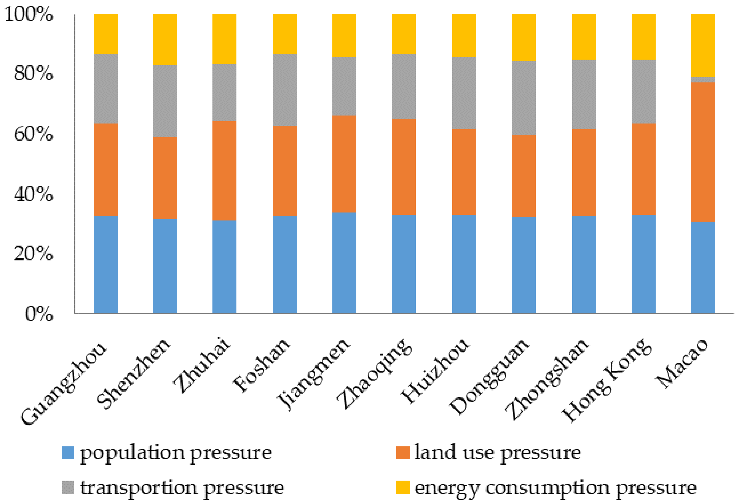
2.3.5. Cumulative Human Disturbance Intensity

Our research on the various human disturbance factors of the GBA did not involve specific weighting; therefore, to maintain research neutrality, the default weights of the four human disturbance indices were kept the same. The cumulative HDI score of grid i is the summation of the four human pressure scores. The expression is as follows:
H D I i = Nor P D I S i + Nor L D I S i + Nor T D I S i + Nor E D I S i .
The cumulative HDI was classified using Jenks natural breaks method into five HDI classes: very low, low, moderate, high, and very high.

2.4. Coastal Ecosystem Services System

Coastal ecosystems are composed of terrestrial, freshwater, wetland, and nearshore ecosystems. The coastal ES classification system was constructed based on the CICES [1]. The three categories and 12 subclasses of ES were identified from the aforementioned four types of ecosystems, and the ES sources were selected with reference to Li and Wang (2019) [42] (Table 4).
Provisioning services refer to the capacity of the environment to provide for the basic material needs of human survival and development, such as food, raw materials, and energy. Regulating and maintenance services refer to the role of the ecosystem in regulating and restoring the ecological security of the atmospheric, water, and soil environments through a series of ecological processes. Coastal wetlands (mangroves and coral reefs) can enhance the resilience of coastal zones under conditions of global climate change. Nature reserves are of great significance to protecting wildlife, forest ecology, inland wetlands, and ocean coasts [43]. Cultural services refer to the function of the ecological system as a carrier of esthetic value and historical culture, a place for scientific research, and education. Natural attractions, forest parks, and zoos have high natural ornamental value and scientific research and educational value [44]. Coastal bathing beaches provide residents with a place for leisure.
Points of interest cover the location and attribute information of varied geographic entities [45]. The ES sources were extracted from Amap using OSpider 2.1 on an administrative unit. The accuracy was calculated to be >85% by observing the consistency between the service functions of the sample points of ES sources and reference points from Open Street Map (https://www.openstreetmap.org/ accessed on 18 March 2021); therefore, the mapping results can accurately reflect the spatial distribution characteristics of ES in the GBA. The kernel density estimation method does not make any assumptions regarding the data distribution. It is a method used to study the characteristics of data distribution from the data sample itself [46]. It can be used to intuitively analyze the degree of aggregation of the ES spatial number distribution. We used the natural breaks (Jenks) classification method for the partitioning of kernel density to determine the capacity level of the ES in the GBA.

2.5. Spatial Correlation

Ecological and societal processes and patterns have uneven and complex spatial distributions due to differences in geographic environments. A geographically weighted model can be used to explore this characteristic among different variables [47,48,49]. We calculated the geographically weighted Pearson correlation coefficient [50] to explore the local correlation between ES and HDI. The formula is as follows:
G W P C C = j = 1 n w i j x j x ¯ i y j y ¯ i j = 1 n w i j x j x ¯ i 2 j = 1 n w i j y j y ¯ i 2 ,
where GWPCC is the geographically weighted Pearson correlation coefficient of ES and HDI; x i and y i are the ES and HDI of the regression analysis point i, respectively; and x j and y j are the ES and HDI, respectively, of the neighboring point j. The number of nearest neighbors around observation point i is represented by n, and x ¯ i and y ¯ i are the geographically weighted mean value of ES and HDI of point i, respectively, which are calculated by the formulae:
x ¯ i = j = 1 n x j w i j / j = 1 n w i j ,
y ¯ i = j = 1 n y j w i j / j = 1 n w i j ,
w i j = 1 d i j / b 2 2 ,           d i j b                 0               ,           o t h e r w i s e
where wij is the weight at point j, dij is the distance between points i and j, and b is the bandwidth of the kernel function. A smaller bandwidth improves the accuracy of the spatial change of the result, whereas a larger bandwidth makes the result appear closer to the global model [50]. By comparing the experimental results, it was found that setting the bandwidth to 0.03 produced results that are more in line with the spatial pattern of ES and HDI in the GBA.
The geographically weighted Pearson correlation coefficient ranged from −1 to 1. A positive value indicates a positive spatial correlation between ES and HDI, whereas a negative value indicates a negative spatial correlation. The greater the absolute value of the correlation coefficient, the stronger the spatial correlation between the ES and HDI.

2.6. Local Spatial Autocorrelation

Spatial autocorrelation analysis considers the relationship among spatially adjacent quantities. Bivariate local Moran analysis was performed in GeoDa V.1.12 to generate a local indicator of spatial association (LISA) cluster map, explore the spatial clustering patterns of ES and HDI, and verify their spatial autocorrelation. The clustering patterns were categorized into four types: high ES surrounded by high HDI (HH), high ES surrounded by low HDI (HL), low ES surrounded by high HDI (LH), and low ES surrounded by low HDI (LL).

3. Results

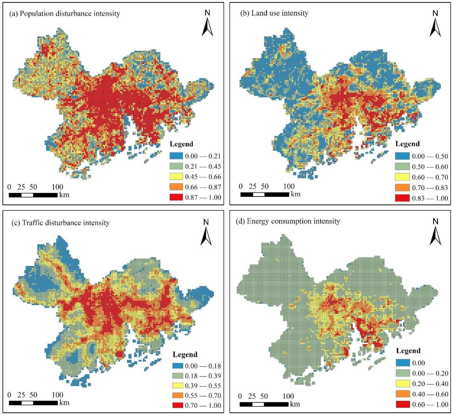
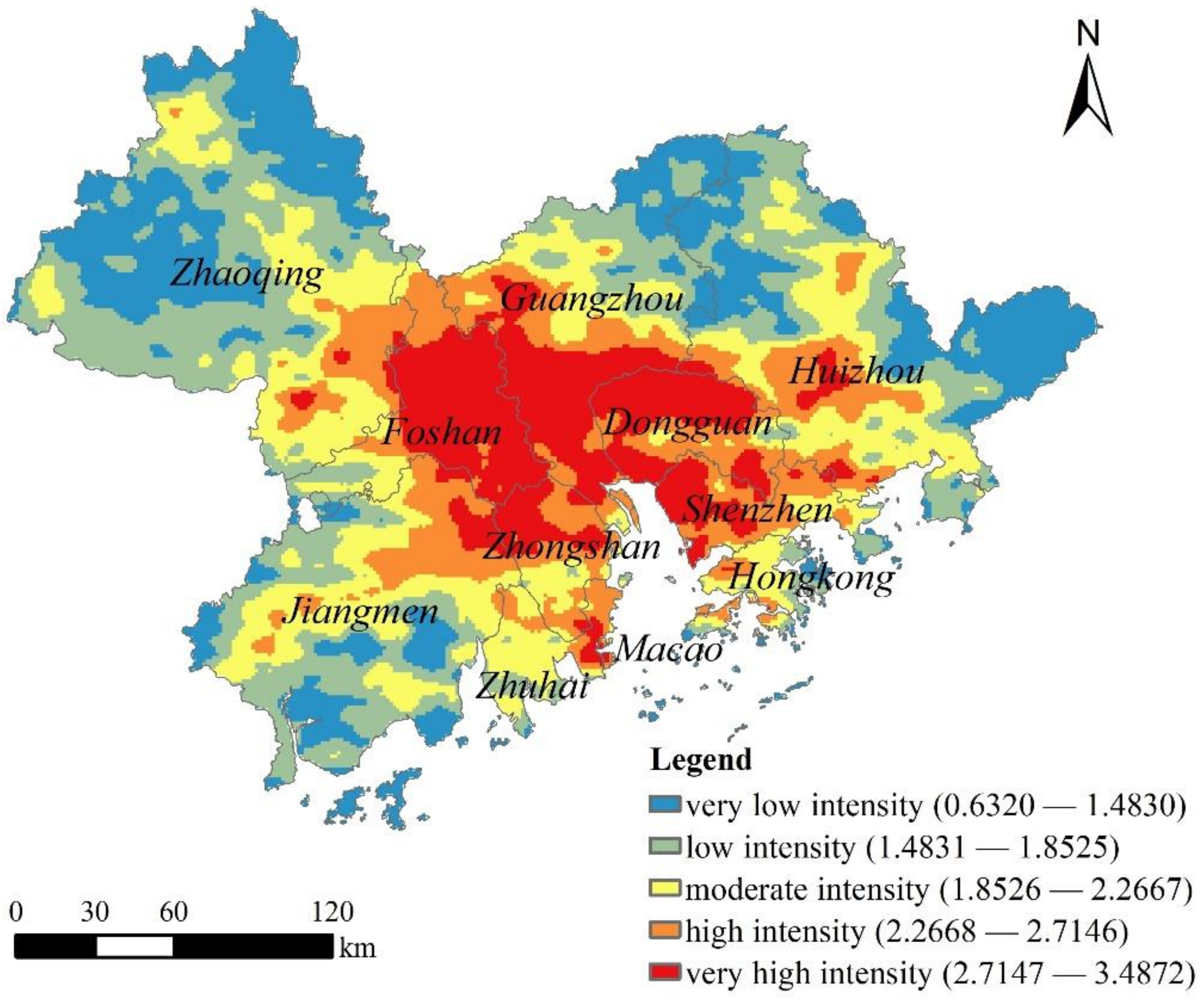
3.1. Spatial Patterns of Human Disturbance Intensity

Figure 3 demonstrates that human disturbances are unevenly distributed in the GBA. The strongest population disturbance is measured in the central cities (Hong Kong, Macao, Shenzhen, and Guangzhou); intermediate pressure is measured in Foshan, Zhongshan, Dongguan, and Zhuhai; and low pressure is measured in Jiangmen, Huizhou, and Zhaoqing (Figure 3a). The central cities are dominated by highly connected areas of built-up land, whereas cultivated land, garden land, and woodland are mainly distributed around the central cities and the periphery of the GBA. Built-up land exerts greater pressure on the ecological environment than other land types (Figure 3b). The traffic network system is radially distributed about the central cities. The intensity of traffic pressure in Guangzhou, Shenzhen, Foshan, and Huizhou is relatively high as compared to other cities (Figure 3c). The energy consumption of the central cities is significantly higher than that of the peripheral areas (Figure 3d). Central cities are international metropolises characterized by intense human activities and require huge amounts of energy to maintain their normal operations.
The center of the GBA is mainly dominated by moderate, high, and very high levels of HDI (Figure 4); these account for 22.33%, 15.92%, and 14.84% of the total intensity, respectively. The proportions of very low and low-intensity human disturbance are 21.95%, and 24.96%, respectively. The central and southern parts of the GBA are characterized by very high levels of human disturbance, especially in Guangzhou, Shenzhen, Zhuhai, Foshan, Dongguan, Zhongshan, Hongkong, and Macao, with mean HDI of 1.77, 2.38, 1.80, 2.00, 2.68, 2.35, 2.11, and 1.99, respectively. Some areas of Huizhou are characterized by medium and strong disturbance levels, whereas others exhibit only slight disturbance. Jiangmen and Zhaoqing have moderate and lower levels of disturbance, with mean HDI of 1.48, and 1.30, respectively. A very high-intensity disturbance in Guangzhou is distributed over its southern region. Most of the human disturbance in Hong Kong is of moderate or high intensity, but the average disturbance intensity score in its coastal segment is low. Levels of HDI are unevenly distributed over the GBA, as well as within the smaller administrative scale.
The contribution of each human pressure to the cumulative HDI was used to identify the leading contributors that affect the HDI level in the administrative area. Most cities are mainly affected by population density and intense land development (Figure 5). Compared with other disturbance factors, the population pressure of all municipal administrative regions is more prominent, and the population pressure of Guangzhou and Shenzhen is the most significant. The contribution of land-use pressure to the HDI of Guangzhou, Shenzhen, Zhuhai, Hong Kong, and Macao is relatively large at 30.83%, 27.42%, 33.03%, 30.24%, and 46.35%, respectively. The pressure of the traffic system provides greater contribution to the HDI in Guangzhou, Shenzhen, Foshan, Zhaoqing, Huizhou, Dongguan, and Zhongshan. Compared with other cities, Macao has higher energy consumption pressure.

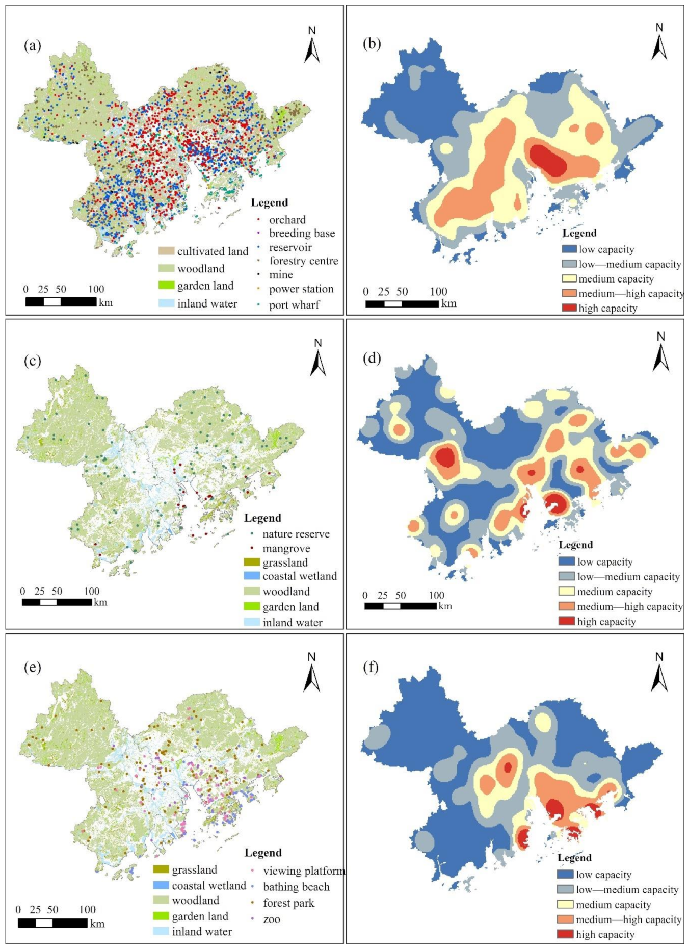
3.2. Spatial Distribution Characteristics of Ecosystem Services

In the GBA, the delivery of food and nutrients is concentrated in the central built-up area and nearby vicinity with high population density (Guangzhou, Shenzhen, Zhuhai, Dongguan, and Foshan). The commercial forests and mineral resources are mostly distributed in Zhaoqing, Jiangmen, and Huizhou. Jiangmen and Dongguan provide the water and power resources necessary for human life and production (Figure 6a). The high- and medium-high-capacity areas of provisioning services account for 2.50% and 17.58% of the total area, respectively (Table 4). Medium capacity areas account for 26.30% of the total area, and low-medium and low-capacity areas account for 26.74%, and 26.88%, respectively. From a spatial perspective, the provisioning services originate from the periphery of the central cities (Figure 6b). Guangzhou, Shenzhen, Dongguan, Foshan, Jiangmen, and Huizhou have relatively high provisioning service value.
Mangrove ecosystems are mainly distributed in Guangzhou, Shenzhen, Zhuhai, Zhongshan, Jiangmen, and Huizhou (Figure 6c). The high- and medium-high- capacity areas of regulating and maintenance services account for 2.43% and 11.62% of the total area, respectively; the areas of medium capacity levels of regulating and maintenance services account for 19.36%. The low-medium and low-capacity areas account for 31.21%, and 35.38%, respectively. From a spatial perspective, the regulating and maintenance services show high density in the outermost periphery of the GBA (Figure 6d). The high and medium-high-capacity areas for regulating and maintenance services are distributed in the coastal areas of Guangzhou, Shenzhen, Zhuhai, Zhongshan, Zhaoqing, and Huizhou.
Leisure and sightseeing services are mostly distributed over the periphery of the central urban built-up areas and along the coastline (Zhuhai, Shenzhen, and Hong Kong). Cultural, scientific research, and education services are concentrated in the central cities that have relatively complete public service infrastructures (Figure 6e). The areas of high and medium-high-capacity levels of cultural services account for 2.29%, and 8.74% of the total area, respectively (Table 5); cultural services are highly concentrated in the heartland of the GBA (Figure 6f). Medium capacity areas for cultural services account for 9.98% of the total area; low-medium and low-capacity cultural service areas account for 25.04%, and 53.95%, respectively.

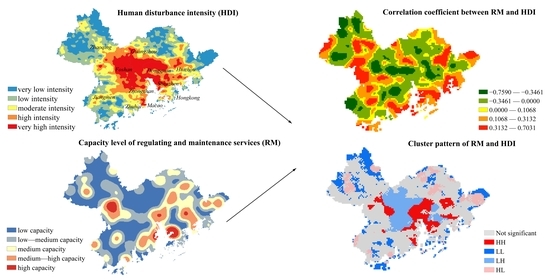
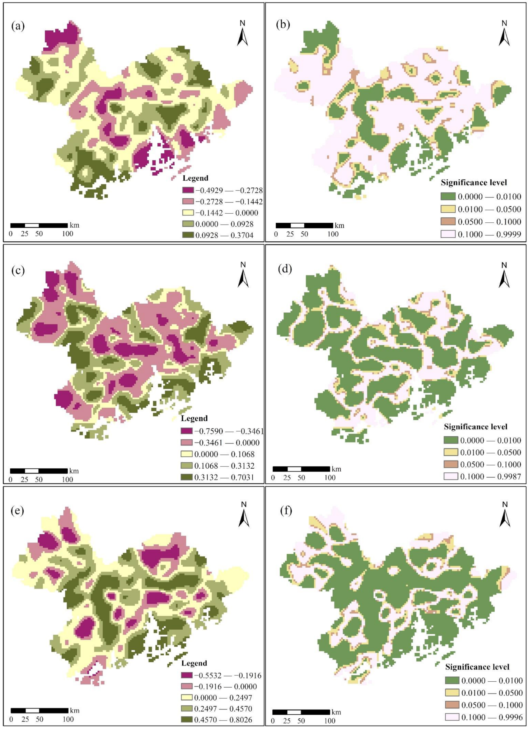
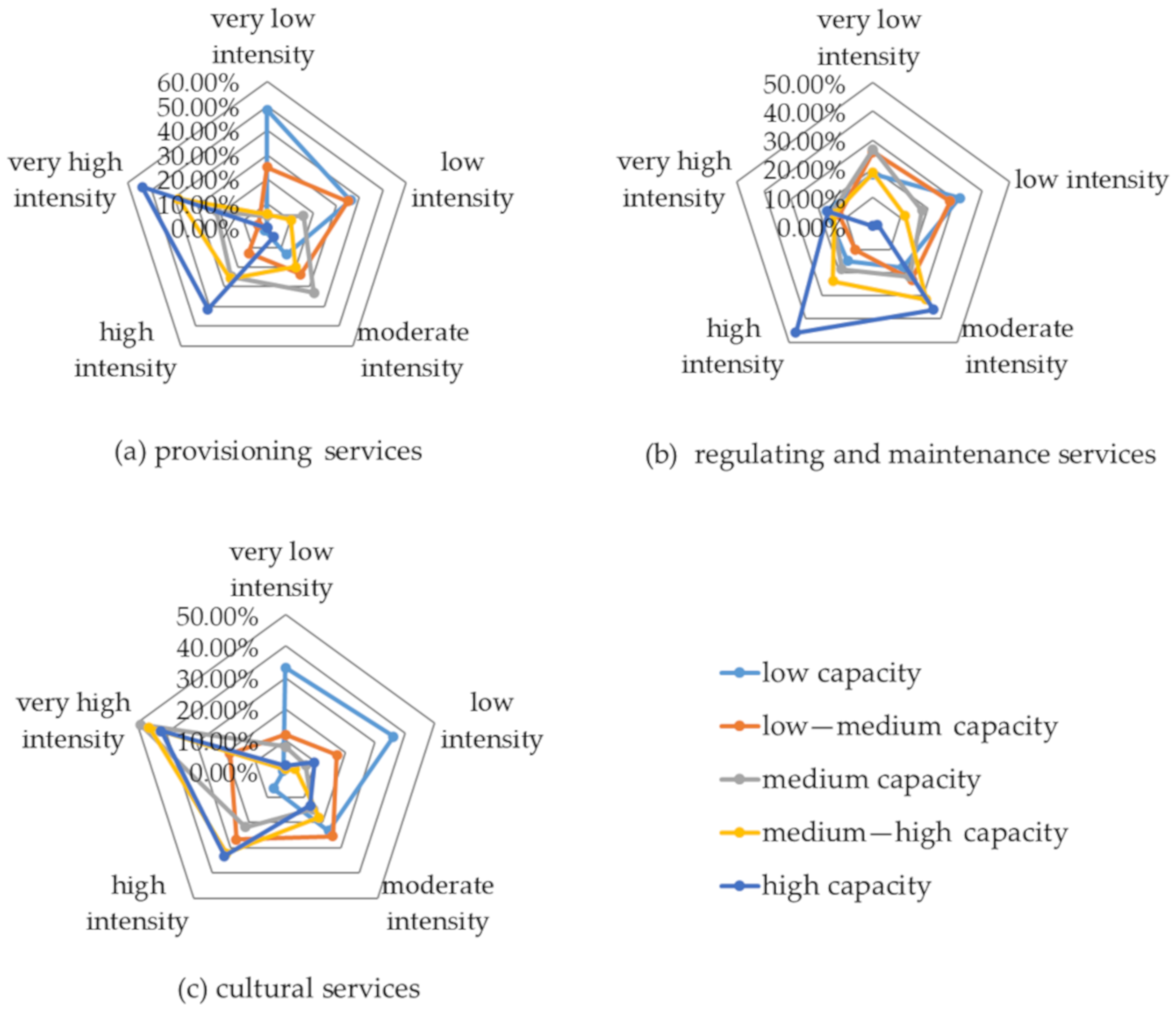
3.3. Spatial Correlations between Ecosystem Services and Human Disturbance Intensity

The global bivariate Moran shows the strong negative correlation between provisioning services and HDI (bivariate Moran’s I: −0.2399, P < 0.01). The positive correlation is strongest between cultural services and HDI (bivariate Moran’s I: 0.4784, P < 0.01), followed by that between regulating and maintenance services and HDI (bivariate Moran’s I: 0.1665, P < 0.01).
The spatial patterns of the local correlations between ES and HDI are shown in Figure 7. There is significant negative correlation between provisioning services and HDI in Guangzhou’s central urban area, Shenzhen’s coastal zone, Foshan, Zhuhai, Hong Kong, Macao, and the north of Zhaoqing (Figure 7a,b). There is significant positive correlation in most of Zhongshan, Dongguan, Zhaoqing, Jiangmen, and Huizhou. There is significant negative correlation between RM and HDI in the coastal areas of Guangzhou, Shenzhen, Zhuhai, Zhongshan, and most areas of Zhaoqing, Jiangmen, and Huizhou (Figure 7c,d). Regulating and maintenance services degrade as human disturbance increase. There is significant positive correlation between CS and HDI in Guangzhou, Shenzhen, Zhuhai, Foshan, Huizhou, Hong Kong, and Macao (Figure 7e,f). The results show that highly developed, densely populated areas have more demand for cultural, educational, leisure, and entertainment services. Therefore, cultural services are highly exploited in these cities, and the density of cultural services increase as human disturbance increase.
A quantitative analysis was conducted on the area of space overlap for each capacity level of ES under different levels of HDI using the “tabulate area grid” statistical tool in ArcGIS 10.4 (Figure 8). The medium-high and high-capacity regions of ES in the GBA are mainly under high and very high HDI, respectively. A proportion of 46.56% medium capacity areas, 64.00% medium-high-capacity areas, and 95.25% high-capacity areas of provisioning services are affected by high and very high HDI. Over half of the medium capacity areas, medium-high, and high-capacity areas of regulating and maintenance services are under high and very high HDI. Among these, 62.36% are high-capacity areas affected by high to very high HDI. There are 45.42% low-medium regions, 70.57% medium capacity regions, 77.92% medium-high-capacity regions, and 75.02% high-capacity regions of cultural services, respectively, and these regions are influenced by high and very high HDI. Most of the low-capacity regions are under very low, low, or medium HDI.

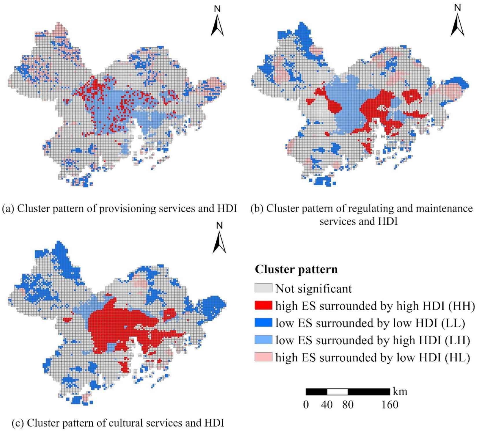
3.4. Spatial Cluster Pattern of Ecosystem Services (ES) and Human Disturbance Intensity (HDI)

The LISA cluster map of bivariate local Moran describes the clustering patterns of ES and HDI (Figure 9). The clustering patterns of provisioning services and HDI are relatively scattered, and H(provisioning services)H areas are widely distributed in the periphery of the urban center. The L(provisioning services)H areas are most concentrated in the city center (Hong Kong, Macao, Shenzhen, and Guangzhou; Figure 9a). H(regulating and maintenance services)H areas are mainly clustered in the coastal area, and in parts of Foshan and Huizhou. The L(regulating and maintenance services)H areas are most concentrated in the center of the GBA (Figure 9b). For cultural services, the H(cultural services)H areas are distributed across a large area and concentrated in the central cities of the GBA; L(cultural services)H goes around the periphery of central cities (Figure 9c). There are similarities in the cluster patterns of LL and HL among the three ES groups. They are scattered across the edge of the GBA with different degrees of aggregation; the most obvious aggregation is for cultural services, followed by regulating and maintenance services, and provisioning services. The spatial patterns of insignificant areas are similar in all LISA cluster maps; they are mainly distributed in the periphery of the central cities due to relatively fewer human activities (e.g., population aggregation, land development, and infrastructure construction) in these areas in comparison to the metropolitan area of the GBA.

4. Discussion

4.1. Mechanism of Interactions between Human Disturbance and Ecosystem Services

A large number of job opportunities, platforms, and policies for supporting business startups and innovation, and complete infrastructural facilities for living and production attract people to the GBA. However, the GBA is facing the problem of increased differentiation of population quantity. Of the 1.5 million population increment in the Pearl River Delta region in 2018, Guangzhou and Shenzhen account for 0.40 million and 0.49 million, respectively. The populations of Foshan and Zhuhai are also growing notably, whereas the remaining five cities only saw population increments in the tens of thousands [30].
Most natural land has been converted to built-up land to meet the demand of urbanization and industrialization. For many years, coastal areas and offshore islands have been subjected to continuous reclamation projects, and terrestrial and marine resources have been utilized with high intensity [51]. Built-up land covers an area of 6769.17 km2, which accounts for 12.18% of the total land area. It is mainly distributed over Guangzhou, Shenzhen, Hong Kong, and Macao.
The GBA has a complete transportation infrastructure and a dense road network in a radial distribution from the central cities to the surrounding areas. Foshan and Dongguan are making efforts to build a modern three-dimensional comprehensive transportation hub and accelerate the flow of people, logistics, capital, and information to the second-and third-tier cities; the first-tier cities are developing a hub-based economy in an effort to promote regional balance [52].
Shenzhen, Dongguan, Hong Kong, and Macao have highly developed economies and industries that require large energy resources to maintain daily operations. Compared with the light brightness value of other regions and highly populated bay areas, the degree of connectivity of the night-time lights of the GBA is significantly higher than that of the Tokyo Bay Area or the Yangtze River Delta urban agglomeration. The night-time light blocks are completely integrated, which indicates that the degree of urban integration in the GBA has reached a high level.
It can be seen from the aforementioned analysis that population and traffic pressure are the dominant factors of HDI in Guangzhou, Shenzhen, Dongguan, Foshan, Jiangmen, and Huizhou; there are greater material needs here and they are convenient for the delivery of provisioning services. The high- and medium-high-capacity areas of regulating and maintenance services are mainly distributed in the coastal areas of Guangzhou, Shenzhen, Zhuhai, Zhongshan, Zhaoqing, and Huizhou; these areas are mainly affected by the pressure from dense population and intense land-use. Cultural services are highly developed in Guangzhou, Shenzhen, Hong Kong, and Macao and the coastal zone of Zhuhai and Dongguan, where educational resources and recreational facilities are in great demand due to high-density population and highly developed economies. There is a complex feedback mechanism between human interference and ES. Human activities have positive effects on provisioning services and cultural services. Conversely, they can weaken the regulating and maintenance services, which will in turn impose restrictions on the delivery of provisioning services and cultural services. Areas with abundant ES are more conducive to carrying out various social and economic activities than areas with poor ecological functions.

4.2. Implications for Regional Planning

Implementing human activities without adversely affecting the sustainability of ecosystems, and minimizing the pressure on ES has been an essential concern for decision-makers worldwide. The current planning for developing functional zones attempts to alleviate the ecological environmental risks by directly delineating ecological protection areas in areas with a high concentration of ES, ecologically sensitive and fragile areas, and prohibiting or restricting economic and social activities. However, the study demonstrates that there is significant correlation between ES and HDI in the GBA, and that the existing planning overlooks the positive feedback between human activities and ES. Therefore, we should consider ES and human activities holistically and consider their interactions to minimize the negative impact on the natural environment and maximize ES value. Areas with high population density and high capacity for provisioning services and cultural services can be considered as ecological development zones for making full use of potential ecological values under the premise of priority protection. Areas with high capacity for regulating and maintenance services should be regarded as key ecological protection areas, and the strictest ecological protection measures should be adopted. In L(regulating and maintenance services)H areas, the intensity of urban construction should be appropriately controlled, or the land-use types used should be adjusted to create ecological landscapes (such as artificial wetlands and urban green spaces) and alleviate the impact of human activities on the environment. In L(provisioning services, cultural services)L areas, appropriate ecological restoration projects can be adopted due to lack of good natural conditions and abundant resources. Appropriate construction can be carried out to enhance their development vitality.
Urban planning and ecological landscape planning should be focused on H(regulating and maintenance services)H areas. From the perspective of spatial correlation, most high-capacity areas of regulating and maintenance services are under high HDI. The natural habitats with important ecological value in coastal regions (i.e., mangrove wetlands, coral reef wetlands, and seagrass beds) are affected by intense human activities (i.e., aquaculture, fishing, foreign trade, shipping port transportation, and leisure tourism). For example, the Halophila beccarii Asch seagrass bed in Tangjiawan, Zhuhai, can lessen the impact of waves, consolidate the coastline, and protect seabed geology. At present, the seagrass beds are rapidly decreasing owing to high-intensity human activities [53]. National nature reserves such as Xiangtou Mountain in Huizhou and Daya Bay in the South China Sea have also become tourist attractions. A high HDI will cause the loss of regulating and maintenance services and lead to further weakening of other ES. Hence, it is necessary to coordinate the scope of human activities and minimize adverse effects on natural ecosystems. The intensity and types of human activities in areas with high regulating and maintenance services value should be strictly controlled to avoid degradation of ecological resilience.
Human disturbance not only affects ES in the area where disturbance occurs but it will also lead to changes of ecological value in surrounding areas through the exchange of energy and materials with neighboring regions via natural processes, such as hydrological and atmospheric movements [54,55]. The LISA cluster map demonstrates that H(provisioning services, cultural services)H agglomerated in the center city of the GBA and large areas of L(provisioning services, cultural services)H cluster in its the neighboring cities, which indicates that there is a negative spillover effect in the spatial relationship between ES and HDI [56]. The high-capacity region for provisioning services and cultural services can lose its functions due to surrounding intense human disturbance. Therefore, we should avoid environmentally destructive activities around key ecological protection areas. Coastal wetlands have high capacity for regulating and maintenance services, whereas coastal zones are also H(regulating and maintenance services)H areas adjacent to the L(regulating and maintenance services)H areas. Intense human activities inevitably affect ES directly or indirectly in ecologically valuable areas. Therefore, land development and economic activities should be carefully planned in its surrounding areas.

4.3. Advances and Limitations

This study fills the knowledge gap of the interaction between human disturbance and coastal ecosystems. Compared with the global-scale research in inland regions, our study is more specific and targeted. We fully considered the characteristics of coastal areas, such as coastal wetlands and navigable waterways when selecting indicators of human disturbance factors. ES provided by coastal terrestrial ecosystems, wetland ecosystems, and nearshore ecosystems were also comprehensively considered, and the kernel density of ES sources were used to visualize the spatial distribution of ES hotspots more objectively compared with the calculation of ecological service values. Geographically weighted Pearson correlation coefficient and the bivariate local Moran can spatially visualize and quantitatively reflect the correlation between ES and HDI in local space compared with the previous methods (like linear regression).
There are still some limitations. Many human activities affect ES; however, we evaluated the regional HDI through only four types of human pressure. More specific human activities (i.e., consumption habits and types of industry, tourism pressure, types of energy consumed, and other specific mechanisms) that exert a considerable influence on ecosystems should also be explored. Additionally, we used 3 × 3 km grids as spatial units to study the spatial relationship between ES and HDI; this may generalize or overlook some interactions that occur at smaller scales. Therefore, future research should use multiscale grid units or administrative units for evaluation in order to obtain more comprehensive and reliable results.

5. Conclusions

We quantitatively explored and visualized the spatial correlation between human disturbance intensity and ecosystem services in the Guangdong–Hong Kong–Macao Greater Bay Area. The major findings are summarized as follows.
The central and southern regions of the Guangdong–Hong Kong–Macao Greater Bay Area are under intense human disturbance. The kernel density of ecosystem service sources can spatially and objectively manifest the capacity degree of ecosystem services. Provisioning services mainly originate from the outer edge of the central cities. Cultural services are highly concentrated in the central cities of the study area. Regulating and maintenance services have higher density in the outermost peripheries of the Guangdong–Hong Kong–Macao Greater Bay Area. High-capacity regions of ecosystem services are mainly under high intensity of human disturbance. Regions with high provisioning service values are mainly under the pressures of population and traffic, whereas regulating and maintenance services and cultural services are mainly dominated by high-density populations; regulating and maintenance service values are also affected by land-use pressure.
The global correlation analysis shows that provisioning services are significantly negatively correlated with human disturbance intensity, whereas a positive correlation is strongest between cultural services and human disturbance intensity, followed by that between regulating and maintenance services and human disturbance intensity. However, the correlation between human disturbance intensity and ecosystem services is spatially nonstationary when examined locally. This spatial heterogeneity is influenced by specific human activities, natural conditions, and management mechanism in local area.
Human disturbance has negative spillover effects on ecosystem services, which requires avoiding destructive activities around key ecological protection areas. It is of great significance to identify the spatial correlation between ecosystem services and human disturbance intensity for maintaining ecological resilience, optimizing coastal ecological planning, and improving resources allocation to ensure more equitable access among areas.

Author Contributions

Conceptualization and methodology, Y.H. and Y.K.; Data processing and analysis, Y.H. and Z.R.; Writing and draft preparation, Y.H.; Writing, reviewing, and editing, Y.H., Y.Z. and Y.K. All authors have read and agreed to the published version of the manuscript.

Funding

This research was supported by Science and Technology Planning Project of Guangdong Province, China (Nos: 2016A020228009), and Talent Introduction Project of Jinan University.

Institutional Review Board Statement

Not applicable.

Informed Consent Statement

Not applicable.

Data Availability Statement

Publicly available datasets were analyzed in this study. This data can be found here: [https://www.eastview.com/resources/e-collections/landscan/ accessed on 18 March 2021], [https://www.usgs.gov/ accessed on 18 March 2021], and [https://www.webmap.cn/commres.do?method=result100W accessed on 18 March 2021].

Acknowledgments

We would like to take this opportunity to acknowledge the time and effort devoted by reviewers to improving the quality of our paper.

Conflicts of Interest

The authors declare no conflict of interest.

References

  1. Haines-Young, R.; Potschin, M. Proposal for a Common International Classification of Ecosystem Goods and Services (CICES) for Integrated Environmental and Economic Accounting (V1). Report to the EEA. 2010. Available online: http://unstats.un.org/unsd/envaccounting/ceea/meetings/UNCEEA-5-7-Bk1.pdfS (accessed on 13 January 2021).
  2. Caro, C.; Marques, J.C.; Cunha, P.P.; Teixeira, Z. Ecosystem services as a resilience descriptor in habitat risk assessment using the InVEST model. Ecol. Indic. 2020, 115, 106426. [Google Scholar] [CrossRef]
  3. Costanza, R.; d’Arge, R.; de Groot, R.; Farber, S.; Grasso, M.; Hannon, B.; Limburg, K.; Naeem, S.; O’Neill, R.V.; Paruelo, J.; et al. The value of the world’s ecosystem services and natural capital. Nature 1997, 387, 253–260. [Google Scholar] [CrossRef]
  4. Millennium Ecosystem Assessment (MA). Ecosystems and Human Well-Being: Synthesis; Island Press: Washington, DC, USA, 2005. [Google Scholar]
  5. Darvill, R.; Lindo, Z. The inclusion of stakeholders and cultural ecosystem services in land management trade-off decisions using an ecosystem services approach. Landsc. Ecol. 2016, 31, 533–545. [Google Scholar] [CrossRef]
  6. Wan, L.L.; Ye, X.Y.; Lee, J.; Lu, X.Q.; Zheng, L.; Wu, K.Y. Effects of urbanization on ecosystem service values in a mineral resource-based city. Habitat Int. 2015, 46, 54–63. [Google Scholar] [CrossRef]
  7. Zhang, Y.; Liu, Y.F.; Zhang, Y.; Liu, Y.; Zhang, G.X.; Chen, Y.Y. On the spatial relationship between ecosystem services and urbanization: A case study in Wuhan, China. Sci. Total Environ. 2018, 637–638, 780–790. [Google Scholar] [CrossRef] [PubMed]
  8. Rangel-Buitrago, N.; Neal, W.J.; Bonetti, J.; Anfuso, G.; de Jonge, V.N. Vulnerability assessments as a tool for the coastal and marine hazards management: An overview. Ocean Coast. Manag. 2020, 189, 105134. [Google Scholar] [CrossRef]
  9. Braat, L.C.; de Groot, R. The ecosystem services agenda: Bridging the worlds of natural science and economics, conservation and development, and public and private policy. Ecosyst. Serv. 2012, 1, 4–15. [Google Scholar] [CrossRef] [Green Version]
  10. Myers, N.; Mittermeier, R.A.; Mittermeier, C.G.; Gustavo, A.B.; da Fonseca, G.A.; Kent, J. Biodiversity hotspots for conservation priorities. Nature 2000, 403, 853–858. [Google Scholar] [CrossRef]
  11. Mahmoud, S.H.; Gan, T.Y. Impact of anthropogenic climate change and human activities on environment and ecosystem services in arid regions. Sci. Total Environ. 2018, 633, 1329–1344. [Google Scholar] [CrossRef]
  12. Sanderson, E.W.; Jaiteh, M.; Levy, M.A.; Redford, K.H.; Wannebo, A.V.; Woolmer, G. The human footprint and the last of the wild. Bioscience 2002, 52, 891–904. [Google Scholar] [CrossRef]
  13. Halpern, B.S.; Walbridge, S.; Selkoe, K.A.; Kappel, C.V.; Micheli, F.; D’Agrosa, C.; Bruno, J.F.; Casey, K.S.; Ebert, C.; Fox, H.E.; et al. A global map of human impact on marine ecosystems. Science 2008, 319, 948–952. [Google Scholar] [CrossRef] [PubMed] [Green Version]
  14. Venter, O.; Sanderson, E.W.; Magrach, A.; Allan, J.R.; Beher, J.; Jones, K.R.; Possingham, H.P.; Laurance, W.F.; Wood, P.; Fekete, B.M.; et al. Sixteen years of change in the global terrestrial human footprint and implications for biodiversity conservation. Nat. Commun. 2016, 7, 12558. [Google Scholar] [CrossRef] [PubMed] [Green Version]
  15. Tapia-Armijos, M.F.; Homeier, J.; Munt, D.D. Spatio-temporal analysis of the human footprint in South Ecuador: Influence of human pressure on ecosystems and effectiveness of protected areas. Appl. Geog. 2017, 78, 22–32. [Google Scholar] [CrossRef]
  16. Rogers, H.M.; Glew, L.; Honzák, M.; Hudson, M.D. Prioritizing key biodiversity areas in Madagascar by including data on human pressure and ecosystem services. Landsc. Urban Plan. 2010, 96, 48–56. [Google Scholar] [CrossRef]
  17. Li, S.C.; Wu, J.S.; Gong, J.; Li, S.W. Human footprint in Tibet: Assessing the spatial layout and effectiveness of nature reserves. Sci. Total Environ. 2018, 621, 18–29. [Google Scholar] [CrossRef] [PubMed]
  18. Mustafa, R.G.; Blaine, D.G. Diet, energy storage, and reproductive condition in a bioindicator species across beaches with different levels of human disturbance. Ecol. Indic. 2020, 117, 106636. [Google Scholar] [CrossRef]
  19. Peng, J.; Tian, L.; Liu, Y.X.; Zhao, M.Y.; Hu, Y.N.; Wu, J.S. Ecosystem services response to urbanization in metropolitan areas: Thresholds identification. Sci. Total Environ. 2017, 607–608, 706–714. [Google Scholar] [CrossRef]
  20. Han, R.; Feng, C.C.; Xu, N.Y.; Guo, L. Spatial heterogeneous relationship between ecosystem services and human disturbances: A case study in Chuandong, China. Sci. Total Environ. 2020, 721, 137818. [Google Scholar] [CrossRef]
  21. Qi, Y.; Lian, X.H.; Wang, H.W.; Zhang, J.L.; Yang, R. Dynamic mechanism between human activities and ecosystem services: A case study of Qinghai lake watershed, China. Ecol. Indic. 2020, 117, 106528. [Google Scholar] [CrossRef]
  22. Tang, G.T.; Yao, H.M.; Li, X.M.; Qin, N.J.; Gu, F.M. Review on Evaluation of Ecosystem Services. In Proceedings of the Conference on Environmental Pollution and Public Health (CEPPH 2012), Shanghai, China, 17–19 May 2012. [Google Scholar]
  23. Loreau, M.; Naeem, S.; Inchausti, P.; Bengtsson, J.; Grime, J.P.; Hector, A.; Hooper, D.U.; Huston, M.A.; Raffaelli, D.; Schmid, B.; et al. Biodiversity and ecosystem functioning: Current knowledge and future challenges. Science 2001, 294, 804–808. [Google Scholar] [CrossRef] [PubMed] [Green Version]
  24. Hu, M.M.; Li, Z.T.; Wang, Y.F.; Jiao, M.Y.; Li, M.; Xia, B.C. Spatio-temporal changes in ecosystem service value in response to land-use/cover changes in the Pearl River Delta. Resour. Conserv. Recycl. 2019, 149, 106–114. [Google Scholar] [CrossRef]
  25. General Office of the People’s Government of Guangdong Province. Integrated Planning of Ecological Security System in the Pearl River Delta Region (2014–2020). Available online: http://zwgk.gd.gov.cn/006939748/201412/t20141211_559384.html (accessed on 20 November 2020).
  26. Xu, Z.N.; Gao, X.L. A novel method for identifying the boundary of urban built-up areas with POI data. Acta Geogr. Sin. 2016, 71, 928–939. [Google Scholar]
  27. Tang, X.M.; Liu, Y.; Pan, Y.C. An Evaluation and Region Division Method for Ecosystem Service Supply and Demand Based on Land Use and POI Data. Sustainability 2020, 12, 2524. [Google Scholar] [CrossRef] [Green Version]
  28. Outline Development Plan for the Guangdong-Hong Kong-Macao Greater Bay Area. Available online: http://www.gov.cn/gongbao/content/2019/content_5370836.htm (accessed on 5 December 2020).
  29. Guangdong Statistical Yearbook. 2019. Available online: http://stats.gd.gov.cn/gdtjnj/content/post_2639622.html (accessed on 5 December 2020).
  30. National Bureau of Statistics. Available online: https://data.stats.gov.cn/easyquery.htm?cn=E0110 (accessed on 8 January 2021).
  31. Luo, D.; Zhang, W.T. A comparison of Markov model-based methods for predicting the ecosystem service value of land use in Wuhan, central China. Ecosyst. Serv. 2014, 7, 57–65. [Google Scholar] [CrossRef]
  32. Tolessa, T.; Senbeta, F.; Kidane, M. The impact of land use/land cover change on ecosystem services in the central highlands of Ethiopia. Ecosyst. Serv. 2017, 23, 47–54. [Google Scholar] [CrossRef]
  33. Chen, H.; Li, S.C.; Zhang, Y.L. Impact of road construction on vegetation alongside Qinghai-Xizang highway and railway. Chin. Geogr. Sci. 2003, 13, 340–346. [Google Scholar] [CrossRef]
  34. Elvidge, C.D.; Baugh, K.E.; Kihn, E.A.; Kroehl, H.W.; Davis, E.R.; Davis, D.W. Relation between satellite observed visible-near infrared emissions, population, economic activity and electric power consumption. Int. J. Remote Sens. 1997, 18, 1373–1379. [Google Scholar] [CrossRef]
  35. He, C.Y.; Ma, Q.; Liu, Z.F.; Zhang, Q.F. Modeling the spatiotemporal dynamics of electric power consumption in mainland China using saturation-corrected DMSP/OLS nighttime stable light data. Int. J. Digit. Earth 2014, 7, 993–1014. [Google Scholar] [CrossRef]
  36. Shi, K.F.; Chen, Y.; Yu, B.L.; Xu, T.B.; Yang, C.S.; Li, L.Y.; Huang, C.; Chen, Z.Q.; Liu, R.; Wu, J.P. Detecting spatiotemporal dynamics of global electric power consumption using DMSP-OLS nighttime stable light data. Appl. Energ. 2016, 18, 450–463. [Google Scholar] [CrossRef]
  37. East View. Landscan Global Population Database—East View. 2021. Available online: https://www.eastview.com/resources/e-collections/landscan/ (accessed on 7 January 2021).
  38. United States Geological Survey. Available online: https://www.usgs.gov/ (accessed on 7 January 2021).
  39. China National Catalogue Service for Geographic Information. 1:1,000,000 National Basic Geographic Database. Available online: https://www.webmap.cn/commres.do?method=result100W (accessed on 8 January 2021).
  40. Brentrup, F.; Kusters, J.; Lammel, J.; Kuhlmann, H. Life cycle impact assessment of land use based on the hemeroby concept. Int. J. Life Cycle Assess. 2002, 7, 339–348. [Google Scholar] [CrossRef]
  41. Rüdisser, J.; Tasser, E.; Tappeiner, U. Distance to nature—A new biodiversity relevant environmental indicator set at the landscape level. Ecol. Indic. 2012, 15, 208–216. [Google Scholar] [CrossRef]
  42. Li, J.X.; Wang, J. Identification, classification, and mapping of coastal ecosystem services of the Guangdong, Hong Kong, and Macao Great Bay Area. Acta Ecol. Sin. 2019, 39, 6393–6403. (In Chinese) [Google Scholar]
  43. Chen, Y.H.; Zhang, J.; Jiang, J.P.; Nielsen, S.E.; He, F.L. Assessing the effectiveness of China’s protected areas to conserve current and future amphibian diversity. Divers. Distrib. 2017, 23, 146–157. [Google Scholar] [CrossRef]
  44. Qiu, L.; Lindberg, S.; Nielsen, A.B. Is biodiversity attractive?—On-site perception of recreational and biodiversity values in urban green space. Landsc. Urban Plan. 2013, 119, 136–146. [Google Scholar] [CrossRef]
  45. Bao, J.; Xu, C.; Liu, P.; Wang, W. Exploring bikesharing travel patterns and trip purposes using smart card data and online point of interests. Netw. Spat. Econ. 2017, 17, 1231–1253. [Google Scholar] [CrossRef]
  46. Cai, W.M.; Xiao, T.; Bi, F.Y.; Shi, Y.Z. Analysis of spatial distribution characteristics of cultivated land based on kernel density estimation in metropolis—A case study in Tianjin. Chin. J. Agri. Resour. Region. Plan. 2019, 40, 152–160. (In Chinese) [Google Scholar]
  47. Fotheringham, A.S.; Brunsdon, C.; Charlton, M. Geographically Weighted Regression—The Analysis of Spatially Varying Relationships; Wiley: Chichester, UK, 2002. [Google Scholar]
  48. Brunsdon, C.; Fotheringham, A.S.; Charlton, M. Geographically weighted summary statistics—A framework for localised exploratory data analysis. Comput. Environ. Urban Syst. 2002, 26, 501–524. [Google Scholar] [CrossRef] [Green Version]
  49. Harris, P.; Brunsdon, C. Exploring spatial variation and spatial relationships in a freshwater acidification critical load data set for Great Britain using geographically weighted summary statistics. Comput. Geosci. 2010, 36, 54–70. [Google Scholar] [CrossRef]
  50. Kalogirou, S. A spatially varying relationship between the proportion of foreign citizens and income at local authorities in Greece. In Proceedings of the 10th International Congress of the Hellenic Geographical Society, Aristotle University of Thessaloniki, Thessaloniki, Greece, 22–24 October 2014. [Google Scholar]
  51. Liu, Y.S.; Wang, L.J.; Long, H.L. Spatio-temporal analysis of land-use conversion in the eastern coastal China during 1996–2005. J. Geogr. Sci. 2008, 18, 274–282. [Google Scholar] [CrossRef]
  52. Foshan Daily. Foshan Strives to Build a Modern Three-Dimensional Comprehensive Transportation Hub. Available online: https://www.foshannews.net/fstt/202009/t20200914_349193.html (accessed on 5 December 2020).
  53. Qiu, G.L.; Su, Z.N.; Fan, H.Q.; Fang, C.; Chen, S.T. Biological and ecological characteristics of intertidal seagrass Halophila beccarii and its conservation countermeasures. Mar. Environ. Sci. 2020, 39, 121–126. (In Chinese) [Google Scholar]
  54. Burkhard, B.; Kandziora, M.; Hou, Y.; Müller, F. Ecosystem service potentials, flows and demands—Concepts for spatial localisation, indication and quantification. Landsc. Online 2014, 34, 1–32. [Google Scholar] [CrossRef]
  55. Groot, R.S.D.; Alkemade, R.; Braat, L.; Hein, L.; Willemen, L. Challenges in integrating the concept of ecosystem services and values in landscape planning, management and decision making. Ecol. Complex. 2010, 7, 260–272. [Google Scholar] [CrossRef]
  56. Day, J.; Lewis, B. Beyond univariate measurement of spatial autocorrelation: Disaggregated spillover effects for Indonesia. Cartogr. Geogr. Inf. Sci. 2013, 19, 169–185. [Google Scholar] [CrossRef]
Figure 1. Location and scope of the study area.
Remotesensing 13 01174 g001
Figure 2. Research steps of this study.
Remotesensing 13 01174 g002
Figure 3. Intensity scores of each human pressure in the Guangdong–Hong Kong–Macao Greater Bay Area (GBA) (2018).
Remotesensing 13 01174 g003
Figure 4. Map of intensity levels of cumulative human disturbance in the Guangdong–Hong Kong–Macao Greater Bay Area (GBA).
Remotesensing 13 01174 g004
Figure 5. Contribution of each human pressure to the human disturbance intensity (HDI) level by administrative area.
Remotesensing 13 01174 g005
Figure 6. Spatial pattern of ecosystem services (ES) and spatial division by capacity level: (a) spatial pattern of provisioning services; (b) capacity level of provisioning services; (c) spatial pattern of regulating and maintenance services; (d) capacity level of regulating and maintenance services; (e) spatial pattern of cultural services; and (f) capacity level of cultural services.
Remotesensing 13 01174 g006
Figure 7. Geographically weighted Pearson correlation coefficient (GWPCC) between ecosystem services (ES) and human disturbance intensity (HDI) and the level of significance test: (a) GWPCC between provisioning services and HDI; (b) significance test for GWPCC between provisioning services and HDI; (c) GWPCC between regulating and maintenance services and HDI; (d) significance test for GWPCC between regulating and maintenance services and HDI; (e) GWPCC between cultural services and HDI; and (f) significance test for GWPCC between cultural services and HDI. Statistically significant at the 1% level.
Remotesensing 13 01174 g007
Figure 8. Distribution of capacity levels of ecosystem services (ES) under different human disturbance intensity (HDI).
Remotesensing 13 01174 g008
Figure 9. Bivariate LISA cluster maps of ecosystem services (ES) and human disturbance intensity (HDI).
Remotesensing 13 01174 g009
Table 1. Multi-source remote sensing data used in the study.
Data NameData TypeSpatial Resolution/ScaleSource
Population density dataRemote sensing data1 km gridLandScan Global Population Database, Department of Energy, Oak Ridge National Laboratory [37]
Landsat 8 OLI/TIRS images Remote sensing data30 mUnited States Geological Survey [38]
Road network vector dataVector data1:1,000,000China National Catalogue Service for Geographic Information [39]
VIIRS night-time lights imageRemote sensing data500 mGoogle Earth Engine (GEE, https://code.earthengine.google.com accessed on 18 March 2021)
Table 2. Land-use types and land-use intensity scores assigned to each type.
Land-Use TypeDescriptionDisturbance IntensityScore
Built-up landLand for urban uses, including factories, quarries, mining, transportation facilities, and airportexcessive 10
Rural settlementLand used for settlements in villages very strong 8
Cultivated landLand mainly for growing cropsstrong 6
Garden landUnformed forest afforestation land, nursery, and various garden land 6
Inland waterNatural inland waters, and land for water conservancy facilities, including rivers, lakes, reservoirs, ponds, etc.moderate 4
GrasslandArea dominated by herbaceous plants of natural growth and artificial planting 4
WoodlandTracts of natural forest, secondary forest, and artificial forestWeak2
Coastal wetlandDepressions in the coastal area that has been in a state of standing water or semi-water for a long time, including beaches, swamps, mangroves, etc.Slight1
Unused landNot put into practical use or is difficult to use, including sandy land, saline land, swampland, bare soil, bare rock, and othersAlmost no disturbance0
Table 3. Traffic disturbance intensity scores.
Type0–1 km1–5 km5–10 km10–15 km
Expressway10875
First-grade highway10842
Secondary highway8620
Tertiary highway6410
Fourth-class highway4200
Substandard way2100
Rural road1000
Railway9753
Navigable waterway7510
Table 4. Ecosystem service classification system and the ecosystem service sources of the GBA.
Main CategorySubclassSpecific ContentES Source
Provisioning servicesNutrition and essential substancesTerrestrial and aquatic animal and plant food, drinking waterOrchard, breeding base, reservoir
Raw materialBiological and non-biological materials (e.g., wood, rubber)Forestry center
Energy sourcesRenewable biofuels and non-bioenergy (such as minerals, geothermal resources, hydropower, solar energy)Mine (including geothermal energy),
power station
OtherCarrier of other service functions (such as transport carrier)Port wharf
Regulating and maintenance servicesHydrology regulation and water purificationIntercept, absorb, and store precipitation, regulate runoff; filter and decompose impurities and harmful chemicals, and promote the self-purification of the water Natural habitat
Climate regulation and air quality maintenancePromote the self-purification of the air, adjust the climate, and provide a climate suitable for human survivalNatural habitat
Soil conservation, wind break, and sand fixationRetain soil and slow down erosion; intercept and decompose organic matter, provide fertile land resources, and soil self-repair abilityNatural habitat
Habitat maintenance and biodiversity conservationProvide a stable habitat environment for organisms, carry out biological gene preservation, population maintenance, and new species breeding, and protect biodiversityNature reserve
Flood and tidewater control and shoreline stabilizationConfers resistance to disasters, adapt to disturbances, and maintain ecosystem stabilityMangrove, coral reef
Cultural servicesLandscapeAesthetic appreciation, recreation, and leisure travelObservation deck,
bathing beach,
forest park, zoo
Cultural carrierSpirit and culture contained in the ecosystem, such as history and religion
Scientific research and educationThe object of scientific research and education provides opportunities to understand, observe, and explore the ecosystem
Table 5. Summary statistics of the capacity level of ecosystem services (ES).
ClassificationProvisioning ServicesRegulating and Maintenance ServicesCultural Services
Area/km2Proportion/%Area/km2Proportion/%Area/km2Proportion/%
low capacity 14,93126.88%19,64735.38%29,96553.95
low-medium capacity14,84926.74%17,33431.21%13,90825.04
medium capacity14,60626.30%10,75319.36%55429.98
medium-high capacity976317.58%645311.62%48538.74
high capacity13892.50%13512.43%12702.29
Publisher’s Note: MDPI stays neutral with regard to jurisdictional claims in published maps and institutional affiliations.

