An Advanced Phase Synchronization Scheme Based on Coherent Integration and Waveform Diversity for Bistatic SAR

Abstract

In the bistatic synthetic aperture radar (BiSAR) system, the deviation between two oscillators in different platforms will cause an additional modulation of BiSAR echoes. Therefore, phase synchronization is one of the key issues that must be addressed for the BiSAR system. The oscillator phase error model and the principle of phase synchronization are firstly described. The waveform diversity technology has been widely used in many fields, for example, the hearing aids device and the recognition of auditory input source in cocktail party problem. Inspired by this, an advanced phase synchronization scheme based on coherent integration and waveform diversity is proposed. The synchronization signal and radar signal are orthogonal signals which can be separated by using waveform diversity technique. After extracting the synchronization signal, the phase synchronization accuracy can be further improved by coherent integration. The transmission of synchronization signals between two synchronization antennas is analyzed, followed by the theoretical error analysis. Then, the processing of separating the echo signal and synchronization signal is described in detail. The simulation experiments are performed. The accuracy of phase synchronization can reach 1 degree, which verifies the effectiveness of the proposed synchronization scheme.

1. Introduction

Synthetic aperture radar (SAR) is an active remote sensing instrument which can provide high-resolution two-dimensional images independent of sunlight illumination and weather conditions [1]. A number of SAR-derived techniques have been developed, such as repeat-pass interferometry, tomography SAR, polarimetric SAR and so on [2]. Although these techniques have been widely used for Earth observation, they have some inherent limitations in monostatic SAR mode. For example, repeat-pass interferometry suffers from two main difficulties, temporal decorrelation and atmospheric disturbances, which reduce the accuracy of digital elevation measurement [3]. However, these two difficulties can be avoided by using the bistatic SAR (BiSAR), which offer a natural way to implement single-pass interferometry. The BiSAR system, separated with transmitter and receiver, also has some other unique advantages, such as frequent monitoring, resolution enhancement and multi-angle scattering information, making it a promising and useful supplement to a classical monostatic SAR system [4].

The advantages of BiSAR system accompanies by new challenges. Phase synchronization is one of the most challenging problems [5,6]. In BiSAR system, the transmitter and receiver use different oscillators. There will be a frequency offset between oscillators of transmitter and receiver. Both the frequency offset and oscillator phase error will introduce phase error in the bistatic echo signal [7]. The phase error can be divided into three components: linear phase error, second-order phase error and higher-order phase error, causing linear displacement, mainlobe dispersion and increase of sidelobes respectively [8]. Therefore, phase synchronization is required to eliminate the phase error to guarantee the coherence of the transmitter and the receiver over an extremely long period of time.

Numerous synchronization schemes have been proposed in the last few decades. They can be divided into the following categories: clock based synchronization, parameter estimation based synchronization, direct-pulse based synchronization, continuous/pulsed duplex based synchronization, alternated-pulse based synchronization and some other synchronization schemes. Essentially, the phase error is caused by the inconsistency of clocks. Therefore, for clock based synchronization, a possible solution is using high accuracy and stable optical clocks. In the last few years, the optical clocks have achieved rapid development [9,10,11,12,13]. For example, two optical clocks with $4.8\times {10}^{-17}$ stability at 1 s is demonstrated in [13]. However, until a few years ago, optical clock technology has been tested in space for the first time [12]. There is still a big gap in the stable operation of the optical clock in the orbit. In parameter estimation based synchronization, the phase error is estimated by using the autofocus algorithm [14]. However, the accuracy of estimation is depended on the target in the scene, which limit its application. In direct-pulse based synchronization, the direct signal is received simultaneously with echoes. The direct signal can be regarded as a reference signal which can be used for phase synchronization [2,15]. However, the drawback of using direct signal is that the receiver antenna for direct signal must apper in the main beam of transmitter, which is not always fulfilled.

The continuous/pulsed based synchronization is proposed in [5] and has been further investigated in [6,16]. The alternated-pulse synchronization scheme is used in TanDEM-X [3] and the orbit verification and performance of it are introduced in [17,18]. The basic principle of alternated-pulsed synchronization scheme is to exchange the oscillator signals, which is somehow similar with microwave ranging [6], White Rabbit Network [19] and Two Way Time Transfer [20]. However, phase synchronization involved a dedicated processing approach. By exchanging the information between two systems, the phase error can be obtained to correct the bistatic echoes. In TanDEM-X, in order to exchange the synchronization signals between the two satellites, the nominal BiSAR data acquisition is periodically interrupted [3]. Since the missing raw data introduces artifacts in the processed images, recovery methods such as Papoulis-Gerchberg (PG) algorithm and Gapped Amplitude and Phase Estimation (GAPES) algorithm have been investigated in [21,22] to improve the quality of SAR image. The non-interrupted phase synchronization scheme, which can be regarded as an improved pulsed alternate synchronization scheme, is proposed for LuTan-1 mission [23,24,25,26]. The synchronization pulses are exchanged immediately after the ending time of the radar echo receiving window and before the starting time of the next pulse repetition interval (PRT) [25]. Therefore, it can not interrupt the normal SAR data acquisition, further improving synchronization frequency and avoiding the missing data effect. However, the non-interrupted synchronization scheme is based on the fact that the free time for synchronization transmission is enough in LuTan-1 mission [26]. Due to the limited time for synchronization pulses exchange, the pulse width of synchronization signal is less than the pulse width of radar signal. On the one hand, in order to reduce the influence on the range swath, the pulse width is expected to be as small as enough, on the other hand, the signal-to-noise ratio (SNR) will decrease if the pulse width decreases, which will reduce phase synchronization accuracy. Therefore, there is a trade-off between the pulse width and SNR [26].

Modern radar systems are increasingly being equipped with arbitrary waveform generators that enable simultaneous transmission of different waveform [27]. The waveform diversity technology has been widely used in many fields, for example, the hearing aids device and the recognition of auditory input source in cocktail party problem. In radar system, the waveform diversity is referred as adaptivity of the radar waveform to dynamically optimize the radar performance for the particular scenario and tasks [28]. For example, the up and down chirps are used for suppress of ambiguities [29,30]. The short-term shift-orthogonal waveforms are used for digital beamforming on receive [31] and nadir echo removal [32]. In this paper, an advanced phase synchronization scheme based on coherence integration and waveform diversity is proposed for the BiSAR system, which can acquire high accuracy synchronization phase without affecting the swath coverage. In the proposed synchronization scheme, the synchronization signal and radar signal are orthogonal signals, and the synchronization signal and SAR echoes are received simultaneously. Then, based on the waveform diversity concept, the synchronization signal and SAR echoes can be separated in the postprocessing. Besides, the synchronization accuracy can be further improved by coherent integration. A detail theoretical analysis is given in the paper and the simulation experiments are demonstrated to verify the effectiveness of the proposed scheme. The proposed synchronization scheme can avoid the influence of synchronization signal width on swath coverage, which can be regarded as an improved non-interrupted synchronization scheme.

This paper is organized as follows. Prior to introducing the synchronization scheme, we start with an introduction of principle of phase synchronization. The error analysis of phase synchronization is presented in Section 2.3. Then, in Section 2.4, the proposed synchronization is described in detail. The waveform diversity and coherent integration are presented. In Section 2.5, we present the processing of received signal, which includes extracting synchronization signal to obtain the synchronization phase, and removing the synchronization signal to obtain echoes. In Section 3, the simulation experiments are carried out to demonstrate the effectiveness of the proposed scheme. Section 4 concludes the paper.

2. Materials and Methods

2.1. Oscillator Phase Error Model

In this subsection, the model of oscillator phase error is introduced, which can be regarded as a foundation of phase synchronization.

In a BiSAR system, assume that $f_0$ is the nominal carrier frequency. However, the actual center carriers of primary satellite and slave satellite are derived from the ideal value. Suppose the actual center frequency of primary satellite and slave satellite are $f_1$ and $f_2$, respectively. The instantaneous phases of oscillators in primary satellite and slave satellite at time t can be written as follows [33]

$$\begin{array}{c}\hfill {\phi }_1\left(t\right)=2\pi f_{1}t+{\varphi }_1\left(t\right)+{\varphi }_1\end{array}$$

(1)

$$\begin{array}{c}\hfill {\phi }_2\left(t\right)=2\pi f_{2}t+{\varphi }_2\left(t\right)+{\varphi }_2\end{array}$$

(2)

where ${\varphi }_1\left(t\right)$ and ${\varphi }_2\left(t\right)$ are time-varying phase errors of primary satellite and slave satellite, respectively. ${\varphi }_1$ and ${\varphi }_2$ are constant, arbitrary phases. ${\varphi }_i\left(t\right),i\in \{1,2\}$ is a non-stationary random process and can be written as

$${\varphi }_i\left(t\right)={\varphi }_{st,i}\left(t\right)+{\varphi }_{rw,i}\left(t\right)$$

(3)

where ${\varphi }_{st,i}\left(t\right)$ is a zero-mean stationary term and ${\varphi }_{rw,i}\left(t\right)$ is a random walk term. The instantaneous phase difference $\Delta {\phi }_{ins,dif}\left(t\right)$ between two satellites can be written as [33]

$$\begin{array}{cc}\hfill \Delta {\phi }_{ins,dif}\left(t\right)& =2\pi \Delta ft+\Delta \varphi \left(t\right)+{\varphi }_2-{\varphi }_1\hfill \\ \hfill & =2\pi \Delta ft+\Delta {\varphi }_{st}\left(t\right)+\Delta {\varphi }_{rw}\left(t\right)+{\varphi }_2-{\varphi }_1\hfill \end{array}$$

(4)

where $\Delta f=f_2-f_1$ is the frequency offset between two oscillators, $\Delta \varphi \left(t\right)={\varphi }_2\left(t\right)-{\varphi }_1\left(t\right)$, $\Delta {\varphi }_{st}\left(t\right)={\varphi }_{st,2}\left(t\right)-{\varphi }_{st,1}\left(t\right)$ and $\Delta {\varphi }_{rw}\left(t\right)={\varphi }_{rw,2}\left(t\right)-{\varphi }_{rw,1}\left(t\right)$. $\Delta {\varphi }_{st}\left(t\right)$ is also a stationary term and its power spectral density $S_{\varphi }\left(f\right)$ can be analytically expressed as

$$S_{\varphi }\left(f\right)=\sum _{m=0}^4{b}_m{f}^{-m}forf>f_l$$

(5)

where the coefficients $b_0\sim b_4$ describe contributions from: (1) white phase noise; (2) flicker phase noise; (3) white frequency noise; (4) frequency flicker noise; and (5) random walk frequency noise. $f_l$ is the a lower cut-off frequency that is required to keep the total power finite.

2.2. Principle of Phase Synchronization

In this subsection, the principle of phase synchronization, which is the fundamental of the synchronization scheme, is introduced in detail.

Suppose that the primary satellite transmits a radar signal to the ground, both satellites receive the echoes. Therefore, the echo phase of one target received by the slave satellite can be written as [25]

$$\begin{array}{cc}\hfill \Delta {\phi }_{21}\left(t\right)& ={\phi }_1(t-{\tau }_R)-{\phi }_2\left(t\right)\hfill \\ \hfill & =-2\pi f_1{\tau }_R-2\pi \Delta ft+{\varphi }_1(t-{\tau }_R)-{\varphi }_2\left(t\right)+{\varphi }_1-{\varphi }_2\hfill \\ \hfill & \approx -2\pi f_1{\tau }_R-2\pi \Delta ft-\Delta \varphi \left(t\right)+{\varphi }_1-{\varphi }_2\hfill \end{array}$$

(6)

where ${\tau }_R$ denotes the echo delay. The first term $-2\pi f_1{\tau }_R$ represents the phase history of echo signal, which is used for SAR imaging. The second term in Equation (6) is caused by the frequency offset between the two oscillators. The third term $\Delta \varphi \left(t\right)$ in Equation (6) denotes the time-varying phase error and the last two terms denotes a constant phase error. Hence, the core issue of phase synchronization is eliminating the remaining terms except the first one in Equation (6). Since the SAR echoes are formed by the reflection of distributed targets, the phase error can not be extracted in the SAR echoes unless there are some control points that have a higher reflection coefficient than other targets in the scene which can be used for extracting the synchronization phase. However, achieving phase synchronization by using the control points is still not practical for global observation and it can only be applied in the specific scenes such as the radiometric calibration site. As mentioned early, if the echoes only contain one target, the phase of echo can be expressed as Equation (6). Therefore, we can construct the specific echoes which contain only one target. In can be realized by sending signals directly from the primary satellite to the slave satellite. If the primary satellite sends a pulse to the slave satellite and the slave satellite receives it at time t, the synchronization signal phase of slave satellite can be expressed as [6]

$$\begin{array}{cc}\hfill {\phi }_{21}\left(t\right)& ={\phi }_1(t-{\tau }_{21})-{\phi }_2\left(t\right)\hfill \\ \hfill & \approx -2\pi f_1{\tau }_{21}-2\pi \Delta ft-\Delta \varphi \left(t\right)+{\varphi }_1-{\varphi }_2\hfill \end{array}$$

(7)

where ${\tau }_{21}$ denotes the synchronization signal delay from the primary satellite to the slave satellite. The first term is useless for extracting the synchronization phase. If the synchronization delay ${\tau }_{21}$ is already known, it can be eliminated from the ${\phi }_{21}\left(t\right)$ then we can get the synchronization phase. However, the accuracy of synchronization delay ${\tau }_{21}$ depends on the accuracy of the distance between the two satellites, and the inaccuracy of the distance measurement may result in residual phase error. As a result, it is considered to establish a phase synchronization link between the two satellites and the synchronization signals are exchanged between the two satellites [5]. Suppose the slave satellite also sends a pulse to the primary satellite and the primary satellite receives it. The transmit instance of the slave satellite is delayed by ${\tau }_{sys}$ with respect to the primary satellite, then, the synchronization signal phase of primary satellite can be expressed as [6]

$$\begin{array}{cc}\hfill {\phi }_{12}(t+{\tau }_{sys})& ={\phi }_2(t+{\tau }_{sys}-{\tau }_{12})-{\phi }_1(t+{\tau }_{sys})\hfill \\ \hfill & \approx -2\pi f_2{\tau }_{12}+2\pi \Delta f(t+{\tau }_{sys})+\Delta \varphi (t+{\tau }_{sys})+{\varphi }_2-{\varphi }_1\hfill \end{array}$$

(8)

where ${\tau }_{12}$ denotes the synchronization signal delay from the slave satellite to the primary satellite. Therefore, the phase difference is given by [6]

$$\begin{array}{cc}\hfill {\phi }_{dif}\left(t\right)=& \frac{1}{2}\left({\phi }_{21}\left(t\right)-{\phi }_{12}(t+{\tau }_{sys})\right)\hfill \\ \hfill \approx & -2\pi \Delta ft-\frac{1}{2}\left(\varphi \left(t\right)+\varphi (t+{\tau }_{sys})\right)+{\varphi }_1-{\varphi }_2-\pi \Delta f{\tau }_{sys}+\pi (f_2{\tau }_{12}-f_1{\tau }_{21})\hfill \end{array}$$

(9)

In general, ${\tau }_{sys}$ is small, therefore, the approximation $\varphi \left(t\right)=\varphi (t+{\tau }_{sys})$ is used. $\pi \Delta f{\tau }_{sys}$ is small that it can be negligible in the analysis [23]. In addition, the last term in Equation (9) is derived as [34]

$$\begin{array}{cc}\hfill {\phi }_{dop}& =\pi (f_2{\tau }_{12}-f_1{\tau }_{21})\hfill \\ \hfill & \approx \pi f_0({\tau }_{12}-{\tau }_{21})=\pi f_0\frac{V_{sat}}{c}{\tau }_{sys}=\pi f_D{\tau }_{sys}\hfill \end{array}$$

(10)

where $V_{sat}$ is the relative velocity between two satellites and $f_D=f_0\frac{V_{sat}}{c}$ denotes the inter-satellite Doppler frequency. ${\phi }_{dop}$ should also be corrected according to the relative motion between the two satellites. Therefore, the compensation phase ${\phi }_c\left(t\right)$ acquired from the synchronization signal phase can be expressed as

$$\begin{array}{cc}\hfill {\phi }_c\left(t\right)& ={\phi }_{dif}\left(t\right)-{\phi }_{dop}\hfill \\ \hfill & \approx -2\pi \Delta ft-\varphi \left(t\right)+{\varphi }_1-{\varphi }_2\hfill \end{array}$$

(11)

The expression of ${\phi }_c\left(t\right)$ is corresponding the remaining terms except the first one in Equation (6).

2.3. Error Analysis of Phase Synchronization

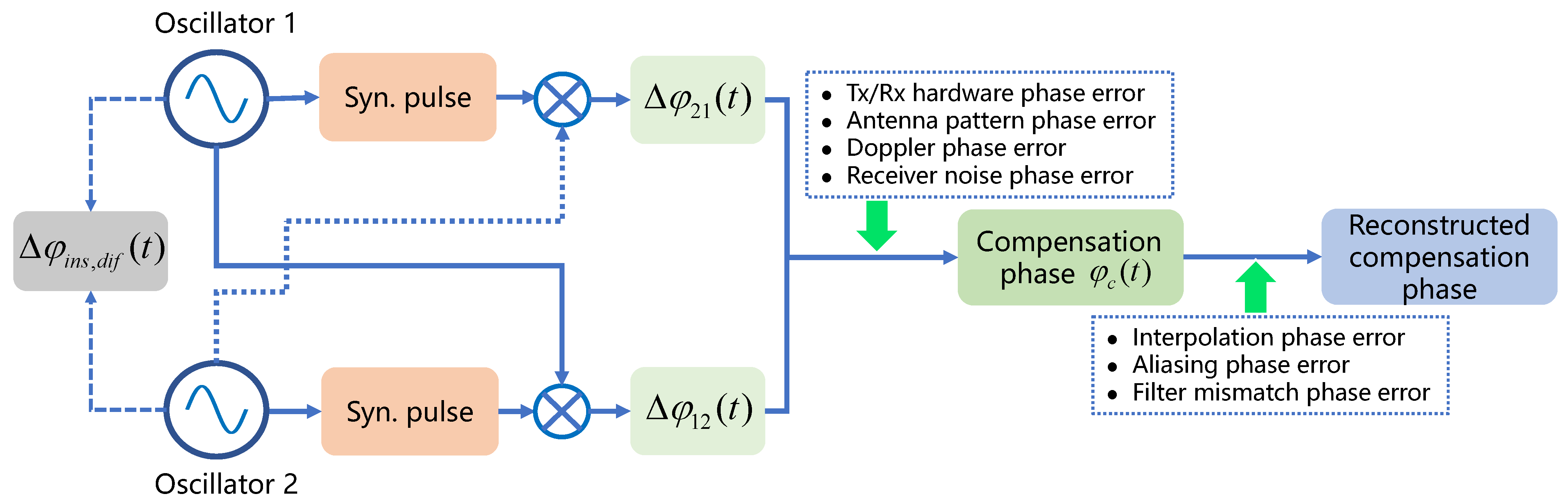
In this subsection, the error in phase synchronization is analyzed. There are two steps to obtain the final compensation phase, as shown in Figure 1. The first step is obtain the compensation phase ${\phi }_c\left(t\right)$ according to Equation (11). However, the synchronization frequency $f_{syn}$ of compensation phase ${\phi }_c\left(t\right)$ may be lower than the pulse repetition frequency ($PRF$) of echoes. Therefore, in the second step, the interpolation of ${\phi }_c\left(t\right)$ is needed to obtain the reconstructed compensation phase.

In the analysis of obtaining the compensation phase ${\phi }_c\left(t\right)$, the pulse link error is not included. However, in practice, the Tx/Rx hardware phase error, synchronization antenna pattern phase error and receiver noise phase error will also introduce other phase errors to the synchronization signal. As mentioned in [6], the advantage of using the phase difference to derive the compensation phase ${\phi }_c\left(t\right)$ is actually the difference of the difference, since the phases ${\phi }_{21}\left(t\right)$ and ${\phi }_{12}\left(t\right)$ already represent a phase difference and contain the Tx/Rx hardware and synchronization antenna pattern phase variations, which will cancel out as long as their contributions do not change within the time ${\tau }_{sys}$ [6,35]. The receiver noise which consists of thermal noise and the noise collected by synchronization antenna is the main factor that influences the accuracy of phase synchronization. In the second step of processing, not only will the components of $S_{\varphi }\left(f\right)$ outside the range $-\frac{1}{2}{f}_{syn}\sim \frac{1}{2}{f}_{syn}$ cause interpolation phase error ${\sigma }_i$, but also they will cause aliasing phase error ${\sigma }_a$ [6]. In addition, a filter mismatch phase error ${\sigma }_f$ caused by the transfer function $H_{syn}$ may appear [6]. The following is a theoretical analysis of the synchronization link. The total phase error variance is given by [6]:

$${\sigma }_{link}^2=\frac{1}{2}{\sigma }_{SNR}^2+{\sigma }_i^2+{\sigma }_a^2+{\sigma }_f^2$$

(12)

The first term in Equation (12) represents receiver noise phase error. The detailed analysis of interpolation error, aliasing error and filter mismatch error can be seen in [6]. Here, we only give a detailed description of the receiver noise phase error since it is the main error in the proposed synchronization scheme.

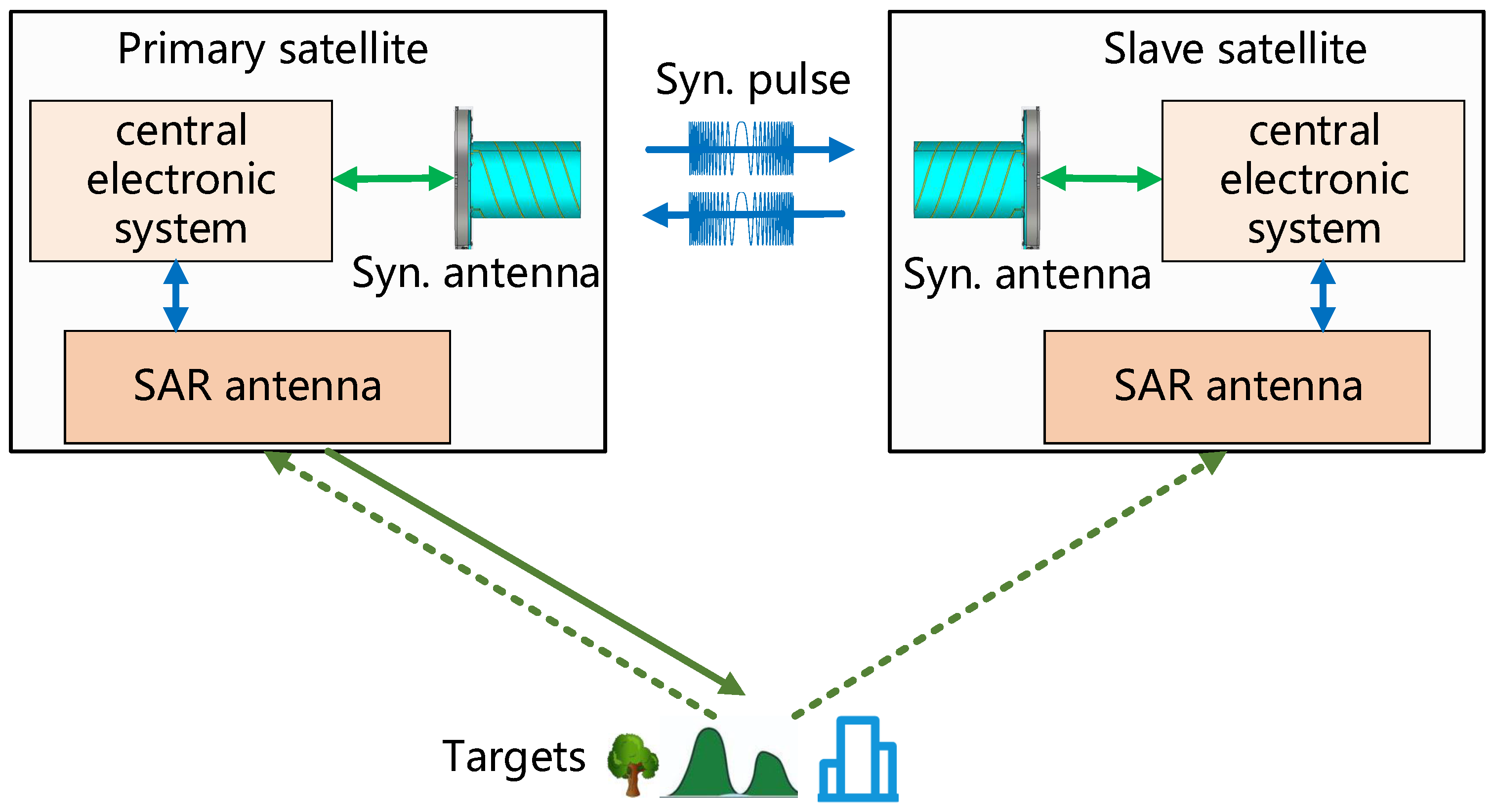
As Figure 2 shows, the synchronization signals are exchanged between the two satellites. The synchronization phase is obtained after pulse compression. After pulse compression, a phase value with high SNR will be extracted in the peak position. The accuracy of the synchronization link with different SNRs should be evaluated. The synchronization signal energy from the transmitting antenna to the receiving synchronization antenna can be calculated as [36]

$$E=\frac{P_t{G}_1{G}_2{\lambda }^2}{{\left(4\pi R\right)}^2}$$

(13)

where $P_t$ is the transmitting power, $G_1$ is the gain of the transmitting antenna, $G_2$ is the gain of the receiving antenna, and R is the distance between the two synchronization antennas. The SNR of synchronization signal after pulse compression can be written as

$$\mathrm{SNR}=\frac{E}{k_{0}B{T}_0}B{T}_{syn}=\frac{P_t{G}_1{G}_2{\lambda }^2{T}_{syn}}{k_0{T}_0{\left(4\pi R\right)}^2}$$

(14)

where B is the bandwidth of the transmitting pulse, $T_{syn}$ is the synchronization signal pulse width, $k_0$ is Boltzmann’s constant, and $T_0$ is the temperature of receiver.

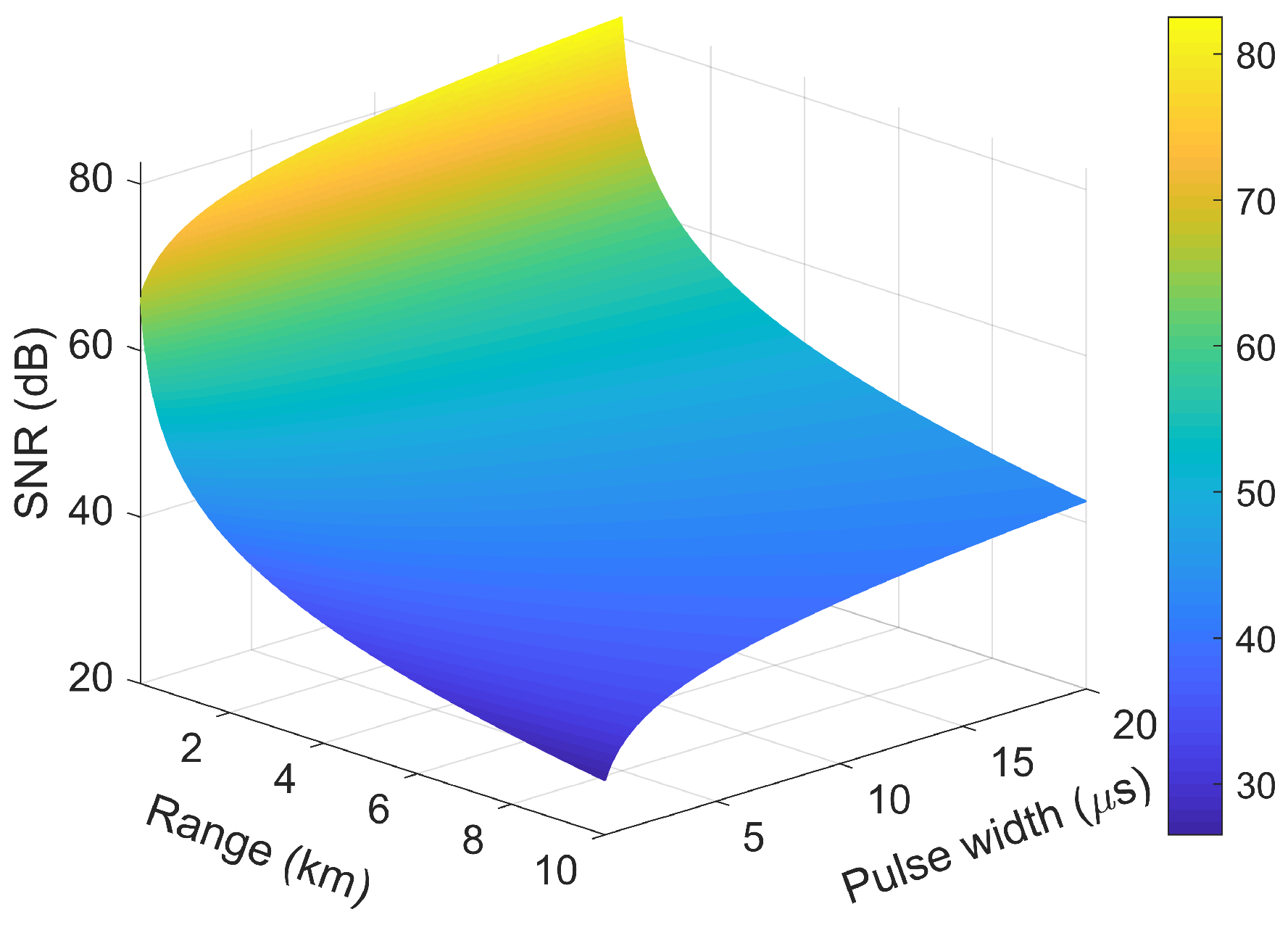
In order to achieve omnidirectional coverage, each satellite is equipped with several synchronization antennas. For example, six horn antennas are used in TanDEM-X mission [3] and four quadrifilar antennas are used in LuTan-1 mission [25]. The simulation parameters in

Table 1. The parameters used for synchronization simulation experiment.

Parameter	Symbol	Value
Syn. antenna transmitting gain	$G_1$	0 dB
Syn. antenna receiving gain	$G_2$	0 dB
Boltzmann’s constant	$k_0$	1.38 $\times {10}^{-23}$ J/K
Receiver temperature	$T_0$	300 K
Distance	R	0.1∼10 km
Synchronization signal pulse width	$T_{syn}$	0.5∼20 $\mathsf{\mu }$s

are used to present change of SNR of synchronization signal with respect to distance and pulse width. The simulation result can be seen Figure 3. The SNR decreases with the increase of the distance and the decrease of the pulse width. In the worse case of simulation, the SNR of synchronization will less than 30 dB.

The receiver noise phase error is represented by a spectral density function. For band-limited Gaussian white noise, the spectral density function is related to the SNR through [6]

$$S_{{\phi }_{\mathrm{SNR}}}\left(f\right)=\frac{1}{2f_{syn}\mathrm{SNR}}$$

(15)

The complete expression of the receiver noise is shown as follows [6]

$$\frac{1}{2}{\sigma }_{\mathrm{SNR}}^2=\frac{1}{4f_{syn}\mathrm{SNR}}\underset{-f_{syn}/2}{\overset{f_{syn}/2}{\int }}{\left|H_{syn}\left(f\right)H_{az}\left(f\right)\right|}^{2}df$$

(16)

where $H_{az}$ is the azimuth compression transfer function.

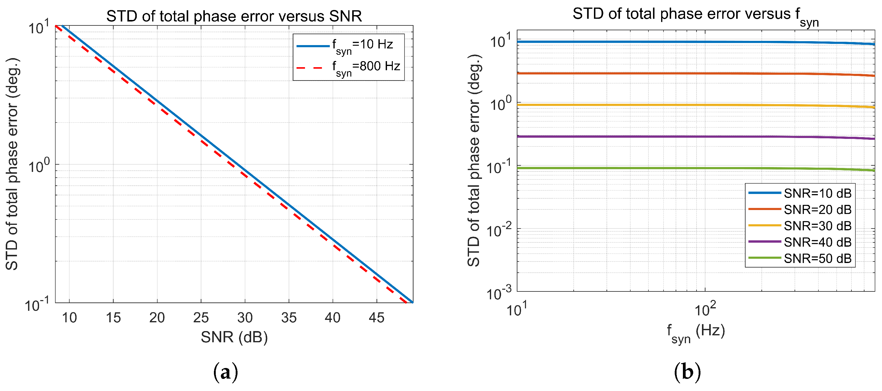
When the synchronization frequency is low, ${\sigma }_i$ and ${\sigma }_a$ are relatively large and they account for the majority of the total phase error [6]. However, when the synchronization frequency is larger than 10 Hz, ${\sigma }_i$ and ${\sigma }_a$ are relatively small and the receiver noise phase error dominates the total phase error. Since the synchronization frequency $f_{syn}$ in the proposed synchronization scheme can reach half of $PRF$, the interpolation error and aliasing error are negligible in the analysis [6]. In the case of different synchronization frequency, the standard deviation (STD) of total phase error ${\sigma }_{link}$ versus SNR is shown in Figure 4a. In the case of different SNR, ${\sigma }_{link}$ versus synchronization frequency is shown in Figure 4b. It can be seen from the simulation results that $f_{syn}$ has little impact on the STD of phase errors in the high synchronization frequency case. The STD of total phase error ${\sigma }_{link}$ is mainly depends on SNR of synchronization signal. If ${\sigma }_{link}$ is limited to no more than 1 degree, the SNR of synchronization signal should reach 30 dB at least.

2.4. Advanced Synchronization Scheme

In this subsection, an advanced synchronization scheme based on coherent integration and waveform diversity is presented. First, the timing diagram of the proposed scheme is introduced. Then, the waveform diversity technique is used to for separating the synchronization signal and echoes. Finally, the coherent integration is used to improve the SNR of synchronization signal, which can improve the accuracy of the synchronization phase. The processing of the received signal is also described in detail.

2.4.1. Timing Diagram

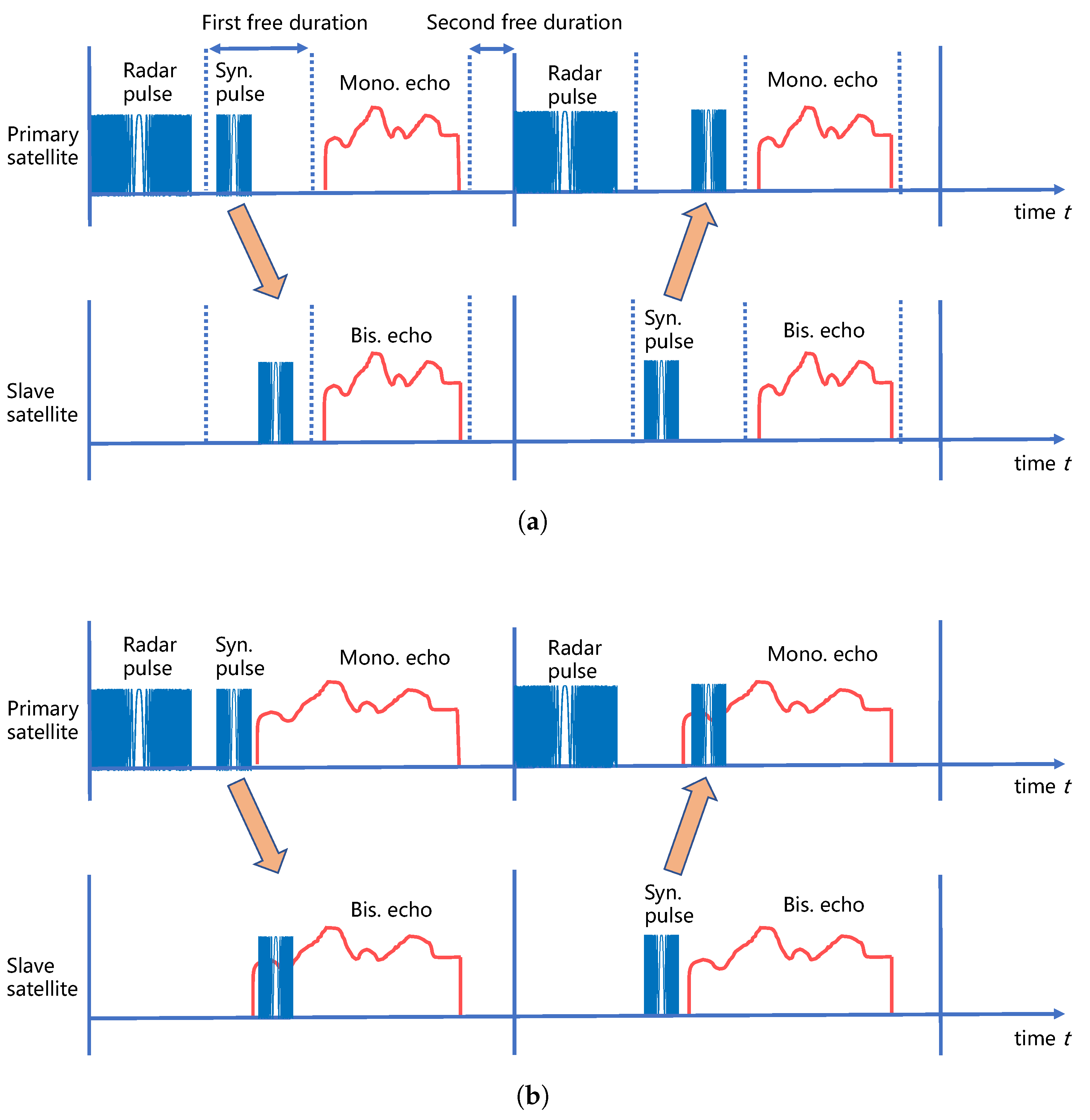
The timing diagram of the synchronization pulse exchange is shown in Figure 5. There are two free durations for the transmission of synchronization signals. The first free duration is the free duration between the ending time of the radar signal and the starting time of radar echo receiving windows, and correspondingly the second free duration is the free duration between the ending time of the radar echo receiving windows and the starting time of the next PRT. In the previous work, the phase synchronization signals are exchanged in the first free duration, which can be seen in Figure 5a [23]. Thus, the normal work of radar can be prevented from being interrupted, which can significantly improve synchronization frequency and avoid the missing data effect.

Suppose the pulse width of radar signal is $T_{radar}$, the echo receiving window length is $T_{echo}$, the following two inequality equations should be satisfied

$$\begin{array}{c}\hfill T_{radar}+T_{syn}+{\tau }_{12}+T_{echo}<PRT\end{array}$$

(17)

$$\begin{array}{c}\hfill T_{radar}+T_{syn}+{\tau }_{21}+T_{echo}<PRT\end{array}$$

(18)

It should be noted that the nadir echo receiving window should also be considered in the beam design. Here we only give a simplified discussion. The detailed analysis of beam design can be seen in [37]. Therefore, due to the extra time for transmission and receiving of synchronization signal, it may cause the decrease of echo receiving window length $T_{echo}$, which could lead to the decrease of swath coverage. In order to solve this problem, an improved timing diagram is designed which can be seen in Figure 5b. The echoes and synchronization signal are received simultaneously. In this condition, the only $T_{syn}$ occupies the PRT. As a result, the design of echo receiving window length $T_{echo}$ can have a better flexibility.

2.4.2. Waveform Diversity

After timing diagram design, the following question is how to separate the echoes and synchronization signal from the recorded data. If the radar signal and the synchronization signal use the same signal, it is difficult to separate them. A direct idea originated from the nadir echo removal [32] is using orthogonal waveforms. Two orthogonal signals are designed in the BiSAR system. One is used for radar signal, other is used for synchronization signal. The echoes and synchronization signal are received simultaneously. Then, based on waveform diversity technique, the radar signal and synchronization signal are separated, which are used for imaging processing and extracting the synchronization phase, respectively. While keeping the waveform diversity concept, the proposed technique in [32] allows removing the synchronization through a dedicated dual-focus postprocessing technique, which exploits the synchronization signal’s sparsity in range-compressed data. The detailed discussion about the dual-focus postprocessing technique can be seen in the following discussion.

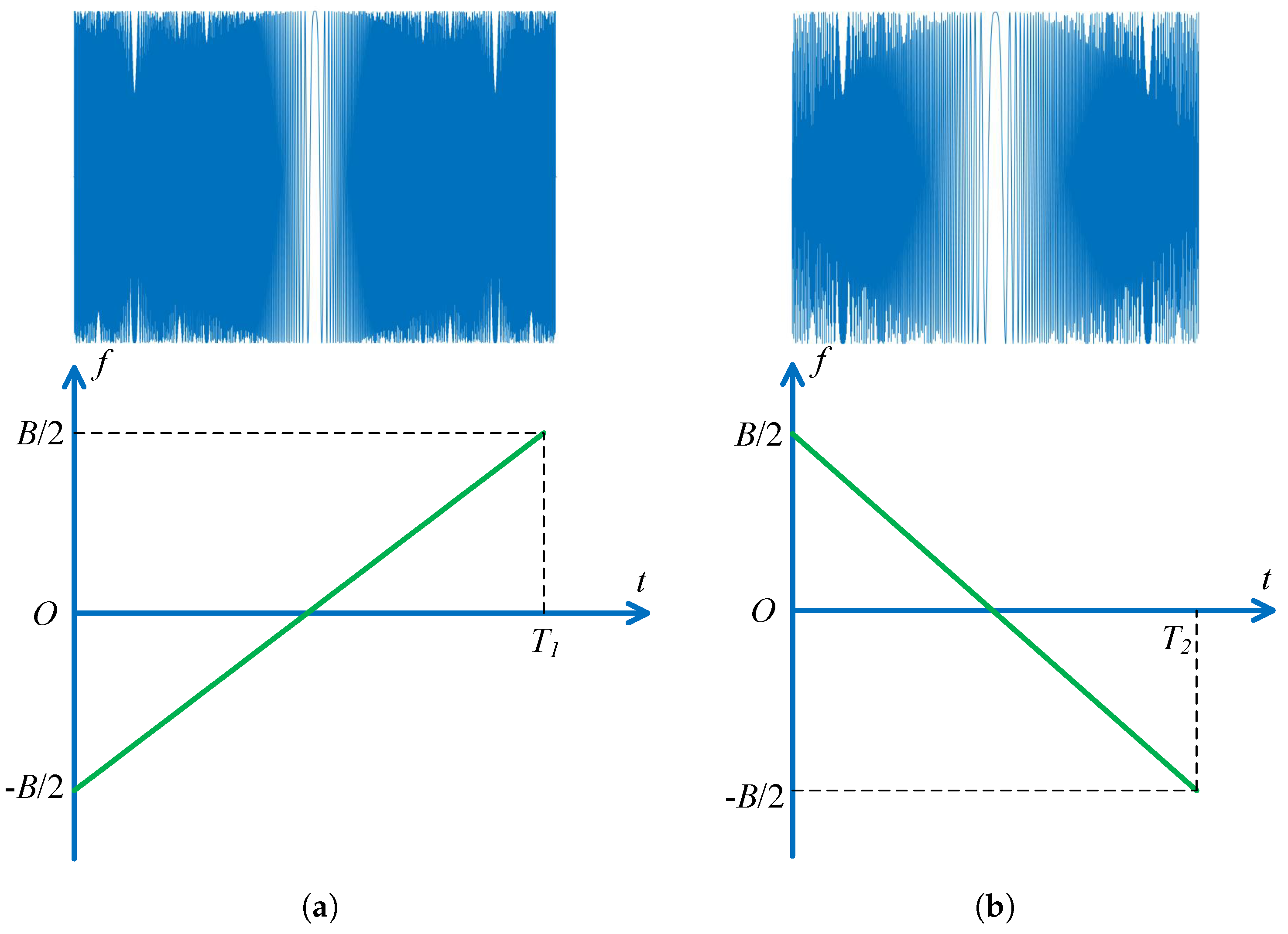
Here, a design example is illustrated. The design example is using the up and down chirps. The up and down chirps were already proposed for the suppression of range ambiguities [30]. Up and down chirps are typical examples of orthogonal waveforms. The up chirp can be represent as

$$s_1\left(t\right)=\left\{\begin{array}{c}j\pi K_1{t}^2,-\frac{T_1}{2}\le t\le \frac{T_1}{2}\hfill \\ 0,otherwise\hfill \end{array}\right.$$

(19)

where B is the bandwidth, $K_1=B/T_1$ is the frequency modulation (FM) rate of up chirp, $T_1$ is the up chirp width. The down chirp can be represent as

$$s_2\left(t\right)=\left\{\begin{array}{c}j\pi K_2{t}^2,-\frac{T_2}{2}\le t\le \frac{T_2}{2}\hfill \\ 0otherwise\hfill \end{array}\right.$$

(20)

where $K_2=-B/T_2$ is the FM rate of down chirp, $T_2$ is the down chirp width. Figure 6 schematically shows the up and down chirps. In the proposed synchronization scheme, the radar signal can be up chirp while the synchronization signal is down chirp. Also, the radar signal can be down chirp while the synchronization is up chirp.

For the received signal, one of the core problems is separating the echoes and synchronization signal. On the one hand, the echoes can be regarded as noise for synchronization signal. On the other hand, the synchronization signal is the interference for echoes, which means that the signal energy from synchronization signal is present as noise in the focused SAR image [31]. Suppose that the average power of echoes is $P_{echo}$, the thermal noise power is $P_{noise}$, and the average power of synchronization signal is $P_{syn}$. Therefore, the SNR of synchronization signal in the received signal can be expressed as

$${\mathrm{SNR}}_{data}=\frac{P_{syn}}{P_{echo}+P_{noise}}$$

(21)

After pulse compression for synchronization signal, the synchronization signal will be compressed and the peak power in peak position can be written as

$$P_{syn,com}=P_{syn}BT$$

(22)

In this case, the SNR of synchronization signal in the received signal can be expressed as

$${\mathrm{SNR}}_{data,com}=\frac{P_{syn}BT}{P_{echo}+P_{noise}}$$

(23)

However, the SNR is still low, which may not satisfy the requirement. In order to obtain a high accuracy synchronization accuracy, the coherent integration is used to improve the SNR of synchronization signal, which can be seen in the next subsection.

2.4.3. Coherent Integration

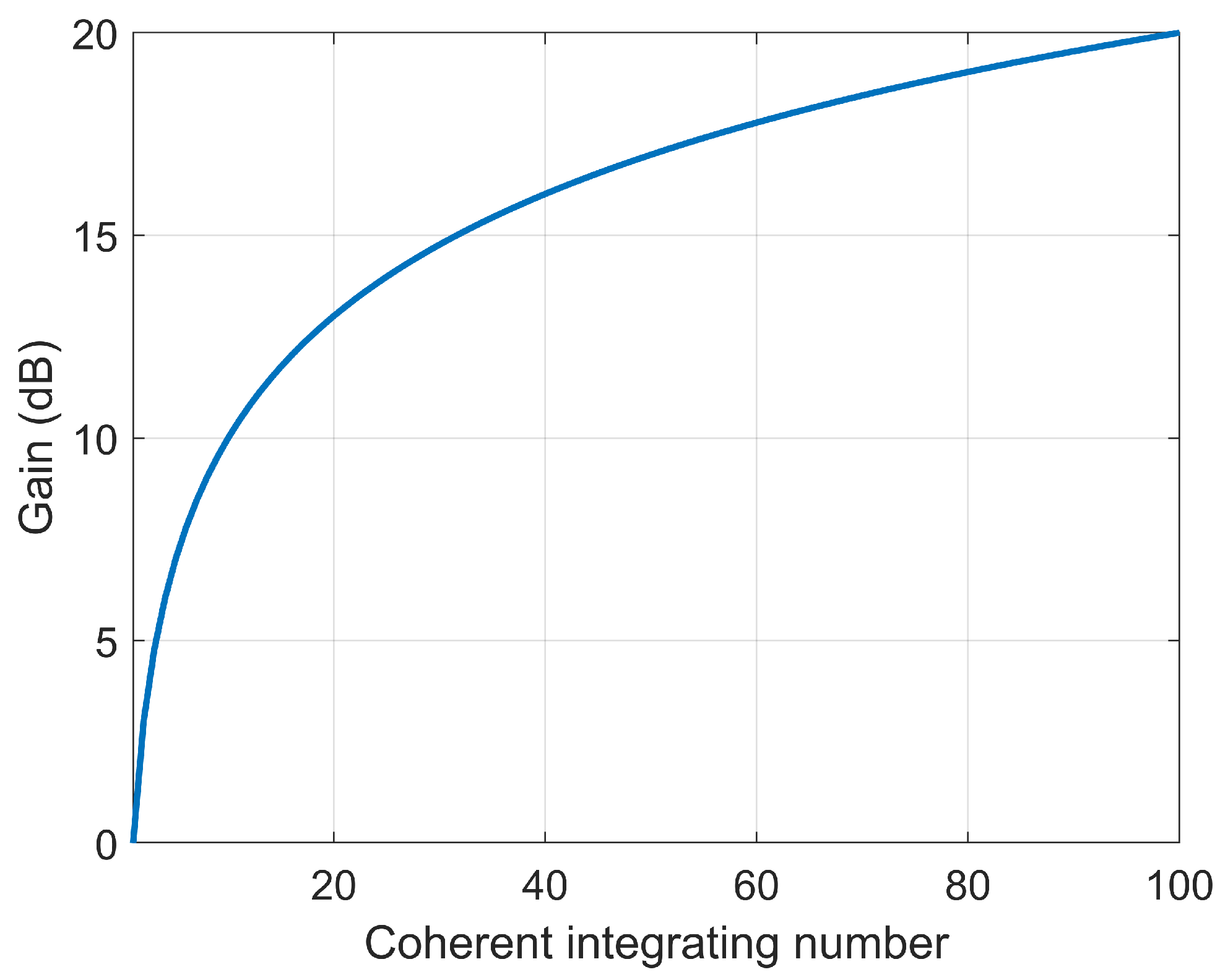
As Figure 7 shows, in coherent integration, when a perfect integrator is used, to integrate L pulses the SNR is improved by the factor $10{log}_{10}L$. Otherwise, integration loss occurs, which is always the case for non-coherent integration [38]. Coherent integration loss occurs when the integration process is not optimum. Here, we derive the coherent gain of synchronization gain in the processing of synchronization signal.

The peak signal in the peak position of synchronization pulse after pulse compression can be written as

$$s\left(t_k\right)=Aexp\left(j2\pi \Delta f_{t_k}{t}_k\right)+n\left(t_k\right)$$

(24)

where A is the amplitude, $t_k=\frac{k}{f_{syn}}=k{t}_{syn}$ is the discrete sample instances, k is the number of synchronization pulse, $\Delta f_{t_k}=\Delta f+\frac{\partial \Delta \phi \left(t\right)}{\partial t}{|}_{t=t_k}$, and $n\left(t_k\right)$ is the noise for compressed synchronization pulse in time $t_k$. It should be noted that the SAR echoes are also regraded as noise for the synchronization signal. The SNR of $s\left(t_k\right)$ can be expressed as

$${\mathrm{SNR}}_{data,com}=\frac{A^2}{{\sigma }^2}=\frac{P_{syn}BT}{P_{echo}+P_{noise}}$$

(25)

where ${\sigma }^2$ is the sum of echoes’ power and noise power.

Taking M numbers signal before and after time $t_{k_0}$, the total average number is $L=2M+1$. Therefore, the signal after average can be written as

$$\begin{array}{cc}\hfill s_L\left(t_{k_0}\right)& =\frac{1}{L}\sum _{i=-M}^{M}s\left(t_k\right)\hfill \\ \hfill & =\frac{1}{L}\sum _{i=-M}^M\left(Aexp\left(j2\pi \Delta f_{t_{k_0+i}}{t}_{k_0+i}\right)+n\left(t_{k_0+i}\right)\right)\hfill \end{array}$$

(26)

In the first step analysis, the following approximation is used, $\Delta f_{t_{k_0+i}}\approx \Delta f_{t_{k_0}}$, $i=-M,\cdots ,M$. In this case, Equation (26) can be derived as

$$s_L\left(t_{k_0}\right)=\frac{1}{L}s\left(t_{k_0}\right)G+\frac{1}{L}\sum _{i=-M}^{M}n\left(t_{k_0+i}\right)$$

(27)

where G can be expressed as

$$G=exp(-j2\pi \Delta f_{t_{k_0}}{t}_{syn}M)\frac{1-exp(j2\pi \Delta f_{t_{k_0}}{t}_{syn}L)}{1-exp(j2\pi \Delta f_{t_{k_0}}{t}_{syn})}$$

(28)

The amplitude of G is

$$\left|G\right|=\left|\frac{sin(2\pi \Delta f_{t_{k_0}}{t}_{syn}L)}{sin(2\pi \Delta f\left(t_{k_0}\right)t_{syn})}\right|$$

(29)

If $2\pi \Delta f_{t_{k_0}}{t}_{syn}L$ is small enough, $\left|G\right|\approx L$. Hence, the SNR of signal after L times average can be expressed as

$${\mathrm{SNR}}_{data,com,L}=\frac{A^2{L}^2}{L{\sigma }^2}=\frac{A^{2}L}{{\sigma }^2}=L·{\mathrm{SNR}}_{data,com}$$

(30)

However, the analysis above is not practical in the case of L is large and the approximation $\Delta f_{t_{k_0\pm M}}\approx \Delta f_{t_{k_0}}$ is no longer applicable. Coherent integration can not be applied over a large number of pulses, particularly when frequency offset is varying rapidly. In general, if the coherent integrating number L is not very large, the SNR of synchronization can be improved accordingly. For example, if we average 10 pulses, coherent gain of SNR is about 10 dB, which can improve the accuracy of synchronization phase.

2.5. Processing Flowchart

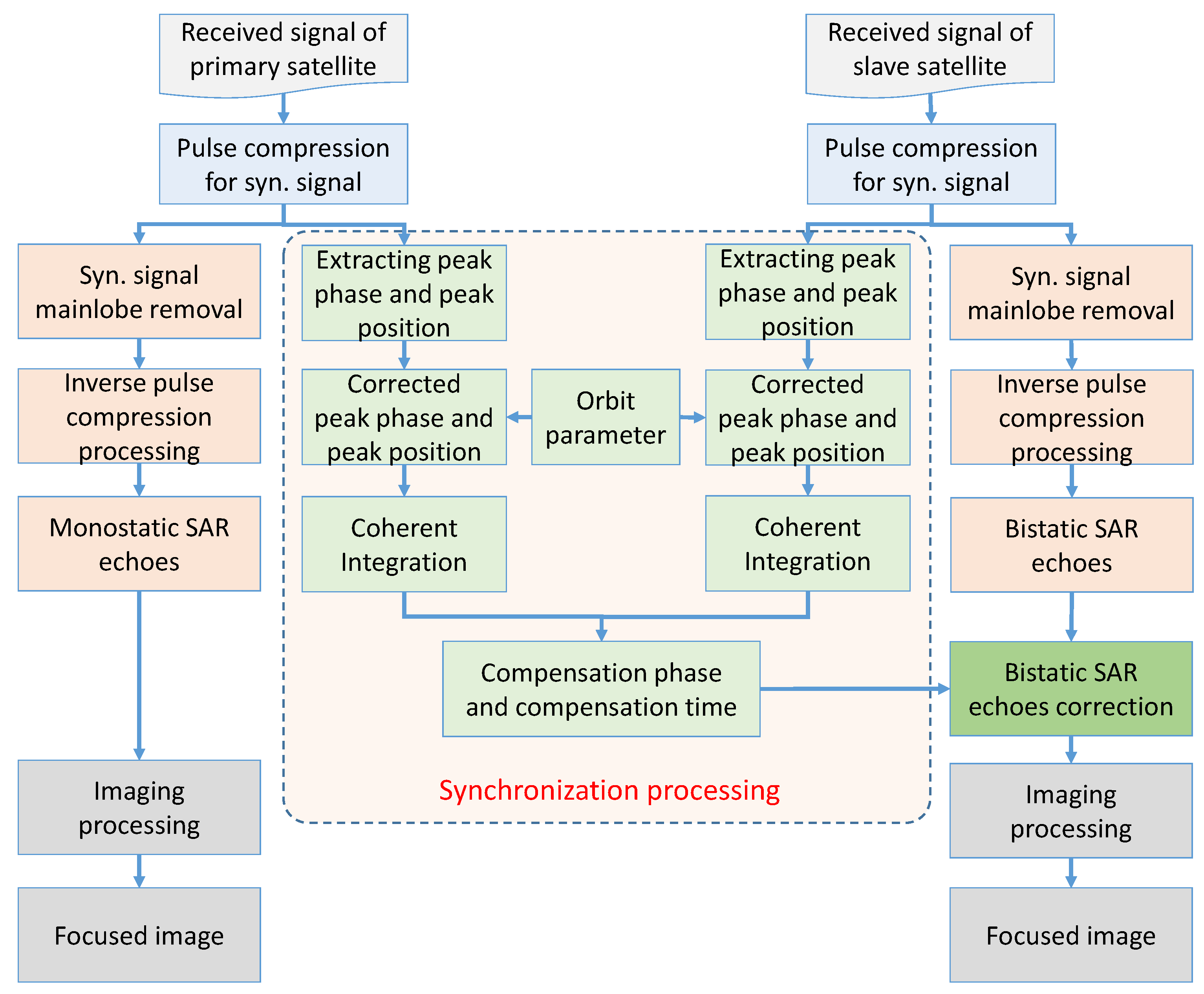
In this subsection, the processing flowchart of the proposed synchronization scheme, as shown in Figure 8, is presented. First, the processing for extracting the synchronization signal is introduced. Then dual-focus postprocessing technique for removing the synchronization signal is described in detail.

2.5.1. Processing for Extracting the Synchronization Signal

The processing for extracting the synchronization signal in received signal can be summarized as follows:

step1 

Pulse compression for synchronization signal. The received signal is compressed using a filter “matched” to the synchronization signal.

step2 

Extract peak phase and peak position.

step3 

Correction by orbit parameters. The Doppler effect and relativistic effect should be corrected according to the orbit parameters.

step4 

Coherent Integration. The coherent integration technique is used to improve the SNR of synchronization signal.

step5 

Obtain compensation phase and compensation time. The compensation time can be obtained by compensation phase and corrected peak position.

step6 

Compensation for bistatic SAR echoes.

It should be noted that in step3, the relativistic effect should also be corrected, which has been discussed in [39]. In addition, in step5, the detailed processing to obtain the compensation time can be seen in [35] in detail.

2.5.2. Processing for Extracting the Echoes

If the synchronization signal is not eliminated in the received signal, the SAR image after imaging focusing will have low SNR, which degrades the quality of SAR image. This reason is immediately evident based on Parseval’s theorem [31]. According to Parseval’s theorem, the output signals of all focusing filters will hence have the same power regardless of whether a matched or an unmatched signal is present. This means that the signal energy from synchronization signal is still present in the final focused image.

The dual-focus postprocessing, which has been proposed for removing the nadir echo signal in [32], is used to remove the synchronization signal for the received signal. While keeping the waveform diversity concept, the synchronization signal can be removed by a dedicated dual-focus postprocessing, which exploits the synchronization signal’s sparsity in range-compressed data. The processing steps can be summarized as follows:

step1 

Pulse compression for synchronization signal. The received signal is compressed using a filter “matched” to the synchronization signal.

step2 

Remove the synchronization signal. The synchronization signal can be removed by blanking the pixels where there is the mainlobe of compressed synchronization signal.

step3 

Inverse pulse compression processing. The data is processed by the inverse filter “matched” to the synchronization signal. After that, the data is transformed back into raw data, which can be regarded as the SAR echoes.

step4 

Synchronization compensation. The compensation phase and compensation time is compensated for the BiSAR echoes.

step5 

Imaging processing. The final image can be obtained after imaging processing.

The core of the processing is the waveform diversity concept. The received signal are first compressed using a filter “matched” to the synchronization signal, so that the synchronization signal can be removed with a negligible corruption of the echo signal, as the synchronization signal is compressed and located at specific range bins, while the echoes are smeared [32]. Through an inverse pulse compressed operation, the received data, in which the synchronization signal has been significantly attenuated, is transformed back into raw data, while can be regarded as the the echoes that is only minimally affected.

3. Results

In this section, the simulation experiments are performed to demonstrate the effectiveness of the proposed scheme. First, the STD of total phase error ${\sigma }_{link}$ versus coherent integration number is presented. Then, the echoes of distributed targets are simulated to show the processing step of the proposed scheme.

3.1. Oscillator Phase Error Simulation

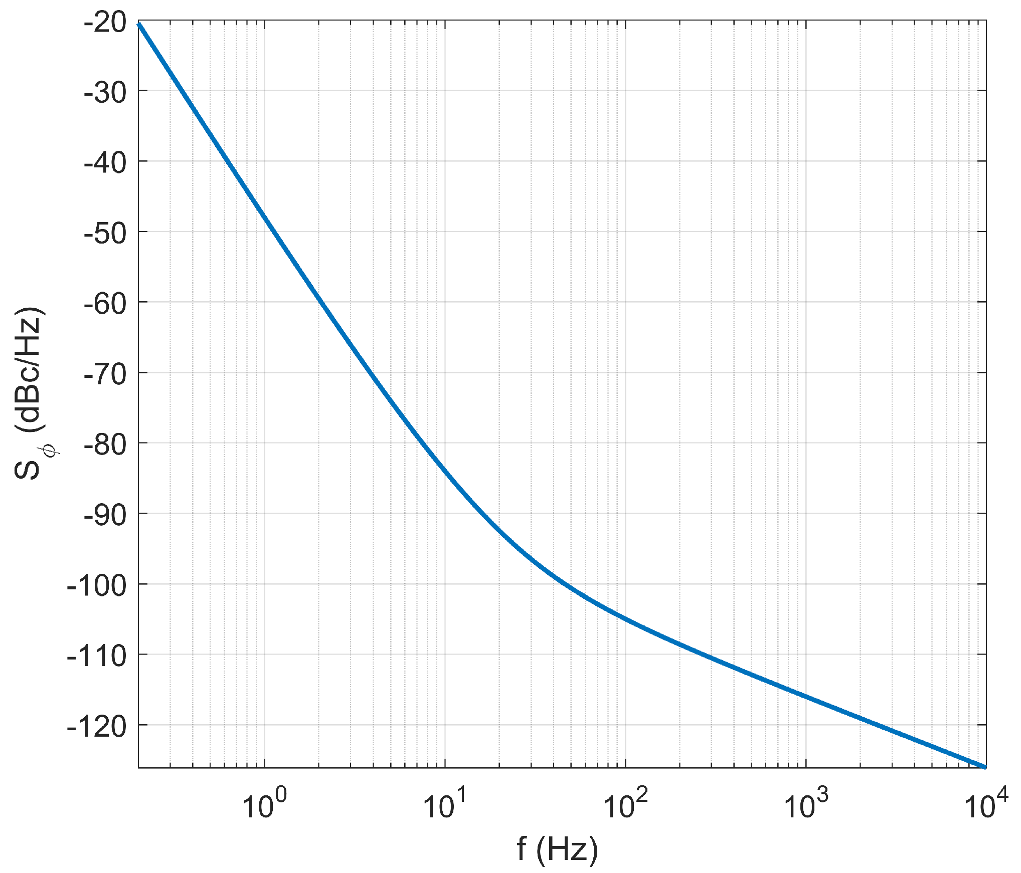
As mentioned above, the power spectral density $S_{\varphi }\left(f\right)$ describes a random process of stationary term $\Delta {\varphi }_{st}\left(t\right)$. Figure 9 shows as an example of a typical phase spectrum $S_{\varphi }\left(f\right)$ of a oscillator. The phase noise level of the oscillator versus specific frequency is given in

Table 2. Example of Single Sideband Phase Noise Levels, Given in dBc/Hz.

Frequency	1 Hz	10 Hz	${10}^2$ Hz	${10}^3$ Hz	${10}^4$ Hz
Phase noise level	−48	−84	−105	−116	−124

. Then the digital model for power law noises proposed in [40] is used for generating digital sequences of oscillator phase error. $S_{\varphi }\left(f\right)$ is used for simulation and the oscillator phase error for a time interval of 500 s is obtained. The simulation results can be seen in Figure 10.

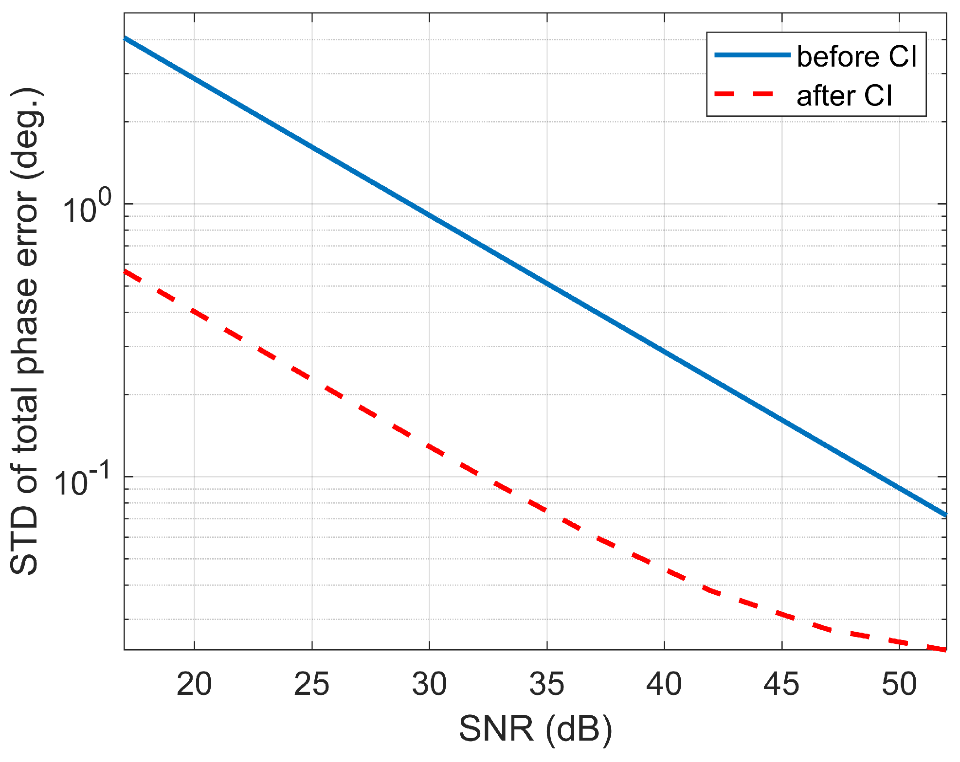
The synchronization signals under different SNRs are simulated. The synchronization frequency is 143 Hz and the average number L is 51. Therefore, the corresponding average time is 0.3566 s. The SNR gain is $10{log}_{10}L=17$ dB. The simulation results can be seen in Figure 11. From the simulation result we can seen that the STD of phase errors is reduced after coherent integration.

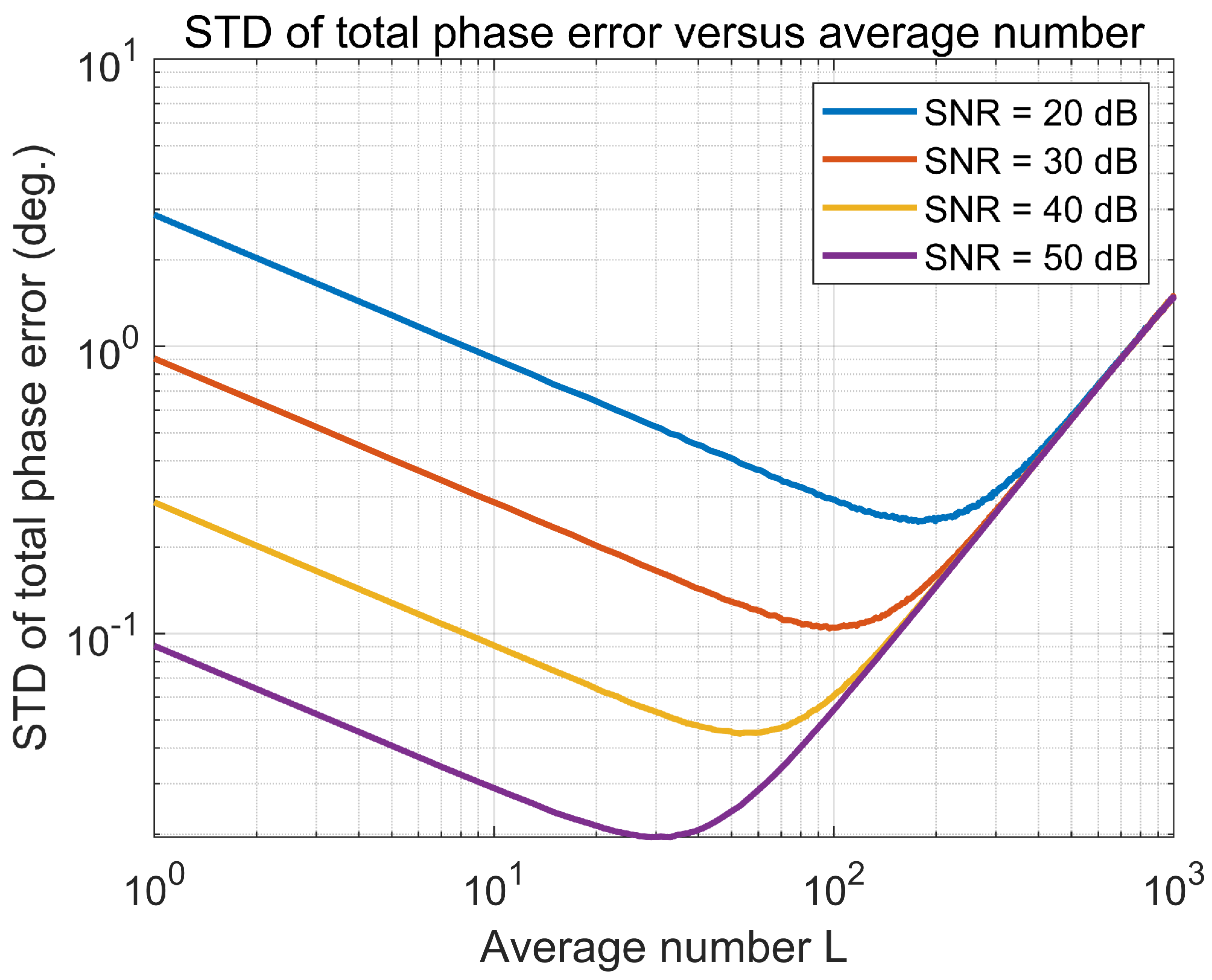
The influence of different average number is also simulated and result can be seen in Figure 12. The STD of phase errors first decreases with the increase of average number L and then increases with the increase of L. The reasons can be summarized as follows. If the signals are coherent, the ${\mathrm{SNR}}_{data,com,L}$ will increase with the increase of L, resulting in a high accuracy synchronization phase. However, when the signals are not coherent, the accuracy will decrease. Therefore, there is a compromise between the coherence and average number. From the simulation result, we can seen that the average number should be chosen carefully.

3.2. Distributed Targets Simulation

The distributed targets simulation experiment is performed to verify the effectiveness of the proposed algorithm. A real monostatic SAR complex imagery with 0.9 m range resolution and 0.4 m azimuth resolution is acquired by Gaofen-3 satellite in the spotlight mode [41]. The scattering coefficient of this imagery is used for simulating the echoes. The simulation parameters can be seen in

Table 3. Parameters in Distributed Targets Simulation.

Parameter	Value
Carrier frequency	1.26 GHz
Orbit height	600 km
Incidence angle	30${}^{\circ }$
Radar signal bandwidth	80 MHz
Radar signal pulse width	60 $\mathsf{\mu }$s
Radar signal FM rate	$1.333\times {10}^{12}$ Hz/s
Synchronization signal bandwidth	80 MHz
Synchronization signal pulse width	20 $\mathsf{\mu }$s
Synchronization signal FM rate	$-4\times {10}^{12}$ Hz/s
Sampling frequency	90 MHz
PRF	1898 Hz
Doppler bandwidth	1400 Hz

. The radar signal is up chirp while the synchronization signal is down chirp. The radar signal and synchronization signal have the same bandwidth 80 MHz. The primary satellite transmits the synchronization signal after transmitting the radar signal, then, the primary satellite receives the echoes from the ground while the slave satellite receives the echoes and synchronization signal simultaneously. In the next PRT, the primary satellite transmits the radar signal, then the slave satellite transmits the synchronization signal to the primary satellite. After that, the primary satellite receives the echoes and synchronization signal simultaneously while the slave satellite only receives the echoes. It should be noted that, if the synchronization signal arrives before echoes, a delay line can be used for delaying the arriving time of the synchronization signal [42].

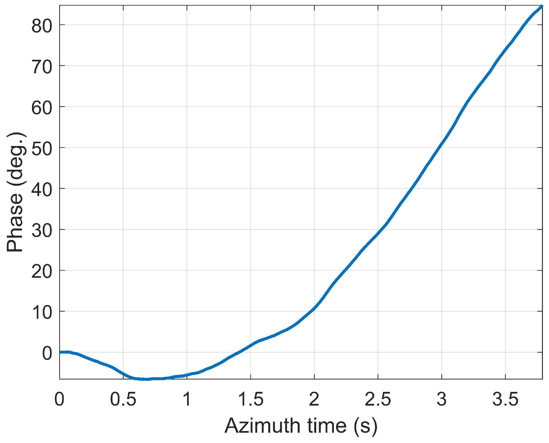
The synchronization error used in simulation can be seen in Figure 13. The simulated received signal, which contains the echoes and synchronization signal can be seen in Figure 14a. In the simulation, the synchronization frequency is half of PRF. Therefore, not all received signal contains the synchronization signal. In the first PRT, received signal of slave satellite contains the synchronization signal. In the next PRT, received signal of primary satellite contains the synchronization signal. Only half of the received signal contains the synchronization signal. In the simulation, the synchronization signal power $P_{syn}$ is half of the sum of echoes power $P_{echo}$ and noise power $P_{noise}$, $P_{syn}=(P_{echo}+P_{noise})/2$. Therefore, the SNR of synchronization signal in received signal is ${\mathrm{SNR}}_{data}=10{log}_{10}(P_{syn}/(P_{echo}+P_{noise}))=-3$ dB.

3.2.1. Extracting Synchronization Phase

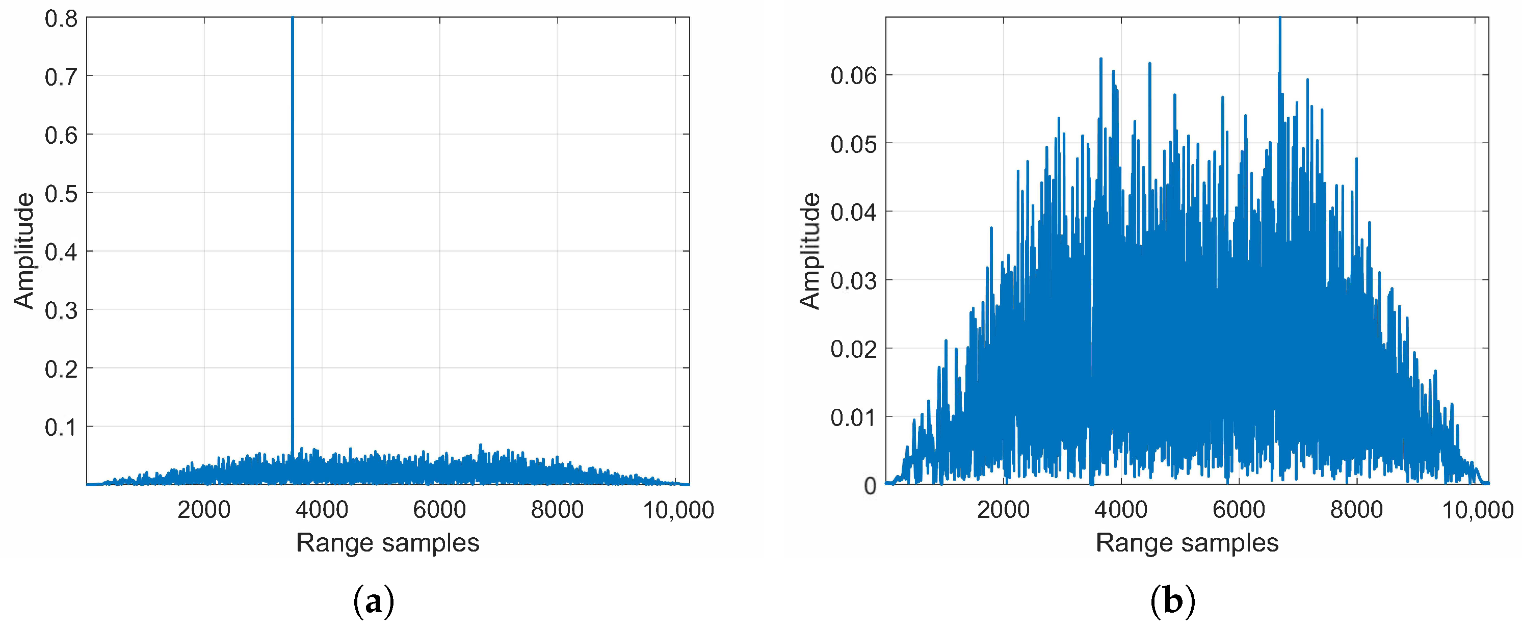
The received signal contains the synchronization signal and echoes. In order to extract the synchronization phase, the first step of the processing is pulse compression for synchronization signal. After pulse compression, the result can be seen in Figure 14b. Figure 15a depicts the signal in a range line corresponding to Figure 14b. The SNR of the synchronization signal after pulse compression is ${\mathrm{SNR}}_{data,com}=29$ dB. This is based on the fact that the compression gain is $10{log}_{10}\left(B_r{T}_{syn}\right)$ = 32 dB. Before pulse compression, the SNR of synchronization signal is ${\mathrm{SNR}}_{data}=-3$ dB. Therefore, ${\mathrm{SNR}}_{data,com}={\mathrm{SNR}}_{data}+10{log}_{10}\left(B_r{T}_{syn}\right)=29$ dB. The SNR of synchronization signal is in agreement with the theoretical analysis.

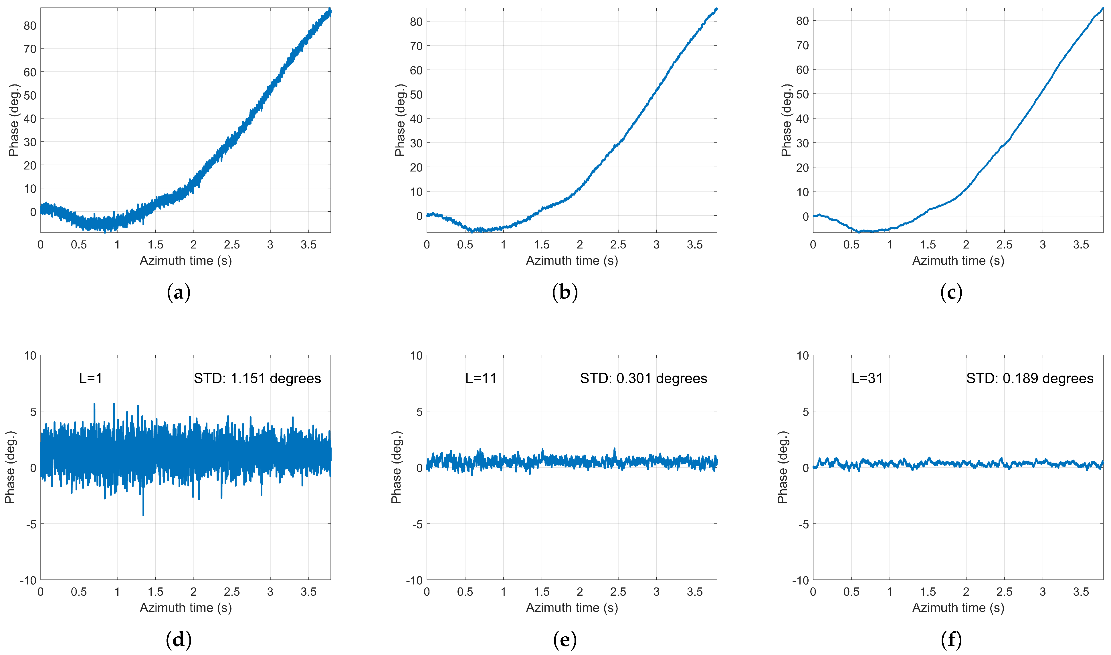
The next step is coherent integration. Here, the average number L = 1, 11, 32 are processed respectively. The results can be seen in Figure 16. As shown Figure 16, before coherent integration, the STD of phase errors is 1.151 degrees. However, after 11 averages, the STD of phase errors is 0.301 degrees. After 31 averages, the STD of phase errors is less than 0.2 degrees, which proves the effectiveness of the proposed synchronization scheme.

3.2.2. Extracting Echo Signal

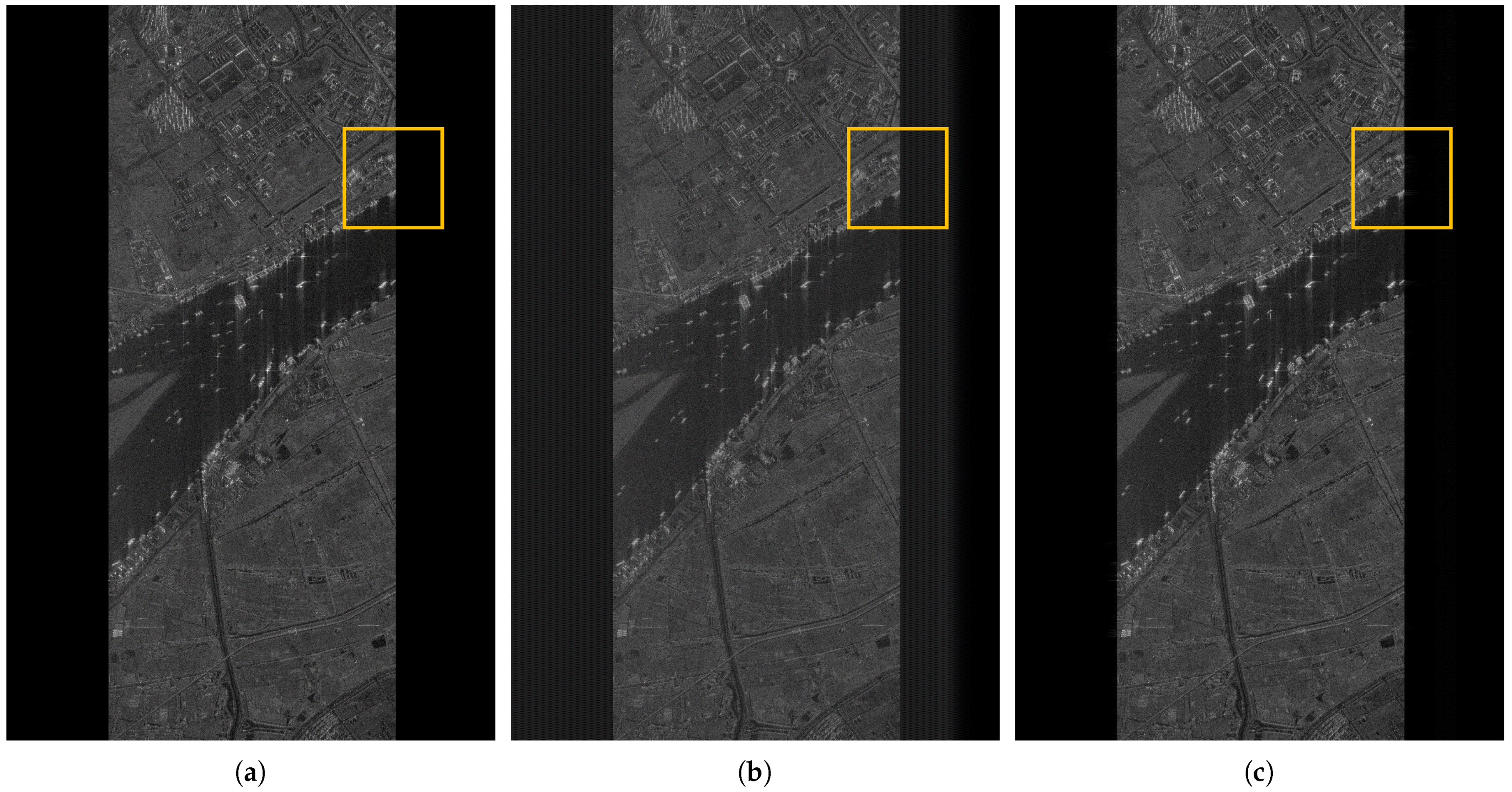
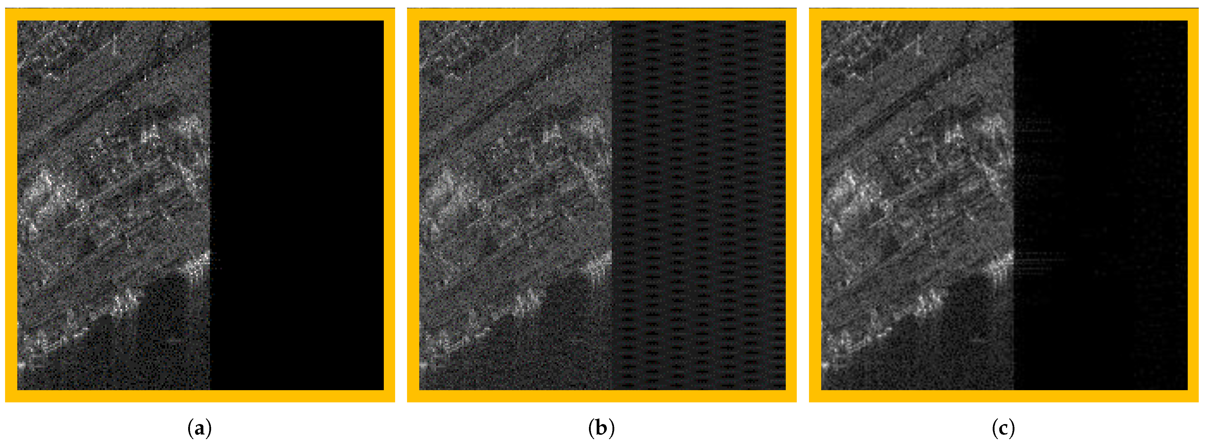
After pulse compression for synchronization signal, the synchronization signal is compressed in the peak position. Therefore, the following step is blanking the pixels where there is the mainlobe of the compressed synchronization signal. The processing result can be seen in Figure 14c. At this time, the synchronization signal is removed in the received signal, only the echoes are left. The following step is inverse pulse compression processing. At this point, the data is transformed into the time domain and the echoes are obtained, which can be seen in Figure 14d. A range line in Figure 14d after removing synchronization signal and inverse pulse compression processing is shown in Figure 15b. Then, the BiSAR echoes are compensated by compensation phase and compensation time. The omega-K algorithm is used for imaging processing [43]. After processing with imaging algorithm, the imaging result can be seen in Figure 17c. In order to compare the imaging result without the removal of synchronization signal, the imaging result (also after synchronization phase compensation) can be seen in Figure 17b. Figure 17a is the reference imaging result (the received signal only contains the echoes in simulation). For comparison, the imaging result of local area in Figure 17 is shown in Figure 18. It can be seen that, if the synchronization signal is not removed, the imaging results will have higher noise and the quality of the image will decrease. However, after synchronization signal removal, the imaging result will have a good quality which is almost same with the reference image. The results prove that the dual-focus postprocessing is effective in the processing of the received signal.

4. Conclusions

In the BiSAR system, any deviation between two oscillators in different platforms will cause a modulation of BiSAR echo. Therefore, phase synchronization is one of the key issues that must be addressed for the BiSAR system. An advanced phase synchronization scheme is proposed for the BiSAR system, which has the advantage of high accuracy synchronization without effect on swath coverage. The synchronization signal and radar signal are orthogonal signals which can be separated by using waveform diversity technique. In addition, the phase synchronization accuracy can be further improved by coherent integration. The transmission of synchronization signals between two synchronization antennas is analyzed, followed by the theoretical error analysis. Then, the simulation experiments are conducted. The simulation experiment is in accordance with the theoretical analysis. Based on waveform diversity technique, the separation of synchronization signal and echoes is feasible. The results show that the proposed synchronization scheme has a high synchronization accuracy.

In the distributed targets simulation, the synchronization signal power $P_{syn}$ is half of the sum of echoes power $P_{echo}$ and noise power $P_{noise}$, Therefore, the SNR of synchronization signal in received signal is ${\mathrm{SNR}}_{data}=-3$ dB. After coherent integration, the SNR of synchronization signal can reach 29 dB, therefore, the results show high accuracy. However, in reality, the SNR of synchronization signal in received signal may be much less than −3 dB. As a result, the SNR of synchronization signal after coherent integration may be small, which can not guarantee the accuracy. In addition, there are some other challenging factors that need further consideration: The power of the received signal that contains the synchronization signal and echoes in specific range bins is larger than the received signal that only contains the echoes, which may influence the block adaptive quantization compression for the received signal; While the synchronization antenna receives the synchronization signal, it may also receive the echoes, which may cause the ambiguities in the final image since the echoes received by synchronization antenna have different echo delay compared with the echoes received by the SAR antenna; In turn, while the SAR antenna receives the echoes, it may also receive the synchronization signal, which may cause the ambiguities of the synchronization signal. In the future, we will conduct further research on the problems mentioned above.

References

- Moreira, A.; Prats-Iraola, P.; Younis, M.; Krieger, G.; Hajnsek, I.; Papathanassiou, K.P. A Tutorial On Synthetic Aperture Radar. IEEE Geosci. Remote Sens. Mag. 2013, 1, 6–43. [Google Scholar] [CrossRef] [Green Version]
- Duque, S.; López-Dekker, P.; Mallorqui, J.J. Single-pass bistatic SAR interferometry using fixed-receiver configurations: Theory and experimental validation. IEEE Trans. Geosci. Remote Sens. 2010, 48, 2740–2749. [Google Scholar] [CrossRef]
- Krieger, G.; Moreira, A.; Fiedler, H.; Hajnsek, I.; Werner, M.; Younis, M.; Zink, M. TanDEM-X: A Satellite Formation for High-Resolution SAR Interferometry. IEEE Trans. Geosci. Remote Sens. 2007, 45, 3317–3341. [Google Scholar] [CrossRef] [Green Version]
- Krieger, G.; Moreira, A. Spaceborne bi- and multistatic SAR: Potential and challenges. IEEE Proc. Radar Sonar Navig. 2006, 153, 184–198. [Google Scholar] [CrossRef] [Green Version]
- Eineder, M. Ocillator clock drift compensation in bistatic interferometric SAR. In Proceedings of the IGARSS 2013—2003 IEEE International Geoscience and Remote Sensing Symposium, Toulouse, France, 21–25 July 2003; Volume 3, pp. 1449–1451. [Google Scholar]
- Younis, M.; Metzig, R.; Krieger, G. Performance prediction of a phase synchronization link for bistatic SAR. IEEE Geosci. Remote Sens. Lett. 2006, 3, 429–433. [Google Scholar] [CrossRef] [Green Version]
- Krieger, G.; Younis, M. Impact of oscillator noise in bistatic and multistatic SAR. IEEE Geosci. Remote Sens. Lett. 2006, 3, 424–428. [Google Scholar] [CrossRef] [Green Version]
- Krieger, G. Advanced bistatic and multistatic SAR concepts and applications. In Proceedings of the EUSAR 2006—6th European Synthetic Aperture Radar Conference Tutorial, Dresden, Germany, 16–18 May 2006; pp. 1–100. [Google Scholar]
- Ludlow, A.D.; Zelevinsky, T.; Campbell, G.; Blatt, S.; Boyd, M.; de Miranda, M.H.; Martin, M.; Thomsen, J.; Foreman, S.M.; Ye, J.; et al. Sr lattice clock at 1 × 10⁻¹⁶ fractional uncertainty by remote optical evaluation with a Ca clock. Science 2008, 319, 1805–1808. [Google Scholar] [CrossRef] [PubMed]
- Nicholson, T.; Campbell, S.; Hutson, R.; Marti, G.; Bloom, B.; McNally, R.; Zhang, W.; Barrett, M.; Safronova, M.; Strouse, G.; et al. Systematic evaluation of an atomic clock at 2 × 10⁻¹⁸ total uncertainty. Nat. Commun. 2015, 6, 1–8. [Google Scholar] [CrossRef] [PubMed]
- Nemitz, N.; Ohkubo, T.; Takamoto, M.; Ushijima, I.; Das, M.; Ohmae, N.; Katori, H. Frequency ratio of Yb and Sr clocks with 5 × 10⁻¹⁷ uncertainty at 150 seconds averaging time. Nat. Photonics 2016, 10, 258. [Google Scholar] [CrossRef]
- Lezius, M.; Wilken, T.; Deutsch, C.; Giunta, M.; Mandel, O.; Thaller, A.; Schkolnik, V.; Schiemangk, M.; Dinkelaker, A.; Kohfeldt, A.; et al. Space-borne frequency comb metrology. Optica 2016, 3, 1381–1387. [Google Scholar] [CrossRef]
- Oelker, E.; Hutson, R.; Kennedy, C.; Sonderhouse, L.; Bothwell, T.; Goban, A.; Kedar, D.; Sanner, C.; Robinson, J.; Marti, G.; et al. Demonstration of 4.8 × 10⁻¹⁷ stability at 1 s for two independent optical clocks. Nat. Photonics 2019, 13, 714–719. [Google Scholar] [CrossRef] [Green Version]
- Rodriguez-Cassola, M.; Prats-Iraola, P.; Lopez-Dekker, P.; Reigber, A.; Krieger, G.; Moreira, A. Autonomous time and phase calibration of spaceborne bistatic SAR systems. In Proceedings of the EUSAR 2014—10th European Conference on Synthetic Aperture Radar, Berlin, Germany, 3–5 June 2014; pp. 264–267. [Google Scholar]
- Lopez-Dekker, P.; Mallorqui, J.J.; Serra-Morales, P.; Sanz-Marcos, J. Phase Synchronization and Doppler Centroid Estimation in Fixed Receiver Bistatic SAR Systems. IEEE Trans. Geosci. Remote Sens. 2008, 46, 3459–3471. [Google Scholar] [CrossRef]
- Weib, M. Synchronisation of bistatic radar systems. In Proceedings of the IGARSS 2004—2004 IEEE International Geoscience and Remote Sensing Symposium, Anchorage, AK, USA, 20–24 September 2004; Volume 3, pp. 1750–1753. [Google Scholar]
- Breit, H.; Younis, M.; Balss, U.; Niedermeier, A.; Grigorov, C.; Hueso-Gonzalez, J.; Krieger, G.; Eineder, M.; Fritz, T. Bistatic synchronization and processing of TanDEM-X data. In Proceedings of the IGARSS 2011—2011 IEEE International Geoscience and Remote Sensing Symposium, Vancouver, BC, Canada, 24–29 July 2011; pp. 2424–2427. [Google Scholar]
- Weigt, M.; Grigorov, C.; Steinbrecher, U.; Schulze, D. TanDEM-X Mission: Long Term in Orbit Synchronisation Link Performance Analysis. In Proceedings of the EUSAR 2014—10th European Conference on Synthetic Aperture Radar, Berlin, Germany, 3–5 June 2014; pp. 1–4. [Google Scholar]
- Lipiński, M.; Włostowski, T.; Serrano, J.; Alvarez, P. White rabbit: A PTP application for robust sub-nanosecond synchronization. In Proceedings of the 2011 IEEE International Symposium on Precision Clock Synchronization for Measurement, Control and Communication, Munich, Germany, 12–16 September 2011; IEEE: Piscataway, NJ, USA, 2011; pp. 25–30. [Google Scholar]
- Two Way Time Transfer. Available online: https://tf.nist.gov/time/twoway.htm (accessed on 12 December 2020).
- Pinheiro, M.; Rodriguez-Cassola, M. Reconstruction Methods of Missing SAR Data: Analysis in the Frame of TanDEM-X Synchronization Link. In Proceedings of the EUSAR 2012—9th European Conference on Synthetic Aperture Radar, Nuremberg, Germany, 23–26 April 2012; pp. 742–745. [Google Scholar]
- Pinheiro, M.; Rodriguez-Cassola, M.; Prats-Iraola, P.; Reigber, A.; Krieger, G.; Moreira, A. Reconstruction of Coherent Pairs of Synthetic Aperture Radar Data Acquired in Interrupted Mode. IEEE Trans. Geosci. Remote Sens. 2015, 53, 1876–1893. [Google Scholar] [CrossRef]
- Liang, D.; Liu, K.; Yue, H.; Chen, Y.; Deng, Y.; Zhang, H.; Li, C.; Jin, G.; Wang, R. An advanced non-interrupted synchronization scheme for bistatic synthetic aperture radar. In Proceedings of the IGARSS 2019—2019 IEEE International Geoscience and Remote Sensing Symposium, Yokohama, Japan, 28 July–2 August 2019; pp. 1116–1119. [Google Scholar]
- Liang, D.; Liu, K.; Zhang, H.; Deng, Y.; Liu, D.; Chen, Y.; Li, C.; Yue, H.; Wang, R. A High-Accuracy Synchronization Phase-Compensation Method Based on Kalman Filter for Bistatic Synthetic Aperture Radar. IEEE Geosci. Remote Sens. Lett. 2020, 17, 1722–1726. [Google Scholar] [CrossRef]
- Jin, G.; Liu, K.; Liu, D.; Liang, D.; Zhang, H.; Ou, N.; Zhang, Y.; Deng, Y.; Li, C.; Wang, R. An Advanced Phase Synchronization Scheme for LT-1. IEEE Trans. Geosci. Remote Sens. 2020, 58, 1735–1746. [Google Scholar] [CrossRef]
- Liang, D.; Liu, K.; Zhang, H.; Chen, Y.; Yue, H.; Liu, D.; Deng, Y.; Lin, H.; Fang, T.; Li, C.; et al. The Processing Framework and Experimental Verification for the Noninterrupted Synchronization Scheme of LuTan-1. IEEE Trans. Geosci. Remote Sens. 2020. [Google Scholar] [CrossRef]
- Calderbank, R.; Howard, S.D.; Moran, B. Waveform diversity in radar signal processing. IEEE Signal Process. Mag. 2009, 26, 32–41. [Google Scholar] [CrossRef]
- Gini, F.; De Maio, A.; Patton, L. Waveform Design and Diversity for Advanced Radar Systems; Institution of Engineering and Technology: London, UK, 2012. [Google Scholar]
- Zhao, P.; Deng, Y.; Wang, W.; Liu, D.; Wang, R. Azimuth Ambiguity Suppression for Hybrid Polarimetric Synthetic Aperture Radar via Waveform Diversity. Remote Sens. 2020, 12, 1226. [Google Scholar] [CrossRef] [Green Version]
- Mittermayer, J.; Martinez, J.M. Analysis of range ambiguity suppression in SAR by up and down chirp modulation for point and distributed targets. In Proceedings of the IGARSS 2003–2003 IEEE International Geoscience and Remote Sensing Symposium. Proceedings (IEEE Cat. No.03CH37477), Toulouse, France, 21–25 July 2003; Volume 6, pp. 4077–4079. [Google Scholar]
- Krieger, G. MIMO-SAR: Opportunities and Pitfalls. IEEE Trans. Geosci. Remote Sens. 2014, 52, 2628–2645. [Google Scholar] [CrossRef] [Green Version]
- Villano, M.; Krieger, G.; Moreira, A. Nadir Echo Removal in Synthetic Aperture Radar via Waveform Diversity and Dual-Focus Postprocessing. IEEE Geosci. Remote Sens. Lett. 2018, 15, 719–723. [Google Scholar] [CrossRef]
- D’Errico, M. Distributed Space Missions for Earth System Monitoring; Springer Science & Business Media: New York, NY, USA, 2012; Volume 31. [Google Scholar]
- Younis, M.; Metzig, R.; Krieger, G.; Bachmann, M.; Klein, R. Performance prediction and verification for the synchronization link of TanDEM-X. In Proceedings of the IGARSS 2007—IEEE International Geoscience and Remote Sensing Symposium, Barcelona, Spain, 23–27 July 2007; pp. 5206–5209. [Google Scholar]
- Breit, H.; Lachaise, M.; Balss, U.; Rossi, C.; Fritz, T.; Niedermeier, A. Bistatic and Interferometric Processing of TanDEM-X Data. In Proceedings of the EUSAR 2012; 9th European Conference on Synthetic Aperture Radar, Nuremberg, Germany, 23–26 April 2012; pp. 93–96. [Google Scholar]
- Balanis, C.A. Antenna Theory: Analysis and Design, 3rd ed.; Wiley-Interscience: New York, NY, USA, 2005. [Google Scholar]
- Younis, M.; Huber, S.; Patyuchenko, A.; Bordoni, F.; Krieger, G. Performance comparison of reflector-and planar-antenna based digital beam-forming SAR. Int. J. Antennas Propag. 2009, 2009. [Google Scholar] [CrossRef]
- Mahafza, B.R.; Elsherbeni, A. MATLAB Simulations for Radar Systems Design; Chapman and Hall/CRC: Boca Raton, FL, USA, 2003. [Google Scholar]
- Krieger, G.; De Zan, F. Relativistic Effects in Bistatic Synthetic Aperture Radar. IEEE Trans. Geosci. Remote Sens. 2014, 52, 1480–1488. [Google Scholar] [CrossRef]
- Kasdin, N.J. Discrete simulation of colored noise and stochastic processes and 1/fα power law noise generation. Proc. IEEE 1995, 83, 802–827. [Google Scholar] [CrossRef]
- Liang, D.; Zhang, H.; Fang, T.; Lin, H.; Liu, D.; Jia, X. A Modified Cartesian Factorized Backprojection Algorithm Integrating with Non-Start-Stop Model for High Resolution SAR Imaging. Remote Sens. 2020, 12, 3807. [Google Scholar] [CrossRef]
- Krieger, G.; Zonno, M.; Mittermayer, J.; Moreira, A.; Huber, S.; Rodriguezcassola, M. MirrorSAR: A Fractionated Space Transponder Concept for the Implementation of Low-Cost Multistatic SAR Missions. In Proceedings of the EUSAR 2018—12th European Conference on Synthetic Aperture Radar, Aachen, Germany, 4–7 June 2018; pp. 1359–1364. [Google Scholar]
- Cumming, I.G.; Wong, F.H. Digital Processing of Synthetic Aperture Radar Data: Algorithms and Implementation; Artech House: Norwood, MA, USA, 2005. [Google Scholar]
Figure 1.
The error in phase synchronization.
Figure 2.
The geometry of BiSAR system. The synchronization signals are transmitted and received by two synchronization antennas. The radar signal is transmitted by SAR antenna of primary satellite. The echoes of targets are received by two SAR antennas of primary satellite and slave satellite.
Figure 3.
The SNR varies with distance and pulse width under the condition of W.
Figure 4.
(a) The STD of total phase error versus the SNR under different synchronization frequency. (b) The STD of total phase error versus the synchronization frequency under different SNR.
Figure 5.
(a) Timing diagram of phase synchronization scheme proposed in [23]. (b) Timing diagram of proposed phase synchronization scheme.
Figure 6.
(a) Up chirp. (b) Down chirp.
Figure 7.
The coherent gain versus coherent integrating number.
Figure 8.
The processing flowchart of the proposed synchronization scheme.
Figure 9.
Power spectral density of oscillator phase noise.
Figure 10.
Simulated oscillator phase errors in 500 s data taking.
Figure 11.
The comparison of STD of total phase errors versus the SNR before coherent integration and after coherent integration. The coherent integrating number .
Figure 12.
The STD of total phase error versus average number L under different SNR conditions.
Figure 13.
The preset synchronization phase error in distributed targets simulation experiment.
Figure 14.
(a) The received signal. (b) After pulse compression for synchronization signal. (c) After the removal of the mainlobe of compressed synchronization signal. (d) After inverse pulse compression processing.
Figure 15.
(a) A range line in Figure 14b (after pulse compression for synchronization signal). (b) A range line in Figure 14d (after removing synchronization signal and inverse pulse compression processing).
Figure 16.
(a–c) The estimated synchronization phase. (d–f) The residual phase after compensation. (a,d) L = 1; (b,e) L = 11; (c,f) L = 31.
Figure 17.
The imaging result. (a) The reference image. (b) Without removal of synchronization signal. (c) After removal of synchronization signal.
Figure 18.
The local imaging area in Figure 17. (a) The reference image. (b) Without removal of synchronization signal. (c) After removal of synchronization signal.