
Signal Photon Extraction Method for Weak Beam Data of ICESat-2 Using Information Provided by Strong Beam Data in Mountainous Areas


Abstract
:
1. Introduction
2. Materials and Methods
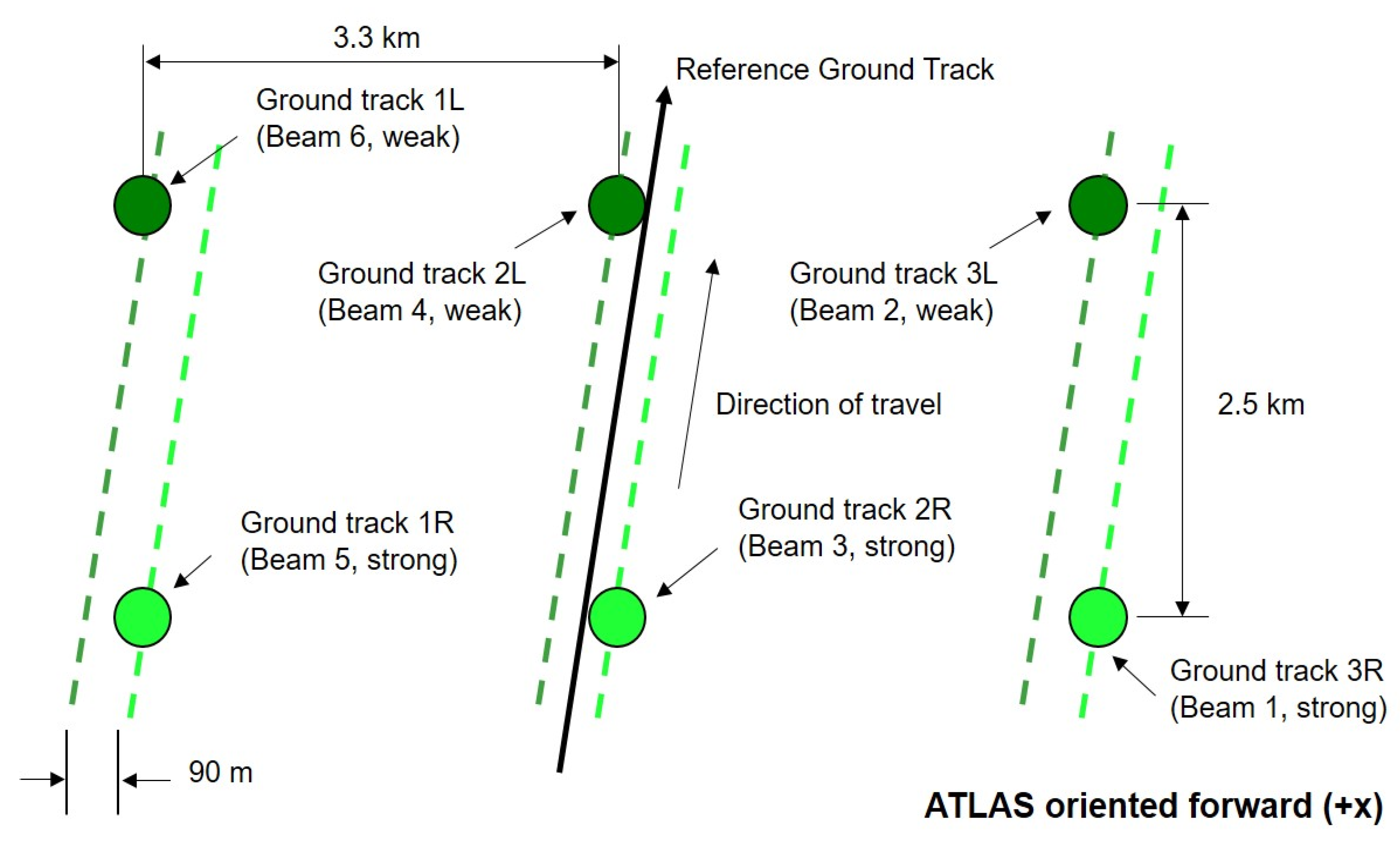
2.1. Overview of the Ice, Cloud, and land Elevation Satellite-2 (ICESat-2) Photon-Counting LiDAR
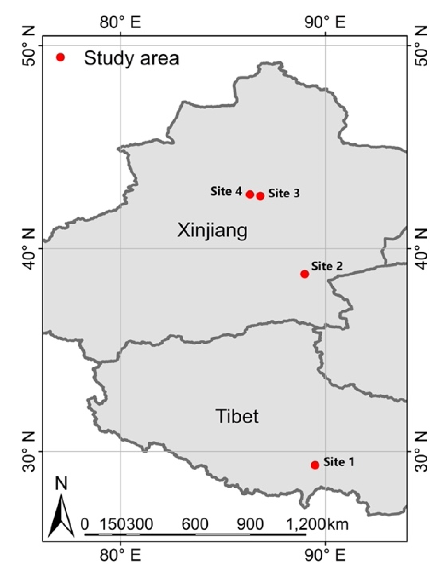
2.2. Study Areas and Datasets
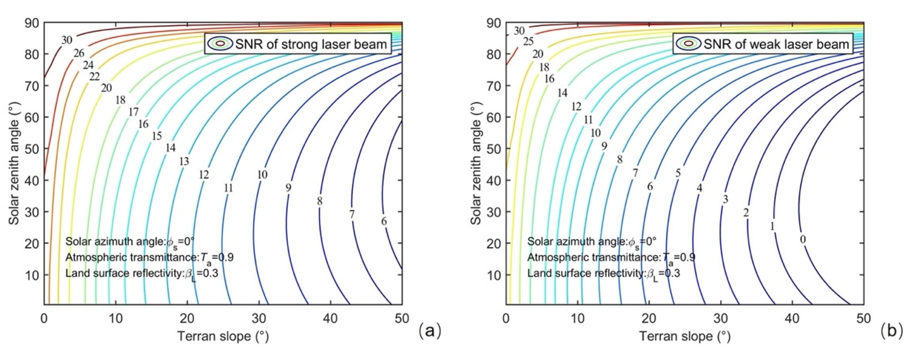
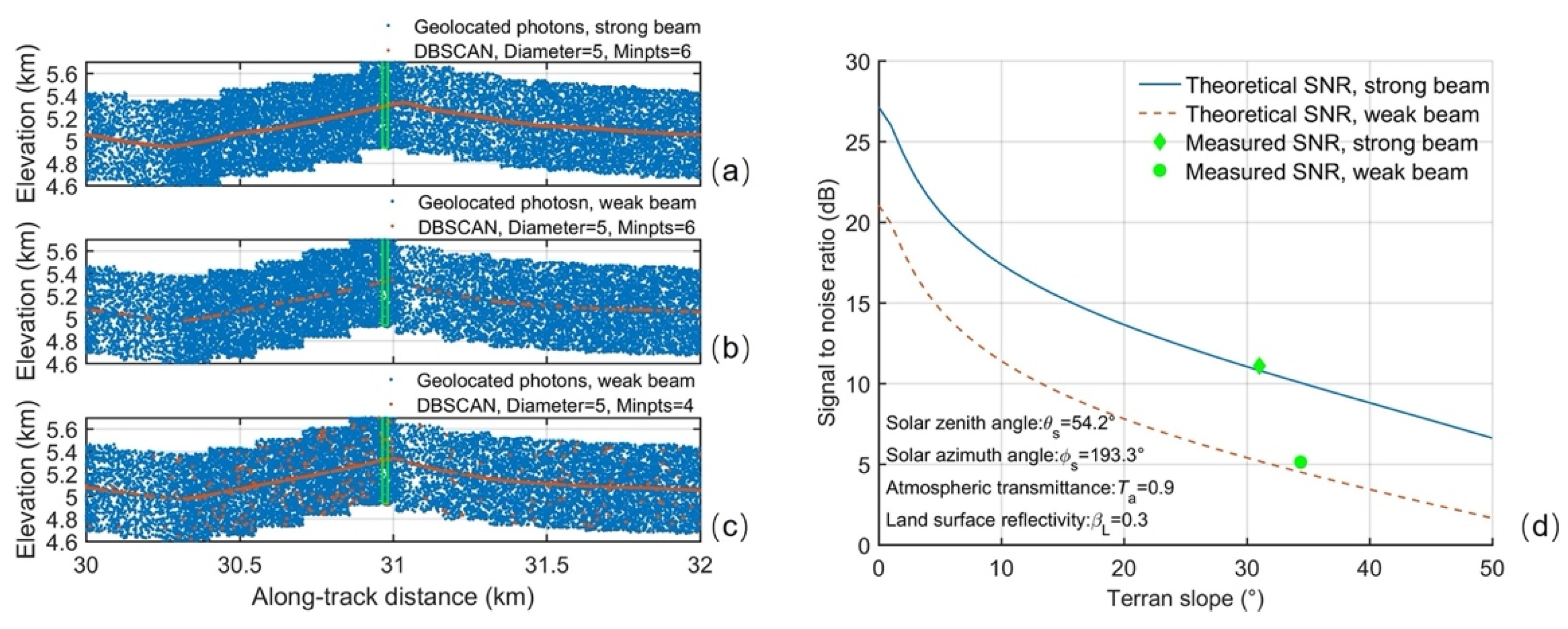
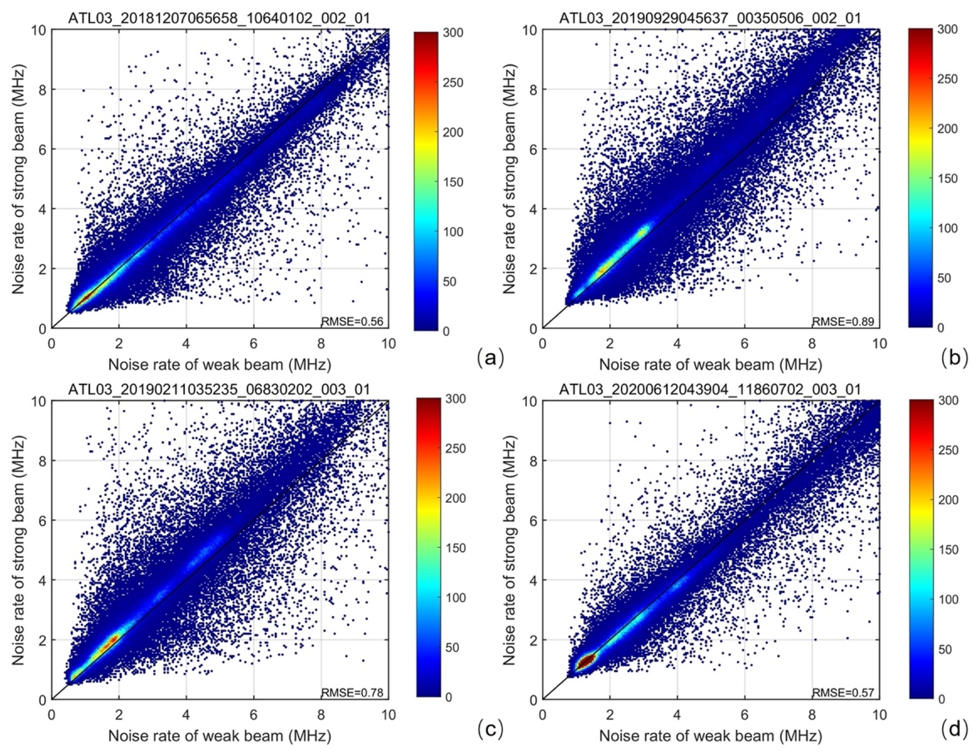
2.3. Signal–Noise Ratios (SNRs) of Different Laser Beams in Mountainous Areas
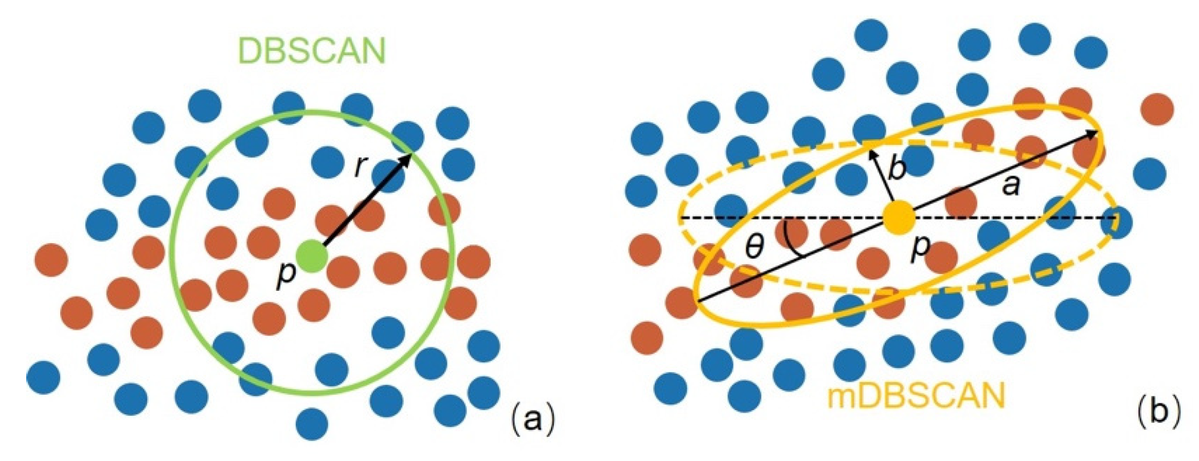
2.4. Current Density-Based Spatial Clustering of Applications with Noise (DBSCAN) Algorithm and Its Modification
2.5. Parameters Determination for Modified DBSCAN
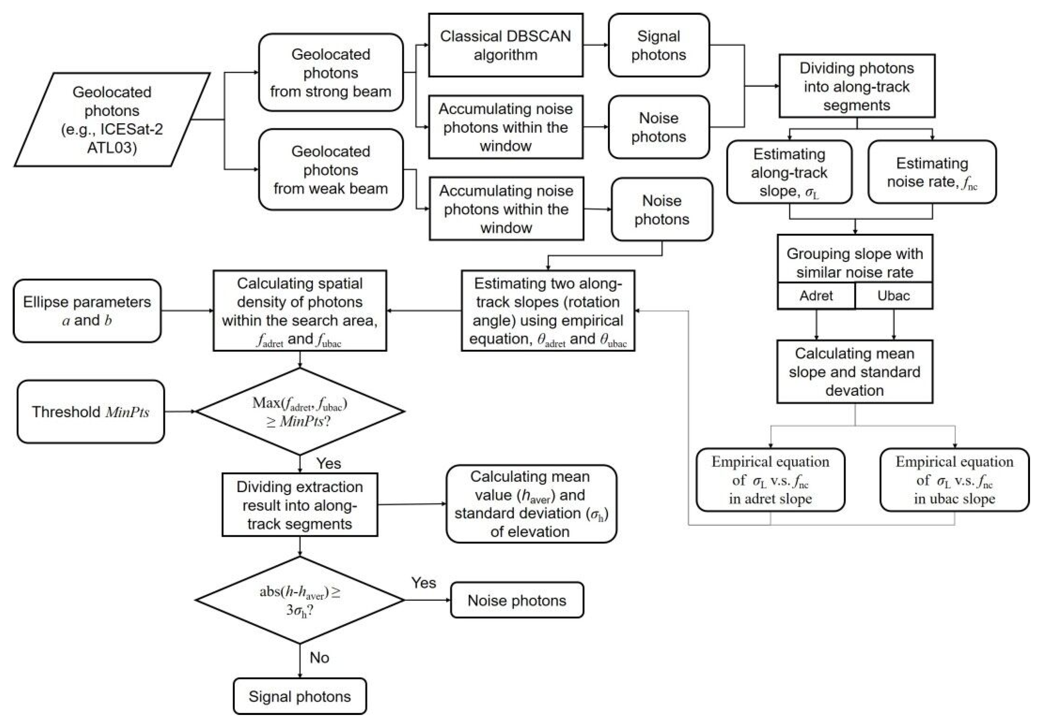
2.6. Modified DBSCAN Algorithm
- (1)
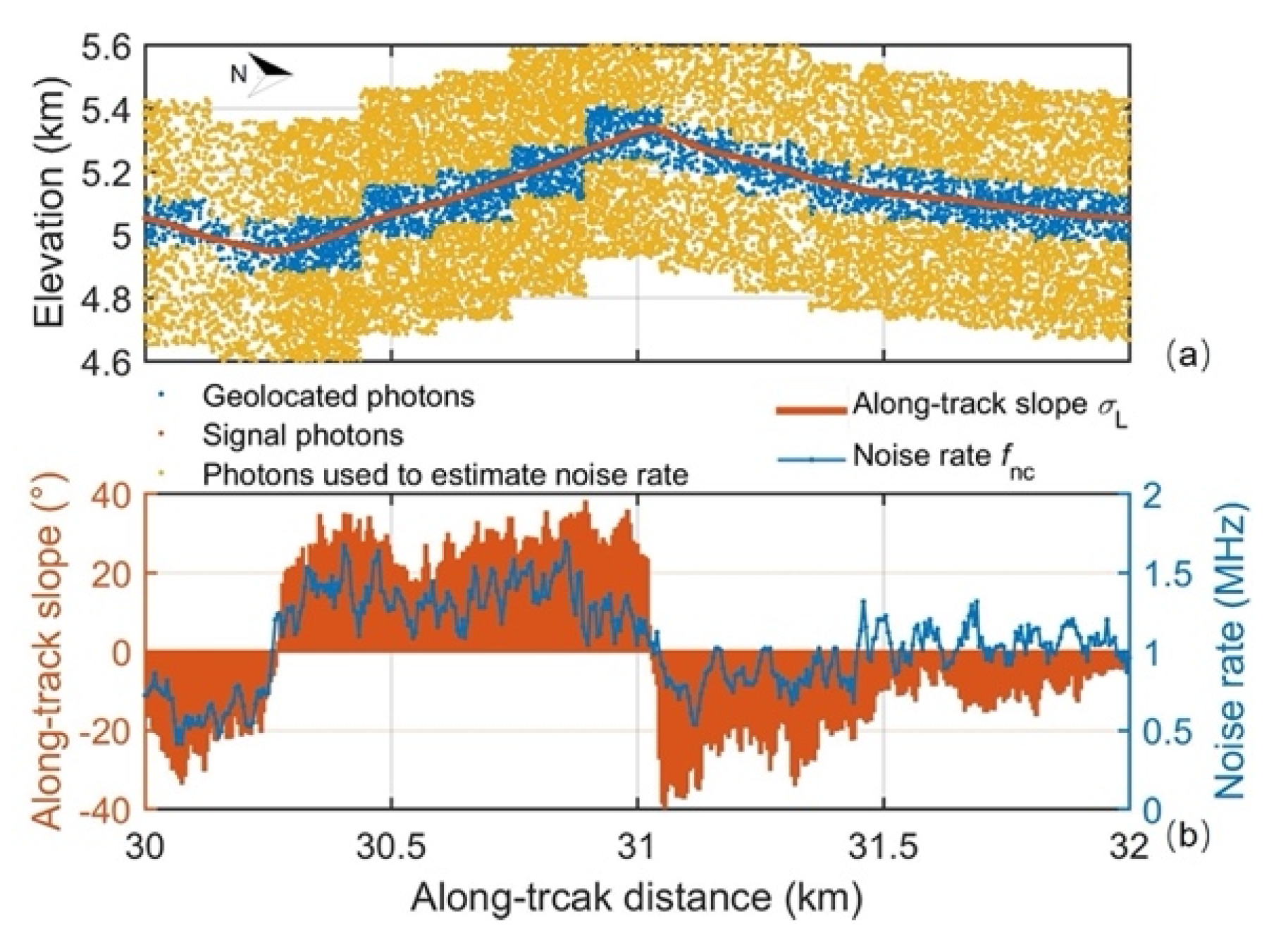
- Signal extraction and statistical parameter estimation from strong beam data
- (2)
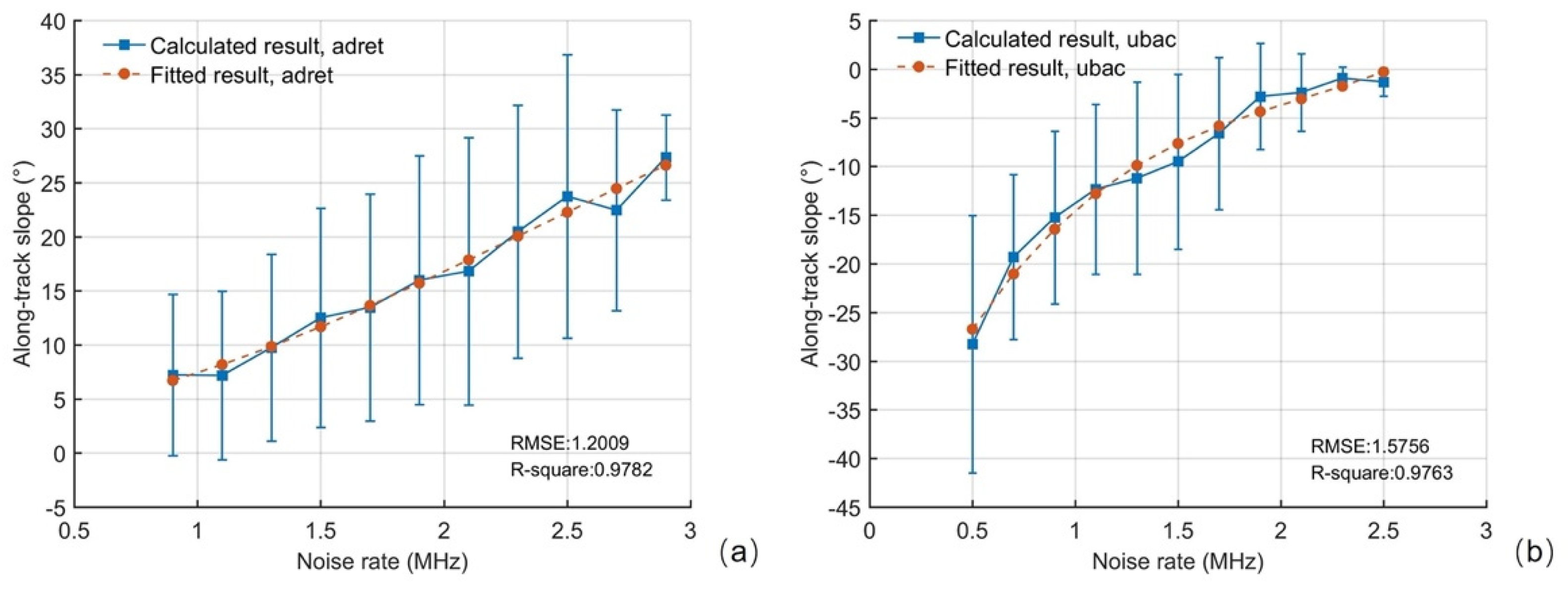
- Noise–slope relationship fitting
- (3)
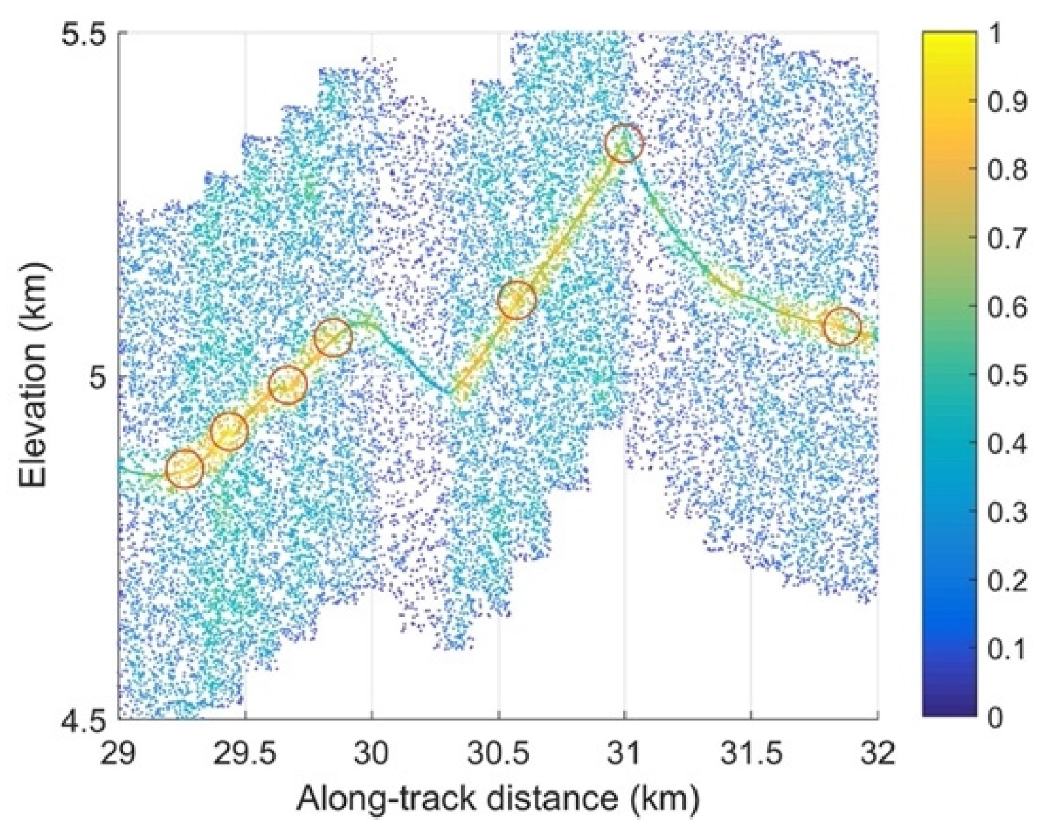
- Calculating parameters of the searching area and threshold in each cluster
- (4)
- Searching signal photons using the DBSCAN from weak beam data
- (5)
- Running a 3σ confidence filter to remove outliers
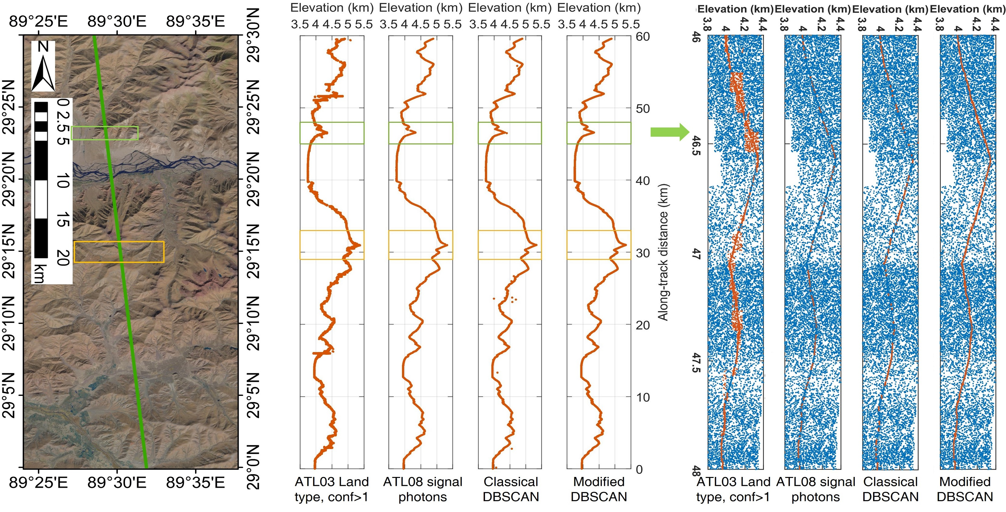
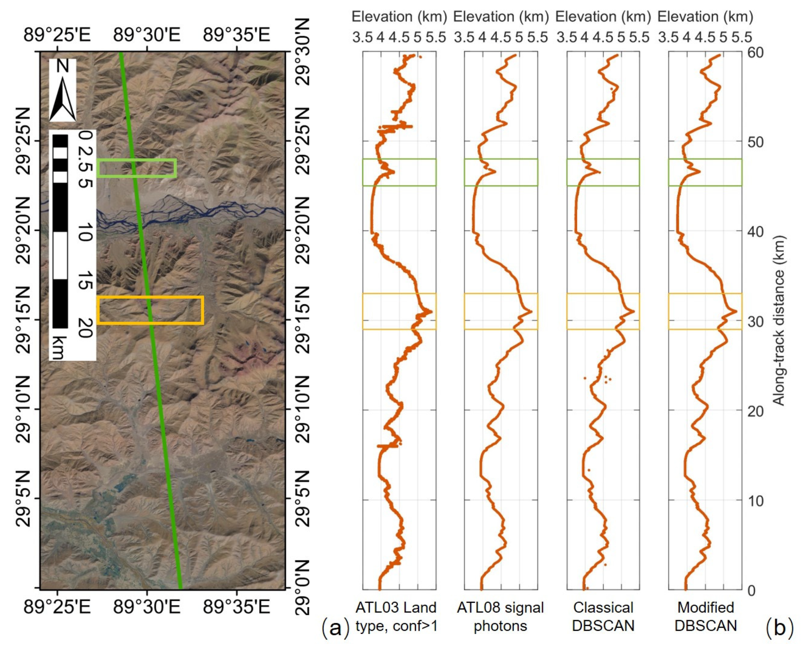
3. Results
4. Discussion
4.1. Precondition of Using the Algorithm
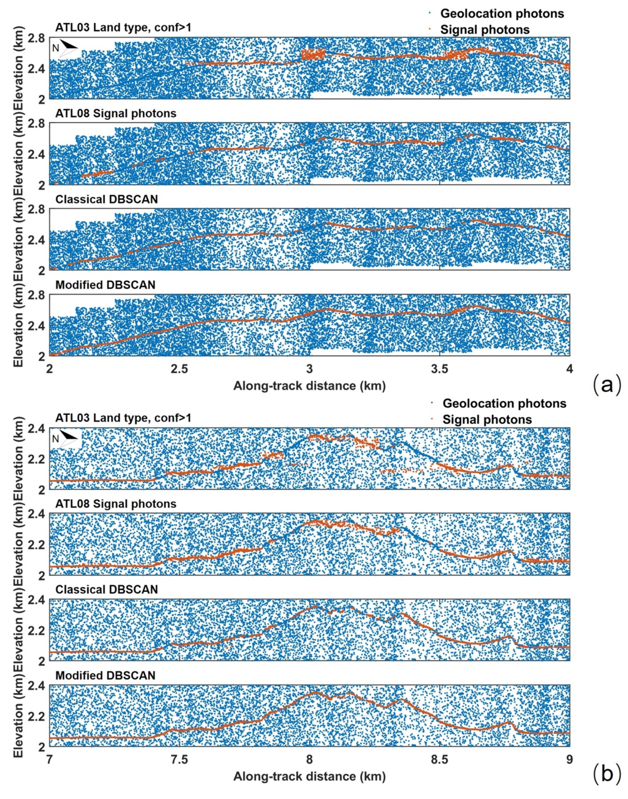
4.2. Why the Classical DBSCAN Failed
4.3. Potential Implications of the Algorithm
5. Conclusions
Supplementary Materials
Author Contributions
Funding
Institutional Review Board Statement
Informed Consent Statement
Data Availability Statement
Acknowledgments
Conflicts of Interest
Appendix A


References
- Brenner, A.C.; DiMarzio, J.P.; Zwally, H.J. Precision and accuracy of satellite radar and laser altimeter data over the continental ice sheets. IEEE Trans. Geosci. Remote Sens. 2007, 45, 321–331. [Google Scholar] [CrossRef]
- Price, D.; Rack, W.; Haas, C.; Langhorne, P.J.; Marsh, O. Sea ice freeboard in McMurdo Sound, Antarctica, derived by surface-validated ICESat laser altimeter data. J. Geophys. Res. Ocean. 2013, 118, 3634–3650. [Google Scholar] [CrossRef]
- Neuenschwander, A.L.; Urban, T.J.; Gutierrez, R.; Schutz, B.E. Characterization of ICESat/GLAS waveforms over terrestrial ecosystems: Implications for vegetation mapping. J. Geophys. Res. 2008, 113, G02S03. [Google Scholar] [CrossRef] [Green Version]
- Hilbert, C.; Schmullius, C. Influence of surface topography on ICESat/GLAS forest height estimation and waveform shape. Remote Sens. 2012, 4, 2210–2235. [Google Scholar] [CrossRef] [Green Version]
- Hajj, M.E.; Baghdadi, N.; Fayad, I.; Vieilledent, G.; Bailly, J.-S.; Minh, D.H.T. Interest of integrating spaceborne LiDAR data to improve the estimation of biomass in high biomass forested areas. Remote Sens. 2017, 9, 213. [Google Scholar] [CrossRef] [Green Version]
- Urban, T.J.; Schutz, B.E. ICESat sea level comparisons. Geophys. Res. Lett. 2005, 32, L23S10. [Google Scholar] [CrossRef] [Green Version]
- Schutz, B.E.; Zwally, H.J.; Shuman, C.A.; Hancock, D.; DiMarzio, J.P. Overview of the ICESat Mission. Geophys. Res. Lett. 2005, 32, L21S01. [Google Scholar] [CrossRef] [Green Version]
- Abshire, J.B.; Sun, X.; Riris, H.; Sirota, J.M.; McGarry, J.F.; Palm, S.; Yi, D.; Liiva, P. Geoscience Laser Altimeter System (GLAS) on the ICESat mission: On-orbit measurement performance. Geophys. Res. Lett. 2005, 32, L21S02. [Google Scholar] [CrossRef] [Green Version]
- Neuenschwander, A.L.; Magruder, L.A. Canopy and terrain height retrievals with ICESat-2: A first look. Remote Sens. 2019, 11, 1721. [Google Scholar] [CrossRef] [Green Version]
- Martino, A.J.; Neumann, T.A.; Kurtz, N.T.; McLennan, D. ICESat-2 mission overview and early performance. In Sensors, Systems, and Next-Generation Satellites XXIII; Neeck, S.P., Kimura, T., Martimort, P., Eds.; SPIE: Bellingham, WA, USA, 2019; p. 11. [Google Scholar]
- Markus, T.; Neumann, T.; Martino, A.; Abdalati, W.; Brunt, K.; Csatho, B.; Farrell, S.; Fricker, H.; Gardner, A.; Harding, D.; et al. The Ice, Cloud, and land Elevation Satellite-2 (ICESat-2): Science requirements, concept, and implementation. Remote Sens. Environ. 2017, 190, 260–273. [Google Scholar] [CrossRef]
- Tang, H.; Swatantran, A.; Barrett, T.; DeCola, P.; Dubayah, R. Voxel-based spatial filtering method for canopy height retrieval from airborne single-photon lidar. Remote Sens. 2016, 8, 771. [Google Scholar] [CrossRef] [Green Version]
- Wang, X.; Glennie, C.; Pan, Z. An adaptive ellipsoid searching filter for airborne single-photon lidar. IEEE Geosci. Remote Sens. Lett. 2017, 14, 1258–1262. [Google Scholar] [CrossRef]
- Li, Q.; Degnan, J.J.; Barrett, T.; Shan, J. First evaluation on single photon-sensitive lidar data. Photogramm. Eng. Remote Sens 2016, 82, 455–463. [Google Scholar] [CrossRef]
- Hernandez-Marin, S.; Wallace, A.M.; Gibson, G.J. Bayesian analysis of lidar signals with multiple returns. IEEE Trans. Pattern Anal. Mach. Intell. 2007, 29, 2170–2180. [Google Scholar] [CrossRef] [PubMed] [Green Version]
- Rapp, J.; Goyal, V.K. A Few photons among many: Unmixing signal and noise for photon-efficient active imaging. IEEE Trans. Comput. Imag. 2017, 3, 445–459. [Google Scholar] [CrossRef]
- Magruder, L.A.; Wharton, M.E.; Stout, K.D.; Neuenschwander, A.L. Noise filtering techniques for photon-counting Ladar data. In SPIE Defense, Security, and Sensing. International Society for Optics and Photonics; SPIE: Bellingham, WA, USA, 2012. [Google Scholar]
- Kwok, R.; Markus, T.; Morison, J.S.; Palm, P.; Neumann, T.A.; Brunt, K.M.; Cook, W.B.; Hancock, D.W.; Cunningham, G.F. Profiling sea ice with a Multiple Altimeter Beam Experimental Lidar (MABEL). J. Atmos. Ocean. Technol. 2014, 31, 1151–1168. [Google Scholar] [CrossRef] [Green Version]
- Herzfeld, U.C.; McDonald, B.W.; Wallin, B.F.; Neumann, T.A.; Markus, T.; Brenner, A.; Field, C. Algorithm for detection of ground and canopy cover in micropulse photon-counting lidar altimeter data in preparation for the ICESat-2 mission. IEEE Trans. Geosci. Remote Sens. 2014, 52, 2109–2125. [Google Scholar] [CrossRef]
- Moussavi, M.S.; Abdalati, W.; Scambos, T.; Neuenschwander, A. Applicability of an automatic surface detection approach to micro-pulse photon-counting lidar altimetry data: Implications for canopy height retrieval from future ICESat-2 data. Int. J. Remote Sens. 2014, 35, 5263–5279. [Google Scholar] [CrossRef]
- Gwenzi, D.; Lefsky, M.A.; Suchdeo, V.P.; Harding, D.J. Prospects of the ICESat-2 laser altimetry mission for Savanna ecosystem structural studies based on airborne simulation data. ISPRS J. Photogramm. Remote Sens. 2016, 118, 68–82. [Google Scholar] [CrossRef]
- Herzfeld, U.C.; Trantow, T.M.; Harding, D.; Dabney, P.W. Surface-height determination of crevassed glaciers—Mathematical principles of an autoadaptive density-dimension algorithm and validation using ICESat-2 simulator (SIMPL) data. IEEE Trans. Geosci. Remote Sens. 2017, 55, 1874–1896. [Google Scholar] [CrossRef]
- Popescu, S.C.; Zhou, T.; Nelson, R.; Neuenschwander, A.; Sheridan, R.; Narine, L.; Walsh, K.M. Photon counting LiDAR: An adaptive ground and canopy height retrieval algorithm for ICESat-2 data. Remote Sens. Environ. 2018, 208, 154–170. [Google Scholar] [CrossRef]
- Neuenschwander, A.; Pitt, K. The ATL08 land and vegetation product for the ICESat-2 Mission. Remote Sens. Environ. 2019, 221, 247–259. [Google Scholar] [CrossRef]
- Smith, B.; Fricker, H.A.; Holschuh, N.; Gardner, A.S.; Adusumilli, S.; Brunt, K.M.; Csatho, B.; Harbeck, K.; Huth, A.; Neumann, T.; et al. Land ice height-retrieval algorithm for NASA’s ICESat-2 photon-counting laser altimeter. Remote Sens. Environ. 2019, 233, 111352–111368. [Google Scholar] [CrossRef] [Green Version]
- Liu, M.; Popescu, S.; Malambo, L. Feasibility of burned area mapping based on ICESAT−2 photon counting data. Remote Sens. 2019, 12, 24. [Google Scholar] [CrossRef] [Green Version]
- Neuenschwander, A.L.; Pitts, K.L.; Jelley, B.P.; Robbins, J.; Klotz, B.; Popescu, S.C.; Nelson, R.F.; Harding, D.; Pederson, D.; Sheridan, R. ICE, CLOUD, and Land Elevation Satellite-2 (ICESat-2) Algorithm Theoretical Basis Document (ATBD) for Land-Vegetation Along-Track Products(ATL08); Land/Vegetation SDT Team Members and ICESat-2 Project Science Office: Greenbelt, MD, USA, 2020. [Google Scholar]
- Morison, J.; Hancock, D.; Dickinson, J.; Robbins, T.; Roberts, L.; Kwok, R.; Palm, S.; Jasinski, M.; Plant, B.; Urban, T. ICE, CLOUD, and Land Elevation Satellite-2 (ICESat-2) Project Algorithm Theoretical Basis Document (ATBD) for Ocean Surface Height (ATL12); Goddard Space Flight Center: Greenbelt, MD, USA, 2020. [Google Scholar]
- Jasinski, M.; Stoll, J.; Hancock, D.; Robbins, J.; Nattala, J.; Morison, J.; Jones, B.; Ondrusek, M.; Pavelsky, T.; Parrish, C.; et al. ICE, CLOUD, and Land Elevation Satellite-2 (ICESat-2) Project Algorithm Theoretical Basis Document (ATBD) for Inland Water Data Products (ATL13); Goddard Space Flight Center: Greenbelt, MD, USA, 2020. [Google Scholar]
- Malambo, L.; Popescu, S.C. PhotonLabeler: An inter-disciplinary platform for bisual interpretation and labeling of ICESat-2 geolocated photon data. Remote Sens. 2020, 12, 3168. [Google Scholar] [CrossRef]
- Wang, X.; Pan, Z.; Glennie, C. A novel noise filtering model for photon-counting laser altimeter data. IEEE Geosci. Remote Sens. Lett. 2016, 13, 947–951. [Google Scholar] [CrossRef]
- Zhang, J.; Kerekes, J.; Csatho, B.; Schenk, T.; Wheelwright, R. A clustering approach for detection of ground in micropulse photon-counting LiDAR altimeter data. In Proceedings of the IEEE Geoscience and Remote Sensing Symposium, Quebec City, QC, Canada, 13–18 July 2014; pp. 177–180. [Google Scholar]
- Ester, M.; Kriegel, H.-P.; Sander, J.; Xu, X. A density-based algorithm for discovering clusters in large spatial databases with noise. In Proceedings of the Second International Conference on Knowledge Discovery and Data Mining (KDD-96), Portland, OR, USA, 2–4 August 1996; pp. 226–231. [Google Scholar]
- Ma, Y.; Zhang, W.; Sun, J.; Li, G.; Wang, X.; Li, S.; Xu, N. Photon-counting lidar: An adaptive signal detection method for different land cover types in coastal areas. Remote Sens. 2019, 11, 471. [Google Scholar] [CrossRef] [Green Version]
- Nie, S.; Wang, C.; Xi, X.; Luo, S.; Li, G.; Tian, J.; Wang, H. Estimating the vegetation canopy height using micro-pulse photon-counting LiDAR data. Opt. Express 2018, 26, A520–A540. [Google Scholar] [CrossRef]
- Zhu, X.; Nie, S.; Wang, C.; Xi, X.; Hu, Z. A ground elevation and vegetation height retrieval algorithm using micro-pulse photon-counting Lidar data. Remote Sens. 2018, 10, 1962. [Google Scholar] [CrossRef] [Green Version]
- Zhu, X.; Nie, S.; Wang, C.; Xi, X.; Wang, J.; Li, D.; Zhou, H. A noise removal algorithm based on OPTICS for photon-counting LiDAR data. IEEE Geosci. Remote Sens. Lett. 2020. [Google Scholar] [CrossRef]
- Huang, J.; Xing, Y.; You, H.; Qin, L.; Tian, J.; Ma, J. Particle swarm optimization-based noise filtering algorithm for photon cloud data in forest area. Remote Sens. 2019, 11, 980. [Google Scholar] [CrossRef] [Green Version]
- Brunt, K.M.; Neumann, T.A.; Amundson, J.M.; Kavanaugh, J.L.; Moussavi, M.S.; Walsh, K.M.; Cook, W.B.; Markus, T. MABEL photon-counting laser altimetry data for ICESat-2 simulations and development. Cryosphere 2016, 10, 1707–1719. [Google Scholar] [CrossRef] [Green Version]
- Neumann, T.A.; Martino, A.J.; Markus, T.; Bae, S.; Bock, M.R.; Brenner, A.C.; Brunt, K.M.; Cavanaugh, J.; Fernandes, S.T.; Hancock, D.W.; et al. The Ice, Cloud, and Land Elevation Satellite-2 mission: A global geolocated photon product derived from the Advanced Topographic Laser Altimeter System. Remote Sens. Environ. 2019, 233, 111325–111341. [Google Scholar] [CrossRef] [PubMed]
- Yang, G.; Martino, A.J.; Lu, W.; Cavanaugh, J.F.; Bock, M.R.; Krainak, M.A. IceSat-2 ATLAS photon-counting receiver: Initial on-orbit performance. In Advanced Photon Counting Techniques XIII; Itzler, M.A., McIntosh, K.A., Bienfang, J.C., Eds.; SPIE: Bellingham, WA, USA, 2019; p. 10. [Google Scholar]
- Neumann, T.A.; Brenner, A.; Hancock, D.; Robbins, J.; Saba, J.; Harbeck, K.; Gibbons, A.; Lee, J.; Luthcke, S.B.; Rebold, T.; et al. ATLAS/ICESat-2 L2A Global Geolocated Photon Data, Version 3; NASA National Snow and Ice Data Center Distributed Active Archive Center: Boulder, CO, USA, 2020. [CrossRef]
- Neumann, T.; Brenner, A.; Hancock, D.; Robbins, J.; Saba, J.; Harbeck, K.; Gibbons, A. ICE, CLOUD, and Land Elevation Satellite-2 (ICESat-2) Project Algorithm Theoretical Basis Document (ATBD) for Global Geolocated Photons ATL03; Goddard Space Flight Center: Greenbelt, MD, USA, 2019. [Google Scholar]
- McGill, M.; Markus, T.; Scott, V.S.; Neumann, T. The Multiple Altimeter Beam Experimental Lidar (MABEL): An Airborne Simulator for the ICESat-2 Mission. J. Atmos. Ocean. Technol. 2013, 30, 345–352. [Google Scholar] [CrossRef]
- Neuenschwander, A.L.; Pitts, K.L.; Jelley, B.P.; Robbins, J.; Klotz, B.; Popescu, S.C.; Nelson, R.F.; Harding, D.; Pederson, D.; Sheridan, R. ATLAS/ICESat-2 L3A Land and Vegetation Height, Version 3; NASA National Snow and Ice Data Center Distributed Active Archive Center: Boulder, CO, USA, 2020. [CrossRef]
- Degnan, J.J. Photon-counting multikilohertz microlaser altimeters for airborne and spaceborne topographic measurements. J. Geodyn. 2002, 34, 503–549. [Google Scholar] [CrossRef] [Green Version]
- Li, S.; Zhang, Z.; Ma, Y.; Zeng, H.; Zhao, P.; Zhang, W. Ranging performance models based on negative-binomial (NB) distribution for photon-counting lidars. Opt. Express 2019, 27, A861–A877. [Google Scholar] [CrossRef]
- Gardner, C.S. Target signatures for laser altimeters: An analysis. Appl. Opt. 1982, 21, 448–453. [Google Scholar] [CrossRef]
- Greeley, A.P.; Neumann, T.A.; Kurtz, N.T.; Markus, T.; Martino, A.J. Characterizing the system impulse response function from photon-counting LiDAR data. IEEE Trans. Geosci. Remote Sens. 2019, 57, 6542–6551. [Google Scholar] [CrossRef]
- Gatt, P.; Johnson, S.; Nichols, T. Geiger-mode avalanche photodiode ladar receiver performance characteristics and detection statistics. Appl. Opt. 2009, 48, 3261–3276. [Google Scholar] [CrossRef]
- Ma, Y.; Li, S.; Zhang, W.; Zhang, Z.; Liu, R.; Wang, X.H. Theoretical ranging performance model and range walk error correction for photon-counting lidars with multiple detectors. Opt. Express 2018, 26, 15924–15934. [Google Scholar] [CrossRef]
- Zhang, Z.; Xu, N.; Ma, Y.; Liu, X.; Zhang, W.; Li, S. Land and snow-covered area classification method based on the background noise for satellite photon-counting laser altimeters. Opt. Express 2020, 28, 16030–16044. [Google Scholar] [CrossRef] [PubMed]
- Heris, M.K. DBSCAN Clustering in MATLAB; Yarpiz, 2015; Available online: https://yarpiz.com/255/ypml110-dbscan-clustering (accessed on 7 September 2015).
- Hripcsak, G. Agreement, the F-measure, and reliability in information retrieval. J. Am. Med. Inform. Assoc. 2005, 12, 296–298. [Google Scholar] [CrossRef] [PubMed]
- Neuenschwander, A.; Guenther, E.; White, J.C.; Duncanson, L.; Montesano, P. Validation of ICESat-2 terrain and canopy heights in boreal forests. Remote Sens. Environ. 2020, 251, 112110. [Google Scholar] [CrossRef]
- Tian, X.; Shan, J. Comprehensive evaluation of the ICESat-2 ATL08 terrain product. IEEE Trans. Geosci. Remote Sens. 2021. [Google Scholar] [CrossRef]
- Brunt, K.M.; Smith, B.; Suterley, T.; Kurtz, N.; Neumann, T. Comparisons of satellite and airborne altimetry with ground-based data from the interior of the Antarctic ice sheet. Geophys. Res. Lett. 2020, 48, e2020GL090572. [Google Scholar]
- Farrell, S.L.; Duncan, K.; Buckley, E.M.; Richter-Menge, J.; Li, R. Mapping Sea Ice Surface Topography in High Fidelity with ICESat-2. Geophys. Res. Lett. 2020, 47, e2020GL090708. [Google Scholar] [CrossRef]
- Li, G.; Tang, X.; Gao, X.; Wang, H.; Wang, Y. ZY-3 Block adjustment supported by GLAS laser altimetry data. Photogramm. Rec. 2016, 31, 88–107. [Google Scholar] [CrossRef]


| Site Name | Geographical Location | ICESat-2 Data | Sentinel-2 Image | ||
|---|---|---|---|---|---|
| Acquisition Date and Season | Local Time | Acquisition Date | Environment | ||
| Site 1: in the Tibetan Plateau I | 29°0′–29°30′ N, 89°25′–89°35′ E | 7 December 2018 in early winter | 12:56 a.m. | 6 December 2018 | Elevation above 3700 m, covered by bare-land, sparse grasslands, and rivers (in the valley) |
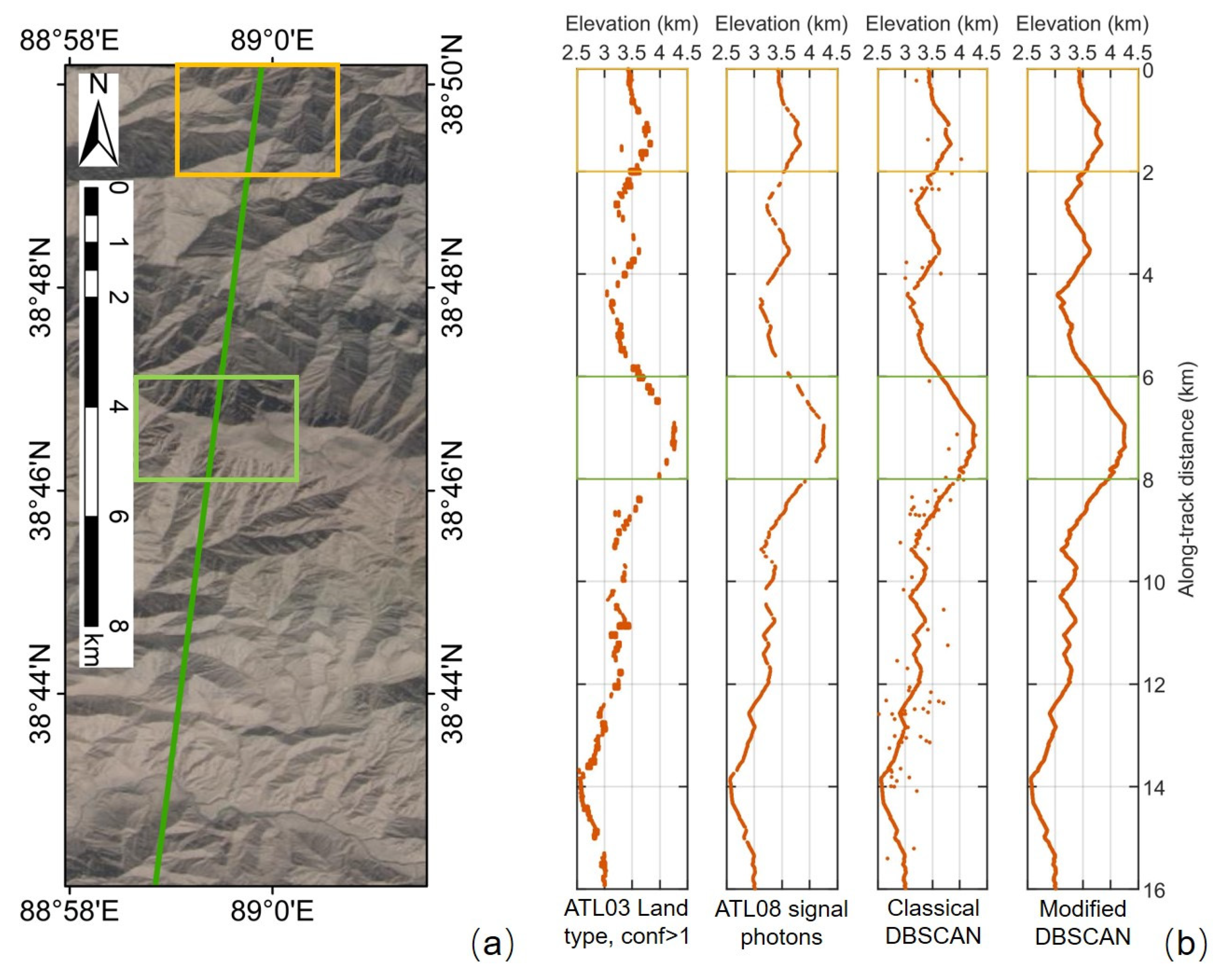
| Site 2: in the Altun Mountains II | 38°41′–38°51′ N, 88°58′–89°01′ E | 29 September 2019 in autumn | 10:56 a.m. | 3 October 2019 | Elevation above 2500 m, covered by bare-land and very sparse grasslands |
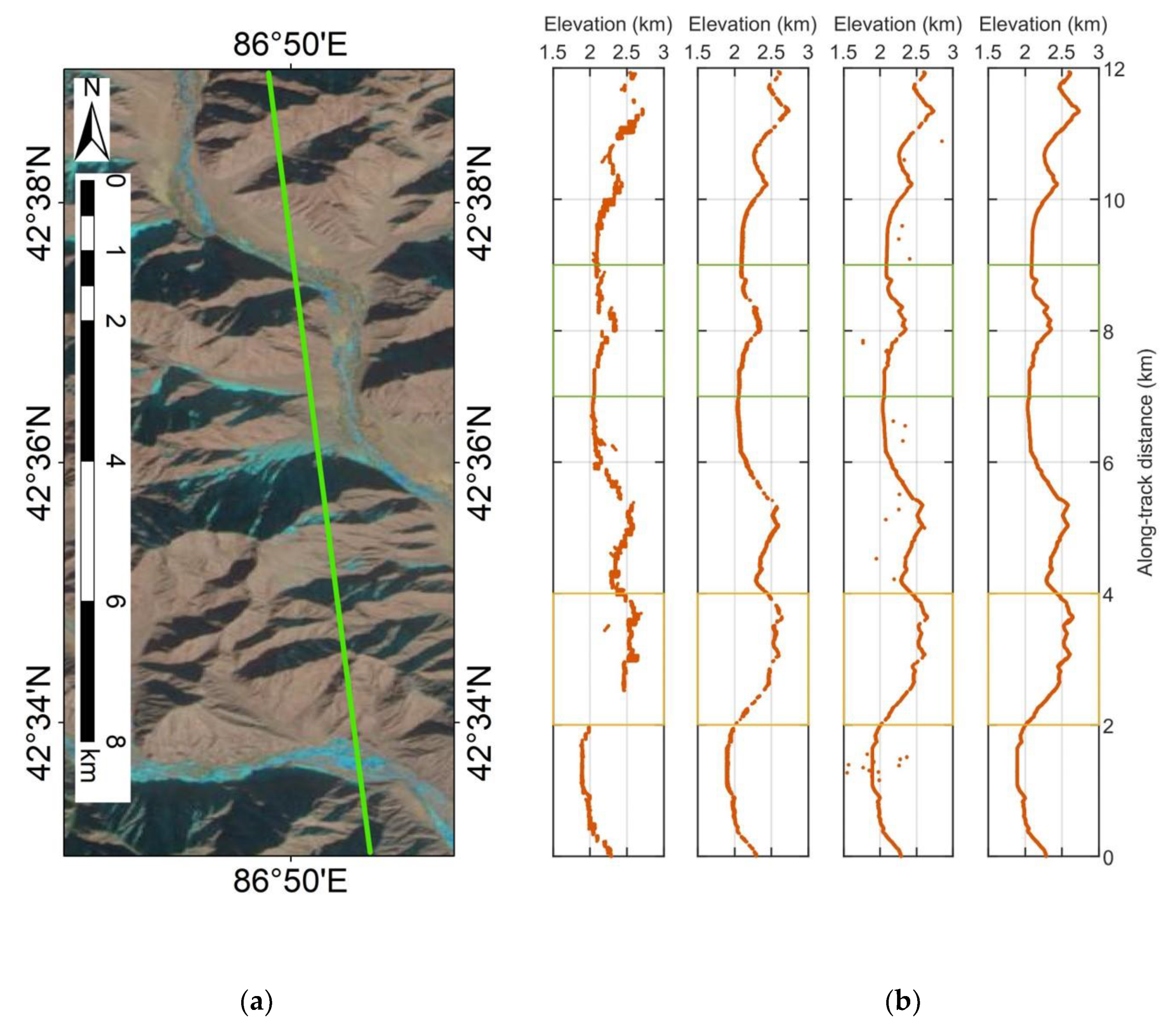
| Site 3: in the Tian Shan Mountains III | 42°32′–42°40′ N, 86°49′–86°51′ E | 13 February 2019 in late winter | 9:35 a.m. | 13 February 2019 | Elevation above 1800 m, covered by bare-land and sparse snow |
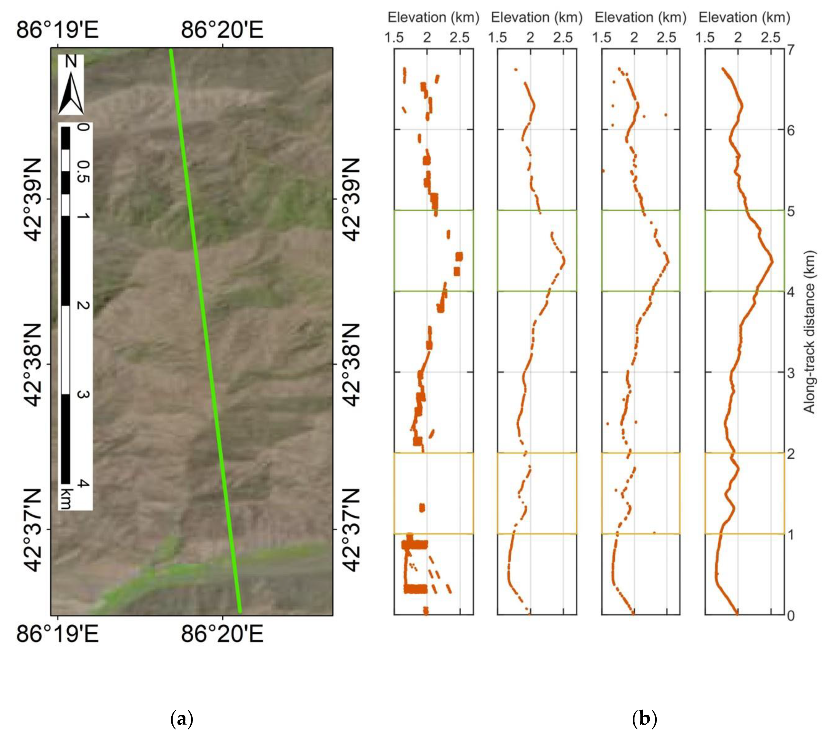
| Site 4: in the Tian Shan Mountains IV | 42°36′–42°40′ N, 86°19′–86°21′ E | 12 June 2020 in summer | 10:39 a.m. | 22 June 2020 | Elevation above 1700 m, covered by bare-land and grasslands |
| Parameter | Value | Parameter | Value |
|---|---|---|---|
| Filter bandpass, Δλ | 38 pm | Wavelength, λ | 532 nm |
| Effective aperture area, Ar | 0.41 m2 | Flight height, z | 500 km |
| Transmitting telescope efficiency, ηt | 40% | Receiving FOV, θr | 85 μrad |
| Receiving telescope efficiency, ηr | 50.4% | Laser nadir angle, θp | 0° or 0.38° |
| Detector quantum efficiency, ηQE | 15% | Detector dead-time, Td | 3.2 ns |
| Half of the laser beam divergence, θT | 8.75 μrad at e−1/2 | Transmitted pulse width, σf | 1.5 ns (FWHM) |
| Laser energy of strong beam, E0 | 95.7 μJ I | Laser energy of weak beam, E0 | 22.2 μJ II |
| Location/Time | Ground Truth | ATL03 | ATL08 | Classical DBSCAN | Modified DBSCAN | ||||
|---|---|---|---|---|---|---|---|---|---|
| Signal Photon | Noise Photon | Signal Photon | Noise Photon | Signal Photon | Noise Photon | Signal Photon | Noise Photon | ||
| Area 1 In the Tibetan Plateau In early winter | Signal photon | 56,914 (TP) | 3074 (FN) | 29,297 | 30,691 | 45,070 | 14,918 | 57,386 | 2602 |
| Noise photon | 22,274 (FP) | 531,067 (TN) | 204 | 553,137 | 595 | 552,746 | 3318 | 550,023 | |
| Precision, Ppre | 71.87% | 99.31% | 98.70% | 94.53% | |||||
| Recall, Prec | 94.88% | 48.84% | 75.13% | 95.66% | |||||
| F-score | 0.8178 | 0.6548 | 0.8532 | 0.9510 | |||||
| Area 2 In the Altun Mountains In autumn | Signal photon | 12,360 | 11,814 | 4308 | 19,866 | 11,219 | 12,955 | 22,509 | 1665 |
| Noise photon | 6148 | 330,307 | 38 | 336,417 | 505 | 335,950 | 270 | 336,185 | |
| Precision, Ppre | 66.78% | 99.13% | 95.69% | 98.81% | |||||
| Recall, Prec | 51.13% | 17.82% | 46.41% | 93.11% | |||||
| F-score | 0.5792 | 0.3021 | 0.6250 | 0.9588 | |||||
| Area 3 In the Tian Shan Mountains In late winter | Signal photon | 11,832 | 4365 | 11,765 | 4432 | 11,958 | 4239 | 14,666 | 1531 |
| Noise photon | 2768 | 108,943 | 1333 | 110,378 | 2972 | 110,378 | 318 | 111,393 | |
| Precision, Ppre | 81.04% | 89.82% | 80.09% | 97.88% | |||||
| Recall, Prec | 73.05% | 72.64% | 73.83% | 90.55% | |||||
| F-score | 0.7684 | 0.8032 | 0.7383 | 0.9407 | |||||
| Area 4 In the Tian Shan Mountains In summer | Signal photon | 2638 | 2536 | 881 | 4293 | 2702 | 2472 | 4038 | 1136 |
| Noise photon | 4884 | 147,877 | 119 | 152,642 | 4968 | 147,793 | 843 | 151,918 | |
| Precision, Ppre | 35.07% | 88.10% | 35.23% | 82.73% | |||||
| Recall, Prec | 50.99% | 17.03% | 52.22% | 78.04% | |||||
| F-score | 0.4156 | 0.2854 | 0.4207 | 0.8032 | |||||
Publisher’s Note: MDPI stays neutral with regard to jurisdictional claims in published maps and institutional affiliations. |
© 2021 by the authors. Licensee MDPI, Basel, Switzerland. This article is an open access article distributed under the terms and conditions of the Creative Commons Attribution (CC BY) license (http://creativecommons.org/licenses/by/4.0/).
Share and Cite
Zhang, Z.; Liu, X.; Ma, Y.; Xu, N.; Zhang, W.; Li, S. Signal Photon Extraction Method for Weak Beam Data of ICESat-2 Using Information Provided by Strong Beam Data in Mountainous Areas. Remote Sens. 2021, 13, 863. https://doi.org/10.3390/rs13050863
Zhang Z, Liu X, Ma Y, Xu N, Zhang W, Li S. Signal Photon Extraction Method for Weak Beam Data of ICESat-2 Using Information Provided by Strong Beam Data in Mountainous Areas. Remote Sensing. 2021; 13(5):863. https://doi.org/10.3390/rs13050863
Chicago/Turabian StyleZhang, Zhiyu, Xinyuan Liu, Yue Ma, Nan Xu, Wenhao Zhang, and Song Li. 2021. "Signal Photon Extraction Method for Weak Beam Data of ICESat-2 Using Information Provided by Strong Beam Data in Mountainous Areas" Remote Sensing 13, no. 5: 863. https://doi.org/10.3390/rs13050863